
Submitted:
04 September 2025
Posted:
05 September 2025
You are already at the latest version
Abstract
Intermediate-mass black holes (IMBHs; $\Mbh \approx 10^{3-5}\Msun$) play a critical role in understanding the formation of supermassive black holes in the early universe. In this study, we expand on Nguyen et al. simulated measurements of IMBH masses using stellar kinematics, which will be observed with the High Angular Resolution Monolithic Optical and Near-infrared Integral (HARMONI) field spectrograph on the Extremely Large Telescope (ELT) up to the distance of 20 Mpc. Our sample focuses on both the Virgo Cluster in the northern sky and the Fornax Cluster in the southern sky. We begin by identifying dwarf galaxies hosting nuclear star clusters, which are thought to be nurseries for IMBHs in the local universe. As a case study, we conduct simulations for FCC 119, the second faintest dwarf galaxies in the Fornax Cluster at 20 Mpc, which is also fainter than most of Virgo Cluster members. We use the galaxy’s surface brightness profile from Hubble Space Telescope (HST) imaging, combined with an assumed synthetic spectrum, to create mock observations with the {\tt HSIM} simulator and Jeans Anisotropic Models (JAM). These mock HARMONI datacubes are analyzed as if they were real observations, employing JAM within a Bayesian framework to infer IMBH masses and their associated uncertainties. We find that ELT/HARMONI can detect the stellar kinematic signature of an IMBH and accurately measure its mass for $\Mbh \gtrsim 10^5~\Msun$ out to distances of $\sim$20 Mpc.
Keywords:
galaxies
; individual
; FCC 119 – galaxies
; supermassive black holes – galaxies
; nuclei – galaxies
; kinematics
; dynamics – galaxies
; evolution – galaxies
; formation
1. Introduction
Intermediate-mass black holes (IMBHs; ) in dwarf galaxies () represent a crucial but largely missing component of the black hole (BH) mass spectrum [60,90]. Studying the correlations between IMBH mass and the macroscopic properties of their host galaxies—such as central stellar velocity dispersion () [45,51] or bulge stellar mass () [75]—provides valuable insights when compared to their supermassive black hole (SMBH; ) counterparts in more massive galaxies (). Additionally, determining the occupation fraction—the proportion of dwarf galaxies hosting IMBHs—can constrain potential formation pathways of these black holes in the early universe [61]. Despite extensive searches [61], the presence of IMBHs remains elusive, and their origins continue to be an open question in astrophysics [69,94].
Despite the fact that dynamical methods using stellar or gas motions in the centers of nearby dwarf galaxies are among the most precise techniques for searching for strong evidence of IMBHs [1,34,36,96,97,99,100,101,102,103,104,105,131,132,135,148], they remain observationally challenging due to the insufficient spatial resolution of current facilities [99,122] to resolve the black hole’s sphere of influence (SOI), defined as , where G is the gravitational constant. For example, for an IMBH with M⊙ and km s−1 at the distance of the Local Group ( Mpc), the corresponding [e.g., see Eq. 1 of [98]], which is smaller than the diffraction limits of current 8–10 meter class ground-based telescopes equipped with adaptive optics (AO), which achieve point-spread functions (PSFs) with typical full widths at half maximum (FWHM) in the range of –. This limitation raises the question of whether the current lack of strong observational evidence for IMBHs reflects their true absence, or simply the restrictions imposed by existing instrumentation.
The next generation of giant ground-based telescopes may provide a solution to this problem. In particular, the Extremely Large Telescope (ELT) is poised to overcome current resolution challenges with its 39 meter primary mirror, equipped with the Multi-AO Imaging Camera for Deep Observations (MICADO; ) imager [32,33] and the High Angular Resolution Monolithic Optical and Near-infrared Integral (HARMONI; ) field spectrograph, which also offers a high-spectral resolution () [136,137]. However, to locate potential IMBHs, we must first identify suitable targets. According to [106], bright nuclear star clusters (NSCs) within 10 Mpc are promising hosts of IMBHs. These IMBHs can be dynamically detected if their masses are at least ∼0.5% of their NSC mass (), although the effects of dynamical mass segregation must be carefully considered before drawing strong conclusions.
In this study, we extend the distance limit of the HARMONI IMBH survey [106] to include the Virgo ( Mpc) and Fornax ( Mpc) clusters by simulating measurements for FCC 119, the second faintest nucleated member of the Fornax Cluster and significantly fainter than nearly all members of the Virgo Cluster. These measurements are derived from high-spatial-resolution integral-field unit (IFU) stellar kinematics extracted from mock HARMONI data, generated using the HARMONI Simulator (HSIM1) [155]. We also investigate the observational limits in terms of the minimum NSC central surface brightness (SB), IMBH mass, and on source exposure time that HARMONI can effectively detect.
We describe the criteria used to finalize the extended HARMONI IMBH sample and its properties, as well as the characteristics of the Virgo and Fornax Clusters, which contain a significant portion of our sample, in Section 2. In Section 3, we present the stellar mass model of FCC 119. Section 4 provides a detailed description of our HARMONI IFS simulations. Finally, we discuss the results in Section 5 and summarize our findings in Section 6.
We adopt a flat Universe with a Hubble constant of km s−1 Mpc−1, a matter density of , and a dark energy density of . All photometric measurements are reported in the AB magnitude system [108] and corrected for foreground extinction [119] using a interstellar extinction law [24]. Furthermore, all kinematic maps are aligned such that the galaxy’s major and minor axes correspond to the horizontal and vertical directions, respectively.
2. Sample Selection
2.1. Sample Selection
We compiled a list of known nucleated dwarf galaxies from previous NSC surveys, including both photometry and spectroscopy [5,13,22,42,43,53,54,56,58,59,65,67,95,112,115,126], to create a parent sample for selecting the best candidates likely to host IMBHs beyond the current HARMONI IMBH sample within 10 Mpc [106], extending the survey out to 20 Mpc. The selection criteria are listed in the upper part of Table 1.
2.2. Sample Properties
We present in Figure 1 our selected targets on the distance–magnitude plane and compare them with previous galaxy surveys, including MMBH [98], MASSIVE [84], ATLAS3D [22], and the HARMONI IMBH survey [106]. We calculated the absolute magnitude in the -band using the relation , calibrated from a sample of 260 elliptical galaxies within 48 Mpc in the ATLAS3D project [22]. Here, magnitudes are sourced from the NED-D2 and HyperLeda3 databases, while represents the Galactic extinction in the Landolt V-band [119], adopting the [25] reddening relation with .
We summarized in Table 2 our expanded HARMONI IMBH sample, spanning a distance range of Mpc and an absolute -band magnitude range of . It overlaps with the ATLAS3D survey by 2.2 mag ( mag) and focuses more on lower-mass galaxies. Additionally, our sample is distinct from the 10 Mpc HARMONI IMBH sample [106], although both samples cover nearly the same stellar mass range of to . Our selected galaxies also exhibit central stellar velocity dispersions ranging from 16 to 75 km s−1.
This expanded HARMONI IMBH sample comprises 85 galaxies, including 29 and 20 members of the Virgo (prefix VCC) and Fornax (prefix FCC) Clusters, respectively, along with 36 isolated dwarf galaxies or members of other groups, as detailed in Table 4. It spans a diverse range of galaxy morphologies, consisting of 27% ellipticals, 29% lenticulars, 39% spirals, and 5% irregulars. These galaxies host luminous NSCs with masses in the range and effective radii spanning pc, as shown in Figure 2 for the – and – relationships.

Table 3.
Full list and properties of our extended HARMONI IMBH sample hosting NSCs within the distant range of 10–20 Mpc
Table 3.
Full list and properties of our extended HARMONI IMBH sample hosting NSCs within the distant range of 10–20 Mpc
| No. | Object | RA | Decl. | D | Hubble | Ref. | |||||
| name | (h:m:s) | (d:m:s) | (Mpc) | type | () | (kpc) | () | (pc) | (km s−1) | ||
| (1) | (2) | (3) | (4) | (5) | (6) | (7) | (8) | (9) | (10) | (11) | (12) |
| 1 | ESO301-IG11 | 03:23:54.21 | −37:30:33.0 | 19.94 | 9.9 | 9.61 | 2.11 | 5.79 | 3.7 | 28.9 | [54] |
| 2 | IC1933 | 03:25:39.97 | −52:47:07.5 | 18.98 | 6.1 | 8.35 | 1.85 | 5.21 | 6.2 | 42.7 | [54] |
| 3 | MCG-1-03-85 | 01:05:04.88 | −06:12:44.6 | 11.38 | 7.0 | 9.66 | 4.04 | 6.40 | 2.9 | 42.0 | [5,54] |
| 4 | NGC0428 | 01:12:55.75 | +00:58:53.5 | 16.54 | 8.6 | 9.54 | 2.63 | 6.41 | 1.2 | 56.9 | [54] |
| 5 | NGC0864 | 02:15:27.64 | +06:00:09.4 | 19.41 | 5.1 | 10.10 | 0.21 | 7.86 | 2.7 | 26.9 | [54,65] |
| 6 | NGC1042 | 02:40:23.97 | −08:26:00.7 | 19.59 | 6.0 | 9.32 | 4.59 | 6.33 | 1.3 | 65.3 | [54] |
| 7 | NGC1073 | 02:43:40.52 | +01:22:34.0 | 13.80 | 5.3 | 9.69 | 0.16 | 6.53 | 0.5 | 24.8 | [54,65] |
| 8 | NGC1493 | 03:57:27.46 | −46:12:38.6 | 15.54 | 6.0 | 9.77 | 4.85 | 6.55 | 3.6 | 51.2 | [54] |
| 9 | NGC1518 | 04:06:49.82 | −21:10:23.5 | 13.50 | 8.2 | 9.10 | 0.83 | 5.35 | 3.4 | 36.6 | [54] |
| 10 | NGC1559 | 04:17:35.77 | −62:47:01.2 | 15.21 | 5.9 | 9.77 | 3.50 | 6.66 | 1.5 | 72.6 | [5,54,130] |
| 11 | NGC2835 | 09:17:52.91 | −22:21:16.8 | 10.86 | 5.0 | 9.70 | 2.80 | 6.61 | 3.4 | 70.7 | [5,54,130] |
| 12 | NGC3346 | 10:43:38.91 | +14:52:18.9 | 17.84 | 5.9 | 9.51 | 3.34 | 6.37 | 1.1 | 49.6 | [54] |
| 13 | NGC3423 | 10:51:14.33 | +05:50:24.1 | 11.27 | 6.0 | 9.45 | 0.12 | 6.29 | 2.2 | 54.6 | [54] |
| 14 | NGC3455 | 10:54:31.08 | +17:17:04.6 | 15.79 | 3.7 | 10.57 | 1.44 | 6.81 | 2.2 | 46.2 | [54] |
| 15 | NGC3666 | 11:24:26.07 | +11:20:32.0 | 19.32 | 5.2 | 9.94 | 0.10 | 7.81 | 9.6 | 60.6 | [54,65] |
| 16 | NGC4212 | 12:15:39.36 | +13:54:05.4 | 17.30 | 4.9 | 10.40 | 4.56 | 6.70 | 12.3 | 61.0 | [54,59] |
| 17 | NGC4487 | 12:31:04.46 | −08:03:14.1 | 19.59 | 6.0 | 10.38 | 3.50 | 6.93 | 1.1 | 51.0 | [54] |
| 18 | NGC4496A | 12:31:39.21 | +03:56:22.1 | 15.49 | 7.6 | 9.65 | 3.10 | 6.23 | 0.7 | 74.9 | [54,65,130] |
| 19 | NGC4504 | 12:32:17.41 | −07:33:48.9 | 14.51 | 6.0 | 10.54 | 2.10 | 6.85 | 3.9 | 53.0 | [54] |
| 20 | NGC4517 | 12:32:45.59 | +00:06:54.1 | 10.67 | 6.0 | 10.08 | 6.50 | 5.85 | 2.3 | 43.8 | [54,65] |
| 21 | NGC4592 | 12:39:18.74 | −00:31:55.0 | 15.21 | 8.0 | 10.28 | 1.84 | 5.80 | 1.1 | 42.6 | [54] |
| 22 | NGC4635 | 12:42:39.23 | +19:56:43.7 | 13.54 | 6.6 | 9.01 | 1.40 | 6.79 | 4.3 | 34.7 | [54] |
| 23 | NGC4771 | 12:53:21.26 | +01:16:09.5 | 16.07 | 6.2 | 10.32 | 2.73 | 6.63 | 1.9 | 64.4 | [54] |
| 24 | NGC4900 | 13:00:39.26 | +02:30:02.7 | 13.73 | 5.2 | 10.12 | 2.59 | 7.24 | 3.1 | 67.1 | [54] |
| 25 | NGC4904 | 13:00:58.64 | −00:01:39.4 | 16.94 | 5.8 | 9.92 | 2.06 | 6.23 | 2.5 | 62.5 | [54] |
| 26 | NGC5054 | 13:16:58.49 | −16:38:05.5 | 18.62 | 4.2 | 10.43 | 0.11 | 7.02 | 8.3 | 57.4 | [5,54] |
| 27 | NGC5300 | 13:48:16.04 | +03:57:03.1 | 16.74 | 5.2 | 9.97 | 2.68 | 7.21 | 20.6 | 54.1 | [54] |
| 28 | NGC5334 | 13:52:54.48 | −01:06:52.0 | 19.63 | 5.2 | 9.79 | 2.96 | 6.85 | 11.9 | 49.5 | [54] |
| 29 | NGC7090 | 21:36:28.81 | −54:33:25.3 | 11.86 | 5.0 | 9.64 | 4.56 | 6.48 | 1.1 | 54.3 | [54] |
| 30 | NGC7424 | 22:57:18.37 | −41:04:14.1 | 11.48 | 6.0 | 9.75 | – | 6.00 | 6.8 | 15.6 | [54,150] |
| 31 | NGC7713 | 23:36:14.99 | −37:56:17.1 | 10.29 | 6.7 | 9.90 | 2.17 | 6.06 | 1.4 | 42.4 | [54] |
| 32 | UGC08041 | 12:55:12.65 | +00:06:59.9 | 17.14 | 6.9 | 8.83 | – | 6.74 | 10.3 | 34.4 | [5,54] |
| 33 | UGC08516 | 13:31:52.59 | +20:00:04.6 | 14.50 | 5.9 | 8.95 | 1.29 | 6.37 | 11.2 | 34.1 | [54] |
| 34 | UGC09215 | 14:23:27.13 | +01:43:34.4 | 19.96 | 6.3 | 9.77 | 2.49 | 7.24 | 0.8 | 41.3 | [54] |
| 35 | VCC0033 | 12:11:07.76 | +14:16:29.3 | 15.00 | −4.0 | 9.62 | 0.72 | 6.86 | 7.2 | 38.9 | [28,80] |
| 36 | VCC0140 | 12:15:12.56 | +14:25:58.4 | 17.15 | −2.2 | 9.79 | 2.10 | 7.09 | 7.8 | 48.7 | [28,80] |
| 37 | VCC0437 | 12:20:48.82 | +17:29:13.4 | 16.90 | −3.2 | 9.90 | 2.96 | 6.94 | 61.8 | 70.7 | [28,80] |
| 38 | VCC0543 | 12:22:19.53 | +14:45:38.8 | 16.04 | −2.7 | 9.74 | 2.19 | 6.95 | 10.7 | 19.2 | [28,46,58,80,112,113] |
| 39 | VCC0698 | 12:24:05.02 | +11:13:05.0 | 18.71 | −2.0 | 9.98 | 1.45 | 6.41 | – | 62.0 | [13,46,58,113] |
| 40 | VCC0751 | 12:24:48.36 | +18:11:42.4 | 15.59 | −2.7 | 9.63 | 1.79 | 6.98 | 22.0 | 65.0 | [28,80] |
| 41 | VCC0856 | 12:25:57.93 | +10:03:13.6 | 16.83 | −3.3 | 9.35 | 1.22 | 5.93 | – | 33.0 | [46,48,58,113] |
| 42 | VCC0939 | 12:26:47.23 | +08:53:04.6 | 16.83 | 6.3 | 9.48 | 4.30 | 6.55 | 4.8 | 45.8 | [5,54] |
| 43 | VCC1087 | 12:28:14.88 | +11:47:23.4 | 16.67 | −4.1 | 9.51 | 1.53 | 6.03 | – | 45.0 | [13,46,58,113,124] |
Table 4.
Full list and properties of our extended HARMONI IMBH sample hosting NSCs within the distant range of 10–20 Mpc
Table 4.
Full list and properties of our extended HARMONI IMBH sample hosting NSCs within the distant range of 10–20 Mpc
| 44 | VCC1125 | 12:28:43.31 | +11:45:18.1 | 16.04 | −1.9 | 9.93 | 7.15 | 7.32 | 38.1 | 65.3 | [28,80] |
| 45 | VCC1192 | 12:29:30.25 | +07:59:34.3 | 16.50 | −4.8 | 9.27 | 0.60 | 5.79 | – | 58.2 | [46,58,113,151] |
| 46 | VCC1250 | 12:29:59.08 | +12:20:55.2 | 17.62 | −2.9 | 9.57 | 1.35 | 6.31 | – | 69.0 | [13,46,58,113] |
| 47 | VCC1261 | 12:30:10.33 | +10:46:46.1 | 18.91 | −4.8 | 9.69 | 1.71 | 6.23 | – | 50.0 | [58,112,113] |
| 48 | VCC1355 | 12:31:20.19 | +14:06:54.7 | 16.90 | −5.0 | 9.75 | 1.77 | 6.80 | 23.8 | 64.8 | [28,80] |
| 49 | VCC1422 | 12:32:14.21 | +10:15:05.3 | 15.35 | −4.8 | 9.58 | 1.82 | 6.13 | – | 36.0 | [13,58,113] |
| 50 | VCC1431 | 12:32:23.39 | +11:15:46.7 | 17.50 | −4.8 | 9.97 | 2.43 | 7.11 | – | 55.0 | [28,80] |
| 51 | VCC1488 | 12:33:13.44 | +09:23:50.5 | 18.30 | −3.5 | 9.62 | 0.70 | 6.83 | 1.3 | 18.6 | [28,80] |
| 52 | VCC1489 | 12:33:13.90 | +10:55:42.7 | 18.82 | −5.0 | 9.68 | 0.34 | 6.66 | 5.6 | 25.5 | [28,80] |
| 53 | VCC1528 | 12:33:51.62 | +13:19:20.8 | 15.41 | −4.4 | 9.88 | 1.84 | 7.05 | 7.2 | 51.9 | [28,80] |
| 54 | VCC1539 | 12:34:06.74 | +12:44:29.8 | 16.35 | −5.0 | 9.85 | 0.69 | 6.66 | 32.1 | 28.5 | [28,80] |
| 55 | VCC1545 | 12:34:11.53 | +12:02:56.3 | 17.60 | −5.0 | 9.94 | 1.33 | 6.96 | 11.5 | 45.6 | [28,80] |
| 56 | VCC1661 | 12:36:24.78 | +10:23:04.8 | 17.76 | −5.0 | 9.67 | 1.08 | 6.63 | 51.4 | 64.9 | [28,80] |
| 57 | VCC1695 | 12:36:54.85 | +12:31:12.3 | 16.50 | −3.0 | 9.76 | 2.05 | 6.85 | 10.6 | 54.5 | [28,80] |
| 58 | VCC1861 | 12:40:58.56 | +11:11:04.2 | 15.23 | −4.8 | 9.87 | 2.54 | 6.99 | 60.8 | 58.6 | [28,80] |
| 59 | VCC1871 | 12:41:15.73 | +11:23:14.1 | 15.49 | −5.0 | 9.35 | 0.52 | 5.76 | – | 51.0 | [13,46,58,113] |
| 60 | VCC1883 | 12:41:32.75 | +07:18:53.6 | 16.60 | −2.0 | 10.22 | 2.01 | 6.59 | – | 60.8 | [46,58,113,151] |
| 61 | VCC1895 | 12:41:51.98 | +09:24:10.4 | 15.80 | −3.0 | 9.63 | 0.87 | 6.87 | 2.0 | 25.6 | [28,80] |
| 62 | VCC2019 | 12:45:20.42 | +13:41:33.6 | 17.06 | −3.9 | 9.00 | 1.27 | 5.86 | – | 37.0 | [46,58,112,113] |
| 63 | VCC2048 | 12:47:15.30 | +10:12:12.9 | 16.60 | −4.5 | 9.73 | 2.77 | 7.08 | 21.1 | 67.5 | [28,80] |
| 64 | VCC2050 | 12:47:20.64 | +12:09:59.1 | 17.01 | −4.0 | 9.63 | 0.78 | 6.83 | 6.6 | 26.0 | [28,80] |
| 65 | FCC100 | 03:31:47.58 | −35:03:06.7 | 19.48 | −2.2 | 8.70 | 1.10 | 6.40 | – | 35.0 | [35,39,129] |
| 66 | FCC106 | 03:32:47.65 | −34:14:19.3 | 20.00 | −2.8 | 8.90 | 1.00 | 6.70 | – | 40.0 | [114,129,141] |
| 67 | FCC119 | 03:33:33.84 | −33:34:23.9 | 20.00 | −2.9 | 9.00 | 1.70 | 6.81 | 9.7 | 20.0 | [42] |
| 68 | FCC135 | 03:34:30.86 | −34:17:51.0 | 18.73 | −3.0 | 8.70 | 1.41 | 6.30 | – | 24.0 | [39,110,129] |
| 69 | FCC136 | 03:34:29.48 | −35:32:47.0 | 18.80 | −2.4 | 9.10 | 1.29 | 6.60 | – | 64.3 | [35,129] |
| 70 | FCC148 | 03:35:16.82 | −35:15:56.4 | 20.00 | −2.2 | 9.76 | 2.70 | 8.37 | 22.0 | 56.0 | [42,83,146] |
A key characteristic of our sample is its predominance of more massive NSCs, which are larger in both mass and size compared to those in the previous HARMONI IMBH sample [106]. This distinction arises because our survey extends to greater distances, leading to the omission of some smaller and fainter NSCs present in previous surveys. Despite our thorough efforts to select the most suitable targets from all available databases and literature, our sample represents only a small subset of the total potential candidates. A comprehensive, high-resolution, and deep imaging survey remains necessary to construct a complete census of NSCs and uncover the elusive IMBH population in nearby nucleated dwarf galaxies.
2.3. Searching Tip-Tilt Stars and Observing Strategies
The AO system is crucial for achieving high spatial resolution observations with the ELT. In LTAO mode, the system is supported by laser guide stars (LGS) and operates with a natural guide star (NGS) that can be up to 10,000 times fainter than those required by the Gemini and VLT AO systems. The NGS serves as a reference star to correct tip/tilt distortions and must have an H-band magnitude of ABmag [136].
Since the ELT will reach the lowest sensitivity limits for NGSs, current NGS search tools are inadequate. To identify suitable NGSs, we utilized the Gaia Data Release 34, which provides an all-sky catalog of ≈ point sources with a magnitude limit of Vegamag [111]. We employed the cone_search_async function from the astroquery package5 [55] to retrieve stellar coordinates and photometric information, which will then converted to the H-band ABmag using the following relation [16]:
Here, the G-band magnitude and the integrated blue-to-red passband color () were retrieved from Gaia, while the coefficients a, b, and c were taken from Table 5.9 of [16].
For each galaxy, we selected one star based on the following criteria: (1) it lies within an annulus of from the galaxy center, and (2) it has an H-band magnitude of ABmag. The selected stars are marked with white crosses, with their H-band magnitudes labeled next to them in Figure 3.
2.4. The Simulated Target: FCC 119
We aim to determine the required exposure time (sensitivity) for observing faint dwarf galaxies with ELT/HARMONI, ensuring to resolve the stellar kinematic signature of central IMBHs and accurately measure their masses dynamically. At ≈20 Mpc, galaxies in the Fornax Cluster exhibit lower SB and smaller angular sizes compared to those in the Virgo Cluster ( Mpc), making difficulty in measuring their IMBH. To assess this, we selected FCC 119 ( mag), the second faintest galaxy in the Fornax Cluster [141], which is fainter than nearly all Virgo Cluster galaxies in our sample [28].
FCC 119 is an S0 dwarf galaxy located at –. Its stellar mass is estimated to be , with an effective radius of kpc [81,125,141], based on r-band observations from OmegaCAM at the ESO/VLT Survey Telescope [VST; [77,118]]. The galaxy has a SB of 20.1 mag arcsec−2 at a radius of 1” in the z-band [141]. FCC 119 also hosts a bright NSC with a mass of [42], as observed with the HST/Advanced Camera for Surveys (ACS; Figure 4) [73,141].
The galaxy’s kinematic inclination was determined from optical data obtained with the VLT/Multi Unit Spectroscopic Explorer (MUSE), yielding . Stellar kinematic analysis of these data revealed rotation with km s−1 and a velocity dispersion of km s−1 [37,71]. Additionally, FCC 119 has a relatively young NSC, with an estimated age of Gyr and a metallicity of dex [42], while its outer regions are older, with ages increasing from 5 to 10 Gyr [42,71]. The presence of emission lines exclusively within the NSC suggests ongoing star formation concentrated in the nuclear region.
2.5. Fornax & Virgo Clusters
2.5.1. Virgo Cluster
Although the Virgo Cluster is located in the Northern Hemisphere, some targets can still be observed with the ELT (Table 1). As the most extensively studied cluster to date, Virgo contains members [9] at a distance of Mpc [89]. It is the most massive galaxy cluster in the Local Supercluster, with an estimated virial mass of [74,88,142]. This cluster exhibits a strong segregation of Hubble types: its center is dominated by early-type galaxies (ETGs), while dwarf elliptical/dwarf S0 (dE/dS0) galaxies dominate the overall census, comprising ≈75% of the members [10,44]. Several large surveys have attempted to study the Virgo Cluster in multiple wavelengths, including X-ray [12,49,139], optical [28,47], near-infrared [79,87,123], far-infrared [14,30], and radio [6,152,154]. These surveys have provided the groundwork for investigating dwarf galaxies and predicting the presence of IMBHs [50,58,59,149].
2.5.2. Fornax Cluster
Fornax is an excellent galaxy cluster for studying galaxy evolution in the Southern Hemisphere. With a virial mass of [38], it is the second largest cluster on the sky after Virgo, which contains numerous ETGs at a distance of 20 Mpc [11]. This cluster has been investigated in multi-wavelength surveys: X-ray [128], optical [70,73,78,92,117], NIR [31], and radio [82]. The distance to the cluster currently prevents dynamical measurements of its dwarf members’ because their is far below the resolving power of current telescopes, except for FCC 213 [52,66] and FCC 47 [133]. However, given the significant number of its dwarf ETGs and GCs, Fornax represents a promising location for searching for IMBHs in the local volume with the ELT.
3. Stellar Mass Model of FCC 119
3.1. HST Observations
We used Hubble Space Telescope (HST) Advanced Camera for Surveys (ACS) Wide Field Channel (WFC) F850LP observations of the Fornax Cluster (PI: Andres Jordan) from the Hubble Legacy Archive (HLA) to constrain the radial SB profile and stellar mass model for FCC 119. The image has a pixel scale of and a total exposure time of 1220 seconds, composed of three frames.
3.2. HST Point Spread Function (PSF) Simulations
We generated the F850LP PSF using the Tiny Tim package [76] to accurately derive the intrinsic SB of FCC 119. This software constructs model PSFs tailored to the specific instrument, detector chip, chip position, and filter used in the observations. To ensure consistency with the processing of the HST images, we created individual model PSF for each exposure frame (i.e., three PSFs for three exposures), incorporating sub-pixel offsets following a four-point box dither pattern. Additionally, each model PSF was convolved with an appropriate charge diffusion kernel to account for electron leakage into adjacent CCD pixels. The three individual PSFs were then combined and resampled onto a final grid with a pixel size of using Drizzlepac/AstroDrizzle [3], producing the final PSF, which has a FWHM of .
3.3. F850LP Surface Brightness Profile
To mitigate contamination from foreground stars, we first masked them in the HST image using SExtractor6 [7], a tool designed to extract light sources from astronomical images and classify them as galaxies or point sources (stars) based on the “stellarity index” in the CLASS_STAR parameter. We set a seeing FWHM of and a detection threshold (Detect_thresh) of 20 mag. Objects with a stellarity index greater than 0.5 were classified as stars and subsequently masked from the image.
Second, we extracted the radial SB profile along the galaxy’s semi-major axis from the masked image using the ellipse task with the Image Reduction and Analysis Facility (IRAF) [72]. This task measures the integrated flux (in counts s−1) within concentric annular rings while accounting for variations in position angle and ellipticity. A photometric zero-point of 24.87 mag was applied, calculated using the ACS Zeropoints Calculator from the acstools package7. Additionally, a solar absolute magnitude of 4.5 mag [153] and a Galactic extinction value of 0.017 mag [119] were adopted. During this process, we deconvolved the HST image using the final Tiny Tim PSF (Section 3.2). The integrated flux within each annulus was then converted to mag arcsec−2.
Next, we fitted the radial SB profile using a combination of a core-Sérsic [57,140] and a Sérsic [120] function, which describe the light profiles of the NSC and the disk component, respectively. The core-Sérsic function has the following analytical form:
where . Here, is the break radius, marking the point at which the radial SB profile transition from the outer Sérsic to the inner power law regimes, while the sharpness of this transition is controlled by . is the intensity at , which will be converted into SB values (). The shape of the outer Sérsic part () is determined by its Sérsic index () and effective radius (), while the inner-power law part () is sharped by the power-law index . And the constant is approximated as [27].
Given that the observable scale of the HST image is 5 times coarser than that of HARMONI, detailed stellar information near the IMBH’s SOI is unavailable. To address this, [106] assumed a core-Sérsic function with a power-law index of for the NSC. We also adopt this assumption in this work.
The Sérsic function [120] describes the SB profile of the galaxy’s disk component, characterized by the half-light radius (), Sérsic index (), and intensity () at , expressed as:
where, is determined so that , where and respectively refer to the Gamma and lower incomplete Gamma function [26]. And, we adopt .
We employed a non-linear least-squares fitting algorithm using the Python MPFIT8 function [86] to iteratively fit a combined core-Sérsic and Sérsic function to the intrinsically deconvolved radial SB profile of FCC 119. The best-fit parameters include those for the core-Sérsic function: , , , , and mag arcsec−2; and for the Sérsic function: , , and mag arcsec−2. Based on these best-fit parameters, we extrapolated the SB profile toward the galaxy center down to a scale of , as required for this extended HARMONI IMBH sample, and present the results in Figure 5.
3.4. MGE Mass Model
We used the best-fitting parameters from the combined core-Sérsic and Sérsic functions to construct an MGE model using the mge.fit_1d procedure from the MgeFit package9 [17,40]. The input logarithmically sampled Sérsic profile was sampled over the range – and fitted with nine Gaussians to ensure an accurate representation of the galaxy SB distribution. To account for ellipticity, defined as , which quantifies the elongation of the galaxy along its major axis, we used the find_galaxy procedure from the MgeFit package to measure . FCC 119 shows a marked change in ellipticity at a radius of . Beyond this radius, we find , while inside this radius the morphology is nearly spherical, with . This ellipticity information was incorporated into the HST/WFC F850LP MGE model presented in Table 5 (Column 4) in terms of axis ratio for each Gaussian.
Finally, we created the stellar mass model from this MGE model by scaling its surface luminosity (Column 2 of Table 5) with a constant . Here, we estimated the of FCC 119 utilizing the empirical correlation between color and from [144]:
where and are given in Table 3 of [144]. We adopted the color value of mag [141] to infer (M⊙/L⊙) for FCC 119. We applied this estimated for our mass model, which yields an NSC mass of and a total galaxy mass of . These values are consistent with the estimates previously discussed in Section 2.4 within 8%.
4. HARMONI IFS Simulations
4.1. Jeans Anisotropic Model (JAM)
Our extended HARMONI IMBH sample consists of galaxies with NSCs that may exhibit rotational signatures [121], making them well-suited for a cylindrical projection. To model their kinematics, we employed JAM, assuming a velocity ellipsoid aligned with cylindrical coordinates () in the meridional plane [18]. This was implemented by setting the model keyword align = ‘cyl’ in the jam_axi_proj procedure within the JamPy package10 [19].
4.2. MARCS Synthetic Library of Stellar Spectra
To simulate the HARMONI IFS, we used the [85] stellar population synthesis (SPS) spectra, which are based on the Model Atmospheres with a Radiative and Convective Scheme (MARCS) synthetic spectra [62]. The MARCS library provides ≈52,000 atmospheric models at a high spectral resolution of , corresponding to an instrumental broadening of km s−1. It offers fine spectral sampling with 100,724 flux points ( Å) and covers a broad wavelength range of 0.13–20 m, making it well-suited for generating mock IFS data to detect the stellar kinematic signatures of IMBHs.
4.3. HARMONI Instrument and HSIM Simulator
HARMONI is the first IFS for the ELT, covering optical and NIR wavelengths (0.46–2.46 m) and offering 13 spectral gratings with three different spectral resolving powers: (low), ≈7,100 (medium), and ≈17,400 (high). The instrument provides four observational scales: , , , and mas2, corresponding to fields of view (FoVs) of , , , and , respectively [155]. In this study, we conducted our HARMONI IFS simulations using the high-spectral-resolution mode with an intermediate spatial resolution of mas2 spaxel [98,106].
Table 6.
HSIM simulation via HSIM.
| HARMONI grating | Exposure time (NDIT) | Sensitivity (NDIT) |
| (1) | (2) | (3) |
| H-high | 16 | 12 |
| K-short | 30 | 24 |
| K-long | 20 | 16 |
Notes: The total exposure time (and sensitivity) on source is determined as DIT×NDIT with DIT = 900 seconds. These estimated time are the science time on sources without accounting for the target acquisition, overhead, and LTAO setup.
The HARMONI IFS cubes were generated using HSIM [155], which applies observational effects—including instrumental noise, atmospheric conditions, celestial sources with physical properties, realistic detector characteristics, and readout noise—to initially noiseless input data cubes (Section 4.4.1). This produces realistic simulated observations [98,106] and ensures that the resulting data closely resemble actual astronomical observations.
It should be noted that the final performance of HARMONI remains subject to possible descoping in the coming years, which could reduce its spatial resolution and spectral resolution. Such changes in the telescope’s specifications would directly affect the IMBH detection limits. Therefore, the results presented here should be regarded as best-case estimates, based on the ELT’s current planned design.
4.4. HARMONI Simulations
We employed the high-spectral-resolution gratings of HARMONI, including the H-high (1.538–1.678 m), K-short (2.017–2.201 m), and K-long (2.199–2.400 m) bands, which include several strong spectral lines that have been widely used in previous stellar kinematic studies [29,106].
The H-high band contains numerous metallicity indicators, such as Mg i (1.487, 1.503, 1.575, 1.711 m), Fe i (1.583 m), and Si i1.589 m, along with CO absorption lines, including 12CO(3-0) 1.561 m, 12CO(4-1) 1.578 m, 12CO(5-2) 1.598 m, 12CO(6-3) 1.619 m, and 12CO(7-4) 1.640 m. In addition, the K-long band features prominent CO molecular absorption lines, including 12CO(2-0) 2.293 m, 12CO(3-1) 2.322 m, 12CO(4-2) 2.351 m, and 12CO(5-3) 2.386 m, as well as atomic absorption lines, such as Na i2.207 m, Ca i2.263 m, and Mg i2.282 m. Furthermore, the K-short grating contains additional atomic lines, including Si i (2.062, 2.083, 2.092, 2.137, 2.179, 2.183, 2.188 m) and Fe i (2.070, 2.088 m). All these spectral features are illustrated in Figure 6.
4.4.1. Creation of the Input-Noiseless Cubes for HSIM
We assumed that the line-of-sight velocity distribution (LOSVD) in the nucleus of FCC 119 is described well by a Gaussian profile. Accordingly, we computed the 2D first (V) and second () moments of the stellar component using the jam_axi_proj routine from the JamPy package (Section 4.1) [19]. The velocity dispersion was then derived as . In our JAM modeling, we integrated the MGE model (Table 5) with a constant / (Section 3), isotropic stellar orbits (), and an inclination angle of . To assess the impact of a central IMBH on the simulated IFS and stellar kinematics, we considered two scenarios: (i) a model without a BH, and (ii) a model including an IMBH with a mass equivalent to 5% of the NSC mass in FCC 119, corresponding to .
We generated the input-noiseless cubes for HSIM within a FoV of and a pixel size of mas2, following the below steps:
(i) We rebinned the MARCS SPS spectra with an assumed stellar population (Section 4.2) onto a logarithmic scale using velscale = 0.5 km s−1, ensuring a constant interval.
(ii) We constructed a Gaussian LOSVD kernel for each spatial position () with velocity and velocity dispersion using JAM, given specific dynamical parameters. The velocity was sampled at km s−1.
(iii) We convolved the rebinned spectrum from step (i) with the Gaussian LOSVD from step (ii) in log-wavelength space, yielding the broadened stellar spectrum at position .
(iv) The spectrum was rebinned onto a linear wavelength grid with a sampling step at least twice as fine as the HARMONI spectral resolution (e.g., K-long has Å). This process involved thorough integration across pixels to prevent any loss of information during HSIM simulating process.
(v) Finally, the spectrum at was then scaled to match the SB predicted by the MGE photometric model (Table 5) for that position. This scaling factor was obtained by comparing the integrated flux of the original spectrum within the corresponding photometric band to the MGE model’s SB, using the ppxf.ppxf_util.mag_spectrum function from the Penalized Pixel-Fitting (pPXF) method11 [20].
4.4.2. HSIM Output Datacubes
We used the input-noiseless cubes created in Section 4.4.1 as inputs for HSIM to simulate HARMONI IFS observations in the H-high, K-short, and K-long gratings. The simulations were conducted under median observational conditions at the Armazones site, utilizing LTAO mode with a NGS of 17.5 mag in the H-band, located within a 30″ radial distance. We assumed an optical zenith seeing (0.5 m) with a FWHM of and an airmass of 1.3.
The exposure time for each simulation was carefully calibrated to achieve a minimum S/N of 3 per spaxel across the simulated FoV at the observed stellar features (before voronoi binning). To replicate real-time observations, we incorporated multiple exposure frames and dithering, with a Detector Integration Time (DIT) of 900 seconds per exposure. The total exposure time was determined by the number of exposures (NDIT), following the relation DIT×NDIT.
We obtained unexpected results regarding the exposure time required for the K-short grating to achieve stellar kinematics of comparable quality to the K-long. Given its higher flux level, the exposure time for K-short should theoretically be shorter than that for K-long. However, we found that K-short requires a longer exposure time (7.5 hours) compared to K-long (5 hours), arising because the K-short grating lacks strong stellar absorption features, such as the CO bandheads, which are present in the K-long range and are critical for detecting IMBH-induced stellar kinematics [106]. Furthermore, the atomic stellar features present in K-short are relatively weak and can be easily blended into spectral noise if the BH mass is large (≳ ) or if the exposure time is insufficient. This result highlights the limitations of the K-short IFS for detecting and accurately measuring the stellar kinematic signatures of central BHs.
5. Results
5.1. Stellar Kinematics Extraction
We extracted the stellar LOSVD from the mock IFS data cubes generated in Section 4.4.2 using the adaptive Voronoi binning technique via the vorbin procedure12 [21] and the pPXF method [20]. The Voronoi binning optimally enhances the spectral S/N to a target threshold by setting targetSN = 25, while pPXF fits the binned spectra using the MARCS SPS templates (see Section 4.2). The pPXF fit was constrained to recover the velocity (V) and velocity dispersion () by setting moments = 2. Since we did not account for the continuum and sky background, we excluded the additive and multiplicative polynomials by setting mdegree=0 and degree=-1. The root-mean-square velocity was then computed as . During the fitting process, we accounted for the instrumental broadening of the HARMONI IFS by convolving the stellar templates with the constant instrumental dispersion difference between the data and the templates.
We enhanced the fidelity of our fits by incorporating 13 MARCS SPS templates with ages ranging from 3 to 15 Gyr and z004 metallicity. [106] demonstrated that using either the full grating spectrum or an optimally selected spectral range resulted in only a 5% difference in the recovered kinematics. In this study, we selected the spectral ranges containing the strongest absorption features (as described in Section 4.4 and shown in Figure 6) to extract the stellar kinematics. The selected ranges are 1.56–1.65 m, 2.02–2.19 m, and 2.21–2.36 m for the H-high, K-short, and K-long gratings, respectively.
The best-fit pPXF models for the central bin, corresponding to the NSC center , and the optimal spectral ranges of the H-high, K-short, and K-long data cubes are shown in Figure 6. Figure 7 further presents the resulting stellar LOSVD maps, which reveal significant differences in (and hence ) between the two scenarios: one without a BH and the other with an IMBH of . In the absence of a BH, both and exhibit a central drop, whereas the IMBH models show a pronounced central peak in these kinematic quantities. This contrast represents a clear kinematic signature of a central massive object.
A central decrease in within resolved nuclei is a common feature in systems that either lack a central BH or host a low-mass BH [106]. This behavior occurs across a broad range of Sérsic indices (n) and power-law indices () in the core-Sérsic profile of an NSC, as theoretically predicted by [138] and numerically demonstrated by [106] using HARMONI IFS stellar kinematics simulations. In contrast, the presence of an IMBH induces a central increase in due to the IMBH’s gravitational dominance within its SOI. The difference in between scenarios with and without an IMBH is ≈6 km s−1, corresponding to 30% of the nuclear of FCC 119 ( km s−1) [37,71]. This difference is substantial enough to reliably distinguish between the two cases.
5.2. The Black Hole Mass Recovering
We combined the MGE model (Section 3.4) and the mock stellar kinematic measurements (Section 5.1) to reconstruct the LOSVD of FCC 119, including V and (or ), using JAM (Section 4.1). The fitting was performed within a Bayesian inference framework [23], employing a Markov Chain Monte Carlo (MCMC) simulation via the adaptive Metropolis algorithm implemented in AdaMet13 [63]. We assumed a uniform Gaussian error distribution, making the posterior probability proportional to the logarithm of the likelihood, , where the chi-squared is given by:
Here, and represent the root-mean-square velocity and its associated error for bin i extracted from the mock data. The model root-mean-square velocity, , was computed using JAM and convolved with the LTAO PSF, which has a FWHMPSF[98,106,137]. The JAM model explores a four-parameter space, including the black hole mass () in logarithmic scale, as well as the inclination (i), the mass-to-light ratio in the F850LP filter (), and the anisotropy parameter () in linear scale.
We performed a total of calculations and excluded the first 20% of the MCMC steps as the burn-in phase. The best-fit parameters and their uncertainties were then derived from the probability distribution function (PDF) of the remaining 80% of the calculations. We used the same initial guesses for the free parameters in all fittings, which are: , (M⊙/L⊙), , and either 0 or , identical to the input values for HSIM. We also defined the search ranges as follows: i (33°–90°), (0–7), (0–2 M⊙/L⊙), and ( to 0.99)
We present the AdaMet MCMC results for the H-high, K-short, and K-long bands, corresponding to both input values, in Figure 8 and Figure 9. The 2D distribution of each parameter pair is shown in the corner plots after marginalizing over the other parameters, where each point represents a JAM model. The color of these scatter points, ranging from white to blue, indicates their likelihood at different confidence levels (CLs), from to . Black points represent CLs greater than , while white points denote the highest likelihood (best fit) within the CL. The top histogram illustrates the 1D distribution of each parameter and is used to estimate the best-fit values and associated uncertainties. An anti-correlation between and is evident in their 2D PDFs, arising from the interplay between the gravitational potentials of the IMBHs and their host galaxies, where larger BHs correspond to lower values and vice versa. This behavior highlights the high spatial resolution of our simulations, enabled by the 10 mas observational scale, which is sufficient to resolve the SOIs of these IMBHs at the distance of the Fornax Cluster.
The top-right corner of these figures compares the map extracted from the HSIM datacubes (top) with that derived from the best-fit JAM model (bottom), both using the same color scale. The best-fit parameter values, along with their associated and uncertainties, are listed in Table 7. Our recovered values for both and closely match the input values, with differences of <15%. Notably, the uncertainties from the MCMC fits remain relatively small (<10% at the CL). This precision is attributed to the exceptional spatial and spectral resolutions of our IFS simulations, which effectively resolve the BH’s SOI and capture subtle increasing in induced by the presence of a small IMBH.
In addition, for a scenario without a central IMBH (), the MCMC yields an upper limit of . This indicates HARMONI’s ability to detect IMBHs above this mass threshold at a distance of 20 Mpc. Conversely, simulations with an IMBH of and km s−1 at a distance of 20 Mpc give an . This radius is three times larger than the simulated spaxel size of , demonstrating that HARMONI can resolve IMBHs with masses as low as at 20 Mpc. This establishes a fundamental lower limit for measurements using dynamical techniques with ELT/HARMONI in the future.
The recovered values exhibit a broad range from to , significantly deviating from the input value of . This suggests that stars within the nucleus of FCC 119 predominantly follow tangential orbits. These discrepancies may arise from the scattered nature of the measurements at the FoV edges. The faintness of FCC 119, combined with a steep decline in S/N toward the FoV boundaries, affects the accuracy of spectral fitting in these regions.
Additionally, the inclination i is not well constrained, varying between and . This is likely due to the kinematic properties of FCC 119, where velocity dispersion dominates and rotational motion is minimal ( km s−1). As discussed in [106], NSCs with little to no rotation exhibit kinematic characteristics similar to nearly spherical systems. In such cases, galaxies appear similar over a wide range of inclinations, making it difficult to precisely constrain i in our models.
We compared the input values used to generate the mock IFS data cubes with the corresponding recovered values in Figure 10. The recovered data points closely align with the line of equality, demonstrating the robustness of our method for constraining IMBH masses using HARMONI observations.
5.3. Dynamical Mass-Segregation in FCC 119 NSC?
In a stellar system, stars will reach an energy equipartition state through two-body interactions, causing higher-mass stars decrease velocities and move toward the center of the system, while lower-mass stars gain higher velocities and drift outward (i.e., mass-segregation process) [127]. Such massive star’s deaths leads to a gradual accumulation of dark remnants (e.g., neutron stars, stellar-mass black holes) and cause an increase in the toward the central region [8]. The central peak-up of in a star cluster system can produce a stellar kinematics that mimic the presence of a central IMBH and potentially leading to an ambiguous IMBH detection [106].
To assess the impact of this mass-segregation phenomenon on the FCC 119’s NSC, we evaluated the relaxation time (trelax) as a function of radius [4,143]:
where km s−1, pc−3, (). We also used a constant average km s−1 [37,71]. The radial mass density of FCC 119 is estimated using the HST/WFC F850LP MGE model (Table 5) with a ). We plotted in Figure 11 the relaxation time trelax as a radial function, with the value at the effective radius (Section 3) of year. This timescale is significantly longer than the age of the universe. It suggests that the NSC of FCC 119 might not undergo a significant migration of dark remnants. Consequently, we can disregard the mass-segregation process in FCC 119 and confidently attribute the central kinematic peak to the gravitational potential of an IMBH but see [106] for a specific case.
5.4. Constraint on Nearby NSC Brightness and Sensitivity
We examined the sensitivity of the ELT to low-SB galaxies, focusing on FCC 119, located at a distance of 20 Mpc, which has a SB of 20.1 mag arcsec−2 at a radius of 1” in the z-band [141]. To assess this, we generated mock high-spectral-resolution HARMONI IFS cubes with varying exposure times to determine the minimum integration time required to achieve a sufficient S/N ratio for robust kinematic LOSVD measurements with each grating. Our simulations indicate that the required exposure times are at least 3, 6, and 4 hours for the H-high, K-short, and K-long bands, respectively, as summarized in Table 6. These sensitivity estimates account only for the on-source science time and do not include additional time for target acquisition, instrument overheads, and LTAO setup. Consequently, the total required integration time in practice is expected to be at least twice as long. Furthermore, the SB profile was derived from HST imaging and extrapolated down to a spatial scale of toward the galaxy’s central region, potentially necessitating longer exposure times than initially estimated.
Thus, we established a limiting distance of 20 Mpc for conducting HARMONI observations within a reasonably short exposure time. At this distance, the NSC must have a central SB as low as mag arcsec−2, decreasing to approximately 18 mag arcsec−2 at a radius of (see Figure 5). [106] reported a similar SB decline in the NSCs of two much closer galaxies, NGC 300 and NGC 3115 dw01, where the central SB is mag arcsec−2, dropping to about 17 mag arcsec−2 at a radius of . This consistency reinforces our observational lower limit. Notably, our findings indicate a sensitivity approximately two orders of magnitude lower than previous limits for 8–10 meter class telescopes, which are capable of observing nuclei with a central SB above mag arcsec−2, decreasing to about 16 mag arcsec−2 at a radius of .
6. Conclusions
We expanded the current HARMONI IMBH sample, which was limited within 10 Mpc [106] to 20 Mpc by exploring the capabilities of HARMONI for dynamically measuring the masses of IMBHs in the second faintest dwarf and nucleated member of the Fornax Cluster, FCC 119, which is also much fainter than almost all members of the Virgo Cluster. Based on our findings, our conclusions are summarized as follows:
(i) We compiled an expanded sample of 85 dwarf galaxies hosting bright NSCs, with masses ranging from to and effective radii between 0.5 and 62 pc, located at distances of 10–20 Mpc, representing promising sites for IMBHs.
(ii) The sample spans a variety of galaxy types, including ellipticals (27%), lenticulars (29%), spirals (39%), and irregulars (5%). It comprises 29 members of the Virgo Cluster, 20 members of the Fornax Cluster, and 36 isolated galaxies.
(iii) We performed HARMONI simulations for FCC 119 using the H-high, K-short, and K-long gratings with a spaxel scale of , requiring on-source exposure times of 4, 7.5, and 5 hours, respectively. The consistent stellar kinematic measurements obtained across the mock IFS data cubes validate our methodology and observational strategy, demonstrating the reliability of extending the IMBH sample and highlighting HARMONI’s capabilities.
(iv) The recovered and stellar closely match the input simulation values, with uncertainties ≲5%, demonstrating the robustness and reliability of our measurement technique using HARMONI data.
(v) We determined that HARMONI can effectively observe NSCs at the distance of the Fornax Cluster with a central surface brightness as low as mag arcsec−2 (decreasing to ∼18 mag arcsec−2 at ) and can dynamically resolve IMBHs with masses down to ∼ .
Acknowledgements
This research is funded by University of Science, VNU-HCM under grant number T2023-105.
Facilities: HST
Data Availability
All data and software used in this paper are public. We provided their links in the text when discussed.
| 1 | |
| 2 | NASA/IPAC Extragalactic Database: https://ned.ipac.caltech.edu
|
| 3 | HyperLeda: https://leda.univ-lyon1.fr
|
| 4 | |
| 5 | |
| 6 |
SExtractor: https://github.com/astromatic/sextractor/
|
| 7 |
acstools v3.7.0: https://pypi.org/project/acstools/
|
| 8 | |
| 9 | v5.0.15: https://pypi.org/project/mgefit/
|
| 10 |
jampy v7.2.4: https://pypi.org/project/jampy/
|
| 11 | v9.2.1: https://pypi.org/project/ppxf/
|
| 12 | v3.1.5: https://pypi.org/project/vorbin/
|
| 13 | v2.0.9: https://pypi.org/project/adamet/
|
References
- Ahn, C. P., Seth, A. C., Cappellari, M., et al. 2018, The Black Hole in the Most Massive Ultracompact Dwarf Galaxy M59-UCD3, ApJ, 858, 102. [CrossRef]
- Astropy Collaboration, Price-Whelan, A. M., Lim, P. L., et al. 2022, The Astropy Project: Sustaining and Growing a Community-oriented Open-source Project and the Latest Major Release (v5.0) of the Core Package, ApJ, 935, 167. [CrossRef]
- Avila, R. J., Hack, W. J., & STScI AstroDrizzle Team. 2012, in American Astronomical Society Meeting Abstracts, Vol. 220, American Astronomical Society Meeting Abstracts #220, 135.13.
- Bahcall, J. N., & Wolf, R. A. 1977, The star distribution around a massive black hole in a globular cluster. II. Unequal star masses., ApJ, 216, 883. [CrossRef]
- Baldassare, V. F., Stone, N. C., Foord, A., Gallo, E., & Ostriker, J. P. 2022, Massive Black Hole Formation in Dense Stellar Environments: Enhanced X-Ray Detection Rates in High-velocity Dispersion Nuclear Star Clusters, ApJ, 929, 84. [CrossRef]
- Becker, R. H., White, R. L., & Helfand, D. J. 1995, The FIRST Survey: Faint Images of the Radio Sky at Twenty Centimeters, ApJ, 450, 559. [CrossRef]
- Bertin, E., & Arnouts, S. 1996, SExtractor: Software for source extraction., A&AS, 117, 393. [CrossRef]
- Bianchini, P., Sills, A., van de Ven, G., & Sippel, A. C. 2017, The relation between the mass-to-light ratio and the relaxation state of globular clusters, MNRAS, 469, 4359, . [CrossRef]
- Binggeli, B., Sandage, A., & Tammann, G. A. 1985, Studies of the Virgo cluster. II. A catalog of 2096 galaxies in the Virgo cluster area., AJ, 90, 1681. [CrossRef]
- Binggeli, B., Tammann, G. A., & Sandage, A. 1987, Studies of the Virgo Cluster. VI. Morphological and Kinematical Structure of the Virgo Cluster, AJ, 94, 251, . [CrossRef]
- Blakeslee, J. P., Jordán, A., Mei, S., et al. 2009, The ACS Fornax Cluster Survey. V. Measurement and Recalibration of Surface Brightness Fluctuations and a Precise Value of the Fornax-Virgo Relative Distance, ApJ, 694, 556, . [CrossRef]
- Böhringer, H., Briel, U. G., Schwarz, R. A., et al. 1994, The structure of the Virgo cluster of galaxies from Rosat X-ray images, Nature, 368, 828. [CrossRef]
- Böker, T., Laine, S., van der Marel, R. P., et al. 2002, A Hubble Space Telescope Census of Nuclear Star Clusters in Late-Type Spiral Galaxies. I. Observations and Image Analysis, AJ, 123, 1389. [CrossRef]
- Boselli, A., Eales, S., Cortese, L., et al. 2010, The Herschel Reference Survey, PASP,, 122, 261. [CrossRef]
- Bradley, L., Sipõcz, B., Robitaille, T., et al. 2024, astropy/photutils: 2.0.2,, 2.0.2 Zenodo, . [CrossRef]
- Busso, G., Cacciari, C., Bellazzini, M., et al. 2022, Gaia DR3 documentation Chapter 5: Photometric data,, Gaia DR3 documentation, European Space Agency; Gaia Data Processing and Analysis Consortium. id. 5. https://gea.esac.esa.int/archive/documentation/GDR3/index.html.
- Cappellari, M. 2002, Efficient multi-Gaussian expansion of galaxies, MNRAS, 333, 400. [CrossRef]
- Cappellari, M. 2008, Measuring the inclination and mass-to-light ratio of axisymmetric galaxies via anisotropic Jeans models of stellar kinematics, MNRAS, 390, 71, . [CrossRef]
- Cappellari, M. 2020, Efficient solution of the anisotropic spherically aligned axisymmetric Jeans equations of stellar hydrodynamics for galactic dynamics, MNRAS, 494, 4819. [CrossRef]
- Cappellari, M. 2023, Full spectrum fitting with photometry in PPXF: stellar population versus dynamical masses, non-parametric star formation history and metallicity for 3200 LEGA-C galaxies at redshift z ≈ 0.8, MNRAS, 526, 3273, . [CrossRef]
- Cappellari, M., & Copin, Y. 2003, Adaptive spatial binning of integral-field spectroscopic data using Voronoi tessellations, MNRAS, 342, 345. [CrossRef]
- Cappellari, M., Emsellem, E., Krajnović, D., et al. 2011, The ATLAS3D project - I. A volume-limited sample of 260 nearby early-type galaxies: science goals and selection criteria, MNRAS, 413, 813. [CrossRef]
- Cappellari, M., Scott, N., Alatalo, K., et al. 2013, The ATLAS3D project - XV. Benchmark for early-type galaxies scaling relations from 260 dynamical models: mass-to-light ratio, dark matter, Fundamental Plane and Mass Plane, MNRAS, 432, 1709, . [CrossRef]
- Cardelli, J. A., Clayton, G. C., & Mathis, J. S. 1989, The Relationship between Infrared, Optical, and Ultraviolet Extinction, ApJ, 345, 245. [CrossRef]
- Charlot, S., & Fall, S. M. 2000, A Simple Model for the Absorption of Starlight by Dust in Galaxies, ApJ, 539, 718, . [CrossRef]
- Ciotti, L. 1991, Stellar systems following the R1/m luminosity law., A&A, 249, 99.
- Ciotti, L., & Bertin, G. 1999, Analytical properties of the R1/m law, A&A, 352, 447. [CrossRef]
- Côté, P., Piatek, S., Ferrarese, L., et al. 2006, The ACS Virgo Cluster Survey. VIII. The Nuclei of Early-Type Galaxies, ApJS, 165, 57. [CrossRef]
- Crespo Gómez, A., Piqueras López, J., Arribas, S., et al. 2021, Stellar kinematics in the nuclear regions of nearby LIRGs with VLT-SINFONI. Comparison with gas phases and implications for dynamical mass estimations, A&A, 650, A149. [CrossRef]
- Davies, J. I., Baes, M., Bendo, G. J., et al. 2010, The Herschel Virgo Cluster Survey. I. Luminosity function, A&A, 518, L48. [CrossRef]
- Davies, J. I., Bianchi, S., Baes, M., et al. 2013, The Herschel Fornax Cluster Survey - I. The bright galaxy sample, MNRAS, 428, 834. [CrossRef]
- Davies, R., Ageorges, N., Barl, L., et al. 2010, in Society of Photo-Optical Instrumentation Engineers (SPIE) Conference Series, Vol. 7735, Ground-based and Airborne Instrumentation for Astronomy III, ed. I. S. McLean, S. K. Ramsay, & H. Takami, 77352A. [CrossRef]
- Davies, R., Hörmann, V., Rabien, S., et al. 2021, MICADO: The Multi-Adaptive Optics Camera for Deep Observations, The Messenger, 182, 17. [CrossRef]
- Davis, T. A., Nguyen, D. D., Seth, A. C., et al. 2020, Revealing the intermediate-mass black hole at the heart of the dwarf galaxy NGC 404 with sub-parsec resolution ALMA observations, MNRAS, 496, 4061. [CrossRef]
- De Rijcke, S., Michielsen, D., Dejonghe, H., Zeilinger, W. W., & Hau, G. K. T. 2005, Formation and evolution of dwarf elliptical galaxies - I. Structural and kinematical properties, A&A, 438, 491, . [CrossRef]
- den Brok, M., Seth, A. C., Barth, A. J., et al. 2015, Measuring the Mass of the Central Black Hole in the Bulgeless Galaxy NGC 4395 from Gas Dynamical Modeling, ApJ, 809, 101, . [CrossRef]
- Ding, Y., Zhu, L., van de Ven, G., et al. 2023, The Fornax3D project: Environmental effects on the assembly of dynamically cold disks in Fornax cluster galaxies, A&A, 672, A84, . [CrossRef]
- Drinkwater, M. J., Gregg, M. D., & Colless, M. 2001, Substructure and Dynamics of the Fornax Cluster, ApJ, 548, L139. [CrossRef]
- Eftekhari, F. S., Peletier, R. F., Scott, N., et al. 2022, The SAMI–Fornax Dwarfs Survey – II. The Stellar Mass Fundamental Plane and the dark matter fraction of dwarf galaxies, Monthly Notices of the Royal Astronomical Society, 517, 4714, . [CrossRef]
- Emsellem, E., Monnet, G., & Bacon, R. 1994, The multi-gaussian expansion method: a tool for building realistic photometric and kinematical models of stellar systems I. The formalism, A&A, 285, 723.
- Erwin, P., & Gadotti, D. A. 2012, Do Nuclear Star Clusters and Supermassive Black Holes Follow the Same Host-Galaxy Correlations?, Advances in Astronomy, 2012, 946368, . [CrossRef]
- Fahrion, K., Lyubenova, M., van de Ven, G., et al. 2021, Diversity of nuclear star cluster formation mechanisms revealed by their star formation histories, A&A, 650, A137, . [CrossRef]
- Fahrion, K., Bulichi, T.-E., Hilker, M., et al. 2022, Nuclear star cluster formation in star-forming dwarf galaxies, A&A, 667, A101. [CrossRef]
- Ferguson, H. C. 1989, Galaxy Populations in the Fornax and Virgo Clusters, Ap&SS, 157, 227. [CrossRef]
- Ferrarese, L., & Merritt, D. 2000, A Fundamental Relation between Supermassive Black Holes and Their Host Galaxies, ApJ, 539, L9, . [CrossRef]
- Ferrarese, L., Côté, P., Jordán, A., et al. 2006, The ACS Virgo Cluster Survey. VI. Isophotal Analysis and the Structure of Early-Type Galaxies, ApJS, 164, 334. [CrossRef]
- Ferrarese, L., Côté, P., Cuillandre, J.-C., et al. 2012, THE NEXT GENERATION VIRGO CLUSTER SURVEY (NGVS). I. INTRODUCTION TO THE SURVEY*, The Astrophysical Journal Supplement Series, 200, 4. [CrossRef]
- Forbes, D. A., Spitler, L. R., Graham, A. W., et al. 2011, Bridging the gap between low- and high-mass dwarf galaxies, MNRAS, 413, 2665. [CrossRef]
- Gallo, E., Treu, T., Jacob, J., et al. 2008, AMUSE-Virgo. I. Supermassive Black Holes in Low-Mass Spheroids, ApJ, 680, 154. [CrossRef]
- Gallo, E., Treu, T., Marshall, P. J., et al. 2010, AMUSE-VIRGO. II. DOWN-SIZING IN BLACK HOLE ACCRETION, The Astrophysical Journal, 714, 25. [CrossRef]
- Gebhardt, K., Bender, R., Bower, G., et al. 2000, A Relationship between Nuclear Black Hole Mass and Galaxy Velocity Dispersion, ApJ, 539, L13. [CrossRef]
- Gebhardt, K., Lauer, T. R., Pinkney, J., et al. 2007, The Black Hole Mass and Extreme Orbital Structure in NGC 1399, The Astrophysical Journal, 671, 1321. [CrossRef]
- Georgiev, I. Y., & Böker, T. 2014, Nuclear star clusters in 228 spiral galaxies in the HST/WFPC2 archive: catalogue and comparison to other stellar systems, MNRAS, 441, 3570, . [CrossRef]
- Georgiev, I. Y., Böker, T., Leigh, N., Lützgendorf, N., & Neumayer, N. 2016, Masses and scaling relations for nuclear star clusters, and their co-existence with central black holes, MNRAS, 457, 2122. [CrossRef]
- Ginsburg, A., Sipocz, B. M., Brasseur, C. E., et al. 2019, astroquery: An Astronomical Web-querying Package in Python, AJ, 157, 98. [CrossRef]
- Graham, A. W. 2012, Extending the Mbh–σ diagram with dense nuclear star clusters, Monthly Notices of the Royal Astronomical Society, 422, 1586. [CrossRef]
- Graham, A. W., Erwin, P., Trujillo, I., & Asensio Ramos, A. 2003, A New Empirical Model for the Structural Analysis of Early-Type Galaxies, and A Critical Review of the Nuker Model, AJ, 125, 2951. [CrossRef]
- Graham, A. W., & Soria, R. 2019, Expected intermediate-mass black holes in the Virgo cluster - I. Early-type galaxies, MNRAS, 484, 794. [CrossRef]
- Graham, A. W., Soria, R., & Davis, B. L. 2018, Expected intermediate-mass black holes in the Virgo cluster – II. Late-type galaxies, Monthly Notices of the Royal Astronomical Society, 484, 814, . [CrossRef]
- Greene, J. E. 2012, Low-mass black holes as the remnants of primordial black hole formation, Nature Communications, 3, 1304, . [CrossRef]
- Greene, J. E., Strader, J., & Ho, L. C. 2020, Intermediate-Mass Black Holes, ARA&A, 58, 257, . [CrossRef]
- Gustafsson, B., Edvardsson, B., Eriksson, K., et al. 2008, A grid of MARCS model atmospheres for late-type stars. I. Methods and general properties, A&A, 486, 951, . [CrossRef]
- Haario, H., Saksman, E., & Tamminen, J. 2001, An adaptive Metropolis algorithm, Bernoulli, 7, 223.
- Harris, C. R., Millman, K. J., van der Walt, S. J., et al. 2020, Array programming with NumPy, Nature, 585, 357, . [CrossRef]
- Ho, L. C., Greene, J. E., Filippenko, A. V., & Sargent, W. L. W. 2009, A Search for “Dwarf” Seyfert Nuclei. VII. A Catalog of Central Stellar Velocity Dispersions of Nearby Galaxies, ApJS, 183, 1, . [CrossRef]
- Houghton, R. C. W., Magorrian, J., Sarzi, M., et al. 2006, The central kinematics of NGC 1399 measured with 14 pc resolution, MNRAS, 367, 2. [CrossRef]
- Hoyer, N., Neumayer, N., Seth, A. C., Georgiev, I. Y., & Greene, J. E. 2023, Photometric and structural parameters of newly discovered nuclear star clusters in Local Volume galaxies, MNRAS, 520, 4664. [CrossRef]
- Hunter, J. D. 2007, Matplotlib: A 2D graphics environment, Computing In Science & Engineering, 9, 90. [CrossRef]
- Inayoshi, K., Visbal, E., & Haiman, Z. 2020, The Assembly of the First Massive Black Holes, ARA&A, 58, 27, . [CrossRef]
- Iodice, E., Capaccioli, M., Grado, A., et al. 2016, THE FORNAX DEEP SURVEY WITH VST. I. THE EXTENDED AND DIFFUSE STELLAR HALO OF NGC 1399 OUT TO 192 kpc, The Astrophysical Journal, 820, 42, . [CrossRef]
- Iodice, E., Sarzi, M., Bittner, A., et al. 2019, The Fornax3D project: Tracing the assembly history of the cluster from the kinematic and line-strength maps, A&A, 627, A136, . [CrossRef]
- Jedrzejewski, R. I. 1987, CCD surface photometry of elliptical galaxies - I. Observations, reduction and results., MNRAS, 226, 747. [CrossRef]
- Jordan, A., Blakeslee, J. P., Côté, P., et al. 2007, The ACS Fornax Cluster Survey. I. Introduction to the Survey and Data Reduction Procedures, ApJS, 169, 213. [CrossRef]
- Kashibadze, Olga G., Karachentsev, Igor D., & Karachentseva, Valentina E. 2020, Structure and kinematics of the Virgo cluster of galaxies, A&A, 635, A135. [CrossRef]
- Kormendy, J., & Gebhardt, K. 2001, in American Institute of Physics Conference Series, Vol. 586, 20th Texas Symposium on relativistic astrophysics, ed. J. C. Wheeler & H. Martel, 363–381, . [CrossRef]
- Krist, J. E., Hook, R. N., & Stoehr, F. 2011, in Society of Photo-Optical Instrumentation Engineers (SPIE) Conference Series, Vol. 8127, Optical Modeling and Performance Predictions V, ed. M. A. Kahan, 81270J, . [CrossRef]
- Kuijken, K. 2011, OmegaCAM: ESO’s Newest Imager, The Messenger, 146, 8.
- Kuijken, K., Bender, R., Cappellaro, E., et al. 2002, OmegaCAM: the 16k×16k CCD camera for the VLT survey telescope, The Messenger, 110, 15.
- Lawrence, A., Warren, S. J., Almaini, O., et al. 2007, The UKIRT Infrared Deep Sky Survey (UKIDSS), MNRAS, 379, 1599. [CrossRef]
- Leigh, N., Böker, T., & Knigge, C. 2012, Nuclear star clusters and the stellar spheroids of their host galaxies, MNRAS, 424, 2130. [CrossRef]
- Liu, Y., Peng, E. W., Jordán, A., et al. 2019, The ACS Fornax Cluster Survey. III. Globular Cluster Specific Frequencies of Early-type Galaxies, The Astrophysical Journal, 875, 156, . [CrossRef]
- Loni, A., Serra, P., Kleiner, D., et al. 2021, A blind ATCA HI survey of the Fornax galaxy cluster. Properties of the HI detections, A&A, 648, A31. [CrossRef]
- Lyubenova, Mariya, & Tsatsi, Athanassia. 2019, Nuclear angular momentum of early-type galaxies hosting nuclear star clusters, A&A, 629, A44. [CrossRef]
- Ma, C.-P., Greene, J. E., McConnell, N., et al. 2014, The MASSIVE Survey. I. A Volume-limited Integral-field Spectroscopic Study of the Most Massive Early-type Galaxies within 108 Mpc, ApJ, 795, 158. [CrossRef]
- Maraston, C., & Strömbäck, G. 2011, Stellar population models at high spectral resolution, MNRAS, 418, 2785, . [CrossRef]
- Markwardt, C. B. 2009, in Astronomical Society of the Pacific Conference Series, Vol. 411, Astronomical Data Analysis Software and Systems XVIII, ed. D. A. Bohlender, D. Durand, & P. Dowler, 251, . [CrossRef]
- McDonald, M., Courteau, S., & Tully, R. B. 2009, The near-IR luminosity function and bimodal surface brightness distributions of Virgo cluster galaxies, MNRAS, 394, 2022, . [CrossRef]
- McLaughlin, D. E. 1999, Evidence in Virgo for the Universal Dark Matter Halo, The Astrophysical Journal, 512, L9. [CrossRef]
- Mei, S., Blakeslee, J. P., Côté, P., et al. 2007, The ACS Virgo Cluster Survey. XIII. SBF Distance Catalog and the Three-dimensional Structure of the Virgo Cluster, ApJ, 655, 144, . [CrossRef]
- Mezcua, M. 2017, Observational evidence for intermediate-mass black holes, International Journal of Modern Physics D, 26, 1730021. [CrossRef]
- Mitzkus, M., Cappellari, M., & Walcher, C. J. 2017, Dominant dark matter and a counter-rotating disc: MUSE view of the low-luminosity S0 galaxy NGC 5102, MNRAS, 464, 4789, . [CrossRef]
- Muñoz, R. P., Eigenthaler, P., Puzia, T. H., et al. 2015, Unveiling a Rich System of Faint Dwarf Galaxies in the Next Generation Fornax Survey, ApJ, 813, L15, . [CrossRef]
- Navarro, J. F., Frenk, C. S., & White, S. D. M. 1996, The Structure of Cold Dark Matter Halos, ApJ, 462, 563, . [CrossRef]
- Neumayer, N., Seth, A., & Böker, T. 2020, Nuclear star clusters, A&ARv, 28, 4. [CrossRef]
- Neumayer, N., & Walcher, C. J. 2012, Are Nuclear Star Clusters the Precursors of Massive Black Holes?, Advances in Astronomy, 2012, 709038. [CrossRef]
- Nguyen, D. D. 2017, Improved dynamical constraints on the mass of the central black hole in NGC 404, arXiv e-prints, arXiv:1712.02470. [CrossRef]
- Nguyen, D. D. 2019, in ALMA2019: Science Results and Cross-Facility Synergies, 106. [CrossRef]
- Nguyen, D. D., Cappellari, M., & Pereira-Santaella, M. 2023, Simulating supermassive black hole mass measurements for a sample of ultramassive galaxies using ELT/HARMONI high-spatial-resolution integral-field stellar kinematics, MNRAS, 526, 3548, . [CrossRef]
- Nguyen, D. D., Seth, A. C., den Brok, M., et al. 2017, Improved Dynamical Constraints on the Mass of the Central Black Hole in NGC 404, ApJ, 836, 237. [CrossRef]
- Nguyen, D. D., Seth, A. C., Neumayer, N., et al. 2018, Nearby Early-type Galactic Nuclei at High Resolution: Dynamical Black Hole and Nuclear Star Cluster Mass Measurements, ApJ, 858, 118. [CrossRef]
- Nguyen, D. D., Seth, A. C., Neumayer, N., et al. 2019, Improved Dynamical Constraints on the Masses of the Central Black Holes in Nearby Low-mass Early-type Galactic Nuclei and the First Black Hole Determination for NGC 205, ApJ, 872, 104, . [CrossRef]
- Nguyen, D. D., den Brok, M., Seth, A. C., et al. 2020, The MBHBM★ Project. I. Measurement of the Central Black Hole Mass in Spiral Galaxy NGC 3504 Using Molecular Gas Kinematics, ApJ, 892, 68. [CrossRef]
- Nguyen, D. D., Izumi, T., Thater, S., et al. 2021, Black hole mass measurement using ALMA observations of [CI] and CO emissions in the Seyfert 1 galaxy NGC 7469, MNRAS, 504, 4123, . [CrossRef]
- Nguyen, D. D., Bureau, M., Thater, S., et al. 2022, The MBHBM★ Project - II. Molecular gas kinematics in the lenticular galaxy NGC 3593 reveal a supermassive black hole, MNRAS, 509, 2920. [CrossRef]
- Nguyen, D. D., Ngo, H. N., Le, T. Q. T., et al. 2025, Supermassive black hole mass measurement in the spiral galaxy NGC 4736 using JWST/NIRSpec stellar kinematics, A&A, 698, L9, . [CrossRef]
- Nguyen, D. D., Cappellari, M., Ngo, H. N., et al. 2025, Simulating Intermediate Black Hole Mass Measurements for a Sample of Galaxies with Nuclear Star Clusters Using ELT/HARMONI High Spatial Resolution Integral-field Stellar Kinematics, AJ, 170, 124, . [CrossRef]
- Norris, M. A., Kannappan, S. J., Forbes, D. A., et al. 2014, The AIMSS Project - I. Bridging the star cluster-galaxy divide, MNRAS, 443, 1151. [CrossRef]
- Oke, J. B. 1974, Absolute Spectral Energy Distributions for White Dwarfs, ApJS, 27, 21. [CrossRef]
- Ordenes-Briceño, Y., Puzia, T. H., Eigenthaler, P., et al. 2018, The Next Generation Fornax Survey (NGFS). IV. Mass and Age Bimodality of Nuclear Clusters in the Fornax Core Region, ApJ, 860, 4, . [CrossRef]
- Ordenes-Briceño, Y., Eigenthaler, P., Taylor, M. A., et al. 2018, The Next Generation Fornax Survey (NGFS). III. Revealing the Spatial Substructure of the Dwarf Galaxy Population Inside Half of Fornax’s Virial Radius, The Astrophysical Journal, 859, 52, . [CrossRef]
- Pancino, E. 2016, in Astronomical Society of the Pacific Conference Series, Vol. 503, The Science of Calibration, ed. S. Deustua, S. Allam, D. Tucker, & J. A. Smith, 243.
- Pechetti, R., Seth, A., Neumayer, N., et al. 2020, Luminosity Models and Density Profiles for Nuclear Star Clusters for a Nearby Volume-limited Sample of 29 Galaxies, ApJ, 900, 32, . [CrossRef]
- Peng, E. W., Jordán, A., Côté, P., et al. 2008, The ACS Virgo Cluster Survey. XV. The Formation Efficiencies of Globular Clusters in Early-Type Galaxies: The Effects of Mass and Environment*, The Astrophysical Journal, 681, 197. [CrossRef]
- Romero-Gómez, J., Peletier, R. F., Aguerri, J. A. L., et al. 2023, The SAMI–Fornax Dwarfs Survey – III. Evolution of [α/Fe] in dwarfs, from Galaxy Clusters to the Local Group, Monthly Notices of the Royal Astronomical Society, 522, 130. [CrossRef]
- Rossa, J., van der Marel, R. P., Böker, T., et al. 2006, Hubble Space Telescope STIS Spectra of Nuclear Star Clusters in Spiral Galaxies: Dependence of Age and Mass on Hubble Type, AJ, 132, 1074. [CrossRef]
- Sánchez-Janssen, R., Côté, P., Ferrarese, L., et al. 2019, The Next Generation Virgo Cluster Survey. XXIII. Fundamentals of Nuclear Star Clusters over Seven Decades in Galaxy Mass, ApJ, 878, 18. [CrossRef]
- Scharf, C. A., Zurek, D. R., & Bureau, M. 2005, The Chandra Fornax Survey. I. The Cluster Environment, ApJ, 633, 154, . [CrossRef]
- Schipani, P., Noethe, L., Arcidiacono, C., et al. 2012, Removing static aberrations from the active optics system of a wide-field telescope, Journal of the Optical Society of America A, 29, 1359. [CrossRef]
- Schlafly, E. F., & Finkbeiner, D. P. 2011, Measuring Reddening with Sloan Digital Sky Survey Stellar Spectra and Recalibrating SFD, ApJ, 737, 103. [CrossRef]
- Sersic, J. L. 1968, Atlas de galaxias australes (Córdoba: Obs. Astron. Univ. Nacional de Córdoba).
- Seth, A., Agüeros, M., Lee, D., & Basu-Zych, A. 2008, The Coincidence of Nuclear Star Clusters and Active Galactic Nuclei, ApJ, 678, 116. [CrossRef]
- Seth, A. C., Cappellari, M., Neumayer, N., et al. 2010, The NGC 404 Nucleus: Star Cluster and Possible Intermediate-mass Black Hole, ApJ, 714, 713, . [CrossRef]
- Skrutskie, M. F., Cutri, R. M., Stiening, R., et al. 2006, The Two Micron All Sky Survey (2MASS), AJ, 131, 1163, . [CrossRef]
- Spavone, M., Iodice, E., van de Ven, G., et al. 2020, The Fornax Deep Survey with VST. VIII. Connecting the accretion history with the cluster density, A&A, 639, A14, . [CrossRef]
- Spavone, M., Iodice, E., D’Ago, G., et al. 2022, Fornax3D project: Assembly history of massive early-type galaxies in the Fornax cluster from deep imaging and integral field spectroscopy, A&A, 663, A135. [CrossRef]
- Spengler, C., Côté, P., Roediger, J., et al. 2017, Virgo Redux: The Masses and Stellar Content of Nuclei in Early-type Galaxies from Multiband Photometry and Spectroscopy, ApJ, 849, 55. [CrossRef]
- Spitzer, L. S. 1987, Dynamical Evolution of Globular Clusters (Princeton University Press). http://www.jstor.org/stable/j.ctt7ztvx4.
- Su, Y., Nulsen, P. E. J., Kraft, R. P., et al. 2017, Gas Sloshing Regulates and Records the Evolution of the Fornax Cluster, ApJ, 851, 69. [CrossRef]
- Su, Alan H., Salo, Heikki, Janz, Joachim, Venhola, Aku, & Peletier, Reynier F. 2022, Photometric properties of nuclear star clusters and their host galaxies in the Fornax cluster, A&A, 664, A167, . [CrossRef]
- Sun, J., Leroy, A. K., Schinnerer, E., et al. 2020, Molecular Gas Properties on Cloud Scales across the Local Star-forming Galaxy Population, The Astrophysical Journal Letters, 901, L8, . [CrossRef]
- Thater, S., Krajnović, D., Nguyen, D. D., Iguchi, S., & Weilbacher, P. M. 2020, in Galactic Dynamics in the Era of Large Surveys, ed. M. Valluri & J. A. Sellwood, Vol. 353, 199–202, . [CrossRef]
- Thater, S., Lyubenova, M., Fahrion, K., et al. 2023a, Effect of the initial mass function on the dynamical SMBH mass estimate in the nucleated early-type galaxy FCC 47, A&A, 675, A18, . [CrossRef]
- Thater, S., Lyubenova, M., Fahrion, K., et al. 2023b, Effect of the initial mass function on the dynamical SMBH mass estimate in the nucleated early-type galaxy FCC 47, A&A, 675, A18, . [CrossRef]
- Thater, S., Krajnović, D., Bourne, M. A., et al. 2017, A low upper mass limit for the central black hole in the late-type galaxy NGC 4414, A&A, 597, A18, . [CrossRef]
- Thater, S., Krajnović, D., Weilbacher, P. M., et al. 2022, Cross-checking SMBH mass estimates in NGC 6958 - I. Stellar dynamics from adaptive optics-assisted MUSE observations, MNRAS, 509, 5416. [CrossRef]
- Thatte, N. A., Clarke, F., Bryson, I., et al. 2016, in Society of Photo-Optical Instrumentation Engineers (SPIE) Conference Series, Vol. 9908, Ground-based and Airborne Instrumentation for Astronomy VI, ed. C. J. Evans, L. Simard, & H. Takami, 99081X. [CrossRef]
- Thatte, N. A., Bryson, I., Clarke, F., et al. 2020, in Society of Photo-Optical Instrumentation Engineers (SPIE) Conference Series, Vol. 11447, Ground-based and Airborne Instrumentation for Astronomy VIII, ed. C. J. Evans, J. J. Bryant, & K. Motohara, 114471W, . [CrossRef]
- Tremaine, S., Richstone, D. O., Byun, Y.-I., et al. 1994, A family of models for spherical stellar systems, AJ, 107, 634, . [CrossRef]
- Truemper, J. 1993, ROSAT-A New Look at the X-ray Sky, Science, 260, 1769. [CrossRef]
- Trujillo, I., Erwin, P., Asensio Ramos, A., & Graham, A. W. 2004, Evidence for a New Elliptical-Galaxy Paradigm: Sérsic and Core Galaxies, AJ, 127, 1917. [CrossRef]
- Turner, M. L., Côté, P., Ferrarese, L., et al. 2012, The ACS Fornax Cluster Survey. VI. The Nuclei of Early-type Galaxies in the Fornax Cluster, ApJS, 203, 5, . [CrossRef]
- Urban, O., Werner, N., Simionescu, A., Allen, S. W., & Böhringer, H. 2011, X-ray spectroscopy of the Virgo Cluster out to the virial radius, Monthly Notices of the Royal Astronomical Society, 414, 2101, . [CrossRef]
- Valluri, M., Ferrarese, L., Merritt, D., & Joseph, C. L. 2005, The Low End of the Supermassive Black Hole Mass Function: Constraining the Mass of a Nuclear Black Hole in NGC 205 via Stellar Kinematics, ApJ, 628, 137. [CrossRef]
- van de Sande, J., Kriek, M., Franx, M., Bezanson, R., & van Dokkum, P. G. 2015, The Relation between Dynamical Mass-to-light Ratio and Color for Massive Quiescent Galaxies out to z ~2 and Comparison with Stellar Population Synthesis Models, ApJ, 799, 125. [CrossRef]
- Van Rossum, G., & Drake, F. L. 2009, Python 3 Reference Manual (Scotts Valley, CA: CreateSpace).
- Vanderbeke, J., Baes, M., Romanowsky, A. J., & Schmidtobreick, L. 2011, Optical and near-infrared velocity dispersions of early-type galaxies*, Monthly Notices of the Royal Astronomical Society, 412, 2017, . [CrossRef]
- Virtanen, P., Gommers, R., Oliphant, T. E., et al. 2020, SciPy 1.0: fundamental algorithms for scientific computing in Python, Nature Methods, 17, 261. [CrossRef]
- Voggel, K. T., Seth, A. C., Neumayer, N., et al. 2018, Upper Limits on the Presence of Central Massive Black Holes in Two Ultra-compact Dwarf Galaxies in Centaurus A, ApJ, 858, 20, . [CrossRef]
- Volonteri, M., Haardt, F., & Gültekin, K. 2008, Compact massive objects in Virgo galaxies: the black hole population, Monthly Notices of the Royal Astronomical Society, 384, 1387, . [CrossRef]
- Walcher, C. J., van der Marel, R. P., McLaughlin, D., et al. 2005, Masses of Star Clusters in the Nuclei of Bulgeless Spiral Galaxies, ApJ, 618, 237. [CrossRef]
- Wegner, G., Bernardi, M., Willmer, C. N. A., et al. 2003, Redshift-Distance Survey of Early-Type Galaxies: Spectroscopic Data, AJ, 126, 2268. [CrossRef]
- White, R. L., Becker, R. H., Helfand, D. J., & Gregg, M. D. 1997, A Catalog of 1.4 GHz Radio Sources from the FIRST Survey, ApJ, 475, 479. [CrossRef]
- Willmer, C. N. A. 2018, The Absolute Magnitude of the Sun in Several Filters, ApJS, 236, 47. [CrossRef]
- Wilson, C. D., Warren, B. E., Israel, F. P., et al. 2009, The James Clerk Maxwell Telescope Nearby Galaxies Legacy Survey. I. Star-Forming Molecular Gas in Virgo Cluster Spiral Galaxies, ApJ, 693, 1736. [CrossRef]
- Zieleniewski, S., Thatte, N., Kendrew, S., et al. 2015, HSIM: a simulation pipeline for the HARMONI integral field spectrograph on the European ELT, MNRAS, 453, 3754, . [CrossRef]
Figure 1.
The distribution of our extended-HARMONI IMBH sample on distance vs. Ks-band absolute magnitude comparing with the previous surveys: HARMONI MMBH [98], MASSIVE [84], ATLAS3D [22] and HARMONI IMBH [106].
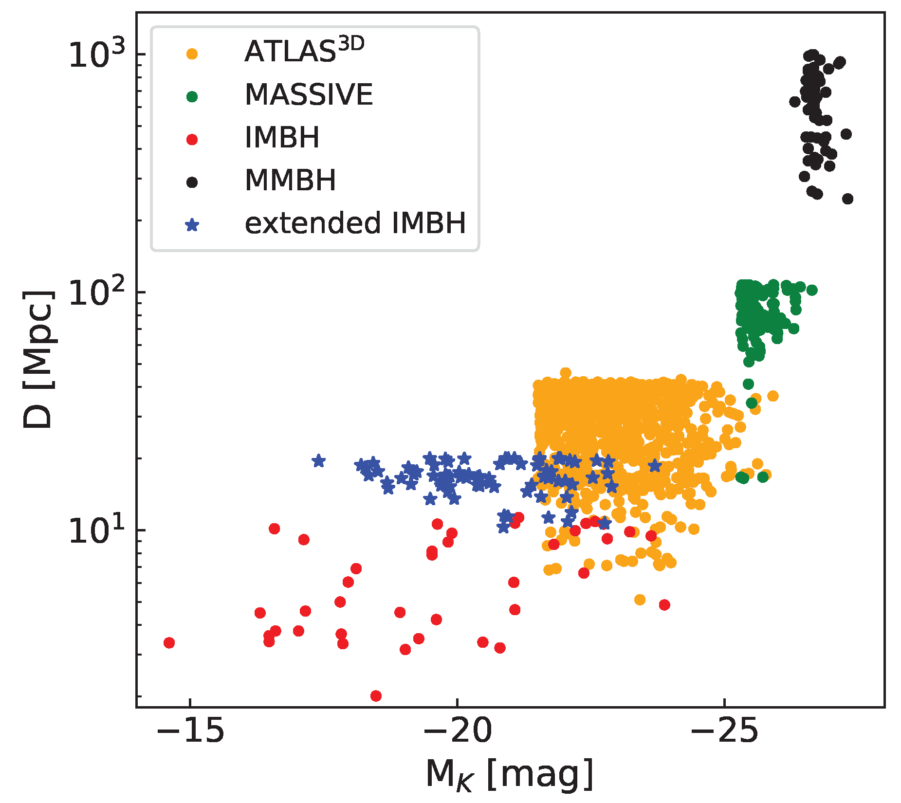
Figure 2.
Left: The – relation shows the correlation between galaxy mass and NSC mass across various Hubble types [41,54,109,116,126]. Right: The – relation illustrates the connection between galaxy mass and the NSC’s effective radius [5,28,53,107]. For comparison, we included the 10 Mpc HARMONI IMBH sample [106].
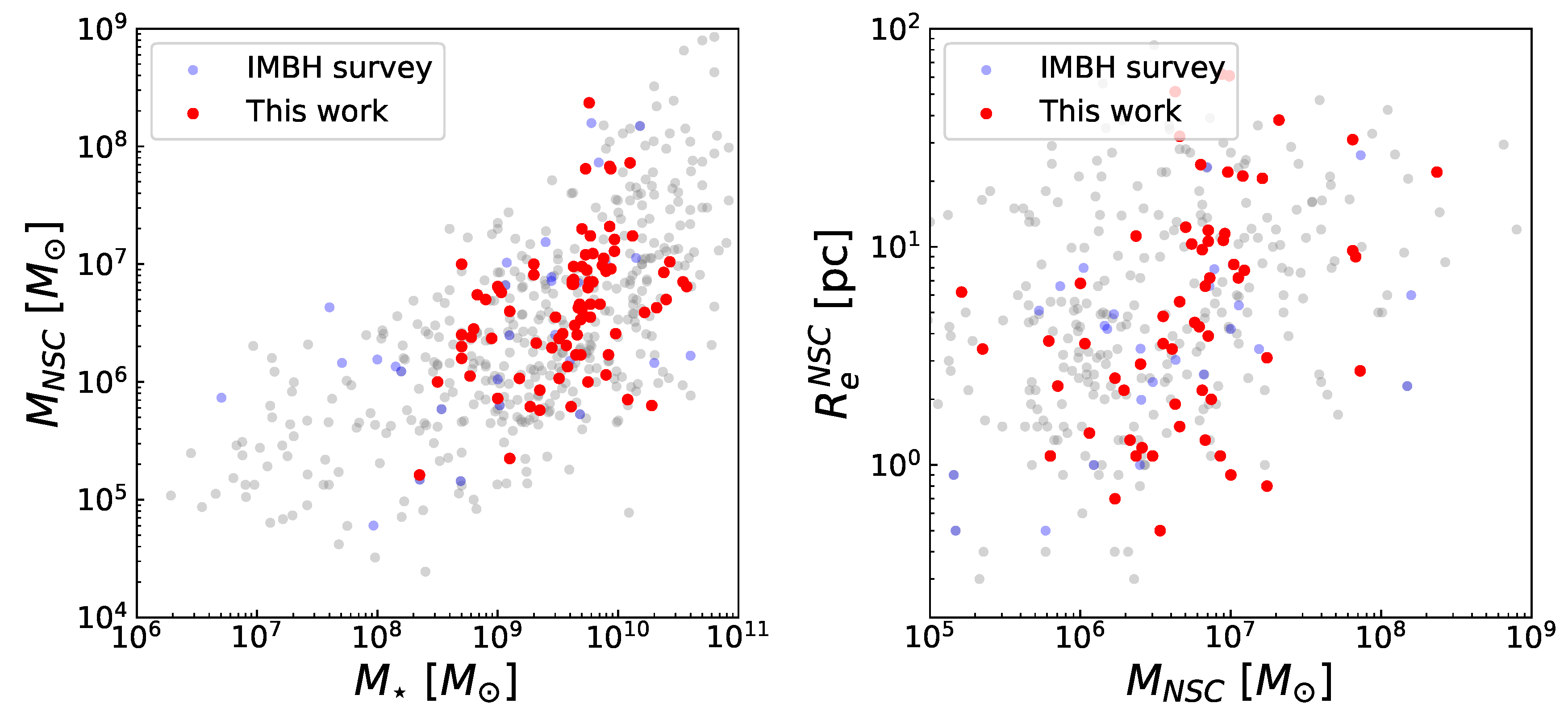
Figure 3.
Images from the HST, the Dark Energy Spectroscopic Instrument (DESI) Legacy Surveys DR10, The Two Micron All-Sky Survey (2MASS), and Sloan Digital Sky Survey (SDSS) of our extended HARMONI IMBH sample. Two red circles indicate radii of 12” (inner) and 60” (outer) from the galaxy center, marking the optimal region for selecting NGSs for AO correction. These stars are indicated by white crosses, with their respective H-band magnitudes estimated from Gaia.
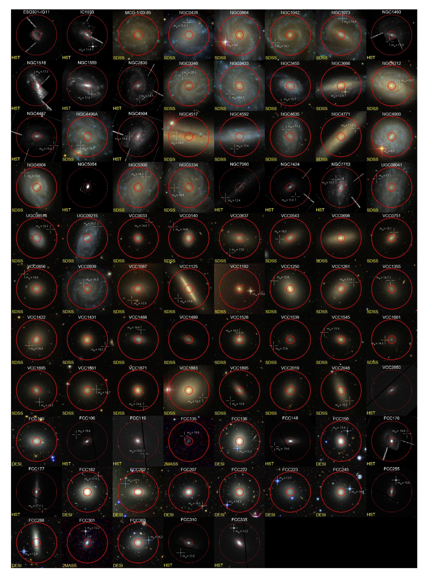
Figure 4.
Left: The HST/ACS WFC F850LP image of FCC 119 ( or kpc2) shows its large-scale morphology. Right: A zoom-in to the central region () highlights its NSC.
Figure 4.
Left: The HST/ACS WFC F850LP image of FCC 119 ( or kpc2) shows its large-scale morphology. Right: A zoom-in to the central region () highlights its NSC.
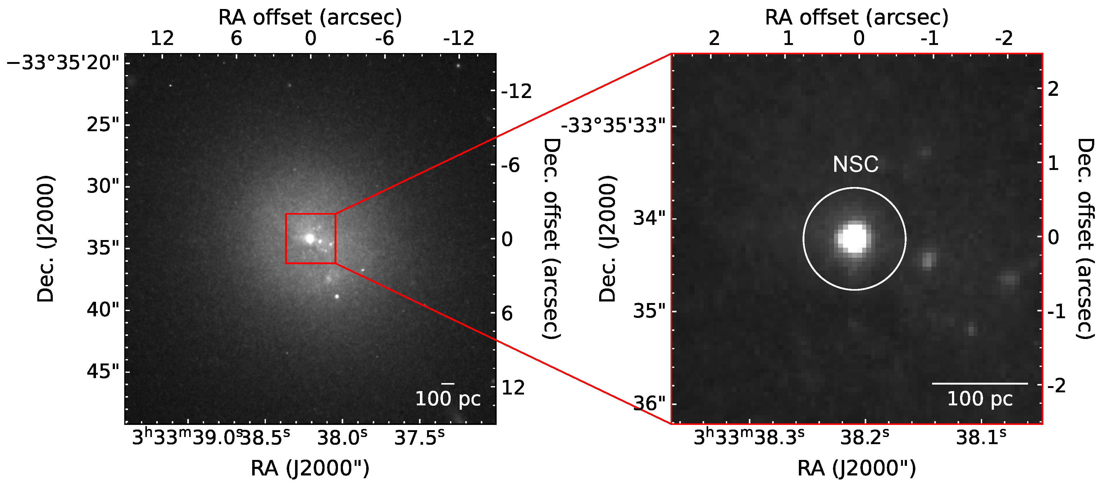
Figure 5.
Top: The HST ACS/WFC F850LP radial SB profile of FCC 119 (blue dots) is shown simultaneously with the best-fit model (purple-thick line), which is a combination of a core-Sérsic (red-dotted line) and a Sérsic (red-dashed line) function, extrapolated into both the unresolved region of and the extended region beyond 20″. The best-fit parameters of the best-fit model are shown in the legend. Bottom: The residual (data-model) between the SB and the best-fit combined function.
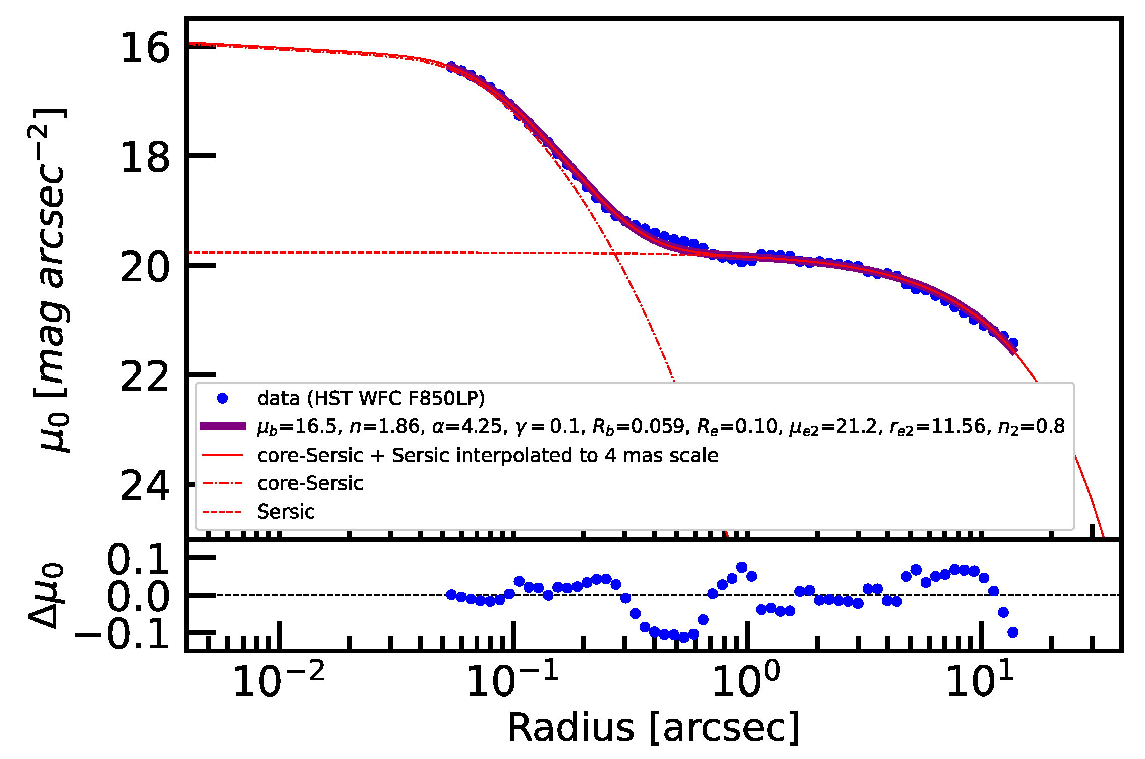
Figure 6.
The central Voronoi-binned spectra of FCC 119 are presented for the three mock IFS data cubes generated by HSIM (black), along with their best-fit pPXF models (red). The residuals, calculated as (data-model), are shown as green points.
Figure 6.
The central Voronoi-binned spectra of FCC 119 are presented for the three mock IFS data cubes generated by HSIM (black), along with their best-fit pPXF models (red). The residuals, calculated as (data-model), are shown as green points.
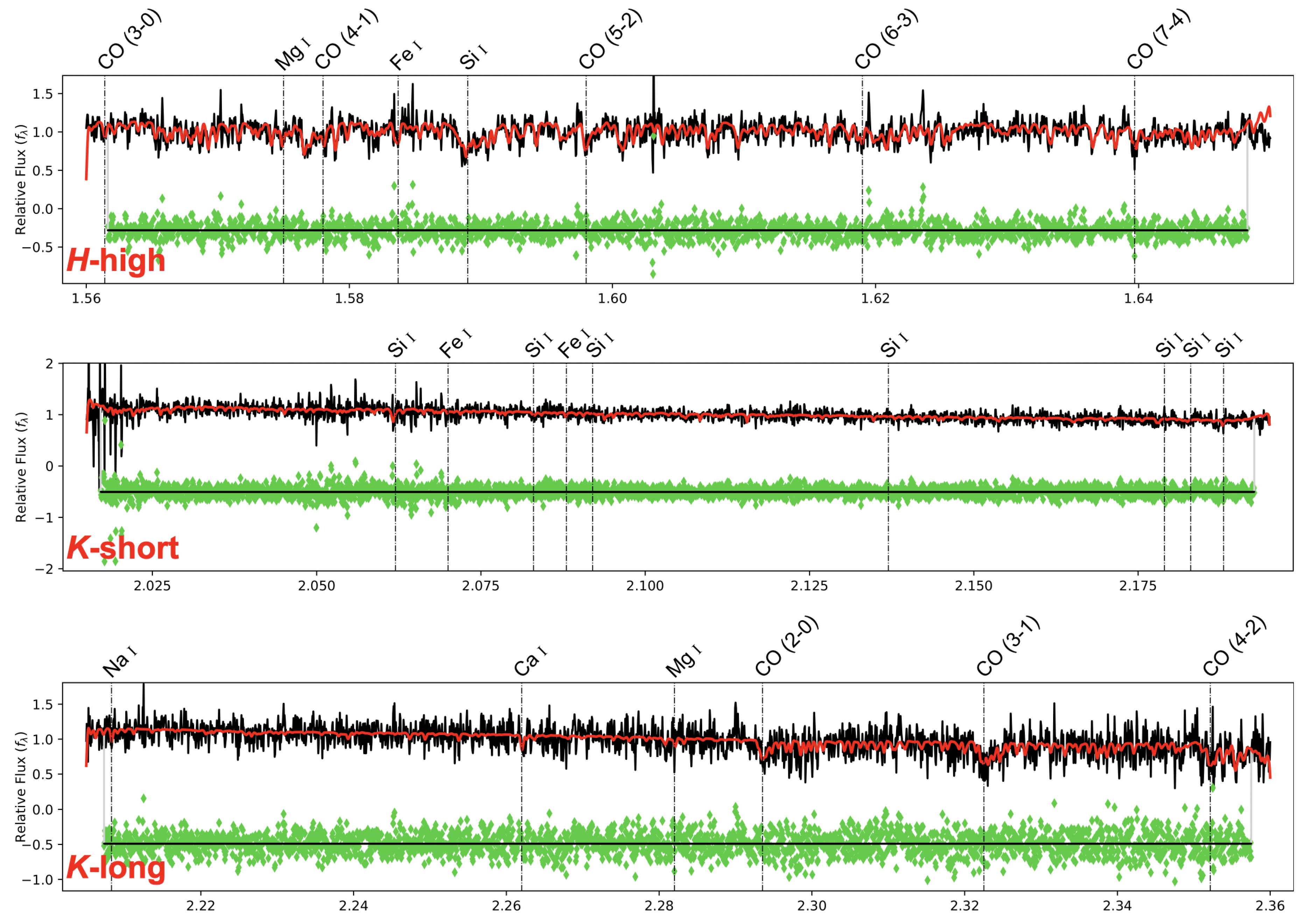
Figure 7.
The 2D stellar kinematic maps of FCC 119, derived from the three mock IFS gratings, show the velocity (V, left), velocity dispersion (, middle), and root-mean-square velocity (, right). The black contours in each map represent isophotes extracted from the collapsed mock IFS cubes, decreasing in brightness by 1 mag arcsec−2 from the center outward. For each mock IFS grating, the kinematic maps were simulated assuming no BH (top) and including an IMBH (bottom).
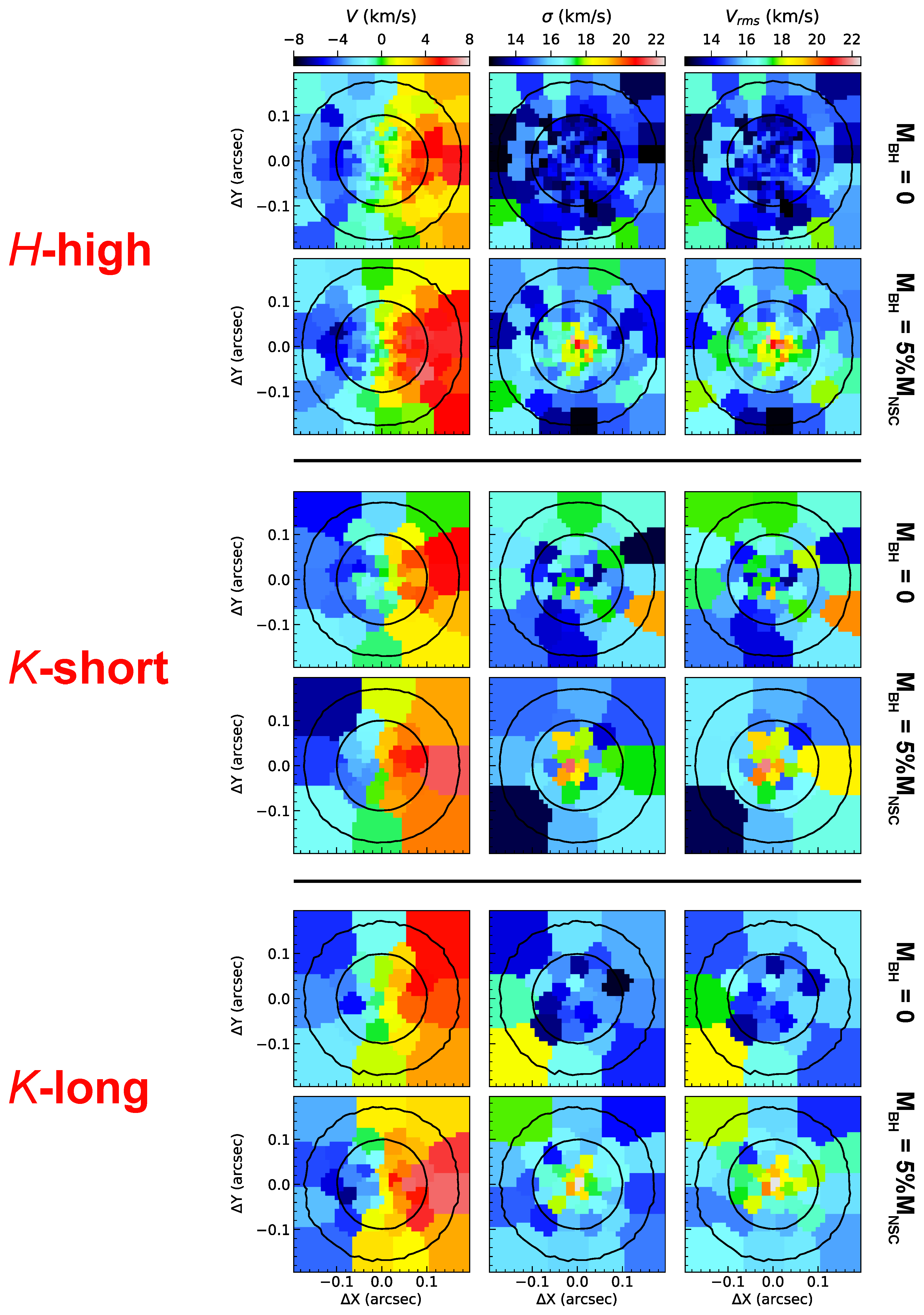
Figure 8.
The PDF of four parameters (i, , , ) constrained using JAM within the AdaMet MCMC optimization framework, derived from mock H-high IFS data cubes. The figure presents results for two different cases: no BH (left) and 5% (right). Each data point in the 2D scatter plots represents a single model, with colors indicating the log-likelihood. The 1D histograms above display the corresponding projected 1D distributions. In the upper-right corner, a comparison is shown between the mock kinematic maps and their best-fitting model.
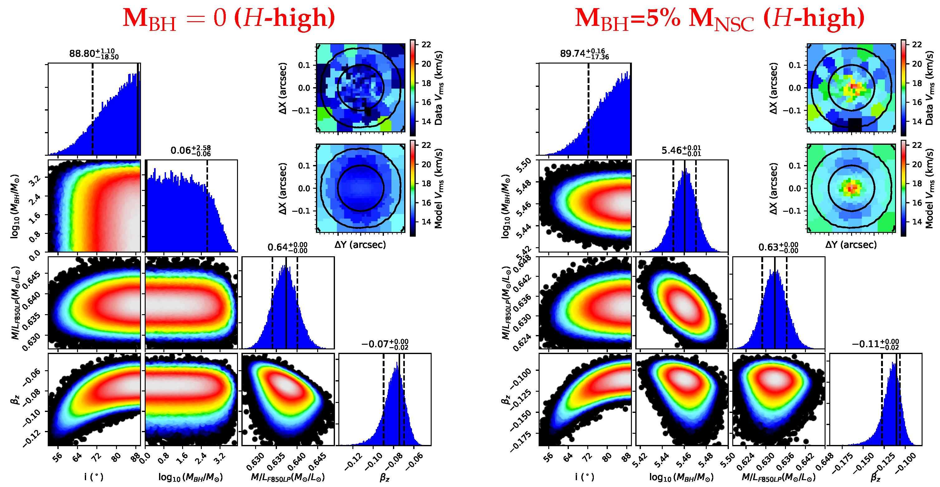
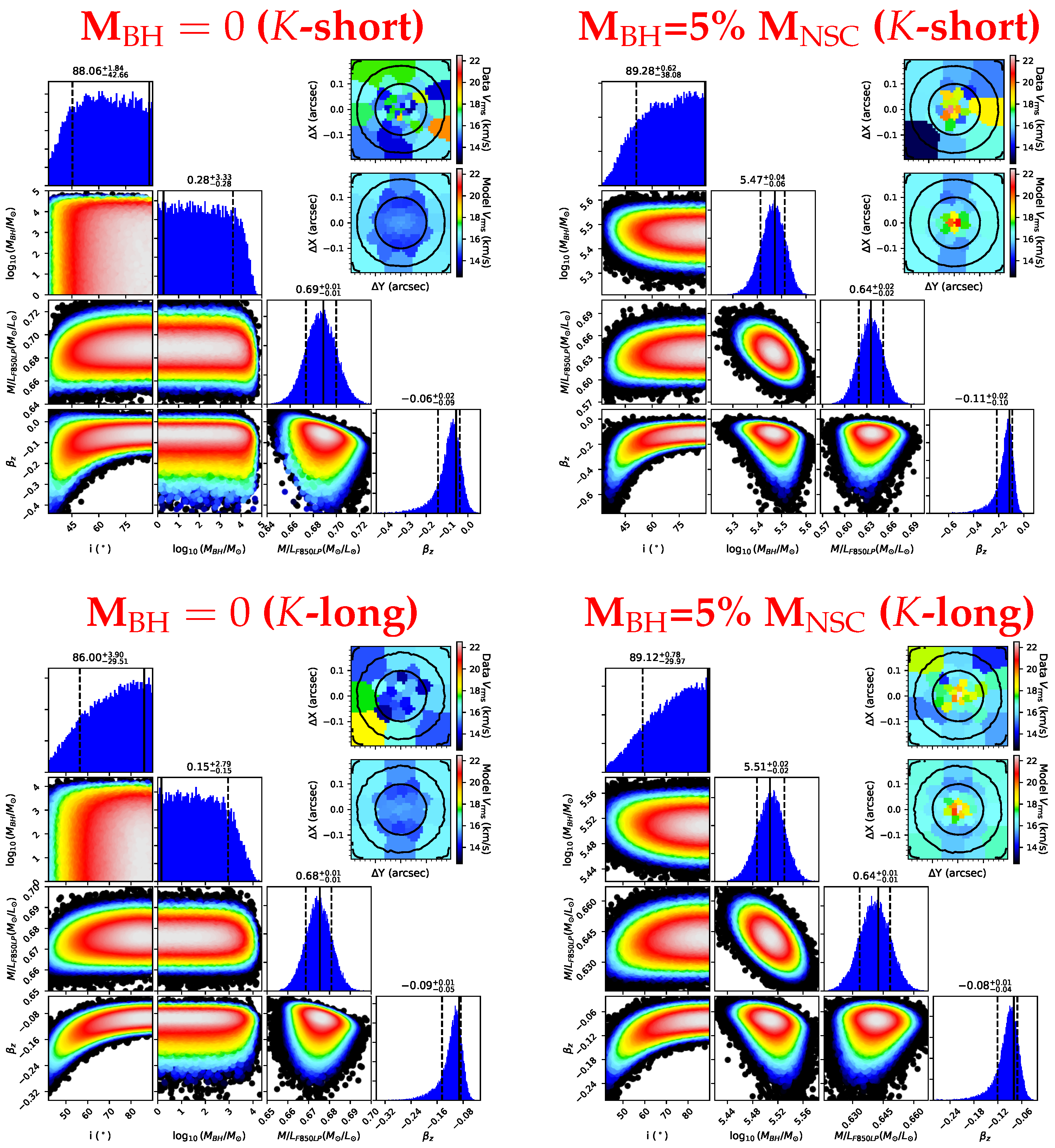
Figure 10.
A comparison of the input used in HSIM and the recovered values within CL. The black dashed line represents the line of equality between the input in HSIM and our recoveries.
Figure 10.
A comparison of the input used in HSIM and the recovered values within CL. The black dashed line represents the line of equality between the input in HSIM and our recoveries.
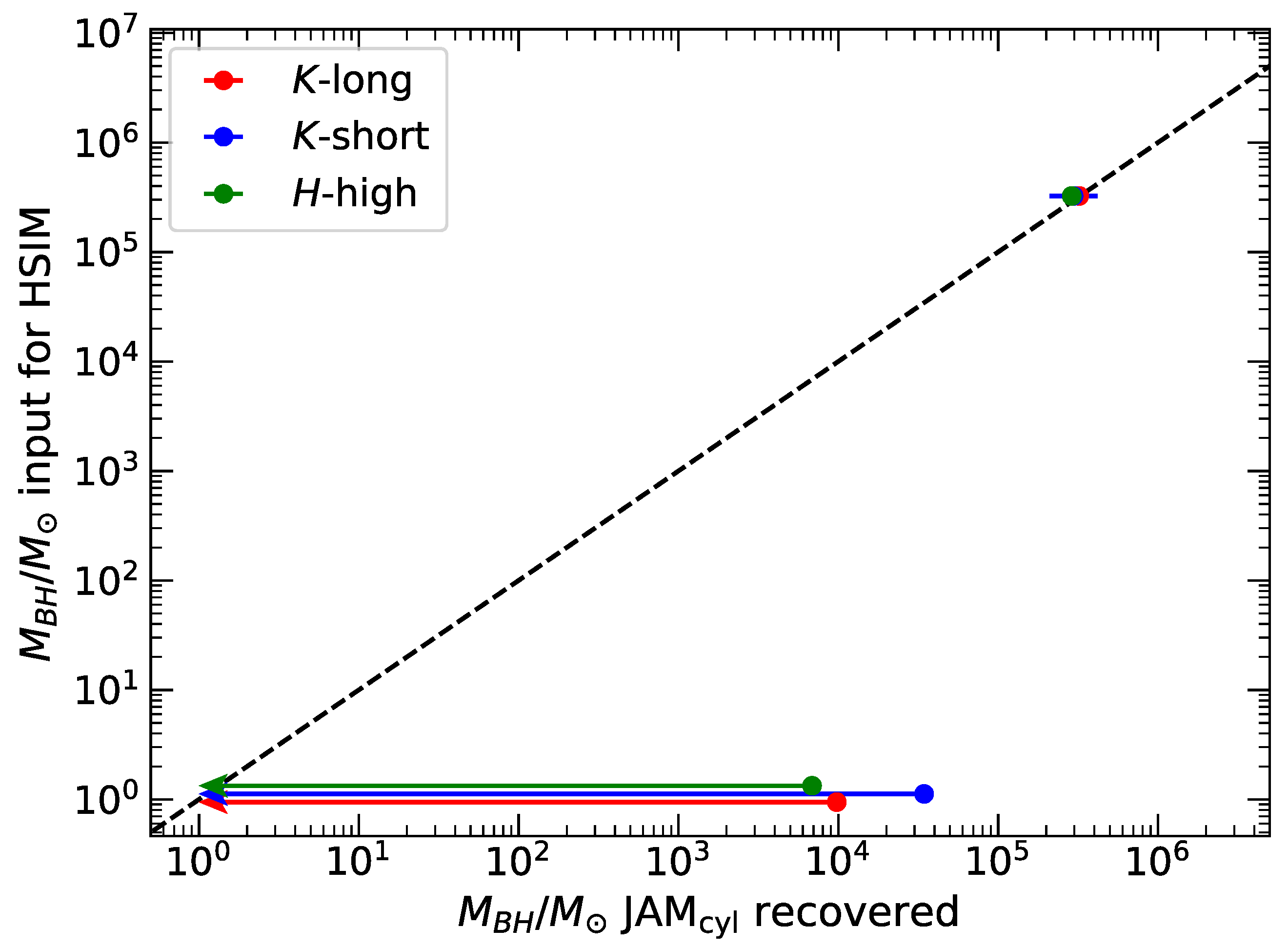
Figure 11.
Relaxation time (trelax) as a function of radius plots along the semi-major axis of FCC 119 (black-solid line). The red dash-dotted line indicates the effective radius of its NSC ()
Figure 11.
Relaxation time (trelax) as a function of radius plots along the semi-major axis of FCC 119 (black-solid line). The red dash-dotted line indicates the effective radius of its NSC ()
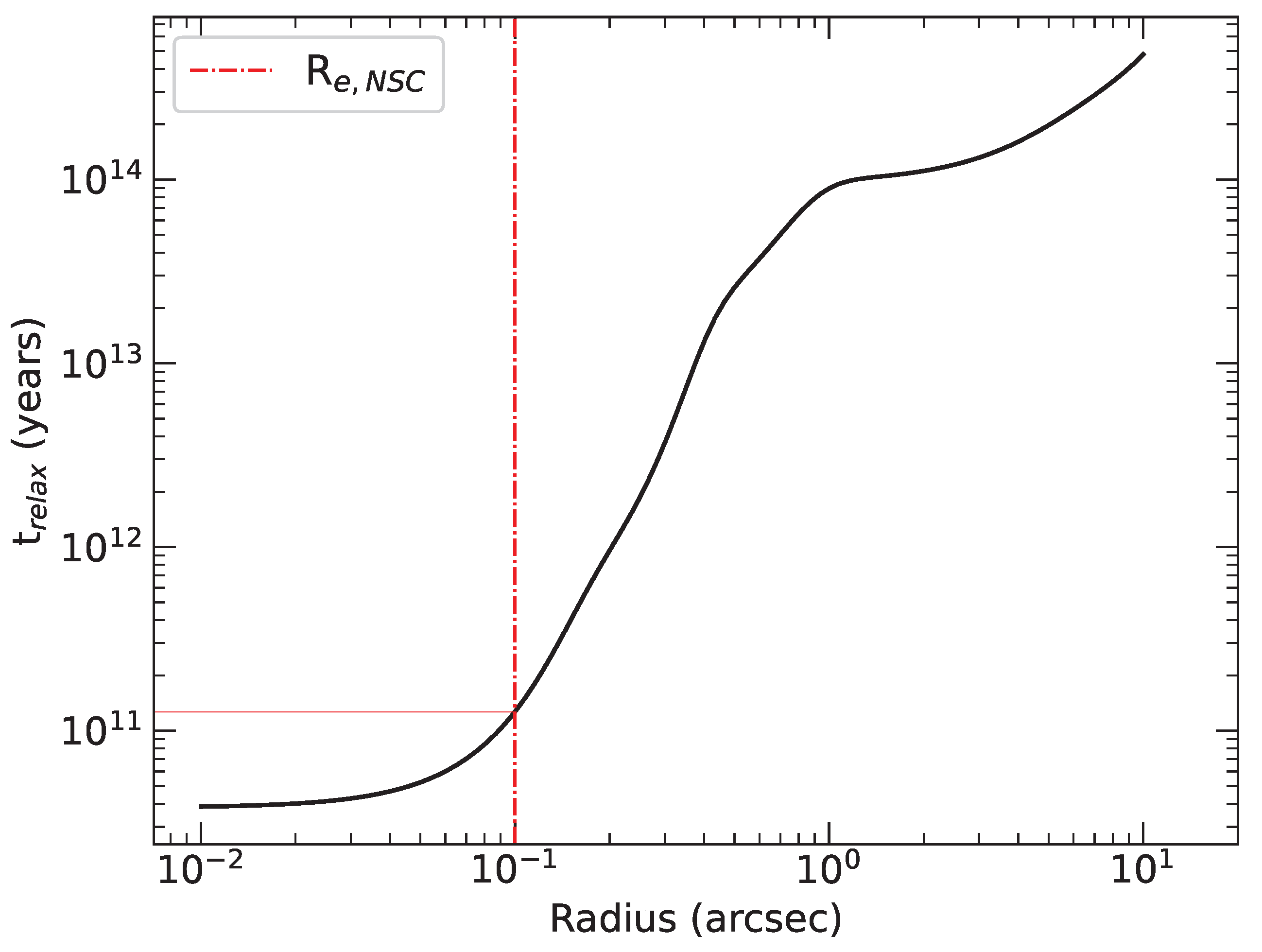
Table 1.
Selected criteria for dwarf galaxies
| ELT Observability: | |
| Galaxy zone of avoidance: | |
| Central stellar-velocity dispersion: | km s−1 |
Table 2.
Properties of the selected sample
| Distant range: | Mpc |
| Galaxies -band absolute magnitude: | |
| Galaxy stellar mass range: | ≲ M★,gal |
| Effective : | kpc |
| NSC mass range: | |
| NSC effective radius: | pc |
Table 5.
The HST/WFC F850LP MGE model of FCC 119
| j | ( | ||
| (1) | (2) | (3) | (4) |
| 1 | 9428.31 | 0.060 | 1.00 |
| 2 | 2535.54 | 0.131 | 1.00 |
| 3 | 175.71 | 0.346 | 1.00 |
| 4 | 91.52 | 2.679 | 1.00 |
| 5 | 243.69 | 6.034 | 1.00 |
| 6 | 187.84 | 9.868 | 0.85 |
| 7 | 68.45 | 13.762 | 0.85 |
| 8 | 10.19 | 17.689 | 0.85 |
| 9 | 0.37 | 21.999 | 0.85 |
Notes: Columns in order: Gaussian component number, luminosity surface density, dispersion along the major axis, and axial ratios.
Table 7.
Best-fit JAM models and uncertainties.
| Initial | Input | ||||||
| parameters | JAM guess | best-fit | (16–84)% | (0.14–99.86)% | best-fit | (16–84)% | (0.14–99.86)% |
| (1) | (2) | (3) | (4) | (5) | (6) | (7) | (8) |
| H-high | |||||||
| i (°) | 65 | 89 | >19 | >36 | 90 | >17 | >34 |
| /M⊙) | (*) | 0.06 | <2.58 | <3.68 | 5.460 | ±0.010 | ±0.031 |
| (M⊙/L⊙) | 0.6 | 0.637 | ±0.003 | ±0.009 | 0.633 | ±0.004 | ±0.011 |
| 0 | −0.074 | ±0.010 | ±0.039 | −0.110 | ±0.011 | ±0.044 | |
| K-short | |||||||
| i (°) | 65 | 88 | >43 | >56 | 89 | >38 | >56 |
| /M⊙) | (*) | 0.28 | <3.33 | <4.37 | 5.472 | ±0.050 | ±0.150 |
| (M⊙/L⊙) | 0.6 | 0.689 | ±0.013 | ±0.039 | 0.636 | ±0.017 | ±0.050 |
| 0 | −0.057 | ±0.052 | ±0.240 | −0.114 | ±0.062 | ±0.340 | |
| K-long | |||||||
| i (°) | 65 | 86 | >30 | >48 | 89 | >30 | >50 |
| /M⊙) | (*) | 0.15 | <2.79 | <3.92 | 5.507 | ±0.022 | ±0.065 |
| (M⊙/L⊙) | 0.6 | 0.675 | ±0.006 | ±0.019 | 0.643 | ±0.008 | ±0.022 |
| 0 | −0.093 | ±0.029 | ±0.130 | −0.080 | ±0.025 | ±0.230 | |
Notes: Columns 1–2: The free parameters of JAM, their initial guessed values. The asterisk (*) in in Column 2 indicates that the initial guesses for the either zero or . Columns 3–5: the best-fitting parameters for the case without a central BH ( ), their 1 and 3 uncertainties. Columns 6–8: Same as Columns 4–5 but for the input .
Disclaimer/Publisher’s Note: The statements, opinions and data contained in all publications are solely those of the individual author(s) and contributor(s) and not of MDPI and/or the editor(s). MDPI and/or the editor(s) disclaim responsibility for any injury to people or property resulting from any ideas, methods, instructions or products referred to in the content. |
© 2025 by the authors. Licensee MDPI, Basel, Switzerland. This article is an open access article distributed under the terms and conditions of the Creative Commons Attribution (CC BY) license (http://creativecommons.org/licenses/by/4.0/).
Copyright: This open access article is published under a Creative Commons CC BY 4.0 license, which permit the free download, distribution, and reuse, provided that the author and preprint are cited in any reuse.


