Modified Field Reformation and Unified Gravity: The Theory of Everything and the Solution for Quantum Gravity

1. Introduction

Quantum Gravity and Black Hole behavior have been a century-long debate and mystery. Quantum gravity is the effort to unify Einstein’s theory of general relativity, which describes gravity on cosmic scales, with quantum mechanics, which governs the atomic and subatomic world. Despite decades of research, physicists have not yet formulated a complete, testable theory that simultaneously captures the quantum behavior of particles and the curved spacetime framework in which gravity is understood.

In this paper, we will present our quantum framework based on the Sophy-Peter mathematical framework [1], which explains the Hawking radiation formation process, perfectly solves the black hole information paradox, describes quantum particle trajectories and the wave function in spacetime, and describes their behavior near spacetime curvature and the behavior of black holes. In this framework, we describe spacetime as a discrete set of causal events and interactions based on wave functions and a set of rules instead of a smooth, continuous manifold.

The black hole information paradox arises when the principles of quantum mechanics are combined with the predictions of general relativity. According to general relativity, black holes are regions of spacetime where gravity is so strong that nothing (not even light) can escape. However, in the 1970s, Stephen Hawking used a semiclassical approach, applying quantum field theory to curved spacetime, and discovered that isolated black holes are not completely black. Instead, they emit a faint form of radiation, which suggests that black holes can slowly lose mass and eventually evaporate. To approach this paradox, our framework describes singularities not as infinitely dense curvatures that nothing can escape from, but as a state of very dense curvature whose value is the largest bounded number, denoted as "Y". The process of reaching the Y curvature includes a non-linear growth (which is a part of the framework), resulting in a form of radiation escaping the black hole, eventually leading to its evaporation.

Current quantum mechanics model and over-time equations (describing the behavior of subatomic particles) do not have an explanation for the force of gravity, nor the trajectory of particles near dense curvatures, or at least the predictions give non-logical results. Although we know that equations like Schrödinger’s give us fair results that we can trust on a certain level, even using the current standard model, we still cannot get a theory of everything, so we assume that these equations are not complete, and that is the reason we cannot see the full picture. Spacetime behaves according to a set of certain rules (which will be described later) that cause the evolution of wave functions after their interactions, which we observe as gravity. Along with the spacetime rules, we fulfilled the missing parts in the time-dependent equations for the trajectory of particles, making them compatible with our framework and getting accurate predictions of particles’ behavior near dense curvatures.

2. SP Framework (Sophy-Peter Mathematical Framework)

Before we move to physics equations, we have to explain the new paradigm of number interpretation that was described in detail in our previous paper [1]. It is called the Sophy-Peter mathematical framework (we will say SP in the future to make it shorter).

First and most important is that we will interpret numbers as waves, which means it will allow them to have interference between each other. Later it will be explained how this is possible. Second, numbers have limits. We provide boundaries in the new number theory, which are the largest possible positive number with the notation "Y" and the smallest possible positive number "E". This will allow us to deal with singularities and avoid any paradoxes connected with infinity. Third, numbers aren’t actually growing linearly.

$$f(x)=x$$

The linear growth is present, but only on an interval. The increase is following the increasing function $f(x)=x$ which is:

$$f(x)={\displaystyle \frac{Y}{2}}{sin}^{-1}\left({\displaystyle \frac{x}{Y}}\right)+{\displaystyle \frac{x\sqrt{1-{\left(\frac{x}{Y}\right)}^2}}{2}}$$

(1)

After reaching the largest number the number line start to decrease but not the same way as it was increasing. Instead it is going to follow the decreasing function:

$$g(x)={\displaystyle \frac{Y}{2}}{sin}^{-1}\left({\displaystyle \frac{x}{Y}}\right)-{\displaystyle \frac{x\sqrt{1-{\left(\frac{x}{Y}\right)}^2}}{2}}$$

(2)

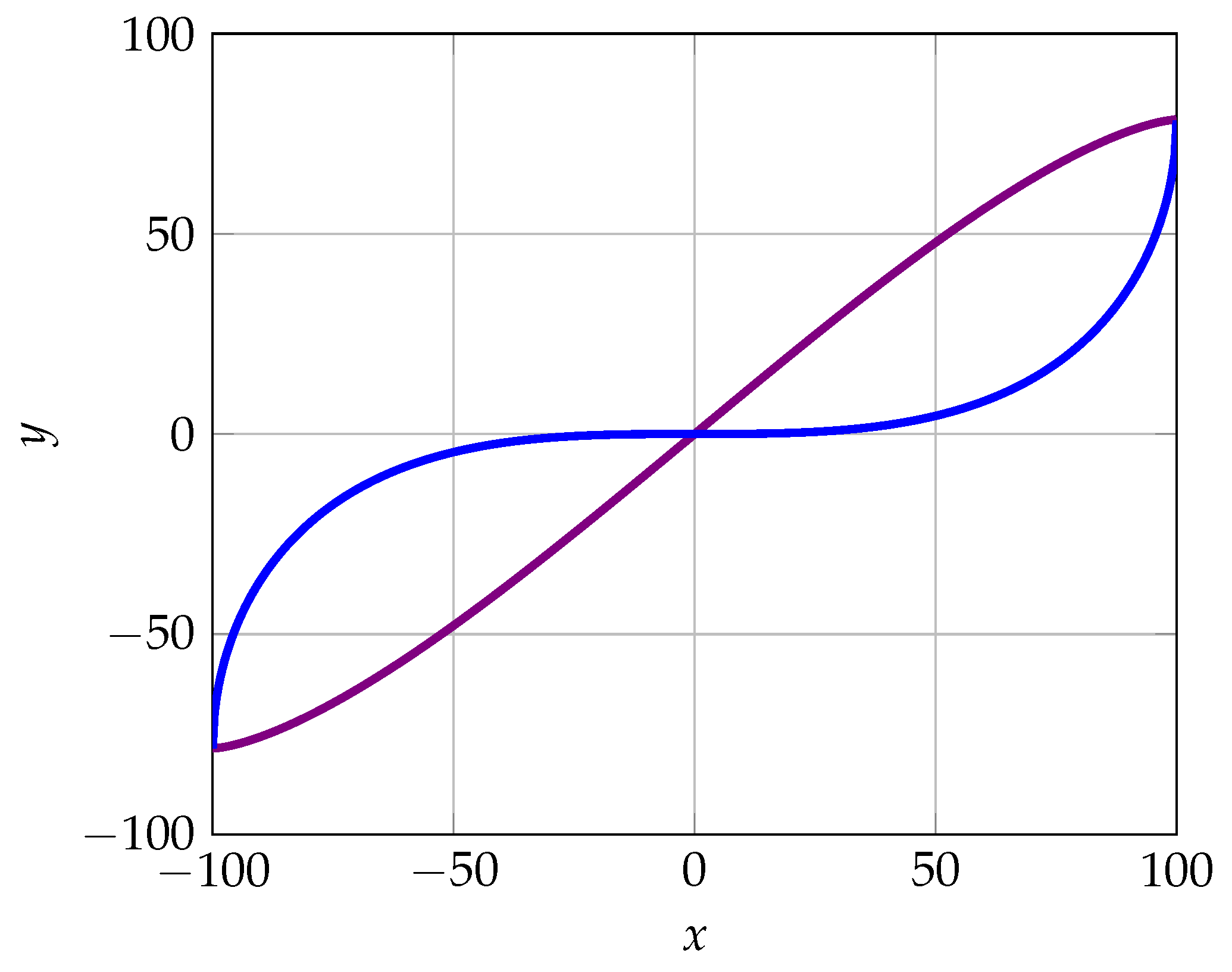
The visualization of both function will look as follows:

From the graph we can see the area between increasing and decreasing functions. This area is the area of number interference. We can describe the phenomenon of number interference as follows:

$$M_p=\left\{\begin{array}{cc}{\displaystyle \frac{p}{2lo{g}_2{(Y)}^2}}\hfill & ifpmod2=0\hfill \\ e^{{(-1)}^{{\displaystyle \frac{1}{2}}}\pi }\hfill & else\hfill \end{array}\right.$$

(3)

where p is the interference factor. The difference/ratio between the area of 2 given function within the increasing function.

The derivatives of increasing and decreasing functions are the following equations:

$$f^{\prime }(x)=\sqrt{1-{({\displaystyle \frac{x}{y}})}^2}$$

(4)

$$g^{\prime }(x)={\displaystyle \frac{x^2}{Y}}·{\displaystyle \frac{1}{Y\sqrt{1-{(\frac{x}{y})}^2}}}$$

(5)

If we went deeper into the properties of $f^{\prime }(x)$ and $g^{\prime }(x)$ we will find that they behave the same way as the original formulas Einstein relativity are build on, which speaks to the behavior of the universe.

Figure 1. The behavior of the functions, where the purple line is increasing function $f(x)$ and blue line is decreasing function $g(x)$.

Figure 1. The behavior of the functions, where the purple line is increasing function $f(x)$ and blue line is decreasing function $g(x)$.

Since in this framework the biggest number possible is Y, we can conclude that the smallest possible is ${\displaystyle \frac{1}{Y}}$ which we refer to as E. This number is the smallest number that can exist after 0 and the smallest fraction that can ever exist.

2.1. Dealing with "Infinite" Series

To explain how this can be done for any infinite series, let’s take the simplest divergent series, which sums all natural numbers ${\sum }_n^{\infty }n$. The first step we need to consider is writing the series in terms of $f(n)$.

$$n\to f(n),\sum _n^{Y}f(n)$$

$$\sum _n^{-Y}g(f(Y)+f(n))$$

Then we will apply the interval of Y and $-Y$, and since this series continues beyond Y, it will transform to the decreasing function, creating interference between both. We can write the summation as:

$$N={\int }_{-Y}^{Y}M+f(x)dx+{\int }_Y^{-Y}M+g(x)dx$$

Where M is the interference variable added due to the fact that this series, unlike the other series Z which always stayed at 0, actually continued after $f(Y)$, which is on the decreasing function, until $-Y$. Thus, we take the difference between the areas under their curves, considering the interference between them.

2.2. New Series Summation Interpretation

To continue representing the summation of any series, we need to classify series into two categories: divergent and convergent. Since it is not infinite, we need to redefine these two terms:

Divergent: A series S with a function $S(x)$ where $S(Y\to f(Y))\neg \approx 0$, and the series attempts to keep increasing, eventually reverting to the decreasing function until $-Y$, when the interval of infinity ends. This results in interference, ending with a finite value representing the difference in areas between the curves.

Convergent: A series S with a function $S(x)$ where $S(Y\to f(Y))\approx 0$. Consequently, it does not surpass Y, which implies that we can assign a finite value to it, and it will not transition to the decreasing function.

Example

To see how to deal with convergent series, we will consider a famous convergent series S, written as

$$S=\sum _n^{\infty }{\displaystyle \frac{1}{n^2}}$$

As before, we need to rewrite the sum in terms of $f(n)$ due to the non-linear growth. It will be written as:

$${\displaystyle \frac{1}{n^2}}\to {\displaystyle \frac{1}{f{(n)}^2}}$$

To prove it is convergent, we need to test its behavior at $x=Y$. Before this, let’s define $s(x)$:

$$s(x)={\displaystyle \frac{1}{f{(x)}^2}}$$

Then let’s evaluate $s(Y)$:

$$s(Y)={\displaystyle \frac{1}{"f{(Y)}^2"}}={\displaystyle \frac{1}{"(\frac{\pi }{4}Y)2"}}={\displaystyle \frac{1}{\frac{{\pi }^2}{16}"Y^2"}}$$

To compute $"Y^2"$, which is also $"Y\times Y"$. It is worth noting that $"Y\times Y"|>Y$:

$$"Y\times Y"=g((Y)Y{\displaystyle \frac{d}{dY}}f(Y)+(Y\mathrm{mod}2)Y)$$

$$\because Y\to odd,\therefore Y\mathrm{mod}2=1⟶2$$

$$\therefore "Y\times Y"={\displaystyle \frac{\pi }{4}}Y$$

(6)

For further proof you can refer to [2].

Therefore we can continue evaluating $s(Y)$ from our knowledge we gained from Equation (6):

$$s(Y)={\displaystyle \frac{1}{\frac{{\pi }^2}{16}"Y^2"}}={\displaystyle \frac{1}{\frac{{\pi }^2}{16}"Y\times Y"}}={\displaystyle \frac{1}{\frac{{\pi }^2}{16}\times \frac{\pi }{4}Y}}={\displaystyle \frac{1}{\frac{{\pi }^3}{64}Y}}={\displaystyle \frac{64}{{\pi }^3}}{\displaystyle \frac{1}{Y}}$$

We know that E is the smallest positive integer, which almost converges to 0, written as:

$${\displaystyle \frac{1}{Y}}=E$$

Subsequently we can further evaluate $s(Y)$ to see if it converges to 0:

$$s(Y)={\displaystyle \frac{64}{{\pi }^3}}{\displaystyle \frac{1}{Y}}={\displaystyle \frac{64}{{\pi }^3}}E\approx 2E\approx 0$$

(7)

Therefore we proved that this series in convergence in our framework and can be written without the decreasing function as the sum of of integers from $s(1)$ to $s(Y)$ as:

$$S=\sum _n^Y{\displaystyle \frac{1}{f{(n)}^2}}={\displaystyle \frac{{\pi }^2}{6}}$$

(8)

To write a complete function that accounts for all small numbers using both the increasing and decreasing functions, we can use $\zeta (2)$. However, since this series converges, there is no need. Nonetheless, $\zeta (2)$ is written as:

$$\zeta (2)={\int }_{-Y}^{Y}M+f{(x)}^{-2}dx+{\int }_Y^{-Y}M+g{(x)}^{-2}dx$$

$$={\int }_{-Y}^{Y}M+{\displaystyle \frac{1}{{\left(\frac{Y}{2}{sin}^{-1}\left(\frac{x}{Y}\right)+\frac{x\sqrt{1-{\left(\frac{x}{Y}\right)}^2}}{2}\right)}^2}}dx+{\int }_Y^{-Y}M+{\displaystyle \frac{1}{{\left(\frac{Y}{2}{sin}^{-1}\left(\frac{x}{Y}\right)-\frac{x\sqrt{1-{\left(\frac{x}{Y}\right)}^2}}{2}\right)}^2}}dx$$

$$={\int }_{-Y}^Y{\displaystyle \frac{Mf{(x)}^2+1}{{\left(\frac{Y}{2}{sin}^{-1}\left(\frac{x}{Y}\right)+\frac{x\sqrt{1-{\left(\frac{x}{Y}\right)}^2}}{2}\right)}^2}}dx+{\int }_Y^{-Y}{\displaystyle \frac{Mg{(x)}^2+1}{{\left(\frac{Y}{2}{sin}^{-1}\left(\frac{x}{Y}\right)-\frac{x\sqrt{1-{\left(\frac{x}{Y}\right)}^2}}{2}\right)}^2}}dx$$

For "divergent" series solving example go to our previous scientific paper [1].

3. Theory

3.1. Particle Movement

Behavior of elementary particles is actually deterministic, since pure non-determinism or randomness is possible only with the existence of infinity [2]. This statement implies that it is possible to predict the behavior of the particles.

Since in the Sophy-Peter mathematical framework, the existence of infinity is prohibited, it is reasonable to use it for the particle movement equation.

We formulated the particle movement equation to be dependent on time and a set of variables (energies, temperature, tensors, etc.) with a deterministic wave function, so it is consistent. The set of variables depends on the case, but let us give some examples. Around the black hole, the photon’s variables are the energy, the space curvature, and the black hole temperature. In the case of qubits (bits of information in quantum computers), which are superconductors, they would be the potential and kinetic energies, environment temperature, and the current magnetic field around it. For the formulation of the particle movement equation, we used the Schrödinger equation and applied a variable-determined Hamiltonian within the bounds of the Sophy-Peter framework and its rules of interference, integrals, differentiations, and non-linearity.

How to determine particle movement itself? First of all, we should understand that spacetime isn’t linear. Unlike Einstein’s theory, every dimension follows the framework curve initially. More about spacetime will be described later. The next step is to build the loop of events that happens all the time and determines the particle movement.

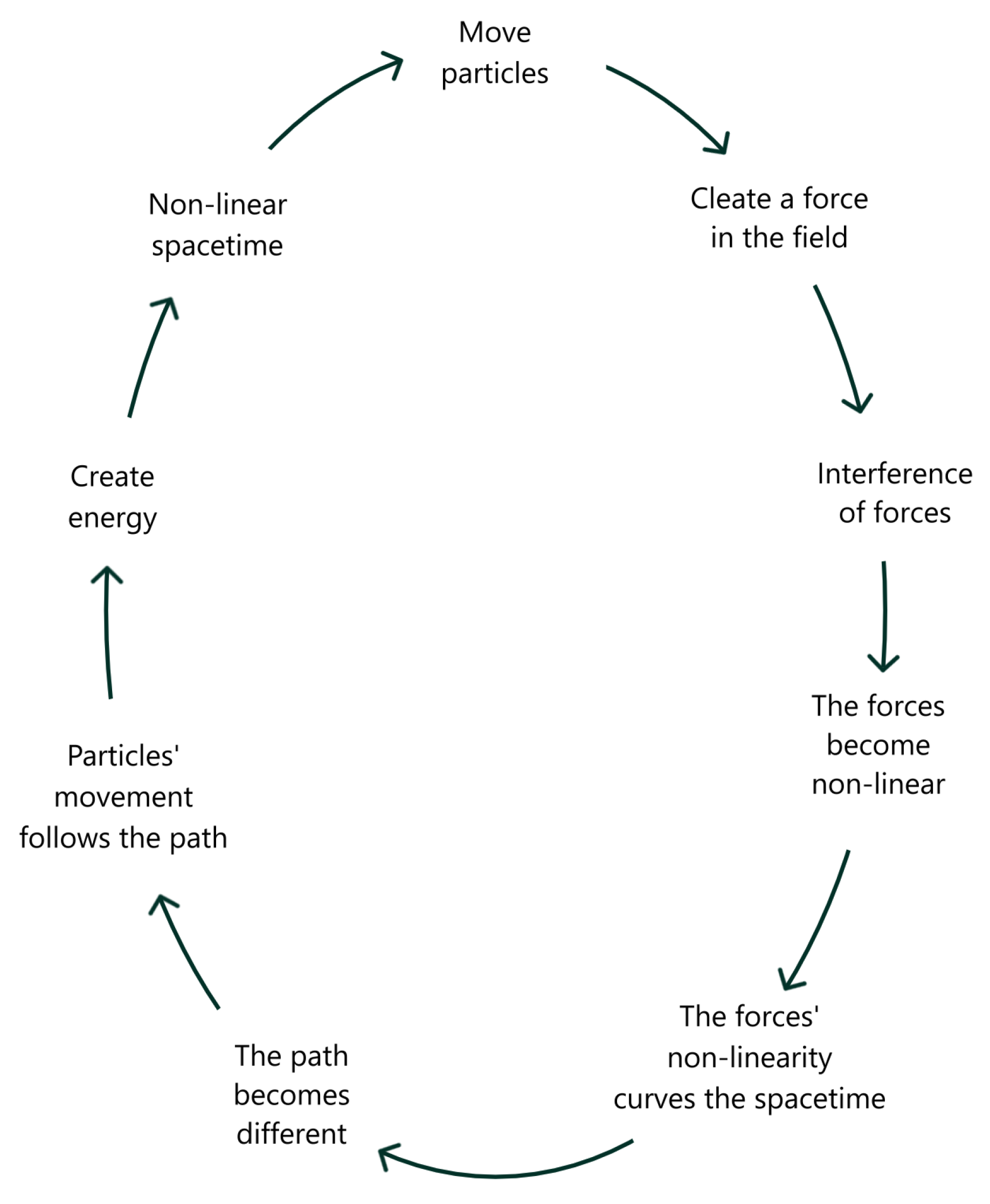
So we have a particle. The particle curves the field, the field creates the force, the force is not the same as the particle mass, which creates non-linearity, and that is where interference happens. And now spacetime is curved in a new way. Then particles move following the spacetime curvature, which is not the same path that would be calculated using the particle’s mathematics, so not a flat or a straight way. That is a non-linear path that came from the field and force.

From all of that, we can make a loop.

Figure 2. The Great Loop of Forces.

Figure 2. The Great Loop of Forces.

3.2. Spacetime

Spacetime contains three dimensions and time. With each dimensionality increase, the possible maximum decreases. Also, it is discrete. Actually, on a more abstract level, we can conclude that if we have a global maximum, it implies that something is discrete. Because of simple logic, which is: how do we represent the smallest possible number if we have a maximum? Simple — divide 1 by the maximum.

If someone asks, why can’t we divide one-half by the maximum and get a smaller number? The logic is simple: when we divide by the biggest number, we get a fraction. If we take one-half, which is the same as ${\displaystyle \frac{1}{2}}$, it implies we have to multiply the maximum by 2, which is nonsense due to the nature of a maximum. And since there is a minimum, it implies that it is discrete.

We also formulated that spacetime is a compact, finite-dimensional set of discrete points in time. We derive the curvatures with a geometrical approach where gravity is a force unified with the other three forces of nature. So we are saying that spacetime isn’t made of gravitons, but rather discrete points of particle interaction within a coherent framework.

3.3. Paradox of singularity

For a long time, after the concept of black holes was invented and then actual space objects were discovered, it was considered that the singularity, i.e., the center of a black hole, is infinite. But after Hawking radiation was discovered, it created a paradox: how can anything escape a black hole if the singularity is infinite, which means matter never reaches the center and definitely cannot escape the black hole? There were some theories to explain it, but they either collapsed, due to invalid results after calculations or contradictions, or were never proven.

The theory and math we are going to present make infinity forbidden, which removes all the paradoxes. Moreover, the existence of Hawking radiation becomes reasonable, and most important is that the computational results match the actual observations. The results will be presented later in the section with simulations.

3.4. How does matter interact with a black hole and why does it escape?

To answer the question of this section from the theoretical point of view, first of all, we have to recall the new number theory. As it was described in chapter Section 2, numbers are growing non-linearly, following the increasing function $f(x)$ until they reach "Y" (the maximal possible number); then they start to go the other way, following the decreasing function $g(x)$.

Also, we would like to recall the most important paradox, whose solution will be explained in the next paragraph. The black hole information paradox arises from a conflict between quantum mechanics and general relativity. While general relativity implies that information falling into a black hole is lost, quantum mechanics requires that information is preserved. Hawking radiation appears thermal and "random" (we know it isn’t actually random, as we described in the particle movement section ??), suggesting information loss as the black hole evaporates — a violation of unitarity in quantum theory. Resolving this paradox is central to unifying gravity with quantum mechanics.

Assume we describe space curvature in the black hole. From the number theory, we know that there is no infinity, so the maximal curvature of the space is equal to Y. We know from the particle movement chapter ?? that the particles follow the space curvature, which means that, first of all, they will follow the increasing function $f(x)$, and after reaching the singularity, they will go the other direction, following the decreasing function $g(x)$, until they leave the gravitational force of the black hole. The functions have very different curvatures, which is directly connected with the speed of particles’ movement, which explains why the speed of absorption of matter by the black hole is faster than the evaporation or Hawking radiation emission.

3.5. Photons around the black hole

In the black hole we have a photon sphere (sphere where photons initially start) and the distance (radius) from the center of the black hole (singularity) is

$$R={\displaystyle \frac{3GM}{c^2}}$$

Currently, the assumptions are that photons follow the space-time curvature and end up being destroyed in the infinite singularity. In our framework, we redefined the singularity, so obviously, the photons remain.

Around the black hole, there are forces and masses that are creating curvatures of space-time in the way we described, and the black hole mass itself. They all are creating interactive forces that determine the geometry of the black hole.

A photon that falls into a black hole in the photon sphere will follow the non-linear path (which follows the increasing function and creates the entering spiral) created by the black hole geometry and eventually ends up in the singularity point. After this, the photon will enter the exiting spiral, which is created by the black hole following the decreasing function, which has different properties for the photon. While exiting, its electromagnetic wave becomes expanded (red-shifted S) and it can be calculated by:

$$S=\sqrt{f^{\prime }(1-{\displaystyle \frac{2GM}{r_e{c}^2}})-g^{\prime }(1-{\displaystyle \frac{2GM}{r_e{c}^2}})}-1$$

Also the formula for time dilation:

$${\displaystyle \frac{dr}{dt}}=\sqrt{f^{\prime }(1-{\displaystyle \frac{2GM}{r{c}^2}})-g({\displaystyle \frac{2GM}{r{c}^2}})}$$

The difference between the entering and exiting spirals is interference of the spacetime.

After it became red-sifted and time dilated in the process spiral, it eventually escapes in another point of space time that it entered from, maintaining the same energy. It will be shown later in the simulation chapter.

4. Mathematics

4.1. SPBP

The core of black hole physics within the Sophy-Peter framework lies in a reimagined geometric structure, fundamentally changing the understanding of spacetime, as it points out that spacetime is characterized by a bounded curvature, an idea taken from the new interpretation of numbers. The line element $d{s}^2$, which defines the geometry of spacetime, is expressed as:

$$d{s}^2=g_{uv}(x)d{x}^{\mu }d{x}^v$$

This familiar formula present the redefinition within the metric tensor $g_{uv}(x)$, unlike standard general relativity where the metric components can vary, here $g_{uv}$ is defined as bounded, inhering the properties of the new number theory, this is represented as:

$$g_{uv}(x)=t_{uv}(x)cos({\displaystyle \frac{\pi }{2}}{\displaystyle \frac{x}{Y}})$$

Here $t_{uv}$ represents the conventional spacetime tensor for the physical propertied of time and energy. The term $cos({\displaystyle \frac{\pi }{2}}{\displaystyle \frac{x}{Y}})$ oscillates between -1 and 1. As the coordinate x approaches Y, the cosine term drives the metric towards 0, suggesting a phase transition in the geometry of the spacetime, this term also introduces a wave-like characteristic into the geometry itself.

4.1.1. Curvature Tensor

The concept of curvature which describes how spacetime bends and warps in the presence of mass and energy, given a set of $(\sigma ,\mu ,v)$ and a constant $\lambda$, the Riemann curvature tensor $R_{\sigma \mu v}$ is defined as:

$$R_{\sigma \mu v}=d_{\mu }{\mathsf{\Gamma }}_{v\sigma }-d_v{\mathsf{\Gamma }}_{\mu \sigma }+{\mathsf{\Gamma }}_{\mu \lambda }{\mathsf{\Gamma }}_{v\sigma }-{\mathsf{\Gamma }}_{v\lambda }{\mathsf{\Gamma }}_{\mu \sigma }$$

This definition for the Riemann tensor remains formally consistent with standard differential geometry, describing the non-commutativity of covariant derivatives. However, its foundation is altered by the underlying SPBP metric. The connection coefficients dictating how vectors change as they are parallel transported through spacetime, are defined as:

$${\mathsf{\Gamma }}_{\mu v}={\displaystyle \frac{1}{2}}{g}_{\lambda \lambda }(d_{\mu }{g}_{v\lambda }+d_v{g}_{\mu \lambda }-d_{\lambda }{g}_{\mu v})$$

It’s important to not the use of $g^{\lambda \lambda }$ in this expression, implies a summation over identical indices, this would be $g^{\lambda p}$ summed over p. Through the use of the metric tensor, the Riemann tensor, will inherit the non linear nature.

4.1.2. Scalar of Bounded Curvature

The scalar curvature R, a single value that characterizes the intrinsic curvature at any point in spacetime, is introduced in SPBP as a function of $m(x)$ in the increasing function $f(x)$:

$$R=f(m(x))$$

Here, $m(x)$ is a scalar quantity that emerges from the SPBP number interpretation, representing a form of effective mass influenced by the wave-like nature of numbers. The function f(x) is the increasing function from number theory, meaning that the scalar curvature’s behavior is directly tied to the non-linear, bounded progression of numbers.

4.1.3. Einstein Field Reformation

The profound redefinition of numbers and spacetime geometry requires a reformation of Einstein’s field equations, the cornerstone of gravitational theory. In SPBP, these equations take the form:

$$G_{uv}={\displaystyle \frac{8\pi G}{c^4}}{T}_{uv}(x)$$

While the overall structure resembles the classical Einstein field equations, relating spacetime curvature (the Einstein tensor) to the distribution of mass-energy (the energy-momentum tensor), the underlying definitions of both sides of the equation are fundamentally altered by the SPBP framework. The energy-momentum tensor $T_{uv}$, which traditionally describes the density and flux of energy and momentum, is no longer solely a classical quantity. In SPBP, it is redefined as:

$$T_{uv}=t_{uv}+\mathsf{\Theta }(x)f^{\prime (-1)}(\mathsf{\Theta })$$

Here, $t_{uv}$ can be considered the conventual classical component while the additional term introduces a new field that emerges, it signifies the inverse of the derivative of the increasing function with respect to the flux $\mathsf{\Theta }$

$$R_{uv}=g(m(x))ifm(x)>Y$$

4.2. SPBP Schwarzschild Geometry and Quantum Behavior of Black Holes

In the SPBP framework, the classical Schwarzschild geometry is generalized through the lens of bounded curvature and nonlinear number-theoretic metrics. The Schwarzschild solution, traditionally derived from Einstein’s vacuum field equations, is preserved in structure but modified in its mass term. Rather than a linear dependence on mass, SPBP introduces a nonlinear transformation $f(M)$ governed by the number-theoretic bounding function. The metric is expressed as:

$$d{s}^2=-\left(1-{\displaystyle \frac{f(M)}{r}}\right)d{t}^2+{\left(1-{\displaystyle \frac{f(M)}{r}}\right)}^{-1}d{r}^2+r^{2}d{\sigma }^2$$

Here, $f(M)$ is a bounded function of the black hole mass M, and the metric components oscillate and transition smoothly as $r\to f(M)$, introducing a modulated curvature into the geometry. This modification gives rise to novel thermodynamic and quantum properties not captured by classical general relativity.

4.2.1. Extrinsic Curvature and Surface Gravity

The surface gravity k, which plays a central role in black hole thermodynamics and Hawking radiation, is redefined using a bounded derivative expression:

$$k={\displaystyle \frac{\pi }{4}}{\displaystyle \frac{d}{dr}}\left(1-{\displaystyle \frac{f(M)}{r}}\right)$$

This expression introduces a curvature modulation dependent on the number-theoretic structure of f, and ties surface gravity to geometric oscillations encoded in the metric.

4.2.2. Entropy in Bounded Geometry

Entropy S in the SPBP black hole is not simply proportional to the horizon area, but is derived through an integral constrained by the bounded curvature of space. Specifically, entropy is accumulated radially from the center to the Schwarzschild radius $r_s=f(M)$, using a bounded measure:

$$S={\int }_0^{r_s}{\displaystyle \frac{r}{\sqrt{1-{\left(\frac{r}{Y}\right)}^2}}}dr$$

This formulation links entropy to the geometric bound Y, introducing a saturation mechanism for entropy accumulation. As r approaches Y, the integrand diverges, representing a natural upper limit imposed by the structure of spacetime. At the limit, entropy becomes:

$$S={\displaystyle \frac{f{(M)}^2}{\hslash G}}$$

This resembles the Bekenstein-Hawking area law but emerges from bounded geometry rather than a classical horizon area.

4.2.3. Temperature and Thermodynamic Relations

Temperature in SPBP is directly tied to the surface gravity k, as in semi-classical black hole thermodynamics. The relation takes the form:

$$T={\displaystyle \frac{\hslash k}{2\pi }}$$

Due to the bounded nature of k, this relation implies a maximal black hole temperature, preventing divergence and supporting the idea that black holes in SPBP avoid traditional singularities.

4.2.4. Interference and Black Hole Merging Behavior

When two bounded-mass fields $m_1$ and $m_2$ interfere (such as during a merger or quantum tunneling), the resulting total mass is not additive, but governed by:

$$m=f(m_1)+f(m_2)+M_p$$

Here, $M_p$ represents the Planck-scale interference correction term. This encapsulates the quantum geometry contribution during merging processes, preventing arbitrary mass accumulation and suggesting that the geometry itself enforces mass quantization.

4.2.5. Radial Instability and Geometric Restoring Force

The stability of a particle’s radial position within a bounded gravitational field follows a modified geodesic deviation, expressed as:

$${\displaystyle \frac{d^{2}r}{d{t}^2}}=-\Delta f(M)+\eta m$$

This introduces a competition between the non-linear mass-dependent gravitational pull and a restoring force tied to the field $\eta m$, which may originate from the geometry’s resistance to curvature gradients — hinting at a form of geometric elasticity.

4.2.6. Black Hole Evaporation and Time Evolution

Evaporation is described via a modified Hawking-like radiation equation, where the mass loss is not simply thermally driven, but bounded by a non-linear mass function $g(M)$:

$${\displaystyle \frac{dM}{dt}}=-\alpha g{(M)}^4$$

The lifetime of the black hole is then derived through a bounded integral over this mass function:

$$t={\int }_0^{M_0}{\displaystyle \frac{1-g^{\prime }{(M)}^2}{g{(M)}^4}}dM$$

This suggests a delay in evaporation near the Planck scale due to the bounded nature of g, avoiding the traditional singular end-state of complete evaporation.

4.2.7. Cosmological Core and Collapse Reversal

SPBP introduces a dynamic cosmological core through a bounded time-dependent function:

$$C(t)=Ytanh\left({\displaystyle \frac{t}{Y}}\right)$$

From this, the Ricci curvature evolves as:

$$R_c={\mathsf{\Lambda }}^{\mu \nu }C(t)$$

As $t\to t_e$, the curvature diminishes:

$$\underset{t\to t_e}{lim}R\to 0,d{s}^2\to {\delta }_{\mu \nu }$$

This reflects a geometric flattening at late times — black holes in SPBP may “cool” into a flat spacetime, encoding information instead of erasing it, supporting unitarity.

4.2.8. Information Retrieval and Inversion Principle

To retrieve information potentially encoded or lost during evaporation, SPBP introduces an inverse mass flow mechanism:

$$m(t)=G^{-1}\left({\displaystyle \frac{dM}{dt}}\right)$$

This inversion forms the foundation of an information reconstruction algorithm:

$$SP(x)=\int f^{-1}(R(x,t))M_{p}dx$$

This connects curvature evolution with informational recovery, suggesting that SPBP black holes are informationally transparent, with quantum information embedded in curvature patterns retrievable via bounded inversions.

4.2.9. Quantum Potential and Geodesics

The quantum potential for a massless particle (e.g., a photon) near the SPBP black hole is defined as:

$$V_{SP}(r)={\displaystyle \frac{1}{2}}\left(1-{\displaystyle \frac{f(M)}{r}}\right){\displaystyle \frac{L^2}{r^2}}$$

This governs the orbital stability, with the photon sphere at:

$$r_{\gamma }=arg\underset{r}{max}\left[V_{SP}(r)\right]$$

Geodesic motion is governed by:

$${\left({\displaystyle \frac{dr}{d\lambda }}\right)}^2+V_{SP}(r)=E^2$$

Bounded curvature leads to novel stable orbits and critical radii differing from classical Schwarzschild predictions.

4.2.10. Wave Equation and Quantum Oscillations

Scalar perturbations in the SPBP background obey a Schrödinger-like equation:

$${\displaystyle \frac{d^2\mathsf{\Psi }}{d{r}_{*}^2}}+\left[{\omega }^2-V_{SP}(r)\right]\mathsf{\Psi }=0$$

The quantized oscillation modes are given by:

$${\omega }_n={\displaystyle \frac{n\pi }{\mathcal{F}(M)}}-i{\gamma }_n$$

This implies discrete, damped quasi-normal modes whose spectrum depends on the bounded transformation $\mathcal{F}(M)$, providing a fingerprint for the underlying mass structure.

4.2.11. Spacetime Utility Function

To evaluate total curvature-weighted density across the geometry, SPBP introduces a utility function:

$$\mathcal{U}=\int \rho (x)·\tilde{\mathcal{R}}(x)dx$$

This measures the total bounded geometric utility of a spacetime region — akin to evaluating the information or energy compression within a space.

4.2.12. Quantum Field Representation

Finally, SPBP proposes a wavefunction of space encoded by:

$$\mathsf{\Psi }(x)=e^{i\pi ·f(x)/Y}$$

This oscillatory exponential defines the probability amplitude for geometry itself, suggesting that spacetime is quantized at the number-theoretic level, forming standing waves modulated by $f(x)$.

4.3. Unified gravity in the space time metric

4.3.1. Gauge Fixing

In the context of the SPBP framework, gauge fixing plays a critical role in defining the path integral quantization of fields, especially when dealing with electromagnetic and interacting gauge fields within a redefined number-theoretic spacetime [1,7,8]. To ensure the functional integral is well-defined, we introduce a gauge fixing condition consistent with the bounded curvature and modified geometric structure [9].

We begin by fixing the gauge via the identity:

$$e_v=\delta x_v=\delta X_v={\delta }_v$$

This ensures the local frame is aligned with the chosen gauge, effectively constraining coordinate redundancy. The determinant of the metric tensor, g, introduces the scalar factor $\sqrt{-g}$ into the functional measure, as is customary in curved spacetime [7].

The un-gauge-fixed functional integral over all field configurations is:

$$\int e^{iS[{\psi }^v,\psi ,A,H]}{D}_{{\psi }^v}{D}_{\psi }{D}_A{D}_H$$

where $\mathcal{D}$ denotes the functional integration over the corresponding field configurations. The action $S[{\psi }^{\nu },\psi ,A,H]$ is given by:

$$S[{\psi }^v,\psi ,A,H]=\int \mathcal{L}{d}^{4}x$$

with $\mathcal{L}$ representing the Lagrangian density for all interacting fields. We define a gauge condition function ${\mathcal{C}}_{\mathrm{em}}(A)$, chosen to reflect the SP dynamics [1]:

$${\mathcal{C}}_{\mathrm{em}}(A)=\sqrt{2{\mu }_0}{f}^{\prime }({\gamma }_b\theta A)$$

This expression encapsulates a derivative of the number-theoretic function f, scaled by coupling constants ${\gamma }_b$ and $\theta$, ensuring compatibility with the bounded spacetime geometry [1].

Under a gauge transformation parameterized by $\theta$, the electromagnetic field transforms as:

$$A_v(\theta )=A_v-{\displaystyle \frac{\hslash }{e}}{f}^{\prime }$$

where the transformation involves the derivative of the number function, linking gauge degrees of freedom with the bounded number space [1].

The auxiliary functional measure factor $D_e(x)$ is introduced via:

$$D_e(x)={\displaystyle \frac{1}{2d}}\left({\int }_{-Y}^{Y}f(xd)dx-{\int }_{-Y}^{Y}g(xd)dx\right)$$

capturing the difference between two modulated field functionals over the bounded domain $[-Y,Y]$ [1].

The functional integral, which incorporates gauge fixing and the Faddeev–Popov determinant, becomes:

$$\widehat{\delta }\left[C_{em}(A)\right]D_e\left(-{\displaystyle \frac{\hslash }{e}}{\partial }^2\right)\times e^{{\displaystyle \frac{i}{\hslash c}}S[\psi ,\overline{\psi },A,H]}\mathcal{D}\theta \mathcal{D}\overline{\psi }\mathcal{D}\psi \mathcal{D}A\mathcal{D}H$$

To express the functional delta function and the Faddeev–Popov determinant in this equation as Lagrangian density functionals, we rewrite:

$$\begin{array}{cc}\hfill \delta \left[{\mathcal{C}}_{\mathrm{em}}(A)\right]& =N_{\mathrm{em}}exp\left({\displaystyle \frac{i}{\hslash c}}\int {\mathcal{L}}_{\mathrm{em},\mathrm{gf}}^{\mathrm{mod}}{\mathrm{d}}^{4}x\right),\hfill \end{array}$$

(9)

$$\begin{array}{cc}\hfill {\mathcal{L}}_{\mathrm{em},\mathrm{gf}}^{\mathrm{mod}}& =-{\displaystyle \frac{1}{2{\mu }_0{\xi }_e}}{\left[{\mathcal{C}}_{\mathrm{em}}(A)\right]}^2{\displaystyle \frac{1}{f^{\prime }(x)}}\hfill \end{array}$$

(10)

The Faddeev–Popov determinant is expressed via a ghost field Lagrangian [4]:

$$det\left(-{\displaystyle \frac{\hslash }{e}}{\partial }^2\right)=\int exp\left({\displaystyle \frac{i}{\hslash c}}\int {\mathcal{L}}_{\mathrm{em},\mathrm{ghost}}^{\mathrm{mod}}{\mathrm{d}}^{4}x\right)\mathcal{D}{c}_{\mathrm{em}}\mathcal{D}{\overline{c}}_{\mathrm{em}}$$

$${\mathcal{L}}_{\mathrm{em},\mathrm{ghost}}^{\mathrm{mod}}=\hslash c·{\overline{c}}_{\mathrm{em}}\left({\partial }^2{c}_{\mathrm{em}}\right)·{\displaystyle \frac{1}{f^{\prime }(x)}}$$

This ghost Lagrangian enforces gauge symmetry at the quantum level and modifies the ghost propagator via the SPBP structure. The presence of the ${\displaystyle \frac{1}{f^{\prime }(x)}}$ factor in both gauge-fixing and ghost sectors highlights the essential role of the number-theoretic function f, embedding nonlinearity and boundedness into the quantum structure of gauge theory [1].

4.3.2. Gravity Gauge fixing

This replacement formally introduces the gauge constraint into the path integral and ensures that only physically distinct gravitational configurations contribute to quantum amplitudes. The appearance of $f(x)$ and $f^{\prime }(x)$ in this expression signals that the geometry of spacetime actively participates in regulating gauge redundancy.

To regulate the gauge fixing procedure, a weight factor is added to the functional integral:

$$1=\prod _{\varphi }\int \mathcal{D}{\varphi }_{\mu }^a(x)\left[H_{\mu }^a(x)+f^{\prime }(x)\right]\delta \left(C_{\mu }^a\left(H(x),f(x),f^{\prime }(x)\right)\right)det\left({\displaystyle \frac{\delta C_{\mu }^a\left(H(x),f(x),f^{\prime }(x)\right)}{\delta {\varphi }_{\nu }^b(x)}}\right)$$

(11)

Here, ${\varphi }_{\mu }^a(x)$ is the gauge transformation field, $H_{\mu }^a(x)$ is a representation of the gravitational field, and the function $C_{\mu }^a$ encodes the gauge constraint. The term $f^{\prime }(x)$ represents a modulating derivative emerging from the bounded number-theoretic structure, and its presence reflects the SPBP modification to standard field theory.

The gauge-transformed gravitational field is expressed as:

$$H_{\mu }^a(x)=H_{\mu \nu }(x)+{\displaystyle \frac{1}{2}}f(x){\partial }_{\mu }{\varphi }_{\nu }^a(x)+{\displaystyle \frac{1}{2}}{f}^{\prime }(x){\varphi }_{\nu }^a(x)$$

(12)

This transformation includes both derivative and non-derivative terms weighted by $f(x)$ and $f^{\prime }(x)$, respectively. The nonlinearity and localization introduced by these functions encode spacetime’s oscillatory and bounded properties, thereby redefining the gravitational symmetry transformation itself.

Inserting this gauge-fixed condition into the Einstein–Hilbert path integral yields:

$$\left\{\prod _{\varphi }{\delta }^4\left(C_{\mu }^a(H,f,f^{\prime })\right)det\left({\displaystyle \frac{\delta C_{\mu }^a(H,f,f^{\prime })}{\delta {\varphi }_{\nu }^b(x)}}\right)\right\}{e}^{{\displaystyle \frac{i}{\hslash }}{S}_{\mathrm{EH}}}⟶\mathcal{D}H\mathcal{D}\varphi$$

(13)

This replacement formally introduces the gauge constraint into the path integral and ensures that only physically distinct gravitational configurations contribute to quantum amplitudes. The appearance of $f(x)$ and $f^{\prime }(x)$ in this expression signals that the geometry of spacetime actively participates in regulating gauge redundancy.

To regulate the gauge fixing procedure, a weight factor is added to the functional integral:

$$N_{g}exp\left({\displaystyle \frac{i}{\hslash c}}{\int }_{-Y}^Y\left[f(x){\mathcal{L}}_{\mathrm{g},\mathrm{gf}}(x)+f^{\prime }{(x)}^2\right]{\mathrm{d}}^{4}x\right)$$

(14)

This term assigns an exponential suppression or enhancement to field configurations depending on how well they satisfy the gauge constraint. The bounded domain $[-Y,Y]$ reflects the compactified structure of spacetime in SPBP, and the weighting by $f(x)$ and $f^{\prime }{(x)}^2$ embeds the dynamical structure of number-theoretic geometry into the measure itself.

The gauge-fixing Lagrangian density, modified by the SPBP functions, is defined as:

$${\mathcal{L}}_{\mathrm{g},\mathrm{gf}}(x)={\displaystyle \frac{1}{4\kappa c{\xi }_g}}{\left(f^{\prime }(x){\partial }_{\mu }{H}^{\mu \nu }(x)-{\displaystyle \frac{1}{2}}f{(x)}^2{\partial }^{\nu }H(x)\right)}^2$$

(15)

Here, $H(x)=H_{\mu }^{\mu }(x)$ is the trace of the gravitational field, ${\xi }_g$ is the gravitational gauge parameter, and $\kappa$ is related to the gravitational coupling. This expression enforces the gauge condition while also introducing a non-linear structure in the weighting of spacetime curvature, deviating from traditional de Donder or harmonic gauges.

The corresponding Faddeev–Popov ghost determinant for gravity, again modulated by $f(x)$, becomes:

$$det\left({\displaystyle \frac{1}{{\xi }_g}}f{(x)}^2{\partial }^2+f^{\prime }(x)\partial \right)=\int exp\left(-i{\int }_{-Y}^Y{\overline{c}}_g(x)\left[f{(x)}^2{\partial }^2+f^{\prime }(x)\partial \right]c_g(x){\mathrm{d}}^{4}x\right)\mathcal{D}{c}_g\mathcal{D}{\overline{c}}_g$$

(16)

This formulation introduces ghost fields $c_g$ and ${\overline{c}}_g$ that preserve unitarity and account for the gauge degrees of freedom in the gravitational sector. The structure of the differential operator within the exponential emphasizes the role of bounded oscillations and non-linear number dynamics in modifying quantum gravity propagators under the SP framework.

Together, these modifications redefine gravitational gauge fixing in a way that is inherently consistent with the bounded, oscillatory, and number-theoretically guided view of spacetime geometry proposed in SPBP. It opens up the possibility for quantum gravitational phenomena to emerge from discrete, bounded transitions, potentially avoiding singularities and redefining notions of locality and causality.

4.3.3. Gravity Field Equation in our Framework

In the Sophy–Peter Bounded Physics (SPBP) framework [1], the classical description of gravity is reinterpreted through the bounded and oscillatory behavior of number-theoretic functions. The gravitational field tensor $H_{\rho \sigma }$, which in classical general relativity corresponds to perturbations or components of the spacetime metric, is now promoted to a transformed version:

$$H_{\rho \sigma }\mapsto f(H_{\rho \sigma })$$

This mapping ensures that as the gravitational field intensity grows, the corresponding geometric curvature is inherently capped due to the behavior of f, effectively regularizing regions that would otherwise lead to singularities [7,8].

Applying the d’Alembertian operator ${\partial }^2$ to the transformed field leads to:

$${\partial }^{2}f(H_{\rho \sigma })=f^{\prime \prime }(H_{\rho \sigma }){(\partial H_{\rho \sigma })}^2+f^{\prime }(H_{\rho \sigma }){\partial }^2{H}_{\rho \sigma }$$

This expression results from the application of the chain rule for higher-order derivatives, revealing how the bounded nature of f couples both the gradient and Laplacian of the gravitational field.

The field equation governing the dynamics of the gravitational field is then modified accordingly:

$$-P^{\mu \nu ,\rho \sigma }\left[f^{\prime \prime }(H_{\rho \sigma }){(\partial H_{\rho \sigma })}^2+f^{\prime }(H_{\rho \sigma }){\partial }^2{H}_{\rho \sigma }\right]=\kappa T_m^{\mu \nu }$$

Here, $P^{\mu \nu ,\rho \sigma }$ denotes a symmetric projection operator that ensures correct contraction over spacetime indices, and $\kappa$ is the gravitational coupling constant. The energy-momentum tensor $T_m^{\mu \nu }$ remains the source of the gravitational field, though the response of spacetime is now nonlinear and bounded through f and its derivatives [9].

This form reveals that gravitational dynamics are governed not solely by linear second-order equations but instead by nonlinear wave equations with intrinsic bounds. As the field strength $H_{\mu \nu }$ approaches a critical bound Y, the curvature response is suppressed due to the vanishing behavior of $f^{\prime }$, ensuring that singularities such as those found in black holes or the Big Bang are avoided in the SPBP framework [3,4]:

$$\mathrm{This}\mathrm{bounded}\mathrm{evolution}\mathrm{ensures}\mathrm{that}\mathrm{gravitational}\mathrm{curvature}\mathrm{cannot}\mathrm{diverge}\mathrm{as}{H}_{\mu \nu }\to Y.$$

4.3.4. Maxwell Equation in our Framework

The electromagnetic field, encoded in the spinor field amplitude $\mathsf{\Theta }$, is also redefined in the SPBP framework through the use of bounded number-theoretic transformations [1]. The modification begins with a transformation that adjusts the field according to the bounded inverse derivative of the function f:

$$\mathsf{\Theta }\mapsto \mathsf{\Theta }{f}^{\prime (-1)}(\mathsf{\Theta })$$

This operation introduces a bounded amplification that becomes significant as $\mathsf{\Theta }$ nears the upper limit Y. Such a modification alters the field propagation characteristics, especially in strong field regimes.

The d’Alembertian of the transformed field is computed as:

$${\partial }^{2}f(\mathsf{\Theta })=f^{\prime \prime }(\mathsf{\Theta }){(\partial \mathsf{\Theta })}^2+f^{\prime }(\mathsf{\Theta }){\partial }^2\mathsf{\Theta }$$

which, similar to the gravitational case [8], introduces nonlinearity into the field equation via both gradient and Laplacian terms. The specific form of the function used is:

$$f^{\prime }(\varphi )=\sqrt{1-{\left({\displaystyle \frac{\varphi }{Y}}\right)}^2},\Rightarrow f^{\prime }{(\varphi )}^{-1}={\displaystyle \frac{1}{\sqrt{1-{\left(\frac{\varphi }{Y}\right)}^2}}}$$

leading to the modified field:

$$\tilde{\mathsf{\Theta }}=\mathsf{\Theta }·{\displaystyle \frac{1}{\sqrt{1-{\left(\frac{\mathsf{\Theta }}{Y}\right)}^2}}}$$

This square-root structure is reminiscent of Lorentzian constraints and guarantees that the field remains finite for all physical values [4]. Substituting this into the transformed field gives:

$$\begin{array}{cc}\hfill {\partial }^2\left(\mathsf{\Theta }·{\displaystyle \frac{1}{\sqrt{1-{\left(\frac{\mathsf{\Theta }}{Y}\right)}^2}}}\right)& =\mathsf{\Phi }+{\gamma }_B^{\rho }(I_8+e_0{\overline{e}}_0)t^{\mu }{\gamma }_B^{\nu }{\gamma }_B^5(I_8+e_0{\overline{e}}_0)\hfill \\ \hfill & \times {\partial }_{\rho }\left(f(H_{\mu \nu }){\gamma }_B^{\sigma }{\partial }_{\sigma }\left(\mathsf{\Theta }·{\displaystyle \frac{1}{\sqrt{1-{\left(\frac{\mathsf{\Theta }}{Y}\right)}^2}}}\right)\right)+\dots \hfill \end{array}$$

Here, $\mathsf{\Phi }$ represents an external scalar source or potential, ${\gamma }_B^{\mu }$ are bounded gamma matrices compatible with SPBP spinor representations [1], and $t^{\mu }$ is a background tensor that introduces coupling to geometric fields. The term $(I_8+e_0{\overline{e}}_0)$ modulates identity operations in spinor space, potentially linking to extended internal symmetries or bounded Clifford algebra extensions [9].

This equation demonstrates how electromagnetic wave propagation is deeply intertwined with spacetime curvature and bounded dynamics. The dependence of the wave operator on both $\mathsf{\Theta }$ and $H_{\mu \nu }$ reinforces the coupling between matter fields and geometry, while the bounded number functions guarantee that the evolution of these fields remains finite and well-behaved across all scales.

Such a formulation offers a novel approach to unifying gravity and electromagnetism under a common bounded geometric algebra, eliminating traditional divergences in quantum field theory and gravity alike [3,7].

4.3.5. Electromagnetic Four-Potential Equation in our Framework

We begin by modifying the standard wave equation for the electromagnetic four-potential $A^{\sigma }$ to incorporate spacetime curvature and field interactions within our theoretical framework [1]. The base equation becomes:

$${\partial }^2{A}^{\sigma }={\mu }_0{J}_e^{\sigma }-2P^{\mu \nu ,\rho \sigma ,\eta \lambda }{\partial }_{\rho }\left(H_{\mu \nu }{\partial }_{\eta }{A}_{\lambda }\right)-{\mu }_0{P}^{\mu \nu ,\rho \sigma }{J}_{\rho }^e{H}_{\mu \nu }$$

(17)

To extend this to our framework, we apply a nonlinear transformation to the potential:

$$A^{\sigma }\mapsto f(A^{\sigma })$$

Applying the chain rule, the transformed equation becomes:

$${\partial }^{2}f(A^{\sigma })=f^{\prime \prime }(A^{\sigma }){(\partial A^{\sigma })}^2+f^{\prime }(A^{\sigma }){\partial }^2{A}^{\sigma }$$

(18)

Substituting the expression for ${\partial }^2{A}^{\sigma }$ from Equation (1), we obtain the following extended formulation:

$$\begin{array}{cc}\hfill & f^{\prime \prime }(A^{\sigma }){(\partial A^{\sigma })}^2+f^{\prime }(A^{\sigma })[{\mu }_0{J}_e^{\sigma }-2P^{\mu \nu ,\rho \sigma ,\eta \lambda }{\partial }_{\rho }(H_{\mu \nu }{\partial }_{\eta }{A}_{\lambda })\hfill \\ \hfill & -{\mu }_0{P}^{\mu \nu ,\rho \sigma }{J}_{\rho }^e{H}_{\mu \nu }]=0\hfill \end{array}$$

(19)

This equation introduces a coupling between the four-potential $A^{\sigma }$, the spacetime curvature encoded in $H_{\mu \nu }$, and the nonlinear transformation function f, which can be tailored to represent quantum or geometric corrections to classical electromagnetism [4,6].

5. Simulations

5.1. Black Hole Simulation

To simulate black holes under our theoretical framework, we begin by modifying the standard equations of General Relativity. These modifications allow us to model and simulate black hole dynamics beyond classical limits, including regions approaching the singularity, which are otherwise undefined in traditional theory.

5.1.1. Schwarzschild Radius and Initial Spacetime Embedding

We start by calculating the Schwarzschild radius, defined as the distance from the singularity to the edge of the event horizon:

$$R(M)={\displaystyle \frac{2GM}{c^2}}$$

(20)

where M is the mass of the black hole, G is the gravitational constant, and c is the speed of light.

To determine the embedding values of spacetime approaching the singularity, we use the Schwarzschild metric. Classically, the metric becomes undefined as $r\to 0$, specifically diverging at $r={\displaystyle \frac{1}{2}}R(M)$. However, within our theoretical framework, we can extend the analysis continuously toward the singularity.

We define the metric function $s(r)$ over the domain $r\in \left[{\displaystyle \frac{2G}{3c^2}},R(M)\right]$ as:

$$s(r)=\sqrt{1-{\displaystyle \frac{2GM}{r{c}^2}}}$$

(21)

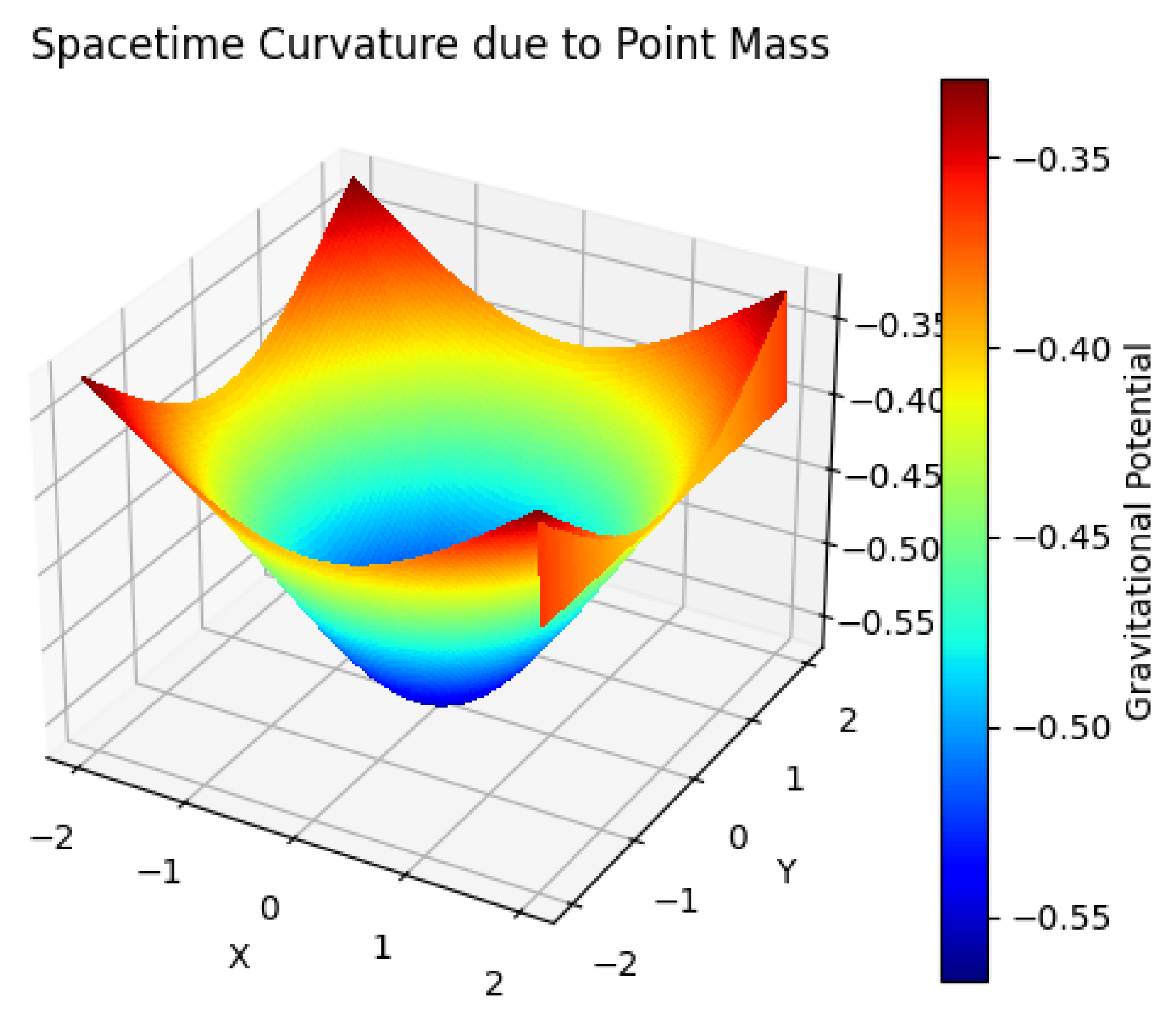
Using this, we compute the gravitational potential p in three-dimensional space:

$$p(s,x,y,z)=-{\displaystyle \frac{s}{\sqrt{x^2+y^2+z^2}}}$$

(22)

where s is the metric value at radius r. This potential is mapped over a 3D grid $x,y,z\in [-2,2]$.

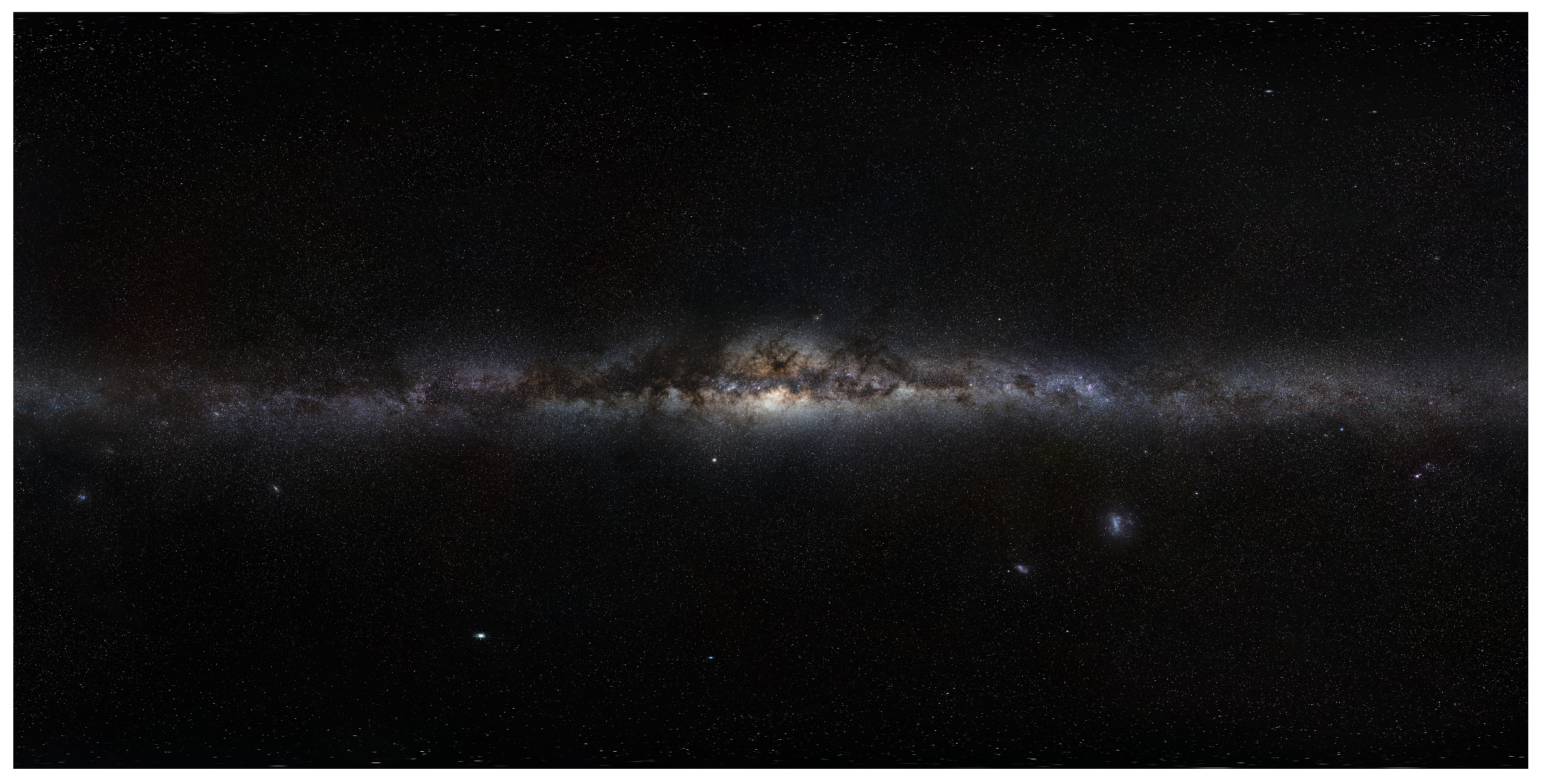
We created a simulation to add the black hole to the space. The simulation basically takes pixels of a given image, inserts black hole with a given radius and shows how would light go around the black hole following SPBP.

Here is the initial image we took.

Figure 3. Initial picture

Figure 3. Initial picture

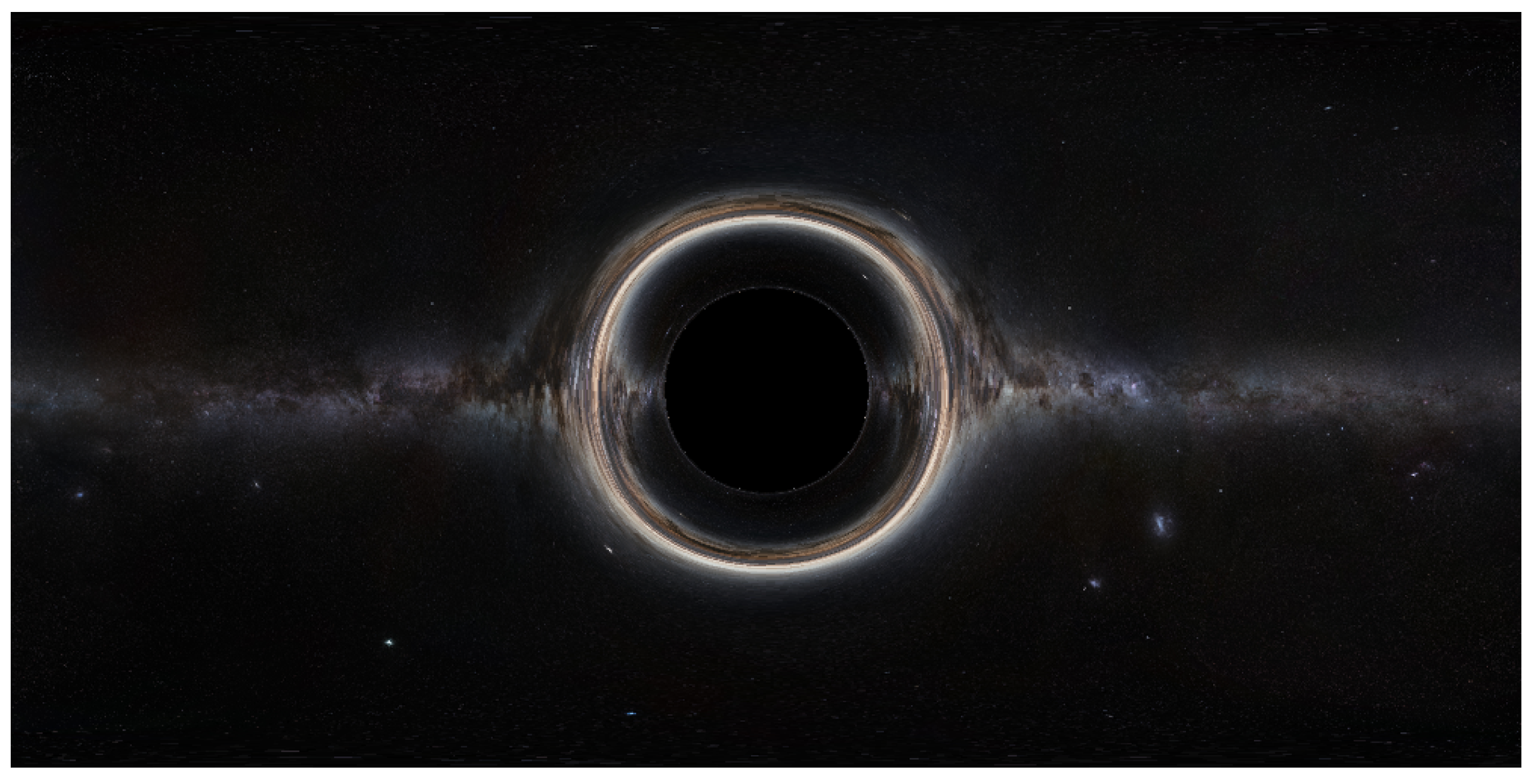
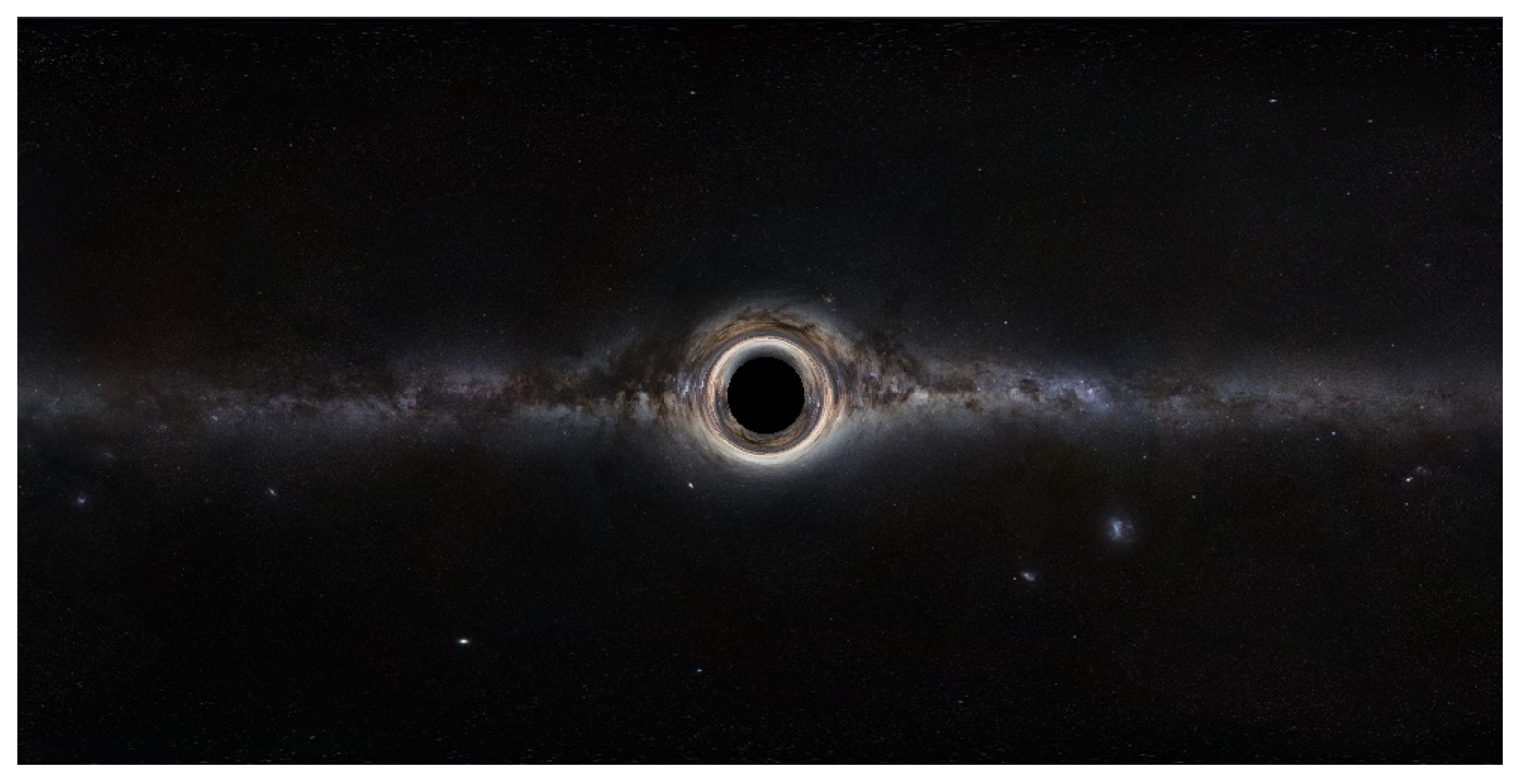
Here is the same space with the black hole inserted.

Figure 4. Picture after adding the black hole

Figure 4. Picture after adding the black hole

Here is the graph that represents the real angles of photos that escaped from black hole evolving event horizon, as well as seen angles, the angles of photons we observed which were changed due to disruption of space-time. They should be the same but they might be changed due to probabilistic nature of photons but in our theory we can predict their behavior since in is deterministic. Further we can develop a framework for quantum predictions.

Figure 5. Real angle vs Seen angle

Figure 5. Real angle vs Seen angle

Figure 6. Angles of photons movement in the entering and exiting spirals of the black hole

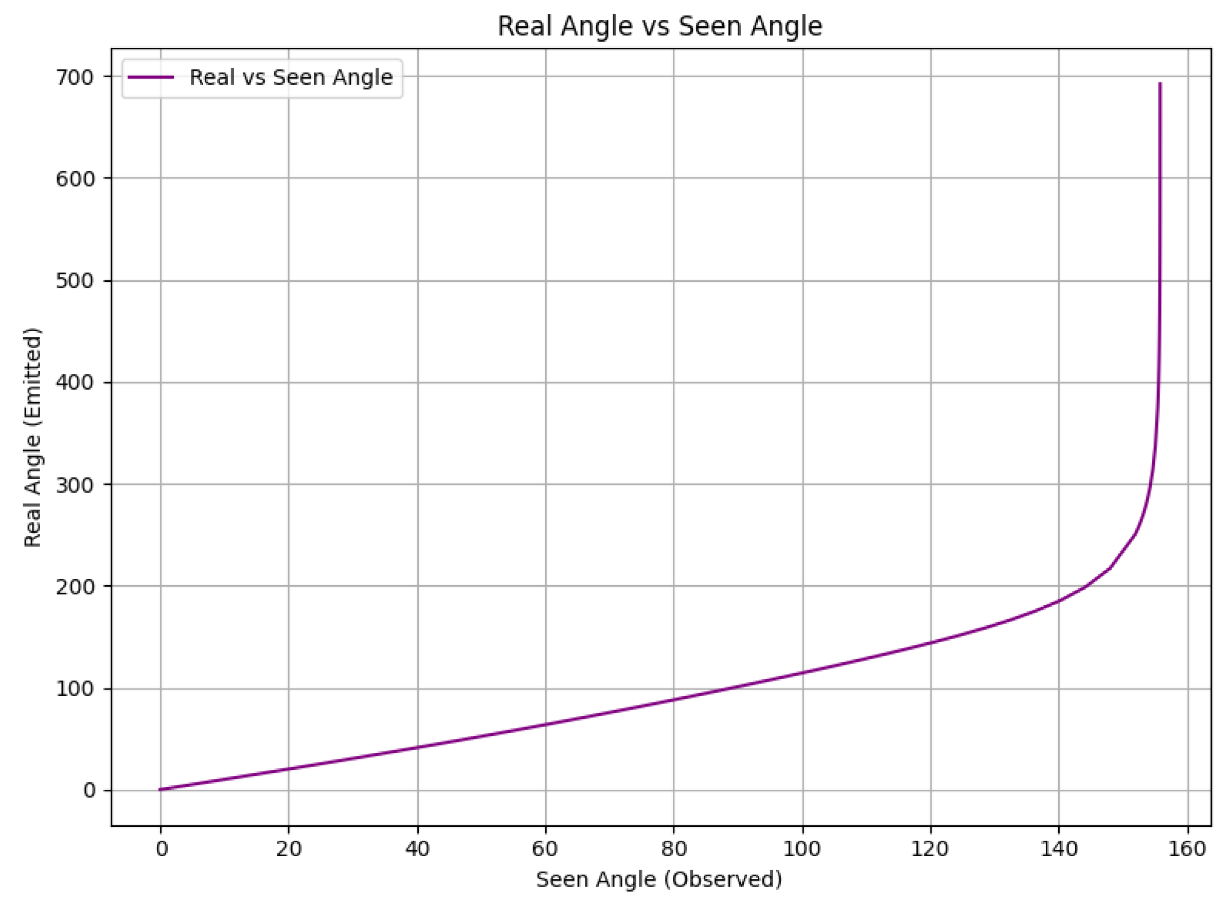
Figure 6. Angles of photons movement in the entering and exiting spirals of the black hole

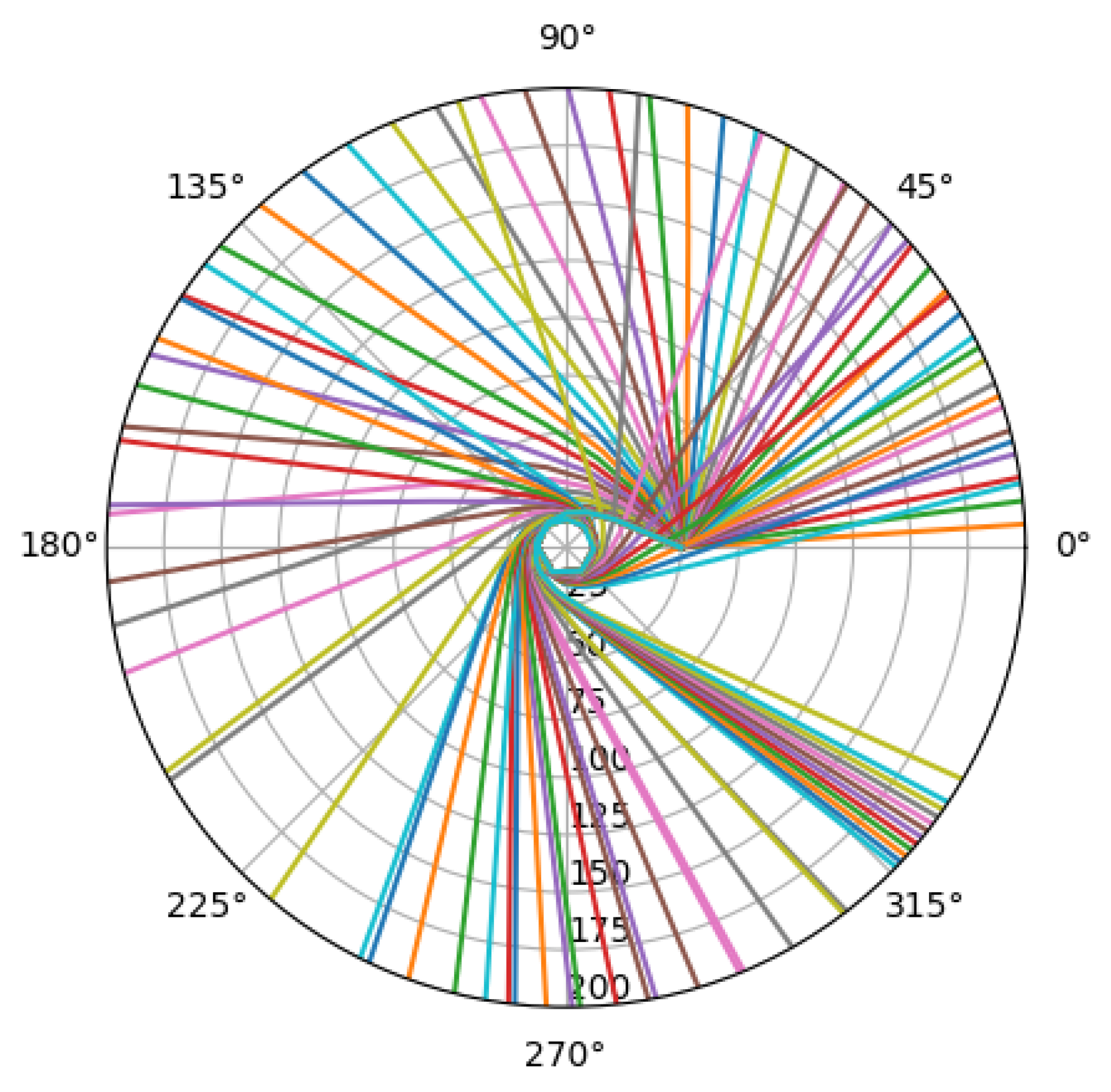
Figure 7. The other black hole insertion, with smaller radius

Figure 7. The other black hole insertion, with smaller radius

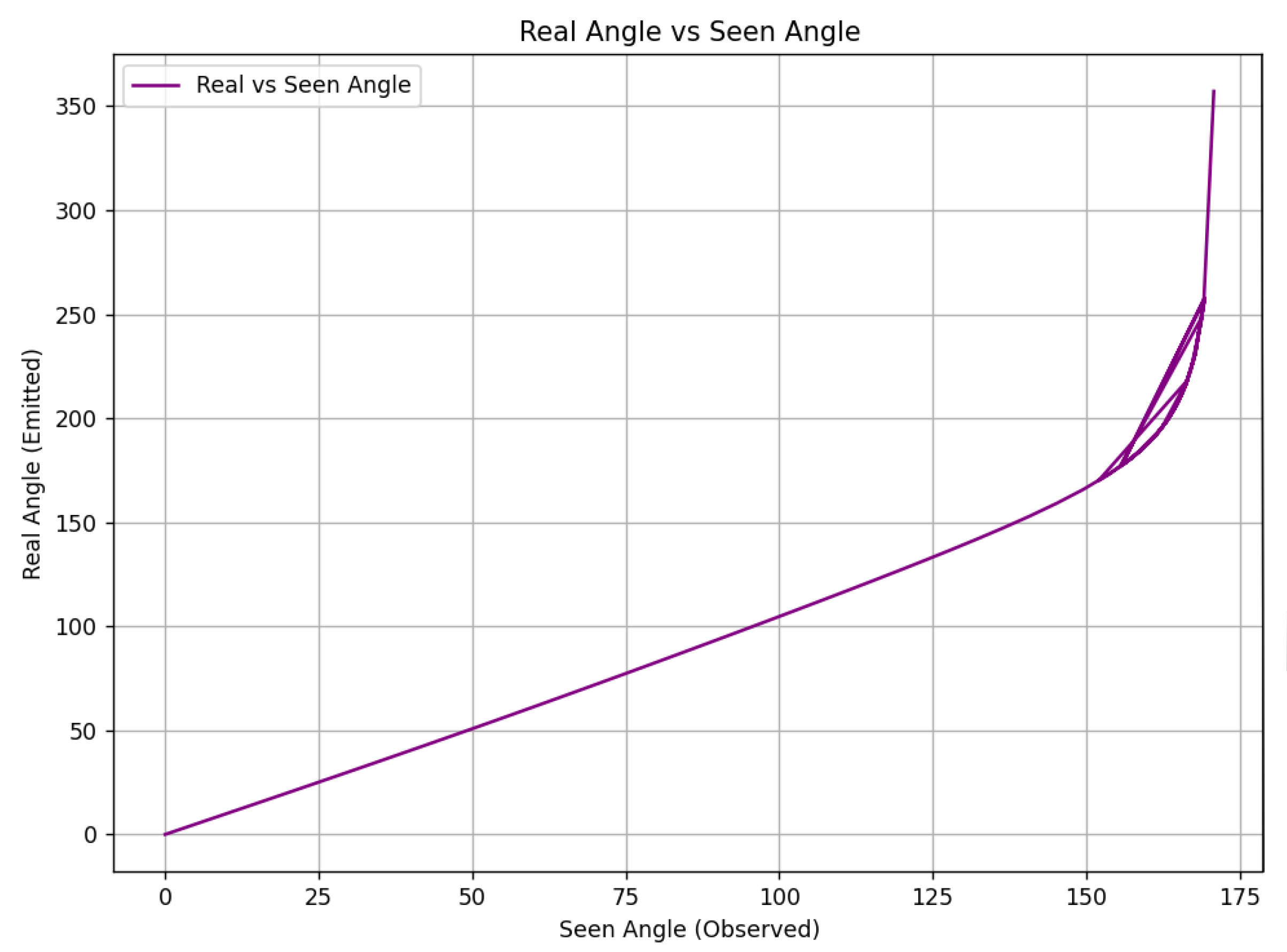
The graph illustrates the relationship between the seen angle (the observed angle of a photon’s path due to gravitational lensing) and the real angle (the actual angular trajectory taken by the photon) in the event horizon of a black hole. The non-linear distortion arises from the extreme curvature of spacetime, which is especially pronounced near the photon sphere. Traditionally, quantum mechanical behavior in such intense gravitational fields is considered probabilistic due to Planck-scale effects and the quantum uncertainty principle.

$$l_p=\sqrt{{\displaystyle \frac{\hslash G}{c^3}}}$$

However, within our deterministic reformulation of spacetime behavior near singularities, we resolve the apparent randomness and accurately predict photon trajectories. This conclusion between classical determinism and quantum uncertainty enables a clear mapping between observed and actual paths, as shown in the graph curve beyond the critical angle range.

Figure 8. Real angle vs Seen angle for the smaller black hole

Figure 8. Real angle vs Seen angle for the smaller black hole

5.1.2. Quantum Interference Near the Singularity

The classical theory breaks down as we approach the singularity. To extend our model beyond this limit, we introduce a quantum correction based on interference at a critical radius Y, where spacetime behavior transitions.

At the singularity (defined here by $r\ge Y$), we introduce a new embedding term derived from the Schrödinger equation:

$$\widehat{H}\psi =s_n^2=i\hslash {\displaystyle \frac{\partial \psi }{\partial r}}$$

(23)

Here, $\psi$ is interpreted as an integral of the metric function:

$$\psi (r)=\int s(r)dr$$

(24)

The Hamiltonian $\widehat{H}$ incorporates both thermal and gravitational potential energy. Using Hawking’s expression for black hole temperature:

$$H=T+v(r)={\displaystyle \frac{\hslash c^3}{8G\pi M{k}_b}}+v(r)$$

(25)

Substituting into the Schrödinger equation yields:

$$s_n^2=\left({\displaystyle \frac{\hslash c^3}{8G\pi M{k}_b}}+v(r)\right){\int }_0^{Y}s(r)dr=i\hslash {\displaystyle \frac{d}{dr}}\int s(r)dr=i\hslash s(r)$$

(26)

Thus, the new embedding value in the quantum-corrected region is:

$$s_n=\sqrt{s(r)i\hslash }$$

(27)

5.1.3. Interference Factor in Pre-Singularity Region

Before reaching the critical point Y, we apply an interference correction to the classical embedding value. We introduce a scaling constant $\xi$ that modulates the classical value to account for pre-singularity wave interference:

$$\xi ={\displaystyle \frac{\pi }{2}}+{\displaystyle \frac{1}{2{log}_2{(c)}^2}}$$

(28)

This constant ensures a smooth transition from classical to quantum regimes. The corrected embedding value for $r<c$ becomes:

$$s_n=\xi s(r)={\displaystyle \frac{s(r)(\pi {log}_2{(c)}^2+1)}{2{log}_2{(c)}^2}}$$

(29)

5.1.4. Unified Embedding Function

We now define the unified embedding function $s_r$ as a piecewise function:

$$s_r=\left\{\begin{array}{cc}\xi s(r)\hfill & \mathrm{if}r<c\hfill \\ \sqrt{s(r)i\hslash }\hfill & \mathrm{if}r\ge c\hfill \end{array}\right.$$

(30)

This function captures both the classical and quantum-corrected behaviors of the spacetime metric around a black hole.

5.1.5. Graphical Analysis

We visualize the corrected embedding values both in 2D and 3D:

Figure 9. Corrected embedding values in 2D

Figure 9. Corrected embedding values in 2D

Figure 10. Embedding values visualized in 3D space

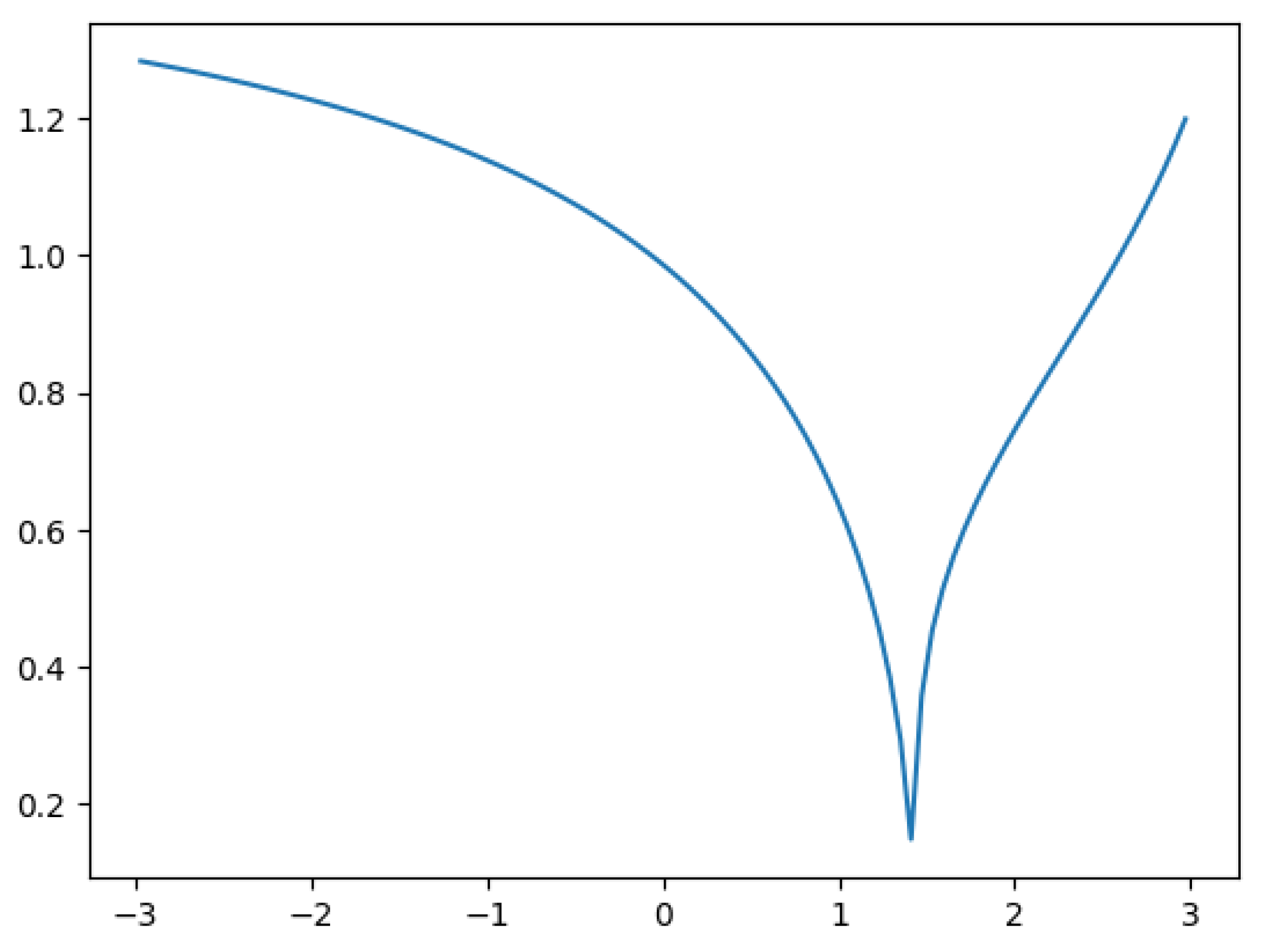
Figure 10. Embedding values visualized in 3D space

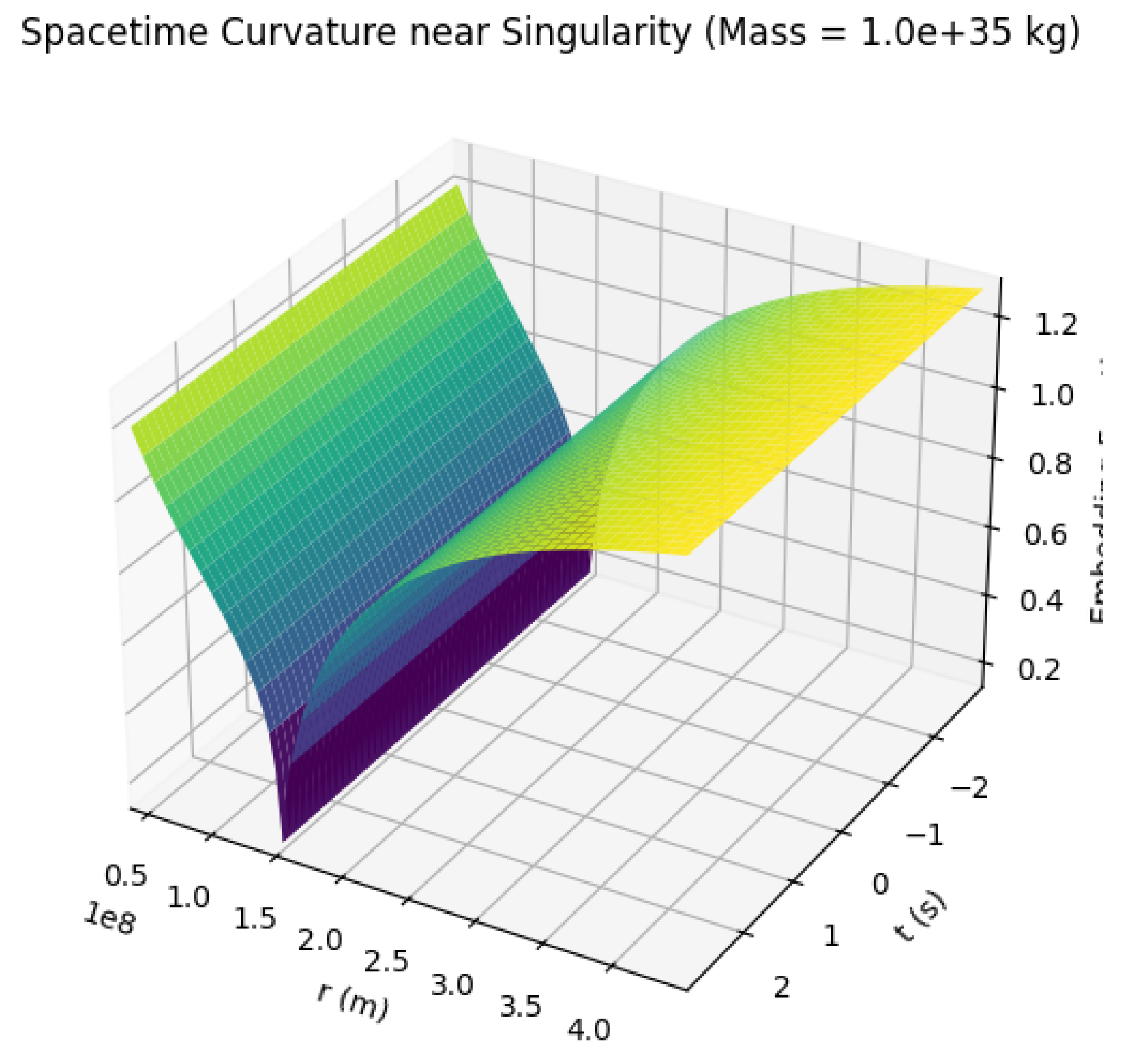
The graphs describe the space curvature in the black hole. We can visually divide each graph into 2 parts. The first part is the way towards singularity, the second is escape. The middle point is obviously singularity. So the first part is based on the increasing function and the second on the decreasing.

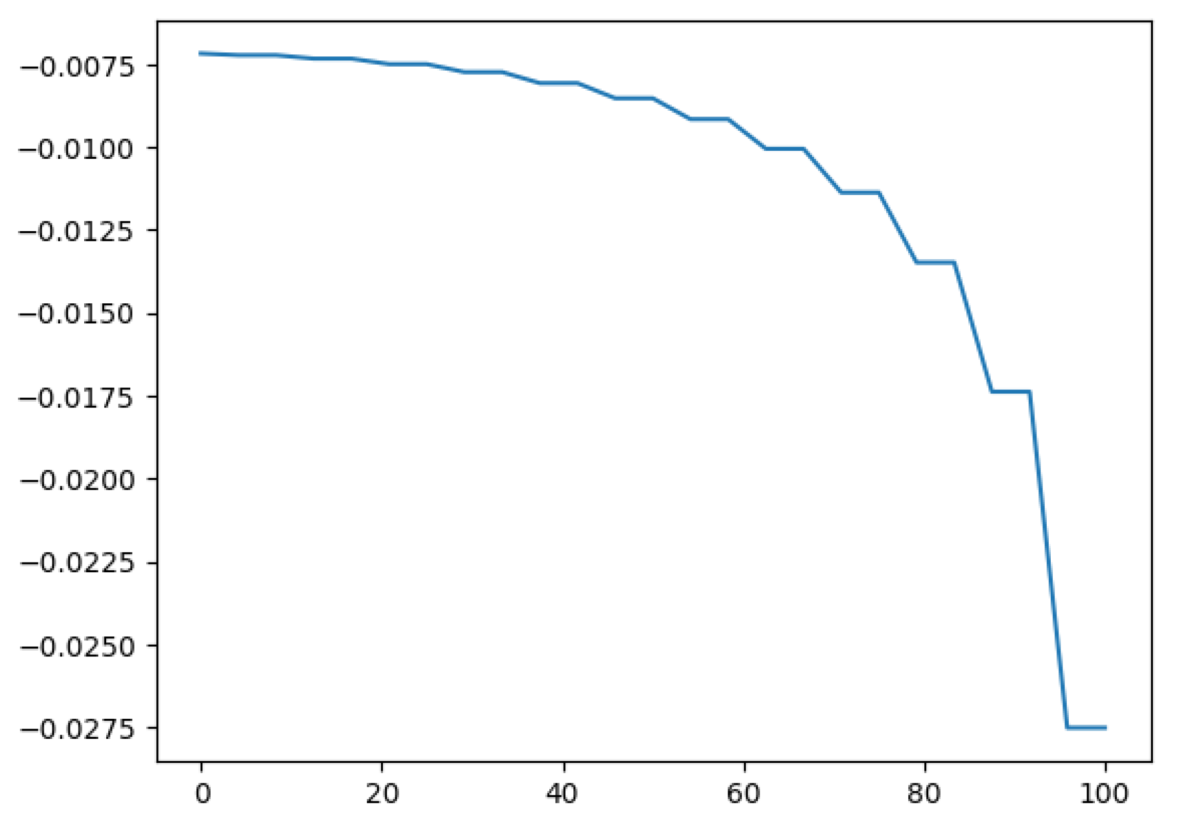
Analyzing the reverse projection in 2D, we observe a slope discontinuity and a sign change at the singularity, corresponding to the interference region:

Figure 11. Analysis of embedding transition at singularity.

Figure 11. Analysis of embedding transition at singularity.

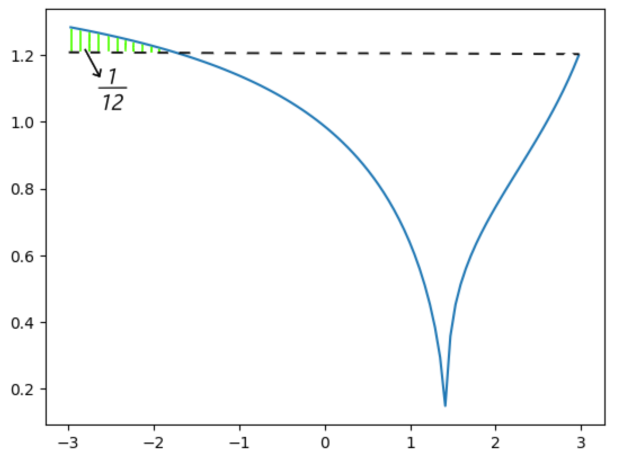
Subtracting the final embedding value from the initial value yields:

$$\Delta s=s_{\mathrm{final}}-s_{\mathrm{initial}}=-{\displaystyle \frac{1}{12}}$$

This result is consistent with our theoretical predictions and aligns with concepts from string theory and quantum gravity, indicating a finite, non-infinite behavior at the singularity. Our model suggests that spacetime collapses and transitions through the singularity via a quantum-interfered phase rather than reaching an undefined infinite state.

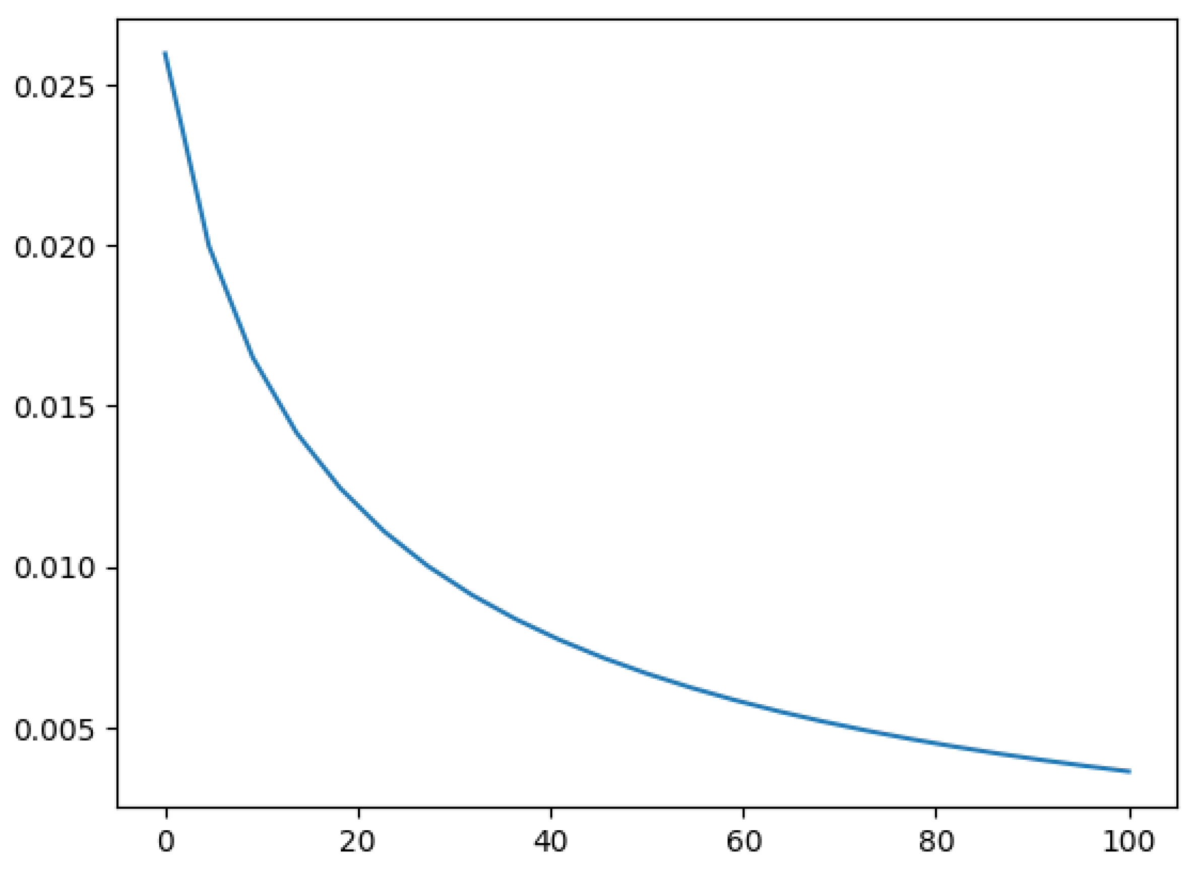
The following graph shows the pick point with the maximal mass of the black hole with. The pick point is the moment where the black hole has the biggest curvature in all its life duration. After it the black hole starts active evaporation and after some time fully evaporates.

Figure 12. The pick point of space-time curvature of a black hole

Figure 12. The pick point of space-time curvature of a black hole

Actually the other name for the pick point is Eddington Limit. The Eddington limit is when the radiation pressure force is equal to the gravitational force

$$F_{\mathrm{rad}}=F_{\mathrm{grav}}$$

Assuming electron scattering opacity,

$${\displaystyle \frac{{\sigma }_T}{c}}·{\displaystyle \frac{L}{4\pi R^2}}={\displaystyle \frac{GM{m}_p}{R^2}}$$

Therefore, the Eddington Luminosity is:

$$L_{\mathrm{Edd}}={\displaystyle \frac{4\pi GM{m}_{p}c}{{\sigma }_T}}\propto M$$

This plot presents the simulated radiation energy decay from a black hole, aligning with the theoretical predictions of Hawking radiation. The curve shows an inverse relationship between time and emitted energy, consistent with the expected thermal spectrum of black hole evaporation. In our theoretical model, deterministic formulations are used to simulate the quantum field effects near the event horizon. Despite the probabilistic nature of quantum tunneling processes, our framework reproduces the observed energy decay pattern with remarkable precision. This agreement between simulation and observation affirms the robustness of our approach and provides a bridge between quantum thermodynamics and deterministic curvature dynamics.

Figure 13. Hawking radiation

Figure 13. Hawking radiation

And here is the photo from [3] representing the observed predicted hawking radiations from a similar parameters static black hole further proving our simulation and theory.

Figure 14. Observed Hawking radiation

Figure 14. Observed Hawking radiation

Figure 15. Simulated Hawking radiation energies around a spinning black hole

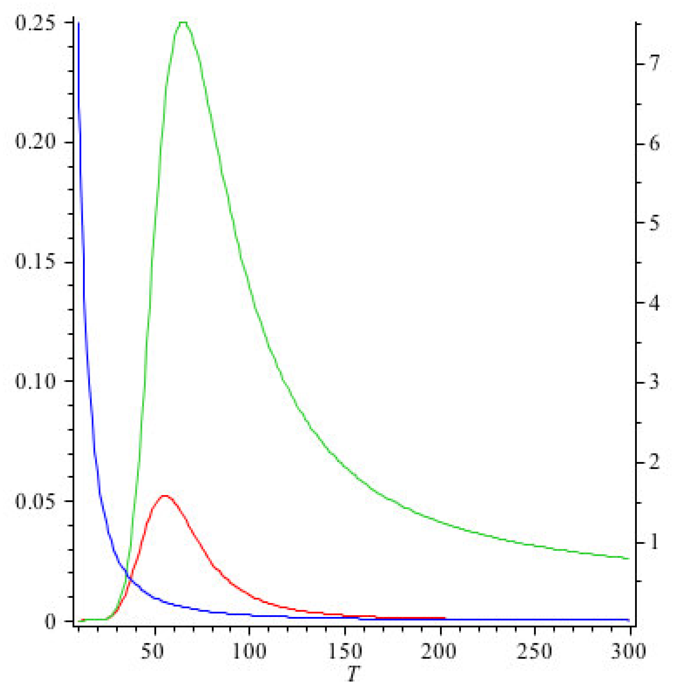
Figure 15. Simulated Hawking radiation energies around a spinning black hole

Simulated Hawking radiation energies around a spinning black hole, where is the energies is unstable due to the disturbance cause by the black hole spinning in space time which we could predict with certainty thanks to our theory.

6. Conclusions, future and ideas

6.1. Conclusions

This paper introduced a theoretical framework (Sophy-Peter Bounded Physics) as a solution to some of the most longstanding problems in modern theoretical physics, particularly the reconciliation of quantum mechanics and general relativity. At the core of this framework lies a redefinition of the foundational structure of mathematics and spacetime, where numbers are no longer linear and continuous, but instead constrained by fixed upper and lower bounds denoted as Y and E. This redefinition has a profound impact, not only mathematically but also physically, as it allows the construction of a deterministic and discrete spacetime geometry, free from the paradoxes associated with infinities.

One of the central achievements of this work is the resolution of the black hole information paradox. By capping spacetime curvature at the maximum value Y, and applying the dual behavior of increasing and decreasing functions, we demonstrated that singularities do not involve infinities but instead mark a transition point in the curvature behavior. This allows particles and information to re-emerge after entering the black hole, preventing triunity. The phenomenon of Hawking radiation, traditionally seen as probabilistic and entropic, is reinterpreted in this model as an interference-driven deterministic process emerging from the nonlinear geometric evolution near the event horizon.

Furthermore, we reformulated major physical equations, including the Schwarzschild metric, Einstein field equations, Maxwell’s equations, and the Klein-Gordon and Schrödinger equations. Each of these equations was re-expressed to incorporate bounded curvature, nonlinear derivatives, and quantum corrections. This ensures that all physical phenomena, from gravitational interactions to quantum field dynamics, remain finite and consistent.

To support these foundations, we performed numerical simulations and graphical representations of black hole geometry, photon trajectories, and quantum interference. These simulations demonstrate that light paths near black holes, which appear distorted due to classical general lensing, can be predicted under the SPBP model. Notably, the redshift, time dilation, and angle of deflection are not only quantifiable but also deterministic. Our results highlight the distinction between seen and real photon angles, confirming that classical uncertainty near singularities can be replaced with calculable, observable outcomes.

In summary, the Sophy-Peter framework provides a mathematically consistent and physically robust foundation for unifying the four fundamental forces, resolving the contradictions between quantum theory and general relativity, and reinterpreting the nature of spacetime, energy, and information. The implications of this model extend beyond theoretical physics, opening new directions in quantum physics, cosmology, and high-energy particle physics. The notion that spacetime is discrete, bounded, and inherently geometric redefines our understanding of the universe, not as a continuum governed by chance and divergence, but as a coherent, computable structure in which every outcome has a cause, every curve has a limit, and every particle follows a knowable path.

6.2. Future & Ideas

In the following scientific paper, we will talk more about determinism in quantum physics. In this paper, we already showed a couple of formulas to predict the trajectory of photon movement following the space curvature, but there is much more to tell about other particles and quantum phenomena that are currently considered non-deterministic and probabilistic. However, in SPBP, we can predict everything, and it is already partly opened in this paper. It implies that quantum physics should be redefined with deterministic formulas.

Going to the black holes, in the future, we can describe more about the spirals of particle movement or spinning nature. Also, since black holes aren’t a mystery anymore, we are able to create highly accurate simulations and get any data that interests space researchers.

There are such topics as white holes and wormholes. These concepts can be criticized or improved using our theory. In short, white holes are very unlikely to exist, while wormholes or something similar to them may be achieved using the non-linear nature of space. By curving the space to a non-linear state with a specific amount of energy, it might be possible to travel through spacetime faster than light.

References

- Sofiia Ivanko and Peter Farag, Crystal Journal of Artificial Intelligence and Applications, vol. 1, no. 1, p. 01-33, 2025.. Proof of the Riemann Hypothesis and the Modified Collatz Conjecture Using the Sophy-Peter Mathematical Framework (2025).
- Gregory Lafitte, Baeza-Yates, R., Montanari, U., Santoro, N. (eds) Foundations of Information Technology in the Era of Network and Mobile Computing. IFIP — The International Federation for Information Processing, vol 96. Springer, Boston, MA. On Randomness and Infinity. (2002).
- Donald Marolf and Henry Max eld, Department of Physics, University of California, Santa Barbara, CA 93106, USA. Observations of Hawking radiation: the Page curve and baby universes (2020).
- Panagiota Kanti and Elizabeth Winstanley, Calmet, X. (eds) Quantum Aspects of Black Holes. Fundamental Theories of Physics, vol 178. Springer, Cham.. Hawking Radiation from Higher-Dimensional Black Holes. (2015).
- Pintu Bhunia, Kallol Paul, Advances in Operator Theory, 7(1), Paper No.8, pp.1–19, “Annular bounds for the zeros of a polynomial from companion matrix” (2022).
- Leonard, Katie E. and Woodard, R. P., Phys. Rev. D 85, 104048, “Graviton corrections to Maxwell’s equations”, (2012).
- Stefan Hollands and Robert M. Wald, arXiv:1401.2026 [gr-qc], “Quantum fields in curved spacetime”, (2015).
- Bernard S. Kay, arXiv:2308.14517 [gr-qc], “Quantum Field Theory in Curved Spacetime (2nd Edition)”, (2025).
- Kugo, Taichiro and Nakayama, Ryuichi and Ohta, Nobuyoshi, Phys. Rev. D 104, 126021, “BRST quantization of general relativity in unimodular gauge and unimodular gravity”, (2021).
Disclaimer/Publisher’s Note: The statements, opinions and data contained in all publications are solely those of the individual author(s) and contributor(s) and not of MDPI and/or the editor(s). MDPI and/or the editor(s) disclaim responsibility for any injury to people or property resulting from any ideas, methods, instructions or products referred to in the content. |
© 2025 by the authors. Licensee MDPI, Basel, Switzerland. This article is an open access article distributed under the terms and conditions of the Creative Commons Attribution (CC BY) license (http://creativecommons.org/licenses/by/4.0/).
Copyright: This open access article is published under a Creative Commons CC BY 4.0 license, which permit the free download, distribution, and reuse, provided that the author and preprint are cited in any reuse.