
Submitted:
31 August 2025
Posted:
01 September 2025
You are already at the latest version
Abstract
Quasi-one-dimensional systems with multiple conduction channels are essential for describing a range of physical phenomena. In this paper, we analyse transport in wires where electrons are subject to arbitrary number of strong multi-particle backscattering terms. We present an exact calculation of the system's scattering matrix and derive a formula for the two-terminal conductance. We find the conductance is reduced from its ideal value by a term corresponding to the projection of current fields onto the subspace of integer-valued vectors characterising the gapped channels created by the perturbations. Applying this result, we establish the minimal model required to reproduce the recently observed, yet unexplained, fractional conductance plateaus with even denominators.
Keywords:
multi-channel luttinger liquids
; transport in coupled-wire systems
; fractional conductance
1. Introduction
Coupled wire models are a powerful way to model complex systems and allow the analytical methods of 1D quantum physics to be extended to higher dimensions. Starting from a Luttinger liquid model that provides a universal description of low-energy excitations in one spatial dimension [1], multiple copies can be stacked to form a discrete lattice with a continuum direction along the wire. Through coupling different wires by a multi-particle backscattering process, the highly anisotropic original geometry becomes a flexible model that can describe many different phenomena. The versatility occurs through the interactions introducing gaps into the spectrum and freezing out a sector of the field in the strong backscattering limit, resulting in controlling the number of gapped and gapless modes. This approach has proved successful for describing many different phenomena, such as the quantum Hall effect [2], fractional quantum Hall effect [3,4], topological edge modes [5,6,7], and fractons [8,9]. The transport properties of coupled wire systems, such as the two-terminal conductance in both the integer and fractional quantum Hall effect, provides an experimentally accessible way of classifying the state of the system. Therefore it is important to understand what possible values of conductance can be found from different coupled wire models.
Experimental results of the conductance in quantum point contacts with a shallow constriction [10,11] reveal conductance plateaus upon varying the depth of the constriction. The values of the conductance on these plateaus can be fractions of the quantum of conductance, , with a wide range of different fractions being found. The fractional nature of two-terminal d.c. conductance has been previously studied in two-wire systems in the presence of multi-particle backscattering [12,13,14,15]. Notably, fractions with even denominators that appear in experiment (e.g., and ) remain unexplained. In this paper we will describe the minimum possible coupled wire model that can account for these experimental conductance values.
To find these models, we introduce a rigorous way to derive the linear conductance through a generic 1D coupled wire model connected up to non-interacting leads with both forward and backward scattering interactions. This is done by starting from the `scattering’ matrix in terms of the gapped and gapless modes and carefully finding the scattering matrix in terms of the original chiral fields that describe the system far away from the interacting region. The non-local nature of the S-matrix means that the simple local rotation of fields cannot be performed directly and we must instead use the corresponding transfer matrix.
2. Model
Our system contains N coupled Luttinger liquid wires that are adiabatically connected to two non-interacting leads. Both forward scattering and multi-particle backscattering processes occur inside the interacting region . Bosonised description of this setup starts from assigning two chiral fields, and to each channel, . In terms of -dimensional vector where the N-dimensional vectors are , the Lagrangian density can be written as,
where the canonical term defines the commutation relations in the operator formulation, and the Hamiltonian, , contains forward scattering and backscattering terms,
Outside the wire (interacting section of length L) matrix tends to the diagonal matrix , where is the velocity of the i-th channel in electrodes. The contacts are assumed to be adiabatic, with the confining potential varying slowly along the wire on the scale of the Fermi wavelength for the electrons originating from the leads. This requirement results in reflectionless contacts so that any particle in the wire will transmit into the leads. The bosonic collective excitations described by a Luttinger liquid represent long-wavelength oscillations and, therefore, spatial dependences of the forward-scattering matrices inside and outside the system do not affect adiabaticity.
The n vectors , called backscattering vectors, are all integer-valued and describe the multi-particle backscattering process. For these to represent possible processes, the number of particles must be conserved in the process. Defining the `parity vector’ which is 1 for the first N entries and for the other N elements, the backscattering vectors must obey
Assuming strong backscattering limit when all , we expect that all these terms will gap the system leading to the freeze of corresponding fields, i.e., arguments of cosines. This effect is similar to locking modes in Coulomb dots [16,17] and gapped phases in the Luttinger liquid wire constraction [3]. This is possible only if the corresponding operators commute. This so-called Haldane criterion imposes that the backscattering vector satisfy
This bilinear form defines an n-dimensional vector space of backscattering vectors that satisfy this condition. In the limit of strong backscattering, which will be considered for the rest of the paper, backscattering Hamiltonian pins all sectors of the field to zero modulo . Exciting oscillations around this minimum configuration costs energy, resulting in a gap in the spectrum. Therefore it is natural to rotate the problem into a basis that distinguishes between these sectors of the field. We transform the fields via the matrix M
such that the commutation relations are unchanged. This enforces that with the group of possible transformations being the split orthogonal group . The transformation to the gapped and gapless sectors of the field can be described by the column vectors of matrix M, with the requirement that . For later calculations, it is useful to define these column vectors as,
With this transformation the arguments of cosines become . Note that this definition does not fully specify the matrix, even when there are N backscattering interactions, as there is freedom in how to define the sum of the two column vectors. This freedom in the choice of matrix M does not affect the conductance result.
2.1. Scattering And Transfer Matrices
Calculating the conductance through 1D systems requires a description of the contacts and external leads. In both the original quantisation of conductance for a non-interacting system [18] and when there is a region of forward scattering [19,20,21,22], the leads solely determine the d.c. conductance. The dominance of the leads suggests that we can consider the transport problem with a scattering matrix that connects the incoming and outgoing original chiral fields, and . These fields propagate freely outside the interacting section of the wire but are mixed up inside the wire. However, when incoming excitations are in the energy gap, all the gapped sectors of the field will not be supported inside the wire and must be reflected in the low temperature limit. Therefore, there will be a simple description of the `scattering’ matrix in terms of the gapped and gapless modes. The gapped and gapless modes are not guaranteed to be chiral, so they are not related simply to incoming and outgoing modes, but the equivalent ’scattering’ matrix still relates the values of the fields on either side of the interacting region.
The crux of the problem is that our knowledge of the sectors of fields is for local linear combinations of the original chiral fields, but the S-matrix is a non-local object. In order to change the local basis of the S-matrix we first must create the appropriate transfer matrix. Then the local transformation of fields can be applied, and the corresponding scattering matrix in terms of the original chiral fields can be found. An important point to note is that transfer matrices cannot be meaningfully defined when there is perfect reflection, so the limit of perfect reflection can only be taken for the S-matrix.
Figure 1.
Demonstrating how to relate scattering matrices in different bases through implementing the local rotation of fields on the transfer matrices, which are local objects. The S matrix relating combinations of fields at can be determined easily in the gapped and gapless basis but this is a non local object, while the transfer matrix acts on local combinations of fields.
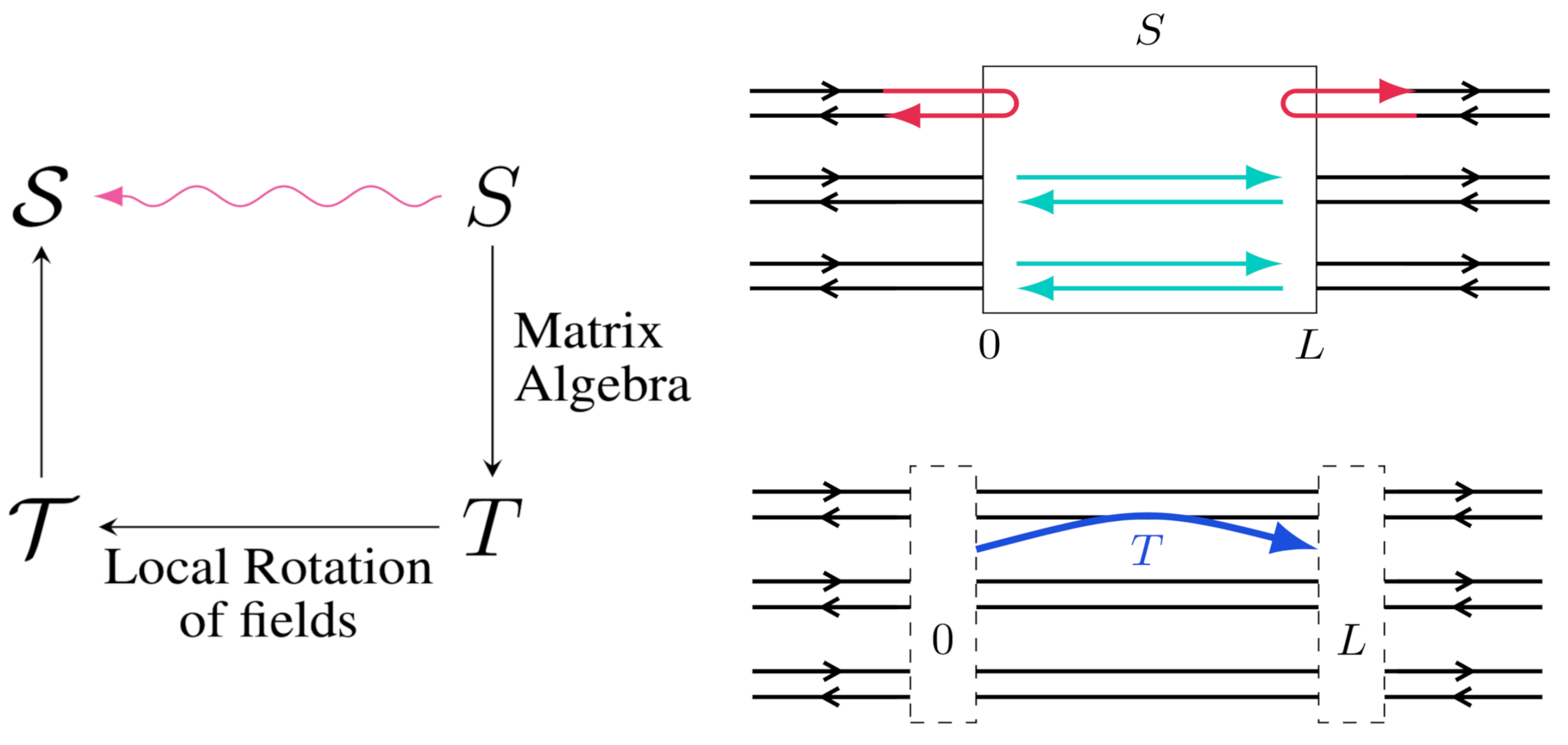
The scattering matrix and the transfer matrix are defined by a combination of the original chiral fields at two points ,
The two matrices can be related to each other through matrix algebra,
where are matrices that connect the right and left movers at different positions . The transfer matrix for the rotated fields T can be found by applying the transformation M
which defines the relation between the transfer matrices . Finally we can get the S-matrix in the rotated basis through inverting Equation (8). In this basis, for energies below the size of the gap at low temperatures and small voltages, the gapped sectors will fully reflect, and the gapless sectors will perfectly transmit. However, as mentioned earlier, due to the divergence of the transfer matrices, we cannot assume that the S-matrix perfectly reflects, and therefore we must consider the more general case and take the perfect reflection limit at the end.
To illustrate the process, we start with the one-channel case. In the rotated fields, we can write the scattering matrix as
with current conservation, giving the conditions . We only consider the situation of complete reflection and perfect transmission , which means that we can consider and . The corresponding transfer matrix in this basis can be expressed using
Although the perfect transmission limit is well defined as , the limit diverges. This can be understood as a transfer matrix that gets reflected, will not relate the fields on either side of the wire, resulting in a singular matrix.
Performing any local rotation of chiral fields on the transfer matrix and then finding the equivalent scattering matrix for the rotated fields will result in the limit producing a finite matrix with only non-zero off-diagonal elements. Upon implementing current conservation, the off-diagonal elements will be equal to one and match Equation (10). In the one-channel case, this states something obvious, that any linear combinations of chiral fields on either side of the interacting section are completely unrelated to each other in the case of perfect reflection. This freedom of choice in rotation of the chiral fields is a product of the limit and will manifest again when we include more channels into the description.
For multiple channels, the scattering matrix will be given by
where are all matrices with entries and these describe the reflection and transmission of each channel. Current conservation now becomes the expression , but if we assume that there is no scattering between channels, then we will have current conservation in each channel so that . Then the total transfer matrix can be written as
where is the reflection ratio for each channel. For any of the that correspond to gapless modes, these can be safely taken to be 0 as the transfer matrices are well defined. The remaining , where a now only indexes the gapped sectors, can be set to the same value as they will all be taken to be infinite. This allows us to simplify the transfer matrix to be where repeated indices now imply summation. Using the transformation in Equation (9) we can find the transfer matrix in the original fields, for where are N-dimensional vectors,
The matrix can be explicitly inverted to give
where with the equality guaranteed from the Haldane criterion in Equation (4). The matrix refers to the -th element of the inverse of matrix . Therefore, the scattering matrix in the new basis will be
which defines the transmission and reflection elements in the original basis. In the total reflection limit, we can see that , which then means that the operators become projectors.
= 1mathvariantdouble-struck2N - 2ΠG for being the projector onto the space G.
The d.c. current through the system can be written in terms of the scattering matrix by symmetrising the current on either side of the scattering region. Using the ’parity’ vector of Equation (3), the total d.c. current is defined as,
To show that these two expressions are equivalent, subtract the two vectors and use the particle conservation requirement. This equality implies that the total current is constant across the system. This then allows the total current to be written as a symmetrisation of the previous equation
where . The incoming currents are emitted from the reservoirs at chemical potentials for the left and right reservoirs, respectively. The voltage drop across the system will be the difference between the chemical potentials and therefore the conductance is given by
All of the details of the forward scattering interactions drop out in the d.c. limit and the conductance is entirely determined by the space created by the backscattering vectors. Note that this can be represented as projecting to the orthogonal complement space to G. This space can be decomposed into two orthogonal spaces and F, where and the free space is what remains, . From Equation (4), we can see that the spaces G and are orthogonal. Therefore the projector can be written as . However, due to the structure of vectors , as they must satisfy due to current conservation, the projector does not contribute to the conductance in Equation (21). The conductance can then be written as , the overlap of the parity vector with the projection of the parity vector on the free space.
3. Results
To show the complementary approach of calculating the gapped and free projection operators, we will consider two cases in the N wire system - one backscattering interaction and backscattering interactions.
3.1. Single Backscattering Mechanism
When only one backscattering vector is relevant, the projection operator can be simply constructed. The interaction can encompass multiple wires, but the corresponding vector must satisfy Equation (3) and (4). An illustration of a possible realisation of this is shown in Figure 2 where l particles scattering from the left to right movers in one channel is balanced by m and n particles scattering in the opposite direction in two other channels.
We can construct the projection operator onto a vector using . The total conductance through the system becomes,
3.2. Single Gapless Mode
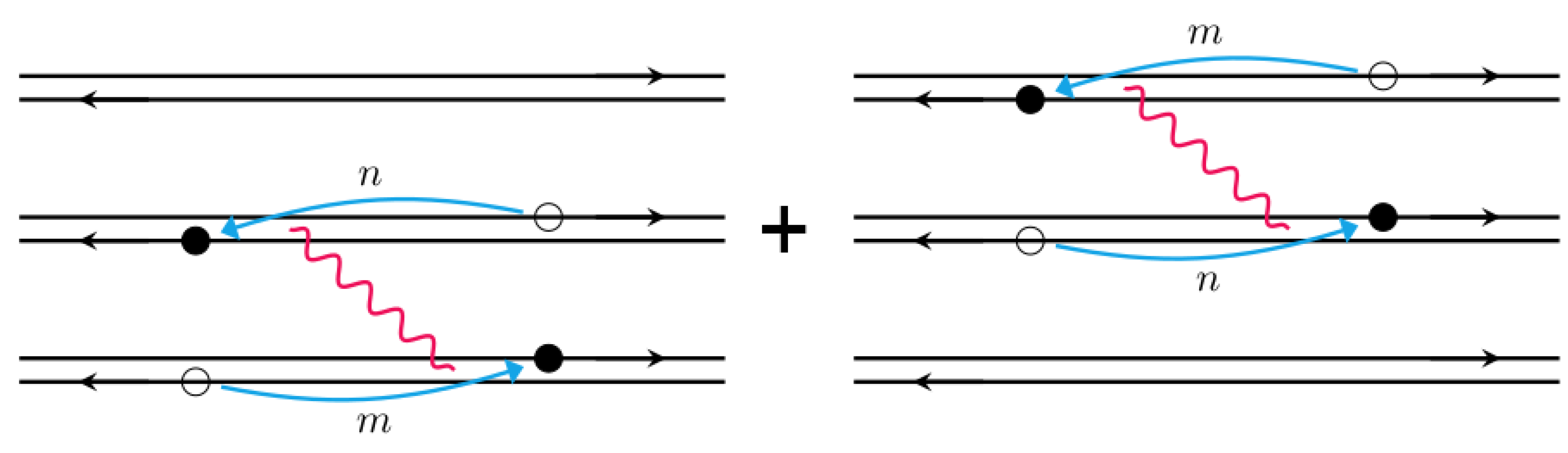
To show how to utilise the free sector description, we now consider an N-channel system with identical interactions between all neighbouring wires described by -dimensional backscattering vectors [2,23]. The interaction between the first two wires is . All other interaction vectors are obtained by a shifting non-zero values of , consequently to the right. An example of such a system with three channels is shown in Figure 4.
There are two ways to approach the construction of the projector in the gapped space. One possibility is to explicitly construct from all n perturbation vectors by putting them as column vectors into the matrix and calculating (one should keep in mind that is a matrix and not a square one). Another option is to construct an orthonormal basis for the space . Then the projection can be written as . However, from Equation (20) we can construct the orthogonal projection onto the free space by finding vectors that are orthogonal to all and . Calling ,
The other vector in the free space is given by , but it does not contribute to the conductance as . Therefore, we can write the projector onto the free space as . Then, using equation , we find the conductance
in a perfect agreement with the case considered in Reference [23], and the result for the two-wire system obtained above in Equation 22. When the number of channels , then the result becomes
4. Finding Even Denominators
Having applied the conductance equation to specific backscattering interactions, we can now ask the inverse question of what backscattering interaction can produce a specific value of conductance. The most puzzling results of the experiments [10] are the fractional conductances with even denominators. For a two-channel system with only one relevant perturbation, Equation (22), there can only be conductance with odd denominators. The proof of this can be seen through choosing both to have the same parity (in order to guarantee that the denominator is even), with the even parity case being insensitive to an overall factor of 2 and the odd parity case having an odd denominator. Through this, any choice of even can be reduced into the case of opposite parity or odd covering all possibilities. A similar, but lengthier, procedure of mathematical induction shows that conductances of systems with three and four channels can also have only odd denominators.
The smallest number of channels, and therefore the minimal coupled wire model, necessary for an even denominator in the presence of one relevant perturbation is five (). Surprisingly, choosing the perturbation that involves the smallest nontrivial number of quasiparticles in all five channels provides the conductance
To discuss possible values of conductance in systems with many channels in the presence of n relevant perturbations, it is easiest to first consider the case where all backscattering vectors , where , are orthogonal to each other. Using the Haldane criterion and particle conservation, the conductance can be written in terms of only N-dimensional vectors ,
This simplified expression shows how the total conductance is the difference between the number of channels (which is the conductance of the system in the absence of perturbations) and the conductance “stolen” by the gapped channels. To have g be an even denominator fraction, at least one of the terms in the a sum must be a fraction with an even denominator; therefore, we can restrict our attention to terms with this form.
According to the experiments, the wires have spinful channels due to the lack of an external magnetic field, and therefore, a coupled wire model that describes the appearance of even denominator fractions must have an even number of channels. For the wire system, both the and conductance fractions can be obtained with orthogonal backscattering interactions. The two perturbations and lead to
With the addition of another orthogonal perturbation, , we can find
Very recent experiments have shown a fractional conductance plateau of [24] and the minimal coupled wire model needed to obtain this result exactly has channels with three mutually orthogonal perturbations.
Although we have only discussed the case when all the backscattering vectors are orthogonal, this analysis holds when the vectors are linearly independent. For any non-colinear vectors, we can construct orthogonal vectors through Gram-Schmidt and choose a scaling of the new orthogonal vector such that every element has integer values. The projection operator is independent of a basis chosen to span the space G and therefore the conductance for any backscattering operators can be represented by Equation (27) with the appropriate choice of .
5. Discussion
In constructing the minimal coupled wire model required to match experimental measurements of fractional conductance plateaux, we have made no attempt to provide a microscopic reasoning for the occurrence of the backscattering interactions. It is important to note that there are multiple different choices of backscattering operators that can produce the same conductance result due to the projection operator that appears in the conductance. However, they will differ by the number of particles involved in the multi-particle backscattering, with higher-order processes becoming increasingly unlikely. The fact that at least 6 (three spin-degenerate) channels are required to get an even denominator fractional conductance, with more channels for higher multiples of 2 in the denominator, means that any coupled wire model must explain the appearance of extra channels.
Finally, it is possible to approach even-denominator fractions using results with odd denominators. The difference between the approximation and the actual value comes at the expense of higher-order multi-particle backscattering. For example, in the four-channel case with three two-wire perturbations, where we can use Equation (24), if by then the conductance is . Choosing instead produces a closer result of , but requires more particles to be involved in the backscattering, resulting in the process being less likely to be relevant.
Future work is to examine more transport characteristics of these systems, such as shot noise, in order to determine the nature of the quasiparticles in the gapped sector.
Author Contributions
All authors equally contributed to all aspects of this research and preparation of the manuscript.
Funding
This work was supported by the SCE internal grant EXR01/Y17/T1/D3/Yr1 (V.K.). IVY gratefully acknowledges support from the Leverhulme Trust under the grant RPG-2024-124
Acknowledgments
The authors (V.K. and I.V.Y.) are grateful for the hospitality extended to them at the Center for Theoretical Physics of Complex Systems, Daejeon, South Korea, and at the Max-Planck-Institut für Physik Komplexer Systeme, Dresden, Germany, where this research had started. The authors are grateful to M. Pepper for illuminating discussions. R.D. would like to thank A. Walker for discussions.
Conflicts of Interest
The authors declare no conflicts of interest.
References
- Haldane, F.D.M. Luttinger liquid theory of one-dimensional quantum fluids. I. Properties of the Luttinger model and their extension to the general 1D interacting spinless Fermi gas. Journal of Physics C: Solid State Physics 1981, 14, 2585–2609. [Google Scholar] [CrossRef]
- Kane, C.L.; Mukhopadhyay, R.; Lubensky, T.C. Fractional Quantum Hall Effect in an Array of Quantum Wires. Phys. Rev. Lett. 2002, 88, 036401. [Google Scholar] [CrossRef] [PubMed]
- Teo, J.C.Y.; Kane, C.L. From Luttinger liquid to non-Abelian quantum Hall states. Phys. Rev. B 2014, 89, 085101. [Google Scholar] [CrossRef]
- Fuji, Y.; Furusaki, A. Quantum Hall hierarchy from coupled wires. Phys. Rev. B 2019, 99, 035130. [Google Scholar] [CrossRef]
- Meng, T.; Neupert, T.; Greiter, M.; Thomale, R. Coupled-wire construction of chiral spin liquids. Phys. Rev. B 2015, 91, 241106. [Google Scholar] [CrossRef]
- Kagalovsky, V.; Chudnovskiy, A.L.; Yurkevich, I.V. Stability of a topological insulator: Interactions, disorder, and parity of Kramers doublets. Phys. Rev. B 2018, 97, 241116. [Google Scholar] [CrossRef]
- Yurkevich, I.; Kagalovsky, V. Superconducting edge states in a topological insulator. Scientific Reports 2021, 11, 18400. [Google Scholar] [CrossRef]
- Sullivan, J.; Dua, A.; Cheng, M. Fractonic topological phases from coupled wires. Phys. Rev. Res. 2021, 3, 023123. [Google Scholar] [CrossRef]
- Fuji, Y.; Furusaki, A. Bridging three-dimensional coupled-wire models and cellular topological states: Solvable models for topological and fracton orders. Phys. Rev. Res. 2023, 5, 043108. [Google Scholar] [CrossRef]
- Kumar, S.; Pepper, M.; et al. Zero-Magnetic Field Fractional Quantum States. Phys. Rev. Lett. 2019, 122, 086803. [Google Scholar] [CrossRef] [PubMed]
- Kumar, S.; Pepper, M. Interactions and non-magnetic fractional quantization in one-dimension. Appl. Phys. Lett. 2021, 119, 110502. [Google Scholar] [CrossRef]
- Meng, T.; Fritz, L.; Schuricht, D.; Loss, D. Low-energy properties of fractional helical Luttinger liquids. Phys. Rev. B 2014, 89, 045111. [Google Scholar] [CrossRef]
- Aseev, P.P.; Loss, D.; Klinovaja, J. Conductance of fractional Luttinger liquids at finite temperatures. Phys. Rev. B 2018, 98, 045416. [Google Scholar] [CrossRef]
- Cornfeld, E.; Neder, I.; Sela, E. Fractional shot noise in partially gapped Tomonaga-Luttinger liquids. Phys. Rev. B 2015, 91, 115427. [Google Scholar] [CrossRef]
- Shavit, G.; Oreg, Y. Fractional Conductance in Strongly Interacting 1D Systems. Phys. Rev. Lett. 2019, 123, 036803. [Google Scholar] [CrossRef] [PubMed]
- Sedlmayr, N.; Yurkevich, I.V.; Lerner, I.V. Tunnelling density of states at Coulomb-blockade peaks. Europhysics Letters 2006, 76, 109. [Google Scholar] [CrossRef]
- Yurkevich, I.V.; Lerner, I.V. Nonlinear σ model for disordered superconductors. Phys. Rev. B 2001, 63, 064522. [Google Scholar] [CrossRef]
- Lesovik, R.; Glazman, L.; Khmelnitskii, D.; Shekhter, R. Reflectionless quantum transport and fundamental ballistic-resistance steps in microscopic constrictions. Jetp Letters 1988, 48, 238–241. [Google Scholar]
- Maslov, D.L.; Stone, M. Landauer conductance of Luttinger liquids with leads. Phys. Rev. B 1995, 52, R5539–R5542. [Google Scholar] [CrossRef] [PubMed]
- Safi, I.; Schulz, H.J. Transport in an inhomogeneous interacting one-dimensional system. Phys. Rev. B 1995, 52, R17040–R17043. [Google Scholar] [CrossRef] [PubMed]
- Ponomarenko, V.V. Renormalization of the one-dimensional conductance in the Luttinger-liquid model. Phys. Rev. B 1995, 52, R8666–R8667. [Google Scholar] [CrossRef] [PubMed]
- Egger, R.; Grabert, H. Applying voltage sources to a Luttinger liquid with arbitrary transmission. Phys. Rev. B 1998, 58, 10761–10768. [Google Scholar] [CrossRef]
- Oreg, Y.; Sela, E.; Stern, A. Fractional helical liquids in quantum wires. Phys. Rev. B 2014, 89, 115402. [Google Scholar] [CrossRef]
- Liu, L.; Gul, Y.; Holmes, S.; Chen, C.; Farrer, I.; Ritchie, D.; Pepper, M. Possible zero-magnetic field fractional quantization in In0. 75Ga0. 25As heterostructures. Applied Physics Letters 2023, 123. [Google Scholar] [CrossRef]
Figure 2.
Depicting a possible backscattering interaction that results in one sector of the fields being pinned to zero. The empty holes indicate an annihilation operator has acted on that chiral field, and the filled circles correspond to particles being created. This would be described by .
Figure 2.
Depicting a possible backscattering interaction that results in one sector of the fields being pinned to zero. The empty holes indicate an annihilation operator has acted on that chiral field, and the filled circles correspond to particles being created. This would be described by .
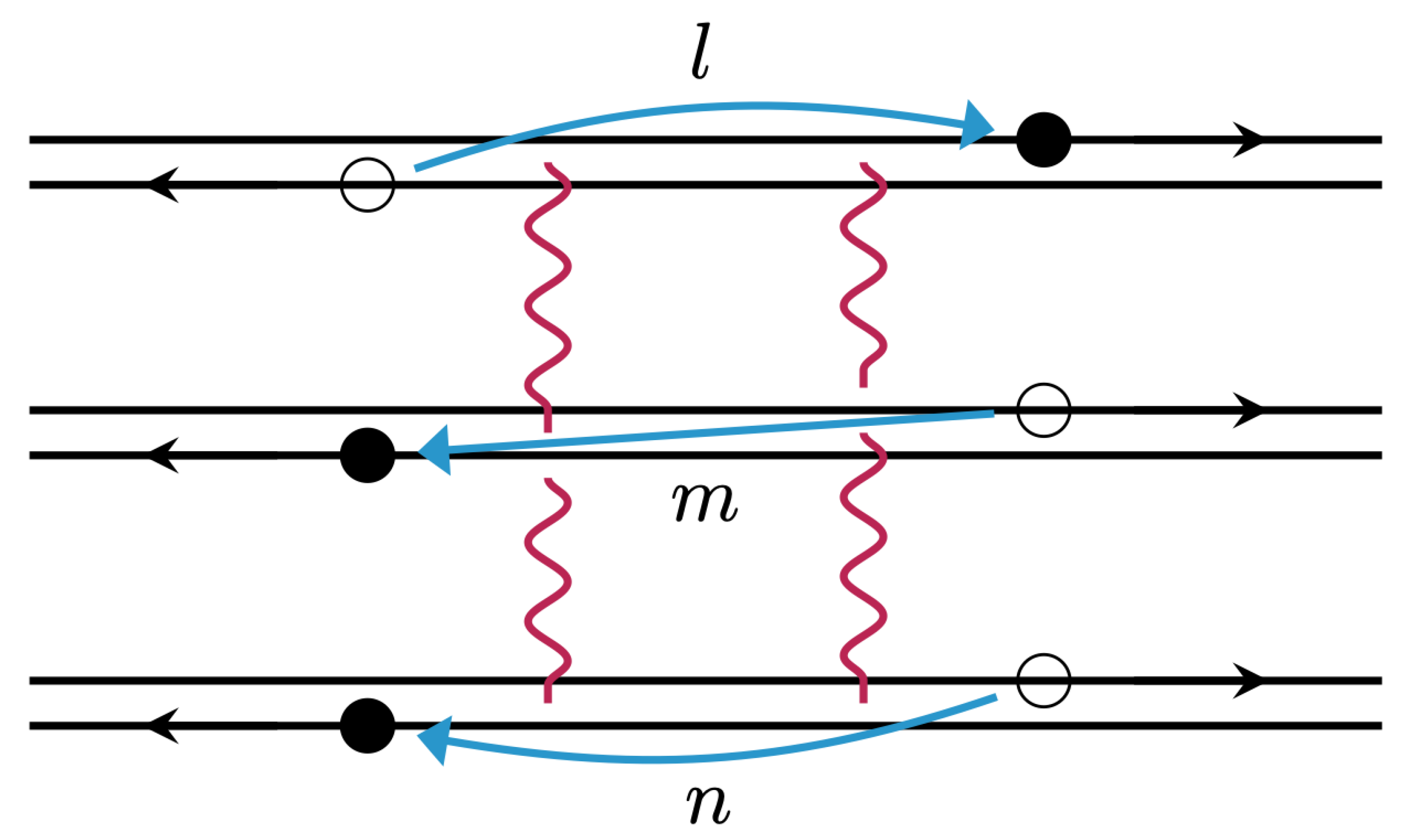
Figure 3.
The possible different fractions that can be obtained from the two-wire case. a) The surface produced by Equation (22). Notably the conductance is always zero for and equal to two for . b) The fractional conductance values are show for integer values of for two different lines along the surface. The upper plot shows the values when , as originally discussed in Reference [23], while the lower plot is for .
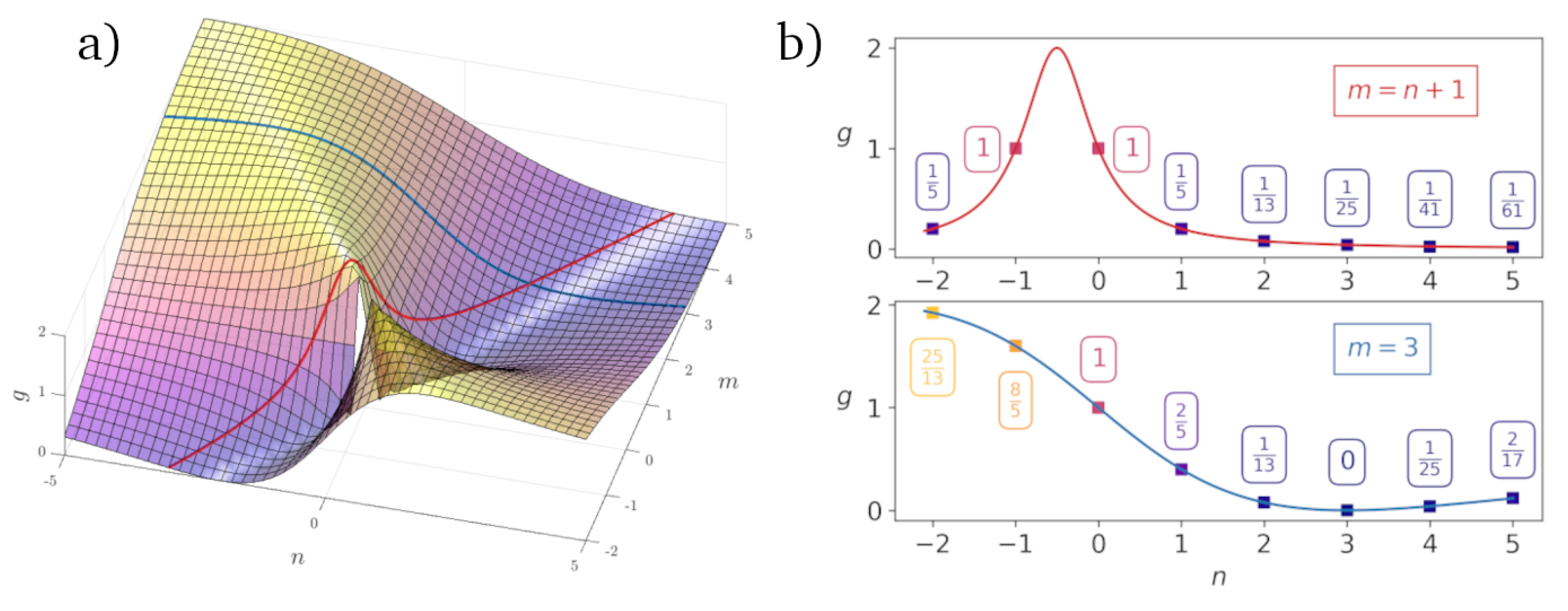
Figure 4.
Constructing a single gapless mode from two 2-wire interactions in a 3 wire system. This backscattering would be described by the vectors .
Figure 4.
Constructing a single gapless mode from two 2-wire interactions in a 3 wire system. This backscattering would be described by the vectors .
Disclaimer/Publisher’s Note: The statements, opinions and data contained in all publications are solely those of the individual author(s) and contributor(s) and not of MDPI and/or the editor(s). MDPI and/or the editor(s) disclaim responsibility for any injury to people or property resulting from any ideas, methods, instructions or products referred to in the content. |
© 2025 by the authors. Licensee MDPI, Basel, Switzerland. This article is an open access article distributed under the terms and conditions of the Creative Commons Attribution (CC BY) license (http://creativecommons.org/licenses/by/4.0/).
Copyright: This open access article is published under a Creative Commons CC BY 4.0 license, which permit the free download, distribution, and reuse, provided that the author and preprint are cited in any reuse.


