
Submitted:
28 August 2025
Posted:
01 September 2025
You are already at the latest version
Abstract
Pedestrian crashes remain a leading cause of road traffic fatalities in developing coun-tries (DCs), yet reliable crash data are scarce, limiting the calibration of global safety models such as the International Road Assessment Programme (iRAP) to local contexts. This study presents a methodological framework for quantifying the influence of con-textual risk factors on pedestrian crash frequency in data-scarce environments. Artificial datasets comprising 2000 random samples per variable were generated from litera-ture-derived distributions representing DC conditions. Analytical procedures, includ-ing pairwise correlation, stepwise regression, and Negative Binomial (NB) modelling, were applied to estimate Factor Influence values (Fi) and identify variables absent from the iRAP model. Six NB models were developed; none of the 20 modelled variables met conventional statistical significance thresholds, underscoring that the results are illus-trative rather than inferential. Comparative analysis revealed 16 factors absent from iRAP, including “countermeasure as an afterthought” (Fi = 0.63), and 5 factors neither modelled nor covered by iRAP. This approach demonstrates a replicable process for prioritising safety factors in DC contexts, to be calibrated with real-world data in future studies.
Keywords:
pedestrian safety
; contextual risk factors
; artificial data
; negative binomial model
; data-scarce environments
; iRAP
; developing countries
1. Introduction
Pedestrian safety remains a pressing challenge in developing countries (DCs), where pedestrians account for a disproportionately high share of road traffic fatalities [1]. Existing safety assessment frameworks, such as the International Road Assessment Programme (iRAP), rely on countermeasure effectiveness values derived largely from high-income country (HIC) data [2]. While robust in well-documented contexts, such models may misrepresent actual risk dynamics in DCs due to fundamental differences in traffic operations, enforcement, infrastructure quality, and road user behaviour [3,4].
Accurate modelling of pedestrian crash risk in DCs is hindered by sparse and often unreliable crash data, with underreporting rates as high as 84% in some regions [5]. Traditional statistical modelling therefore faces limitations in these contexts, necessitating innovative approaches that leverage available literature, expert knowledge, and proxy datasets [6]. To address this challenge, the authors recently conducted a systematic literature review (SLR), which identified 33 contextual factors that influence the effectiveness of pedestrian safety countermeasures in DCs. These factors were categorised into four groups: traffic exposures and operational characteristics, land use and planning, demographics, and infrastructure and roadway characteristics [7,8]. This body of evidence provides a basis for developing methodological frameworks that can function in data-scarce environments.
The present study builds upon the findings of this SLR and has two primary objectives. First, to quantify the relative influence of contextual factors on pedestrian crash outcomes by generating artificial datasets informed by literature-derived distributions and applying correlation analysis, regression modelling, and regression coefficient transformations to derive risk factor influence values (Fi). Second, to compare these regression transformation results against the iRAP framework, thereby identifying important contextual factors that may not be adequately reflected in existing predictive tools.
It is important to emphasise that this study does not seek to provide empirically generalisable estimates of risk factor influence values (Fi). Rather, it presents an illustrative methodological process that can be replicated and calibrated when reliable crash data become available in DCs. To this end, the study follows a structured approach:
- Extracting trend data of contextual factors from literature sources.
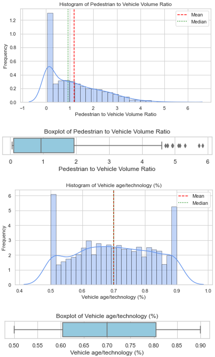
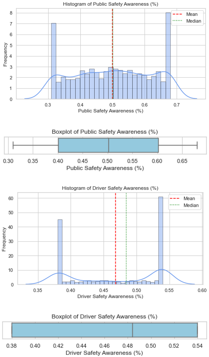
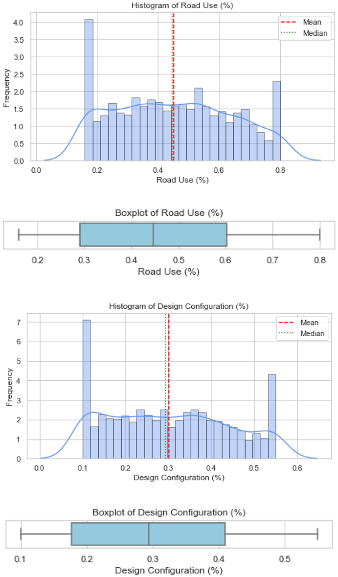
- Generating a representative artificial dataset based on ranges and distributions reported in the literature, with outputs visualised as histograms and boxplots.
- Estimating the relative influence value (Fi) of each factor on crash frequency through pairwise correlation, stepwise regression, and transformation of regression coefficients; and
- Comparing regression outputs with iRAP’s pedestrian crash risk framework to identify potential gaps.
2. Materials and Methods
2.1. Extracting Trend Data of Each Factor from Literature Sources
33 contextual risk factors were identified to influence countermeasure effectiveness in a recent unpublished systematic literature review by the authors. These variables were grouped into four thematic categories, including: Traffic exposure and operations, Land use and planning, Demographics, and Infrastructure and roadway factors [7,9]. These categories reflect consistently identified domains influencing pedestrian crash frequency in DCs and provide a structured framework for both data extraction and subsequent modelling.
Trend values (minimum, maximum, mean, and standard deviation) for each contextual factor were derived from a broad range of studies using a snowball sampling approach [10]. This method, complemented by convenience sampling, allowed inclusion of peer-reviewed articles, grey literature, and institutional reports, particularly from low- and middle-income countries, covering observational surveys, transport assessments, and crash risk analyses.
Statistical parameters from this literature formed the basis for generating artificial datasets. By using published ranges and measures of central tendency [7,9,10], the artificial data realistically mirrored variability observed in real-world pedestrian safety contexts, ensuring methodological transparency, reproducibility, and readiness for future calibration with empirical field data. Trend values were manually extracted into Excel with reference links for traceability, as shown in output Table 1.
2.2. Artificial Data Generation
Given severe data sparsity and underreporting in DCs (e.g., up to 84% underreporting in LICs by Job and Wambulwa [5]), artificial datasets were generated for 2,000 random samples per variable using the literature-derived ranges and distributions from Section 2.1 as inputs. Sampling was constrained to the observed minima and maxima and targeted the literature-derived reported means and standard deviations to ensure realism.
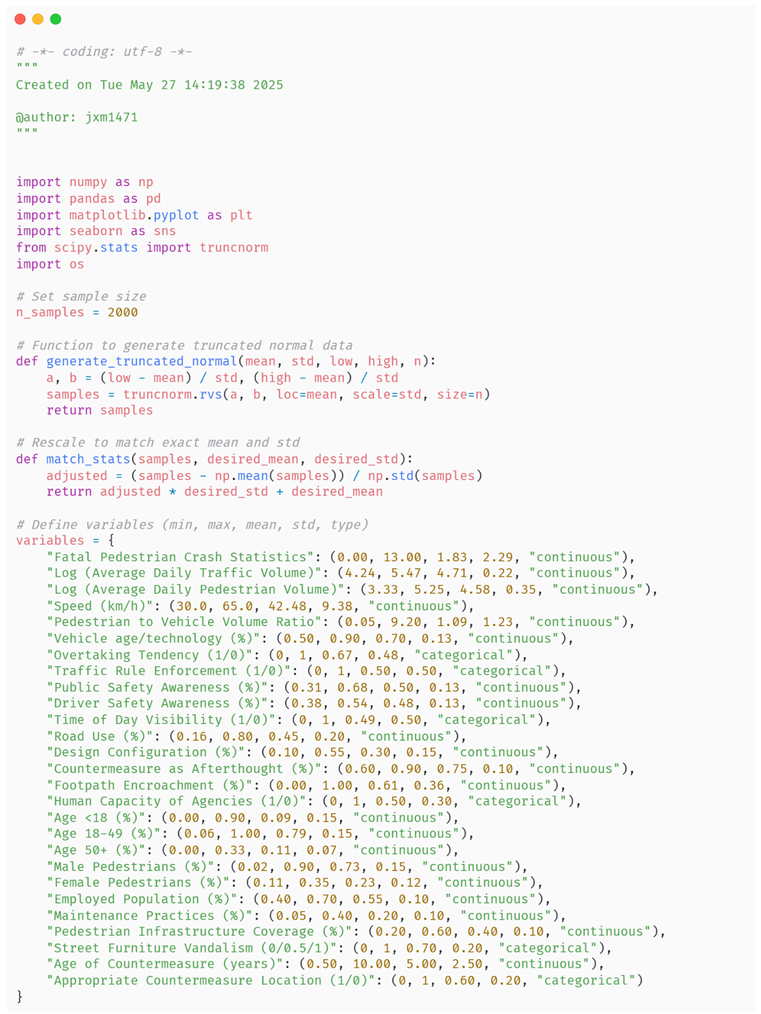
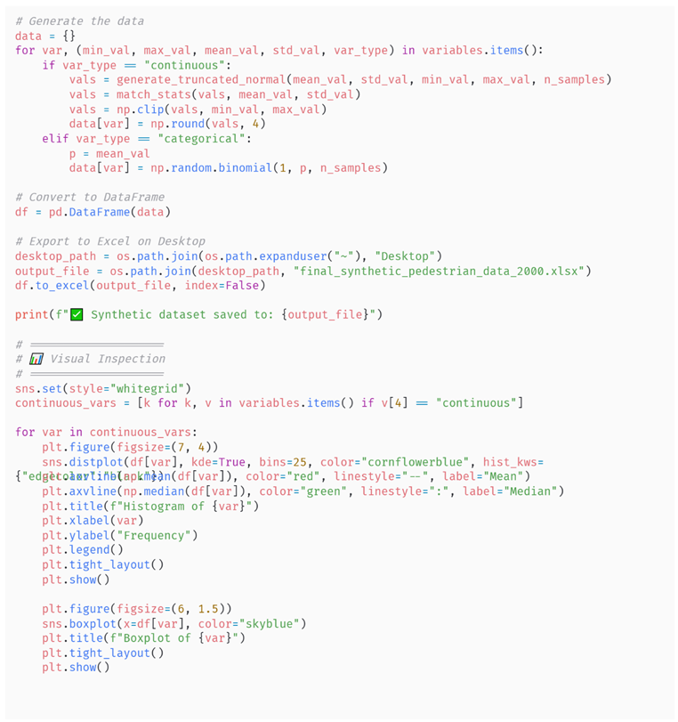
The generation process was implemented using Python (Spyder IDE) programming language with libraries including: NumPy for numerical random computation, SciPy for statistical distribution fitting, Pandas for dataset structuring, and Matplotlib for data visualisation [11].
The approach was designed to simulate realistic but artificial data distributions based on the following process:
- Used NumPy to generate 2000 random artificial data values for each variable. NumPy’s random number capabilities are widely used in scientific computing for simulation and statistical modelling tasks [12].
- To ensure statistical reliability, truncated normal distributions were applied on continuous variables to generate random numbers using SciPy’s truncnorm function [13]. This ensured that all values fall within the literature-derived minimum and maximum range while approximating the specified mean and standard deviation [14].
- Random binary distribution was used for Categorical/binary variables based on the reported mean values. This is equivalent to a Bernoulli random distribution [15].
- Normalised and rescaled the generated values to have nearly the same mean and standard deviation using Pandas [16].
- Generated histograms and boxplots using Matplotlib to visually verify variable distributions [17].
Outputs were cross-checked using Microsoft Excel for validation of randomisation patterns and value ranges.
The Python code used in generating the artificial data is indicated in Appendix A.
The summary of the generated artificial data distribution characteristics for each variable is presented in Table 2. The distribution checks inform of histograms and box plots for each factor are presented in Appendix B.
2.3. Estimating the Influence of Risk Factors on Pedestrian Crash Outcomes
Following the generation of the artificial data sets, this section focuses on applying correlation analysis and regression techniques to the artificial data to demonstrate how risk modelling could be operationalised.
2.3.1. Correlation Analyses
Spearman’s correlation was chosen because it evaluates the strength of monotonic relationships between variables based on ranked values [18]. It works well for mixed variable types because it’s non-parametric and only depends on ranks, not scale or distribution.
To calculate the correlation between each pair of variables, the following steps were followed:
- Ranked the values of the independent variable (X) across all the 2000 random observations. Replaced each row value for the variable with their corresponding ranks.
- Ranked the fatal pedestrian crash counts/ dependent variable (Y), across 2000 random observations.
- Calculated the Spearman’s correlation coefficient between the two ranked pairs of variables using the following correlation formula:
Where:
- ρ is the Spearman correlation coefficient,
- di is the difference in ranks between the two variables (e.g., di = rank(Xi) – rank(Yi))
- n is the number of observations (where n = 2000).
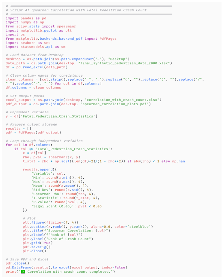
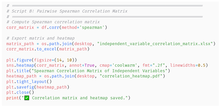
This technique was applied in two stages. First, Spearman’s rank correlation was used to evaluate the monotonic relationship between each independent variable and the dependent variable (fatal pedestrian crash count). The results of this analysis are presented in Table 3. Second, pairwise correlations were computed among each pair of variables to assess the presence of multicollinearity, with the results summarised in Table 4.
The Python scripts used to compute the Spearman correlation coefficients and generate the output tables for both steps are provided in Appendix C (1) and Appendix C(2), respectively.
These diagnostics were intentionally descriptive, not inferential, given the artificial nature of the data.
2.3.2. Stepwise Regression Modelling
Six Negative Binomial (NB) regression models were developed to predict fatal pedestrian crash frequencies. The NB model was chosen due to its ability to handle over-dispersed count data, where the variance exceeds the mean [19]. In this case, the variance (σ = 4.305) was greater than the mean (μ = 2.022).
According to Cameron and Trivedi [20], NB2 (quadratic variance) is the standard used in most crash-frequency modelling literature. It is also the default in Python’s statsmodels Generalised Linear Models (GLM) implementation, where variance increases quadratically with the mean. Therefore, under the NB2 parameterisation, the distribution of counts is defined as:
Where is the expected number of crashes at location I, and is the dispersion parameter.
The mean was linked to covariates through the canonical log link:
Where are predictor variables and are regression coefficients, estimated by maximum likelihood.
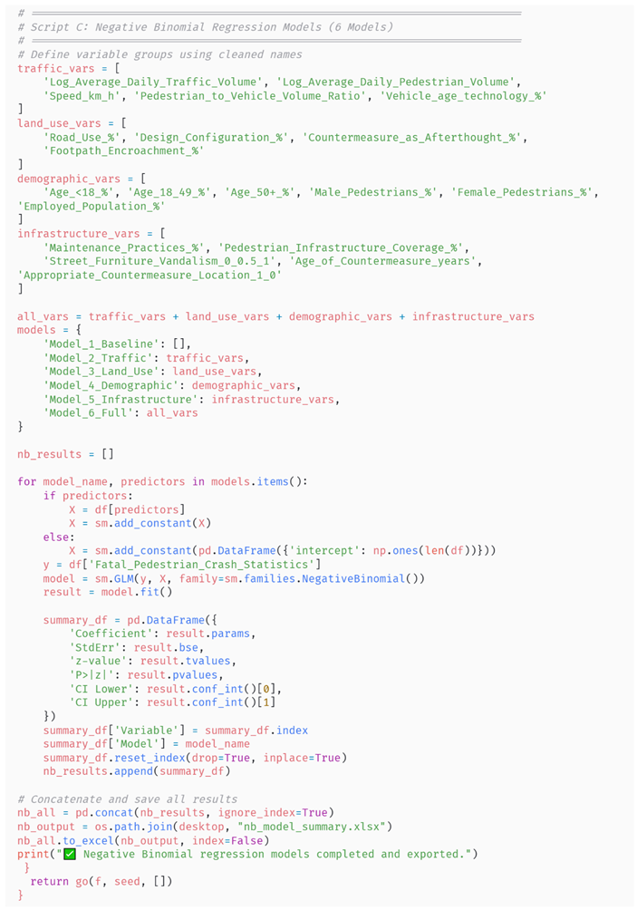
The 6 NB models were fitted according to the following predictor groups:
- Model 1: Constant only (baseline)
- Model 2: Traffic exposure and operational variables (e.g., Mixed traffic conditions)
- Model 3: Land use and planning variables (e.g., Road use)
- Model 4: Demographics (e.g., age group)
- Model 5: Infrastructure and roadway variables (e.g., coverage of pedestrian infrastructure)
- Model 6: Full model (combined all variables)
The general form for fitting the NB model on the artificial data was as follows:
Where:
- yi is the expected number of crashes/crash count at point i
- X1i, X2i, ….: independent/predictor variables.
- β0, β2, …: coefficients estimated by maximum likelihood.
Each coefficient βk corresponds to the log change in the expected crash count per one-unit increase in predictor Xk.
- Coefficients, Wald Statistics, and Significance Testing
Coefficients (βk)were estimated using Maximum Likelihood Estimation (MLE). They indicated the direction (+/-) and magnitude of association, which were interpreted using exponential transformation (exp βk), which gives the multiplicative effect on crash frequency. To assess significance / test whether a coefficient is significantly different from zero, Wald statistics were calculated as follows:
Where SE is the standard error of the coefficient.
A high absolute value (typically |z|> 1.96 at the 95% confidence level) indicates statistical significance.
- Dispersion Parameter (Alpha)
The Negative Binomial model introduces a dispersion parameter α to account for overdispersion as follows :
A non-zero α confirms overdispersion, and the NB is better than the Poisson
- Log-Likelihood Function and Goodness-of-Fit Metrics
The contribution of each observation to the NB log-likelihood, expressed using dispersion/shape , is:
Where LL is the log-likelihood function of convergence, and Γ is a gamma function.
The overall log-likelihood of the model (LLmodel) is the sum of the log-likelihoods of each site/observation (in this case, 2000 observations), given using the following formula:
Model adequacy was further evaluated using:
- Restricted Log-Likelihood () of the null (intercept-only) model
- McFadden’s Pseudo-R2 static / log-likelihood ratio index (ρ2) given by:
- Akaike Information Criterion (AIC), which is given as:
Equations 6,7,8,9 to 10 were formulated based on an adapted example of pedestrian risk modelling conducted in Kolkata, India, as presented by Mukherjee and Mitra [9]. Their work provided a practical foundation for structuring risk exposure and estimating the influence of contextual factors on crash frequency in data-challenged environments. This research builds upon and modifies that approach to reflect the operational realities of developing countries, thereby ensuring methodological relevance while leveraging an established framework.
It is important to note that each model was evaluated based on coefficient direction, relative magnitude, and thematic alignment, and not statistical significance.
- Implementation in Python
All models were fitted in Python using the statsmodels Generalised Linear Model (GLM) with a Negative Binomial family and log link. The Python code for fitting the 6 NB regression models and exporting model coefficients, standard error, p-values, and confidence intervals is detailed in Appendix D. The modelling outcomes are exhibited in Table 5.
2.3.3. Transforming NB Coefficients into Risk Factor Influence Values (Fi)
Exponential Transformation converted NB model coefficients into Factor Influence values (Fi) using the exponential function:
Where suggests increased risk, suggests a protective effect and suggests no effect.
These Fi values are equivalent to incident rate ratios (IRR). They indicate the multiplicative change in expected crash counts per one-unit increase in Xk. For this research, the Fi/IRR values were the point of interest and hence regarded as the risk factor values of interest. Risk factor values are presented as part of Table 6.
2.4. Comparative Analyses
A comparative analysis was conducted to assess which of the 33 variables identified in the unpublished systematic literature review (SLR) were represented in the negative binomial regression model and in the current iRAP pedestrian crash risk framework [21]. The objective was to pinpoint contextual factors found to be significant in the SLR but absent from both the NB model results and the existing iRAP framework. The comparison results are presented in Table 6.
3. Results
3.1. Distribution of Trend Data and Artificial Datasets for Each Factor
Table 1 presents the trend values (minimum, maximum, mean, standard deviation) for the variables as extracted from the literature, along with their sources. These values provided the statistical boundaries for generating artificial datasets.
Using distributions from Table 1 above, artificial datasets of 2,000 random samples per variable were generated in Python. The descriptive statistics of the generated datasets are summarised in Table 2, showing that the artificial data closely approximated the literature-derived boundaries while maintaining internal variability.
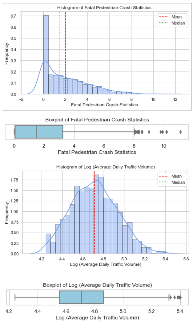
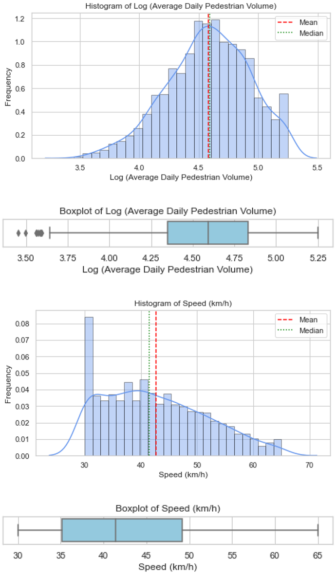
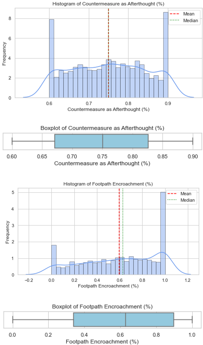
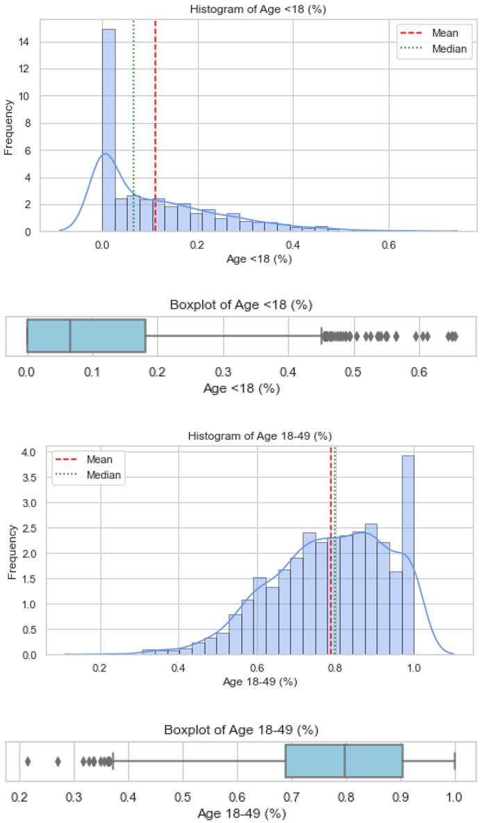
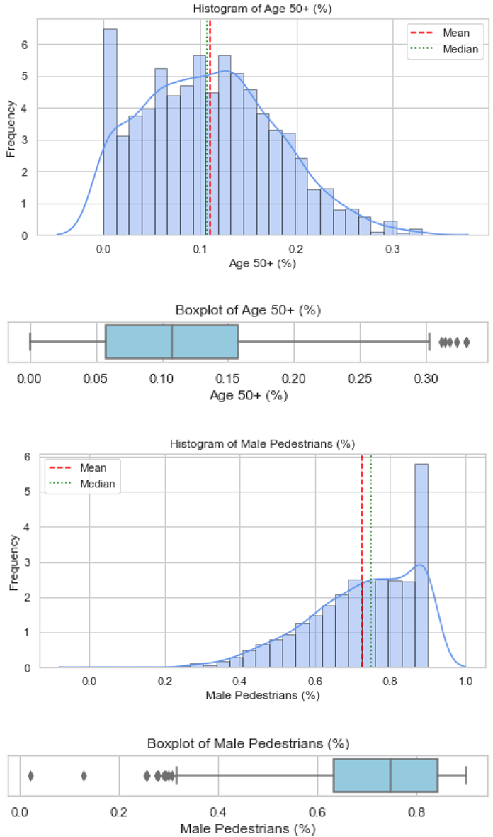
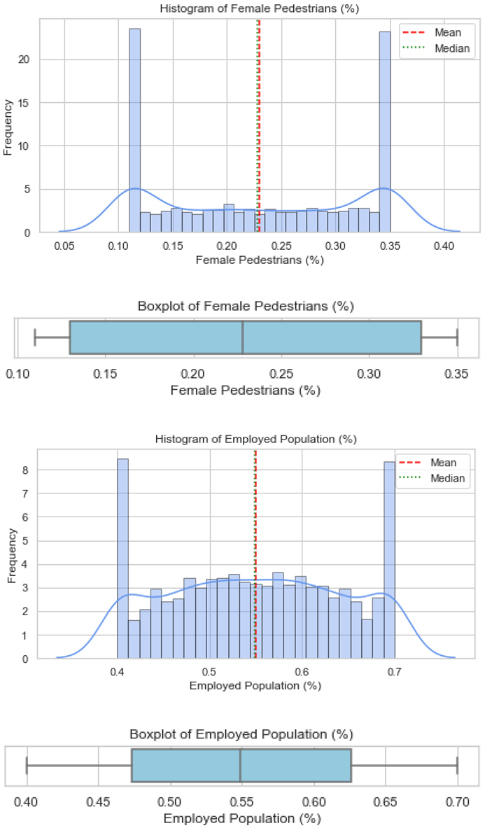
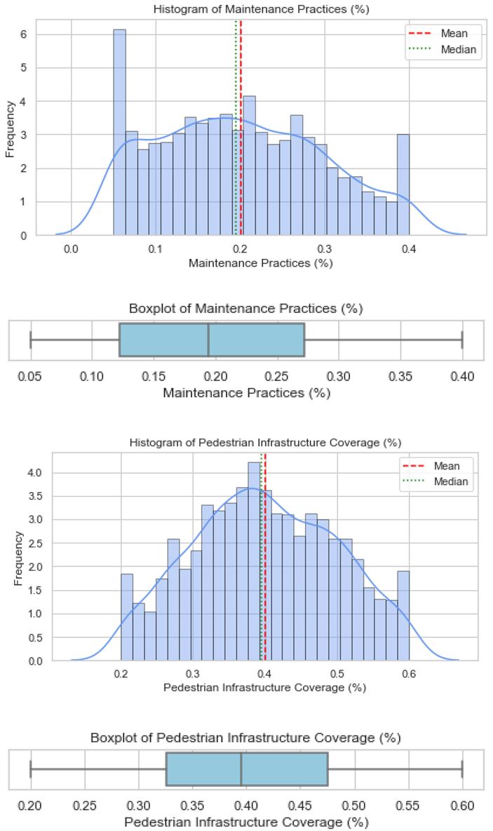
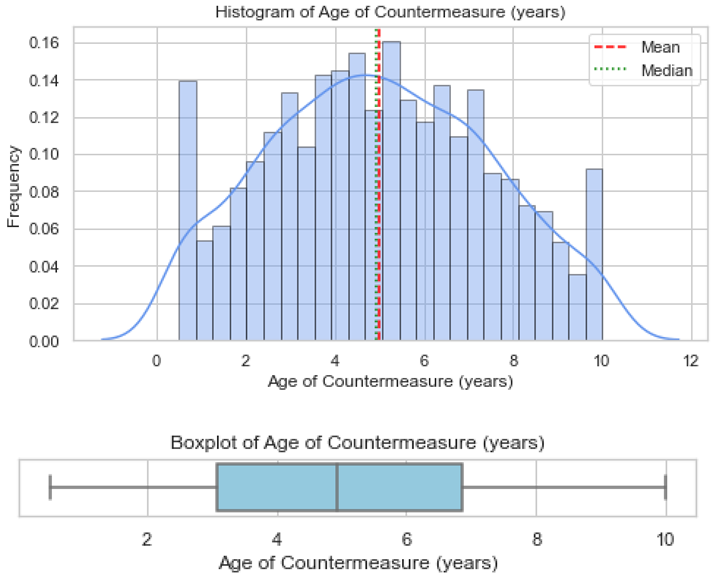
Validation of these datasets was undertaken using histograms and boxplots. For illustration, Figure 1 presents the distribution for Countermeasure as Afterthought, showing both the histogram and boxplot outputs, respectively. Similar plots were produced for all the factors and are provided in Appendix B. These visualisations confirm that the artificial datasets reflected realistic patterns and did not deviate from the empirical trends reported in the literature.
The histogram of the "Countermeasure as Afterthought (%)" variable shows a bimodal distribution, with peaks centred at approximately 0.6 and 0.9. This indicates that different areas take distinct approaches in implementing pedestrian safety countermeasures, with some relying heavily on retrospective measures, while others apply them only occasionally. Although the mean and median are both close to 0.75, this average may hide the two underlying patterns. To better visualise this, a Kernel Density Estimation (KDE) curve was used, which smooths the data and confirms the presence of two clear peaks. KDE is a non-parametric method used to estimate the probability density function of a continuous variable and is especially helpful for identifying multiple modes in a dataset without depending on histogram binning [40]. This pattern may reflect disparities in planning philosophies, with some jurisdictions prioritising pedestrian safety as a primary concern, while others address it only after an incident / as an afterthought. Such divergence may be rooted in differing regulatory environments, funding limitations, or urban planning priorities.
Overall, several variables (e.g., vehicle age, public safety awareness, female pedestrians, and employed population) exhibited bimodal or skewed distributions, reflecting heterogeneity in DC contexts, while others (e.g., pedestrian infrastructure coverage) showed near-normal patterns.
3.2. Correlation Analysis
Pairwise Spearman’s correlation results between each factor and pedestrian crash counts are presented in Table 3.
Although correlation magnitudes were generally weak (P > 0.005), directionally useful associations were evident. For example, traffic rule enforcement, driver safety awareness, and human capacity of agencies showed positive correlations with crash counts, while installing a countermeasure as an afterthought, overtaking tendency, and public safety awareness were negatively correlated.
Pairwise correlation among each pair of variables is reported in Table 4.
No strong correlations were observed between any two factors, indicating no evidence of multicollinearity among the independent variables
3.3. Regression Analysis (Negative Binomial Models)
Table 5 presents the outputs of the six Negative Binomial regression models fitted to the artificial datasets.
As expected, none of the modelled variables reached conventional statistical significance, reflecting the limitations of artificial datasets. Nonetheless, the NB coefficients provide useful inputs for transformation into risk factor influence values (Fi). Patterns in coefficient magnitudes suggested that demographic and institutional factors (e.g., employed population, human capacity of agencies) tended to exhibit higher potential influence compared with infrastructural factors, though this observation remains illustrative only.
3.4. Transforming NB Coefficients into Risk Factor Influence Values (Fi)
The six NB models produced varied β values, but none met the conventional threshold for statistical significance as mentioned earlier. Importantly, each model was evaluated based on coefficient direction, relative magnitude, and thematic alignment. The results, therefore, illustrate methodological feasibility rather than providing empirically validated estimates. The Fi values were calculated as the exponential transformation of NB coefficients (eβ), using equation 11.
Illustrative examples of Fi values included the following:
- Countermeasure as Afterthought had a risk factor value of 0.63, indicating a 37% reduction in expected safety benefits when countermeasures are implemented after an accident has happened rather than before.
- Female pedestrians had a risk factor value of 0.86, reinforcing gender-specific vulnerability that remains unaddressed in current global frameworks.
- Employed Population (1.22), and Age 18–49 (1.15) showed the highest positive risk values among demographic variables. These highlight that areas with a high concentration of working-age pedestrians face elevated pedestrian crash risks, even when standard countermeasures are applied.
- Vehicle Age/Technology (1.16) also exhibited an elevated risk value, pointing to the indirect effects of outdated or poorly maintained vehicle fleets, another non-iRAP parameter.
- Design Configuration (1.14) and Road Use (1.05), both geometric variables already covered in iRAP showed moderate risk increases. However, their explanatory power appeared weaker compared to social-behavioural and institutional variables.
More details can be found in Table 6, presented in the next section.

Table 6.
Comparison of SLR-identified variables, NB Inclusion, iRAP coverage, and Risk Factor Values (Fi).
Table 6.
Comparison of SLR-identified variables, NB Inclusion, iRAP coverage, and Risk Factor Values (Fi).
| Variable / factor | Coefficient (β) | P-value | Risk factor (Fi) = eβ | In NB Model | iRAP Covered | Practical Notes |
|---|---|---|---|---|---|---|
| Log (Avg Daily Traffic Volume) | -0.15 | 0.24 | 0.86 |  |
|
iRAP uses traffic flow |
| Log (Avg Daily Pedestrian Volume) | 0.10 | 0.19 | 1.11 | |
|
Pedestrian exposure proxy |
| Speed (km/h) | 0.00 | 0.42 | 1.00 | |
|
iRAP core attribute |
| Pedestrian/Vehicle Volume Ratio | 0.00 | 0.86 | 1.00 | |
 |
Not in iRAP |
| Vehicle Age / Technology (%) | 0.15 | 0.51 | 1.16 | |
|
Not in iRAP; age of fleet |
| Overtaking Tendency (1/0) | |
|
Critical in SLR only | |||
| Traffic Rule Enforcement (1/0) | |
|
Institutional variable | |||
| Public Safety Awareness (%) | |
|
Critical in SLR only | |||
| Driver Safety Awareness (%) | |
|
Critical in SLR only | |||
| Time of Day Visibility (1/0) | |
(Indirect) |
Lighting is a proxy | |||
| Road Use (%) | 0.05 | 0.73 | 1.05 | |
|
Functional classification included |
| Design Configuration (%) | 0.13 | 0.52 | 1.14 | |
|
Includes medians, crossings, etc. |
| Countermeasure as Afterthought (%) | -0.46 | 0.11 | 0.63 | |
|
Planning sequence not captured |
| Footpath Encroachment (%) | 0.00 | 0.99 | 1.00 | |
|
Informal sector factor |
| Human Capacity of Agencies (1/0) | |
|
Institutional capacity – not modeled | |||
| Age <18 (%) | 0.06 | 0.79 | 1.06 | |
|
covered under Star rating for schools |
| Age 18–49 (%) | 0.14 | 0.47 | 1.15 | |
|
High activity demographic |
| Age 50+ (%) | -0.08 | 0.83 | 0.92 | |
|
Vulnerable group not addressed |
| Male Pedestrians (%) | 0.11 | 0.57 | 1.12 | |
|
SLR demographic dimension |
| Female Pedestrians (%) | -0.15 | 0.61 | 0.86 | |
|
Gender exposure gap |
| Employed Population (%) | 0.20 | 0.49 | 1.22 | |
|
Mobility-related risk |
| Maintenance Practices (%) | -0.10 | 0.68 | 0.90 | |
(Indirect) |
Maintenance quality implied in iRAP |
| Pedestrian Infrastructure Coverage (%) | 0.07 | 0.84 | 1.07 | |
|
iRAP footpath attribute |
| Street Furniture Vandalism (0/0.5/1) | -0.03 | 0.65 | 0.97 | |
|
SLR-identified; social disorder indicator |
| Age of Countermeasure (years) | -0.01 | 0.36 | 0.99 | |
|
Asset age not considered in iRAP |
| Appropriate Countermeasure Location (1/0) | 0.04 | 0.41 | 1.04 | |
(Indirect) |
Part of iRAP’s star logic |
3.5. Comparative Analysis with iRAP Framework
The comparative analysis identified 16 contextual factors not currently included in iRAP’s pedestrian crash risk framework (Table 6).
Among these, five factors including overtaking tendency, traffic rule enforcement, public safety awareness, driver safety awareness, and human capacity of agencies, were neither captured in NB modelling outputs nor covered by iRAP. Their omission highlights potential blind spots in the current iRAP methodology, which may lead to overestimation of countermeasure performance in DC contexts.
4. Discussion
This paper demonstrated how literature trends and artificial data can be used to simulate modelling processes in data-constrained contexts. The results reflect a methodological process designed to assess risk relationships, not to infer statistical causality.
The methodological approach adopted offers a significant contribution to the study of pedestrian safety in data-scarce contexts by demonstrating how artificial datasets, informed by literature-derived parameters, can be used to model and analyse contextual risk factors. This is particularly relevant for developing countries (DCs), where empirical crash data is often unavailable, unreliable, or inconsistent across jurisdictions [7,41,42]. The use of structured simulations, grounded in peer-reviewed studies and grey literature, ensures that the synthetic data not only mirrors the statistical properties of real-world observations but also preserves contextual relevance [43].
The Spearman correlation analysis and subsequent Negative Binomial (NB) regression modelling revealed several noteworthy patterns. While statistical significance could not be meaningfully assessed, owing to the absence of real-world inter-variable dependencies, the practical implications of the derived risk values (Fi) were evident. Notably, behavioural and institutional variables such as Countermeasure as an Afterthought[8], Female Pedestrian Proportion [44], and Vehicle Age/Technology[45] displayed stronger risk factors than several geometric variables already embedded within the iRAP framework. This highlights the systemic oversight of socio-behavioural determinants in mainstream road safety assessment tools and supports previous critiques that global frameworks often inadequately represent the urban complexities of low- and middle-income countries [21,46–48].
Moreover, the comparative analysis between the NB included variables, iRAP attributes, and the 33 systematic literature review (SLR) findings reveals important thematic misalignments. While iRAP effectively captures geometric design and speed parameters, it largely omits contextual and behavioural dimensions such as Traffic Rule Enforcement, Public Safety Awareness, and Institutional Capacity [48,49]. These omissions likely contribute to the persistent "effectiveness gap" observed in the implementation of safety countermeasures in DCs. This aligns with David Freeman [41] and Washington, Karlaftis [50], who argue that globalised safety models often fail to account for the diverse urban realities of DC contexts.
The creation of multiple NB models grouped by variable typology (exposure, land use, demographics, and infrastructure) also provided insight into domain-specific influences on crash frequency. Although infrastructure variables demonstrated a logical alignment with iRAP, their risk values were generally lower compared to demographic and institutional variables, suggesting that the highest safety returns may come from broader governance and behavioural reforms rather than physical redesign alone [8,48]. This reflects a shift in thinking within the urban transport safety community, where "soft" interventions like awareness, compliance, and institutional reforms are increasingly acknowledged as vital complements to traditional engineering solutions [7,44].
Furthermore, the artificial dataset served not only as a methodological bridge but also as a platform to test the viability of incorporating underrepresented variables into predictive modelling frameworks. Despite inherent limitations such as a lack of empirical validation and potential overfitting, the study successfully demonstrated that credible and reproducible risk models can be developed using literature-informed simulation [8,43]. The structured generation process, using Python-based statistical libraries like NumPy and SciPy, ensured adherence to statistical principles while enabling traceability, a critical component in transparent data analysis practice.
Notably, this study not only provides a foundational proof-of-concept for contextualised risk modelling in the absence of empirical data but also surfaces important systemic gaps in current global road safety evaluation tools. These insights can be directly operationalised in future, where a new context-adjusted iRAP effectiveness variant model is proposed. This model integrates both the empirical weightings derived from NB regression and literature-based weights for variables excluded from the regression but deemed important in the SLR. This integrative approach aims to enhance the sensitivity and relevance of pedestrian safety assessments in developing countries [42,48].
While the current iRAP model addresses the statistical modelling of crash outcomes and injury severities, the methodological innovation suggested in future should take a different but complementary direction. It should address the predictive limitations of generic effectiveness models and demonstrate the value of localised parameterisation [49,51].
5. Conclusions and Recommendations
This study demonstrates that artificially generated datasets, informed by literature-derived distributions, can effectively identify and rank contextual risk factors influencing pedestrian crash risk in DCs. The resulting Fi values highlight critical gaps in existing global models, including the omission of socio-spatial and behavioural factors that significantly shape safety outcomes in low-resource environments.
This methodological demonstration shows how artificial datasets, when carefully constructed, can support the preliminary assessment of contextual factors influencing pedestrian crash risk in data-scarce settings like in DCs. Key findings include:
- Confirmation that several high-impact factors are not represented in iRAP’s pedestrian crash risk model.
- Identification of both modelled and unmodelled variables absent from iRAP that merit further empirical investigation.
However, as the current outputs are based on simulated data, empirical calibration is essential before operational use in policy or infrastructure prioritisation.
- Future work should:
- Apply the framework to real-world DC crash datasets for calibration.
- Incorporate missing high-impact variables into iRAP’s model.
- Develop regionally adaptive countermeasure prioritisation tools for use in national safety plans.
Author Contributions
Conceptualization, J.M. and H.E.; methodology, analysis, and writing, J.M.; supervision, H.E. All authors have read and agreed to the published version of the manuscript.
Funding
This research received no external funding.
Institutional Review Board Statement
Not applicable
Informed Consent Statement
Any Not applicable
Data Availability Statement
The data supporting the reported results can be obtained from the corresponding author upon reasonable request.
Acknowledgments
The authors would like to acknowledge the support of the Commonwealth Scholarship Commission, and the University of Birmingham for providing the necessary resources.
Conflicts of Interest
The authors declare no conflict of interest.
Abbreviations
The following abbreviations are used in this manuscript:
| DC | Developing Country |
| GLM | Generalised Linear Model |
| HIC | High-Income Country |
| IDE | Integrated Development Environment |
| iRAP | International Road Assessment Programme |
| KDE | Kernel Density Estimation |
| NB | Negative Binomial |
| SLR | Systematic Literature Review |
| WHO | World Health Organisation |
Appendix A
Appendix A: Python Code for Generating Artificial Data for all the Variables
Appendix B
Appendix B: Histograms and Boxplots Showing Distribution for Various Variables
Appendix C
Appendix C(1): Python Code That Generated Spearman’s Correlation of the Independent Variables with Pedestrian Crash Counts
Appendix C(2): Python Code Used to Generate the Pairwise Spearman’s Correlation Between Independent Variables
Appendix D
Appendix D: Python Code for Developing Negative Binomial Regression Models
References
- WHO, Pedestrian safety: a road safety manual for decision-makers and practitioners. 2023: World Health Organisation.
- Karathodorou, N. Development of a crash modification factors model in Europe. in 17th International Conference Road Safety On Five Continents (RS5C 2016), Rio de Janeiro, Brazil, 17-19 May 2016. 2016. Statens väg-och transportforskningsinstitut.
- National Academies of Sciences, E. , and Medicine,, Pedestrian Safety Prediction Methodology. 2008, Washington, DC: The National Academies Press. 0.
- Kraidi, R. and H. Evdorides, Pedestrian safety models for urban environments with high roadside activities. Safety Science, 2020. 130: p. 104847. [CrossRef]
- Job, R.S. and W.M. Wambulwa, Features of low-income and middle-income countries making road safety more challenging. Journal of road safety, 2020. 31(3): p. 79-84.
- Thierry, M. , et al., A New Methodology for Road Crash Data Collection in Bangladesh Using Local Record Keepers. Journal of Road Safety, 2023. 34: p. 1-11. [CrossRef]
- Lin, P.-S. , et al., Development of countermeasures to effectively improve pedestrian safety in low-income areas. Journal of Traffic and Transportation Engineering (English Edition), 2019. 6(2): p. 162-174. [CrossRef]
- Mukherjee, D. and S. Mitra, Identification of Pedestrian Risk Factors Using Negative Binomial Model. Transportation in Developing Economies, 2020. 6(1): p. 4. [CrossRef]
- Mukherjee, D. and S. Mitra, Modelling risk factors for fatal pedestrian crashes in Kolkata, India. Int J Inj Contr Saf Promot, 2020. 27(2): p. 197-214. [CrossRef]
- Parker, C. Scott, and A. Geddes, Snowball sampling. SAGE research methods foundations, 2019.
- Sundaram, J. , et al., An Exploration of Python Libraries in Machine Learning Models for Data Science, in Advanced Interdisciplinary Applications of Machine Learning Python Libraries for Data Science, S.M. Biju, A. Mishra, and M. Kumar, Editors. 2023, IGI Global Scientific Publishing: Hershey, PA, USA. p. 1-31.
- Harris, C.R. , et al., Array programming with NumPy. Nature, 2020. 585(7825): p. 357-362. [CrossRef]
- Virtanen, P. , et al., SciPy 1.0: fundamental algorithms for scientific computing in Python. Nature Methods, 2020. 17(3): p. 261-272.
- Freedman, D.A. , Statistical models: theory and practice. 2009: cambridge university press.
- Lee, A. , Generating random binary deviates having fixed marginal distributions and specified degrees of association. The American Statistician, 1993. 47(3): p. 209-215.
- McKinney, W. , Python for data analysis: Data wrangling with Pandas, NumPy, and IPython. 2012: " O'Reilly Media, Inc.".
- Yim, A. Chung, and A. Yu, Matplotlib for Python Developers: Effective techniques for data visualization with Python. 2018: Packt Publishing Ltd.
- Hauke, J. and T. Kossowski, Comparison of values of Pearson's and Spearman's correlation coefficients on the same sets of data. Quaestiones geographicae, 2011. 30(2): p. 87-93.
- Mukherjee, D. and S. and Mitra, Pedestrian safety analysis of urban intersections in Kolkata, India using a combined proactive and reactive approach. Journal of Transportation Safety & Security, 2022. 14(5): p. 754-795. [CrossRef]
- Cameron, A.C. and P.K. Trivedi, Regression analysis of count data. 2013: Cambridge university press.
- iRAP. iRAP Specification, Manuals and Guides. 2021 31/07/2025]; Available from: https://irap.org/specifications/.
- Earth.Org. Millions of Highly-Polluting Used Cars “Dumped” on Developing Countries- UN. 2020 [cited 2025 15/08/2025]; Available from: https://earth.org/cars-developing-countries/.
- Heydari, S. , et al., Road safety in low-income countries: state of knowledge and future directions. Sustainability, 2019. 11(22): p. 6249. [CrossRef]
- Chowdhury, T. M. Rifaat, and R. Tay, Characteristics of Pedestrians in Bangladesh Who Did Not Receive Public Education on Road Safety. Sustainability, 2022. 14(16): p. 9909. [CrossRef]
- Shaaban, K. , Impact of experience and training on traffic knowledge of young drivers. The Open Transportation Journal, 2021. 15(1). [CrossRef]
- Mukherjee, D. and S. Mitra, Comprehensive Study of Risk Factors for Fatal Pedestrian Crashes in Urban Setup in a Developing Country. Transportation Research Record, 2020. 2674(8): p. 100-118. [CrossRef]
- Victoria Transport Policy Institute. Developing Country Developing Country Transport Demand Management: Transportation Demand Management in Lower-Income Regions. 2019 [cited 2025 15/08/2025]; Available from: https://www.vtpi.org/tdm/tdm75.htmDemand Management: Transportation Demand Management in Lower-Income Regions.
- Frimpong, L.K. Enhancing Pedestrian Safety in African Cities. 2022 15/08/2025]; Available from: https://www.researchgate.net/publication/363415723_Enhancing_Pedestrian_Safety_in_African_Cities#fullTextFileContent.
- Jia, W. B. Tesfaye, and Y.M. Alcala. How can we make cities safer for pedestrians? Some insights from Ethiopia. 2022 [cited 2025 15/08/2025]; Available from: https://blogs.worldbank.org/en/transport/how-can-we-make-cities-safer-pedestrians-some-insights-ethiopia.
- Walelign Bishaw, T. Nurye Dolebo, and R.B. Singh, Evaluating pedestrian facilities for enhancing pedestrian safety in Addis Ababa city. Frontiers in Sustainable Cities, 2024. Volume 6 - 2024. [CrossRef]
- Damsere-Derry, J. , et al., Evaluation of the effectiveness of traffic calming measures on vehicle speeds and pedestrian injury severity in Ghana. Traffic Injury Prevention, 2019. 20(3): p. 336-342. [CrossRef]
- Osuret, J. , et al., State of pedestrian road safety in Uganda: a qualitative study of existing interventions. Afr Health Sci, 2021. 21(3): p. 1498-1506. [CrossRef]
- Sabi Boun, S. , et al., Environmental measures to improve pedestrian safety in low- and middle-income countries: a scoping review. Glob Health Promot, 2024: p. 17579759241241513. [CrossRef]
- Times News Network. Pedestrian life a no-go in Bhopal as BMC sidesteps duties & fails to walk the talk. 2025 [cited 2025 15/08/2025]; Available from: https://timesofindia.indiatimes.com/city/bhopal/pedestrian-life-a-no-go-in-bhopal-as-bmc-sidesteps-duties-fails-to-walk-the-talk/articleshow/121241233.cms.
- Bliss, T. and J.M. Breen, Road Safety Management Capacity Reviews and Safe System Projects Guidelines (Updated Edition). 2013: Washington, DC.
- Zhu, M. , et al., Why more male pedestrians die in vehicle-pedestrian collisions than female pedestrians: a decompositional analysis. Inj Prev, 2013. 19(4): p. 227-31. [CrossRef]
- International Labour Organization. Labor force participation rate, total (% of total population ages 15+) (modeled ILO estimate). 2025 [cited 2025 15/08/2025]; Available from: https://data.worldbank.org/indicator/SL.TLF.CACT.ZS.
- Arisoy, N. , Measuring students’ preferences for urban furniture vandalism in Selçuk University Campus in Turkey: A case study. Archives of Agriculture and Environmental Science, 2020. 5(3): p. 426-430. [CrossRef]
- Transportation Research Board, E. National Academies of Sciences, and Medicine, Development of Crash Modification Factors for Uncontrolled Pedestrian Crossing Treatments, ed. C. Zegeer, et al. 2017, Washington, DC: The National Academies Press. 162.
- Silverman, B.W. , Density estimation for statistics and data analysis. 1986: Routledge. [CrossRef]
- David Freeman, R.P. , and Roger Purves, Statistics Fourth Edition. 2007: W.W. Norton & Company.
- Zafri, N.M. and A. Khan, A spatial regression modeling framework for examining relationships between the built environment and pedestrian crash occurrences at macroscopic level: A study in a developing country context. Geography and Sustainability, 2022. 3(4): p. 312-324. [CrossRef]
- Huang, H. and M. Abdel-Aty, Multilevel data and Bayesian analysis in traffic safety. Accident Analysis & Prevention, 2010. 42(6): p. 1556-1565. [CrossRef]
- Yang, J. , et al., Examining the Factors Influencing Pedestrian Behaviour and Safety: A Review with a Focus on Culturally and Linguistically Diverse Communities. Sustainability, 2025. 17(13): p. 6007. [CrossRef]
- Ghasedi, M. Sarfjoo, and I. Bargegol, Prediction and Analysis of the Severity and Number of Suburban Accidents Using Logit Model, Factor Analysis and Machine Learning: A case study in a developing country. SN Applied Sciences, 2021. 3(1): p. 13. [CrossRef]
- Mukherjee, D. and S. Mitra, A comprehensive study on factors influencing pedestrian signal violation behaviour: Experience from Kolkata City, India. Safety Science, 2020. 124. [CrossRef]
- Tiwari, G. , Progress in pedestrian safety research. International Journal of Injury Control and Safety Promotion, 2020. 27(1): p. 35-43. [CrossRef]
- Hossain, S. Maggi, and A. Vezzulli, Factors influencing the road accidents in low and middle-income countries: a systematic literature review. International journal of injury control and safety promotion, 2024. 31(2): p. 294-322. [CrossRef]
- Mukherjee, D. , Analyzing key determinants of pedestrian risky behaviors at urban signalized intersections: insights from Kolkata City, India. International Journal of Injury Control and Safety Promotion, 2025. 32(2): p. 201-229. [CrossRef]
- Washington, S. , et al., Statistical and econometric methods for transportation data analysis. 2020: Chapman and Hall/CRC.
- Anis, M. R. Geedipally, and D. Lord, Pedestrian crash causation analysis near bus stops: Insights from random parameters NB-Lindley models. 2024; arXiv:2410.22253. [Google Scholar]
Disclaimer/Publisher’s Note: The statements, opinions and data contained in all publications are solely those of the individual author(s) and not of MDPI and/or the editor(s). MDPI and/or the editor(s) disclaim responsibility for any injury to people or property resulting from any ideas, methods, instructions or products referred to in the content. |
Figure 1.
(a) Histogram showing the distribution of countermeasure as an afterthought. (b): Boxplot showing the distribution of countermeasure as an afterthought.
Figure 1.
(a) Histogram showing the distribution of countermeasure as an afterthought. (b): Boxplot showing the distribution of countermeasure as an afterthought.
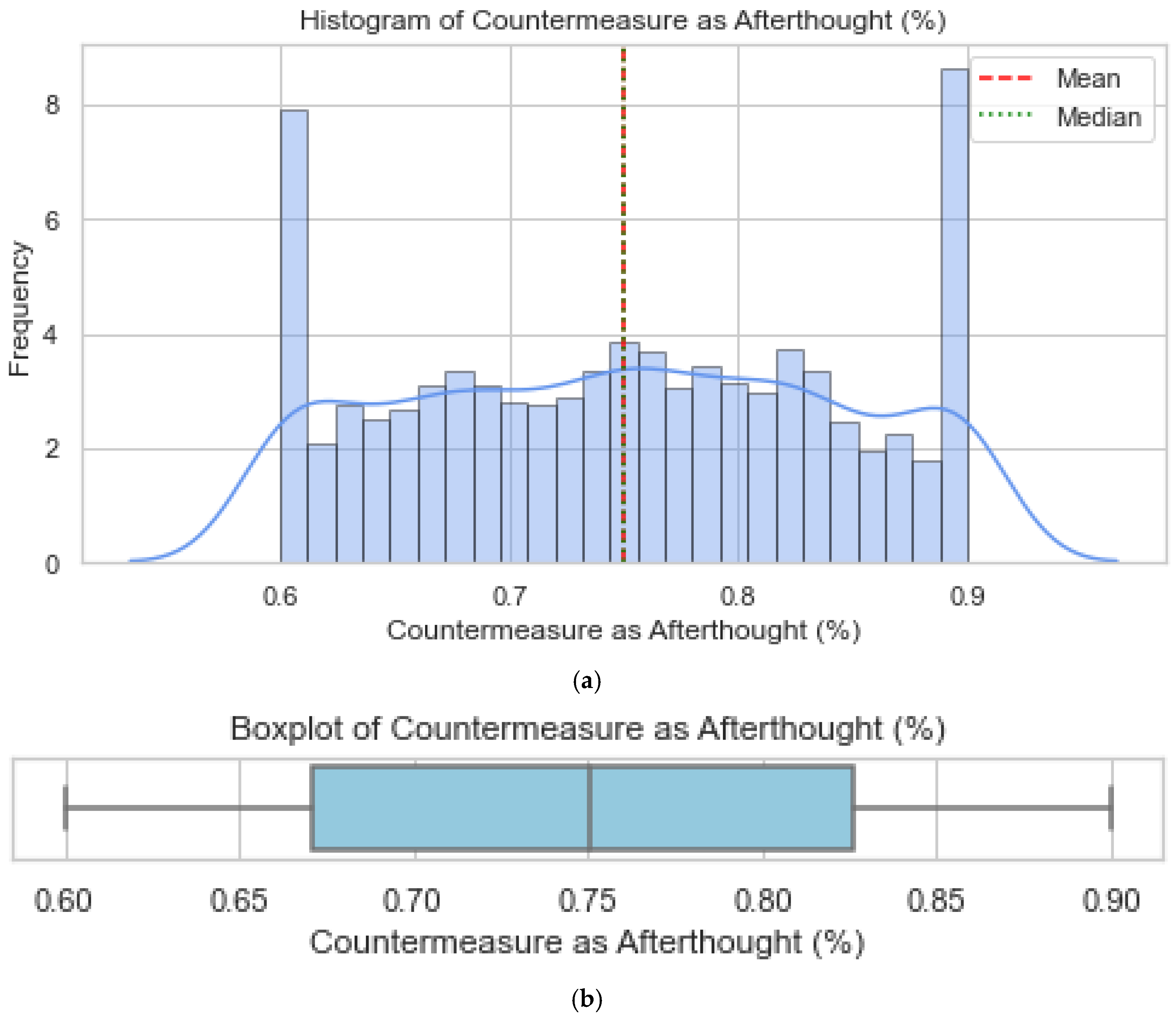
Table 1.
Literature-based frequency data characteristics for the different variables.
| Characteristics | Variables | Variable type | Minimum | Maximum | Mean (μ) | Standard Deviation (δ) | Reference | Country |
|---|---|---|---|---|---|---|---|---|
| Safety Performance | Fatal Pedestrian Crash Statistics | Continous | 0.00 | 13.00 | 1.83 | 2.29 | [9] | India |
| Traffic Exposures and Operational Characteristics | Log (Average Daily Traffic Volume) | Continous | 4.24 | 5.47 | 4.71 | 0.22 | [9] | India |
| Log (Average Daily Pedestrian Volume) | Continous | 3.33 | 5.25 | 4.58 | 0.35 | [9] | India | |
| Speed (km/h) | Continous | 30.00 | 65.00 | 42.48 | 9.38 | [9] | India | |
| Pedestrian to Vehicle Volume Ratio / Mixed Traffic Conditions | Continous | 0.05 | 9.20 | 1.09 | 1.23 | [9] | India | |
| Vehicle age/technology (%) | Continous | 0.50 | 0.90 | 0.70 | 0.13 | [22] | Nigeria, Ghana, Ethiopia, Kenya | |
| Compliance/ Presence of Overtaking Tendency of Vehicle (1/0) | Categorical | 0.00 | 1.00 | 0.67 | 0.48 | [9] | India | |
| Enforcement of Traffic rules (Yes = 1; No = 0) | Categorical | 0.00 | 1.00 | 0.50 | 0.50 | [9,23] | India | |
| Public safety awareness level (%) | Continous | 0.31 | 0.68 | 0.50 | 0.13 | [24] | Bangladesh | |
| Driver safety awareness level (%) | Continous | 0.38 | 0.54 | 0.48 | 0.13 | [25] | Quatar | |
| Time of the Day (visibility) (1/0) | Categorical | 0.00 | 1.00 | 0.49 | 0.50 | [26] | India | |
| Land use and Planning | Hierarchical Road Classification/Road Use (%) | Continous | 0.16 | 0.80 | 0.45 | 0.20 | [27] | Brazil, Columbia, Tanzania |
| Design Configuration (%) | Continous | 0.10 | 0.55 | 0.30 | 0.15 | [28–30] | Ethiopia, India | |
| Countermeasure as an afterthought (%) | Continous | 0.60 | 0.90 | 0.75 | 0.10 | [31–34] | Uganda, India, Ghana | |
| Encroachment of Footpath by Street vendors (%) | Continous | 0.00 | 1.00 | 0.61 | 0.36 | [9] | India | |
| Human Capacity of responsible agencies (Adequate = 1, Poor = 0) | Categorical | 0.00 | 1.00 | 0.50 | 0.30 | [35] | World Bank | |
| Demographics | Age group (%) | Below 18 years (%) | 0.00 | 0.90 | 0.09 | 0.15 | [26] | India |
| 18 - 49 years (in %) | 0.06 | 1.00 | 0.79 | 0.15 | [26] | India | ||
| 50+ years (%) | 0.00 | 0.33 | 0.11 | 0.07 | [26] | India | ||
| Gender (%) | Male pedestrians (%) | 0.02 | 0.90 | 0.73 | 0.15 | [26] | India | |
| Female (%) | 0.11 | 0.35 | 0.23 | 0.12 | [36] | USA | ||
| Employed population (%) | Continous | 0.40 | 0.70 | 0.55 | 0.10 | [37] | World Bank | |
| Infrastructure and Roadway Factors | Maintenance Practices/level (%) | Continous | 0.05 | 0.40 | 0.20 | 0.10 | [28,29] | Ghana & Ethiopia |
| Coverage of pedestrian infrastructure (%) | Continous | 0.20 | 0.60 | 0.40 | 0.10 | [34] | India | |
| Vandalism of Street Furniture (Never = 1; Sometimes = 0.5; Always = 0) | Categorical | 0.00 | 1.00 | 0.70 | 0.20 | [38] | Turkey | |
| Age of the countermeasure (years) | Continous | 0.50 | 10.00 | 5.00 | 2.50 | [39] | USA | |
| Appropriate location of countermeasure (1/0) | Categorical | 0.00 | 1.00 | 0.60 | 0.20 | [30] | Ethiopia |
Table 2.
Summary of generated artificial data characteristics for each variable.
| Characteristics | Variables | Variable type | Minimum | Maximum | Mean (μ) | Median | Standard Deviation (δ) |
|---|---|---|---|---|---|---|---|
| Safety Performance | Fatal Pedestrian Crash Statistics | Continous | 0.00 | 10.67 | 2.03 | 1.50 | 2.06 |
| Traffic Exposures and Operational Characteristics | Log (Average Daily Traffic Volume) | Continous | 4.24 | 5.47 | 4.71 | 4.71 | 0.22 |
| Log (Average Daily Pedestrian Volume) | Continous | 3.37 | 5.25 | 4.58 | 4.59 | 0.35 | |
| Speed (km/h) | Continous | 30.00 | 65.00 | 42.67 | 42.00 | 9.06 | |
| Pedestrian to Vehicle Volume Ratio / Mixed Traffic Conditions | Continous | 0.05 | 6.07 | 1.19 | 0.95 | 1.11 | |
| Vehicle age/technology (%) | Continous | 0.50 | 0.90 | 0.70 | 0.70 | 0.12 | |
| Compliance/ Presence of Overtaking Tendency of Vehicle (1/0) | Categorical | 0.00 | 1.00 | 0.66 | 1.00 | 0.48 | |
| Enforcement of Traffic rules (Yes = 1; No = 0) | Categorical | 0.00 | 1.00 | 0.51 | 1.00 | 0.50 | |
| Public safety awareness level (%) | Continous | 0.31 | 0.68 | 0.50 | 0.50 | 0.12 | |
| Driver safety awareness level (%) | Continous | 0.38 | 0.54 | 0.47 | 0.49 | 0.07 | |
| Time of the Day (visibility) (1/0) | Categorical | 0.00 | 1.00 | 0.48 | 0.00 | 0.50 | |
| Land use and Planning | Hierarchical Road Classification/Road Use (%) | Continous | 0.16 | 0.80 | 0.45 | 0.44 | 0.19 |
| Design Configuration (%) | Continous | 0.10 | 0.55 | 0.30 | 0.29 | 0.14 | |
| Countermeasure as an afterthought (%) | Continous | 0.60 | 0.90 | 0.75 | 0.75 | 0.09 | |
| Encroachment of Footpath by Street vendors (%) | Continous | 0.00 | 1.00 | 0.60 | 0.64 | 0.32 | |
| Human Capacity of responsible agencies (Adequate = 1, Poor = 0) | Categorical | 0.00 | 1.00 | 0.50 | 0.00 | 0.50 | |
| Demographics | Age group (%) | Below 18 years (%) | 0.00 | 0.69 | 0.11 | 0.07 | 0.13 |
| 18 - 49 years (in %) | 0.21 | 1.00 | 0.79 | 0.80 | 0.15 | ||
| 50+ years (%) | 0.00 | 0.33 | 0.11 | 0.10 | 0.07 | ||
| Gender (%) | Male pedestrians (%) | 0.13 | 0.90 | 0.72 | 0.74 | 0.14 | |
| Female (%) | 0.11 | 0.35 | 0.23 | 0.23 | 0.09 | ||
| Employed population (%) | Continous | 0.40 | 0.70 | 0.55 | 0.55 | 0.09 | |
| Infrastructure and Roadway Factors | Maintenance Practices/level (%) | Continous | 0.05 | 0.40 | 0.20 | 0.20 | 0.10 |
| Coverage of pedestrian infrastructure (%) | Continous | 0.20 | 0.60 | 0.40 | 0.40 | 0.10 | |
| Vandalism of Street Furniture (Never = 1; Sometimes = 0.5; Always = 0) | Categorical | 0.00 | 1.00 | 0.70 | 1.00 | 0.46 | |
| Age of the countermeasure (years) | Continous | 0.50 | 10.00 | 5.01 | 5.04 | 2.47 | |
| Appropriate location of countermeasure (1/0) | Categorical | 0.00 | 1.00 | 0.61 | 1.00 | 0.49 |
Table 3.
Spearman Correlation Between Independent Variables and Pedestrian Crash Count.
| Variable | Min | Max | Mean | Std Dev | Spearman Rho | T-Statistic | P-Value |
|---|---|---|---|---|---|---|---|
| Log Average Daily Traffic Volume | 4.240 | 5.470 | 4.710 | 0.220 | -0.029 | -1.285 | 0.199 |
| Log Average Daily Pedestrian Volume | 3.364 | 5.250 | 4.580 | 0.349 | 0.030 | 1.336 | 0.182 |
| Speed (km/h) | 30.000 | 65.000 | 42.697 | 8.988 | 0.029 | 1.282 | 0.200 |
| Pedestrian to Vehicle Volume Ratio | 0.050 | 6.087 | 1.179 | 1.128 | 0.000 | 0.010 | 0.992 |
| Vehicle age technology (%) | 0.500 | 0.900 | 0.700 | 0.122 | 0.003 | 0.124 | 0.901 |
| Overtaking Tendency (1/0) | 0.000 | 1.000 | 0.668 | 0.471 | -0.037 | -1.662 | 0.097 |
| Traffic Rule Enforcement (1/0) | 0.000 | 1.000 | 0.517 | 0.500 | 0.009 | 0.387 | 0.699 |
| Public Safety Awareness (%) | 0.310 | 0.680 | 0.499 | 0.119 | -0.026 | -1.161 | 0.246 |
| Driver Safety Awareness (%) | 0.380 | 0.540 | 0.468 | 0.069 | 0.017 | 0.755 | 0.450 |
| Time of Day Visibility (1/0) | 0.000 | 1.000 | 0.491 | 0.500 | 0.011 | 0.490 | 0.624 |
| Road Use (%) | 0.160 | 0.800 | 0.452 | 0.191 | 0.001 | 0.039 | 0.969 |
| Design Configuration (%) | 0.100 | 0.550 | 0.302 | 0.139 | 0.018 | 0.791 | 0.429 |
| Countermeasure as Afterthought (%) | 0.600 | 0.900 | 0.751 | 0.094 | -0.032 | -1.407 | 0.160 |
| Footpath Encroachment (%) | 0.000 | 1.000 | 0.596 | 0.326 | 0.008 | 0.342 | 0.733 |
| Human Capacity of Agencies (1/0) | 0.000 | 1.000 | 0.498 | 0.500 | 0.013 | 0.581 | 0.562 |
| Age <18 (%) | 0.000 | 0.685 | 0.111 | 0.128 | -0.021 | -0.926 | 0.355 |
| Age 18 - 49 (%) | 0.181 | 1.000 | 0.788 | 0.147 | 0.031 | 1.373 | 0.170 |
| Age 50+ (%) | 0.000 | 0.330 | 0.111 | 0.069 | -0.011 | -0.487 | 0.627 |
| Male Pedestrians (%) | 0.158 | 0.900 | 0.725 | 0.143 | 0.036 | 1.616 | 0.106 |
| Female Pedestrians (%) | 0.110 | 0.350 | 0.230 | 0.092 | -0.023 | -1.016 | 0.310 |
| Employed Population (%) | 0.400 | 0.700 | 0.550 | 0.094 | 0.021 | 0.947 | 0.344 |
| Maintenance Practices (%) | 0.050 | 0.400 | 0.201 | 0.097 | -0.006 | -0.251 | 0.802 |
| Pedestrian Infrastructure Coverage (%) | 0.200 | 0.600 | 0.400 | 0.099 | 0.008 | 0.374 | 0.709 |
| Street Furniture Vandalism (0/0.5/1) | 0.000 | 1.000 | 0.680 | 0.467 | -0.024 | -1.074 | 0.283 |
| Age of Countermeasure years | 0.500 | 10.000 | 5.006 | 2.466 | -0.022 | -0.968 | 0.333 |
| Appropriate Countermeasure Location (1/0) | 0.000 | 1.000 | 0.608 | 0.488 | 0.033 | 1.468 | 0.142 |
Table 4.
Spearman Correlation Matrix Between Variables.
| FT | T | P | S | R | VAT | OT | TR | PSA | DSA | TD | RU | DC | CA | FE | HCA | AG1 | AG2 | AG3 | MP | FP | EP | MTP | PIC | SFV | AC | ACL | |
|---|---|---|---|---|---|---|---|---|---|---|---|---|---|---|---|---|---|---|---|---|---|---|---|---|---|---|---|
| FT | 1.000 | ||||||||||||||||||||||||||
| T | -0.029 | 1.000 | |||||||||||||||||||||||||
| P | 0.030 | 0.004 | 1.000 | ||||||||||||||||||||||||
| S | 0.029 | -0.021 | -0.019 | 1.000 | |||||||||||||||||||||||
| R | 0.000 | -0.038 | 0.005 | 0.017 | 1.000 | ||||||||||||||||||||||
| VAT | 0.003 | -0.005 | 0.013 | -0.013 | -0.033 | 1.000 | |||||||||||||||||||||
| OT | -0.037 | 0.017 | -0.001 | -0.023 | -0.011 | 0.018 | 1.000 | ||||||||||||||||||||
| TR | 0.009 | 0.003 | -0.075 | 0.019 | -0.030 | -0.034 | 0.009 | 1.000 | |||||||||||||||||||
| PSA | -0.026 | 0.025 | -0.002 | 0.018 | 0.019 | -0.039 | 0.063 | 0.006 | 1.000 | ||||||||||||||||||
| DSA | 0.017 | 0.031 | 0.013 | 0.003 | 0.004 | -0.001 | 0.003 | -0.025 | 0.006 | 1.000 | |||||||||||||||||
| TD | 0.011 | 0.012 | -0.007 | 0.001 | 0.018 | 0.024 | 0.054 | -0.016 | 0.007 | -0.005 | 1.000 | ||||||||||||||||
| RU | 0.001 | 0.001 | -0.016 | 0.018 | 0.025 | 0.016 | -0.013 | 0.015 | 0.015 | 0.021 | -0.017 | 1.000 | |||||||||||||||
| DC | 0.018 | 0.017 | 0.004 | -0.003 | -0.003 | -0.028 | -0.009 | 0.002 | 0.004 | -0.013 | -0.020 | 0.014 | 1.000 | ||||||||||||||
| CA | -0.031 | 0.026 | -0.005 | -0.024 | 0.011 | 0.001 | 0.021 | -0.047 | 0.011 | 0.000 | 0.001 | 0.017 | -0.025 | 1.000 | |||||||||||||
| FE | 0.008 | -0.011 | -0.017 | 0.017 | 0.012 | 0.000 | 0.009 | -0.003 | -0.023 | 0.027 | 0.018 | 0.011 | 0.022 | 0.056 | 1.000 | ||||||||||||
| HCA | 0.013 | -0.006 | 0.034 | 0.033 | 0.021 | 0.019 | -0.011 | -0.008 | -0.009 | 0.004 | 0.005 | 0.025 | -0.008 | 0.009 | -0.009 | 1.000 | |||||||||||
| AG1 | -0.021 | 0.015 | -0.004 | 0.009 | -0.035 | -0.017 | -0.002 | -0.027 | 0.025 | 0.005 | -0.031 | 0.022 | 0.019 | 0.007 | 0.032 | -0.056 | 1.000 | ||||||||||
| AG2 | 0.031 | -0.025 | 0.025 | -0.010 | -0.003 | -0.014 | 0.002 | 0.029 | -0.007 | -0.001 | -0.001 | 0.019 | 0.003 | -0.021 | -0.029 | 0.017 | -0.017 | 1.000 | |||||||||
| AG3 | -0.011 | 0.012 | 0.004 | 0.010 | 0.023 | 0.023 | 0.019 | -0.043 | -0.013 | 0.008 | 0.027 | -0.002 | 0.008 | 0.021 | -0.008 | -0.004 | -0.022 | 0.033 | 1.000 | ||||||||
| MP | 0.036 | 0.005 | -0.002 | 0.011 | -0.027 | 0.020 | 0.070 | -0.021 | 0.019 | 0.036 | -0.036 | -0.015 | -0.035 | 0.026 | -0.004 | 0.005 | -0.003 | 0.025 | 0.043 | 1.000 | |||||||
| FP | -0.023 | 0.018 | -0.012 | -0.022 | 0.012 | 0.009 | -0.002 | -0.001 | 0.010 | 0.043 | -0.013 | -0.023 | 0.014 | -0.022 | 0.012 | -0.006 | 0.018 | 0.021 | -0.019 | 0.008 | 1.000 | ||||||
| EP | 0.021 | -0.017 | 0.030 | -0.005 | 0.012 | -0.021 | 0.016 | -0.020 | 0.018 | 0.008 | -0.002 | 0.015 | -0.009 | 0.002 | 0.007 | -0.005 | -0.058 | 0.026 | 0.001 | 0.013 | -0.017 | 1.000 | |||||
| MTP | -0.006 | -0.038 | -0.008 | -0.013 | 0.013 | -0.025 | -0.003 | -0.004 | 0.011 | 0.014 | 0.025 | 0.003 | -0.007 | 0.013 | -0.003 | 0.029 | 0.043 | -0.007 | -0.006 | 0.015 | -0.057 | 0.023 | 1.000 | ||||
| PIC | 0.008 | -0.012 | -0.043 | 0.012 | -0.040 | -0.019 | 0.008 | -0.038 | -0.045 | 0.029 | 0.001 | 0.013 | -0.004 | 0.003 | -0.002 | 0.023 | -0.007 | 0.019 | -0.036 | 0.012 | -0.052 | 0.021 | 0.022 | 1.000 | |||
| SFV | -0.024 | 0.054 | 0.001 | -0.018 | 0.020 | -0.004 | -0.034 | -0.019 | -0.026 | -0.040 | 0.027 | 0.010 | 0.003 | -0.007 | 0.011 | 0.030 | -0.005 | -0.023 | -0.008 | -0.026 | 0.016 | -0.013 | 0.001 | 0.009 | 1.000 | ||
| AC | -0.022 | -0.009 | -0.013 | 0.021 | -0.019 | -0.038 | 0.003 | -0.029 | -0.001 | -0.024 | 0.015 | -0.038 | 0.009 | 0.019 | 0.006 | -0.001 | -0.017 | -0.002 | -0.021 | 0.032 | -0.009 | 0.048 | -0.001 | -0.021 | -0.007 | 1.000 | |
| ACL | 0.033 | 0.033 | 0.016 | 0.004 | -0.015 | -0.040 | -0.010 | 0.035 | 0.003 | 0.032 | 0.004 | 0.027 | 0.034 | -0.009 | -0.004 | -0.016 | 0.003 | -0.017 | -0.007 | 0.030 | 0.013 | 0.010 | -0.012 | -0.007 | -0.023 | -0.020 | 1.000 |
FT = Fatal Pedestrian crash Frequency, T = Log Average Daily Traffic Volume, P = Log Average Pedestrian Volume, S = Speed in km/h, R = Pedestrian to Vehicle Volume Ratio, VAT = Vehicle Age/ Technology, OT = Overtaking Tendency, TR = Traffic Rule Enforcement, PSA = Public Safety Awareness, DSA = Driver Safety Awareness, TD = Time of the Day, RU = Road Use, DC = Design Configuration, CA = Countermeasure as an Afterthought, FE = Footpath Encroachment, HCA = Human Capacity Agencies, AG1 = Age < 18 years, AG2 = Age 10 - 49 years, AG3 = Age 50+ years, MP = Male pedestrian, FP = Female Pedestrian, EP = Employed Population, MTP = Maintenance Practices, PIC = Pedestrian Infrastructure Coverage, SFV = Street Furniture Vandalism, AC = Age of Countermeasure, ACL = Appropriate Countermeasure Location.
Table 5.
Negative binomial regression results for the six models.
| Coefficient (β) | StdErr | z-value | P>|z| | CI Lower | CI Upper | Variable | Model |
|---|---|---|---|---|---|---|---|
| 0.704 | 0.027 | 25.750 | 0.000 | 0.650 | 0.758 | intercept | Model_1_Baseline |
| 0.680 | 0.720 | 0.943 | 0.345 | -0.732 | 2.092 | const | Model_2_Traffic |
| -0.146 | 0.125 | -1.174 | 0.240 | -0.391 | 0.098 | Log Average Daily Traffic Volume | Model_2_Traffic |
| 0.109 | 0.078 | 1.393 | 0.164 | -0.045 | 0.263 | Log Average Daily Pedestrian Volume | Model_2_Traffic |
| 0.003 | 0.003 | 0.832 | 0.405 | -0.003 | 0.008 | Speed (km/h) | Model_2_Traffic |
| 0.004 | 0.024 | 0.150 | 0.881 | -0.044 | 0.051 | Pedestrian to Vehicle Volume Ratio | Model_2_Traffic |
| 0.142 | 0.224 | 0.635 | 0.526 | -0.296 | 0.580 | Vehicle age technology (%) | Model_2_Traffic |
| 1.018 | 0.239 | 4.262 | 0.000 | 0.550 | 1.486 | const | Model_3_Land_Use |
| 0.060 | 0.143 | 0.416 | 0.677 | -0.221 | 0.340 | Road Use (%) | Model_3_Land_Use |
| 0.112 | 0.196 | 0.569 | 0.569 | -0.273 | 0.497 | Design Configuration (%) | Model_3_Land_Use |
| -0.496 | 0.291 | -1.707 | 0.088 | -1.066 | 0.073 | Countermeasure as Afterthought (%) | Model_3_Land_Use |
| -0.005 | 0.084 | -0.065 | 0.948 | -0.170 | 0.159 | Footpath Encroachment (%) | Model_3_Land_Use |
| 0.446 | 0.267 | 1.666 | 0.096 | -0.078 | 0.970 | const | Model_4_Demographic |
| 0.065 | 0.214 | 0.302 | 0.763 | -0.355 | 0.484 | Age <18 (%) | Model_4_Demographic |
| 0.154 | 0.186 | 0.826 | 0.409 | -0.212 | 0.519 | Age 18 - 49 (%) | Model_4_Demographic |
| -0.073 | 0.398 | -0.183 | 0.854 | -0.852 | 0.706 | Age 50+ (%) | Model_4_Demographic |
| 0.088 | 0.192 | 0.460 | 0.645 | -0.288 | 0.464 | Male Pedestrians (%) | Model_4_Demographic |
| -0.140 | 0.298 | -0.468 | 0.639 | -0.724 | 0.445 | Female Pedestrians (%) | Model_4_Demographic |
| 0.191 | 0.292 | 0.655 | 0.512 | -0.381 | 0.764 | Employed Population (%) | Model_4_Demographic |
| 0.741 | 0.149 | 4.972 | 0.000 | 0.449 | 1.033 | const | Model_5_Infrastructure |
| -0.100 | 0.283 | -0.354 | 0.723 | -0.654 | 0.454 | Maintenance Practices (%) | Model_5_Infrastructure |
| 0.077 | 0.277 | 0.277 | 0.782 | -0.466 | 0.620 | Pedestrian Infrastructure Coverage (%) | Model_5_Infrastructure |
| -0.032 | 0.058 | -0.553 | 0.581 | -0.147 | 0.082 | Street Furniture Vandalism (0/0.5/1) | Model_5_Infrastructure |
| -0.011 | 0.011 | -0.961 | 0.336 | -0.032 | 0.011 | Age of Countermeasure (years) | Model_5_Infrastructure |
| 0.045 | 0.056 | 0.799 | 0.424 | -0.065 | 0.155 | Appropriate Countermeasure Location (1/0) | Model_5_Infrastructure |
| 0.765 | 0.819 | 0.934 | 0.350 | -0.840 | 2.369 | const | Model_6_Full |
| -0.145 | 0.125 | -1.159 | 0.247 | -0.391 | 0.100 | Log Average Daily Traffic Volume | Model_6_Full |
| 0.103 | 0.079 | 1.310 | 0.190 | -0.051 | 0.257 | Log Average Daily Pedestrian Volume | Model_6_Full |
| 0.002 | 0.003 | 0.802 | 0.423 | -0.004 | 0.008 | Speed (km/h) | Model_6_Full |
| 0.004 | 0.024 | 0.177 | 0.860 | -0.043 | 0.052 | Pedestrian to Vehicle Volume Ratio | Model_6_Full |
| 0.149 | 0.225 | 0.663 | 0.507 | -0.291 | 0.589 | Vehicle age technology (%) | Model_6_Full |
| 0.049 | 0.144 | 0.344 | 0.731 | -0.232 | 0.331 | Road Use (%) | Model_6_Full |
| 0.126 | 0.197 | 0.640 | 0.522 | -0.260 | 0.512 | Design Configuration (%) | Model_6_Full |
| -0.460 | 0.292 | -1.578 | 0.114 | -1.031 | 0.111 | Countermeasure as Afterthought (%) | Model_6_Full |
| 0.000 | 0.084 | 0.002 | 0.998 | -0.165 | 0.165 | Footpath Encroachment (%) | Model_6_Full |
| 0.057 | 0.215 | 0.264 | 0.792 | -0.365 | 0.478 | Age <18 (%) | Model_6_Full |
| 0.135 | 0.187 | 0.725 | 0.469 | -0.231 | 0.502 | Age 18 - 49 (%) | Model_6_Full |
| -0.083 | 0.399 | -0.208 | 0.835 | -0.864 | 0.698 | Age 50+ (%) | Model_6_Full |
| 0.109 | 0.193 | 0.568 | 0.570 | -0.268 | 0.487 | Male Pedestrians (%) | Model_6_Full |
| -0.152 | 0.300 | -0.507 | 0.612 | -0.740 | 0.436 | Female Pedestrians (%) | Model_6_Full |
| 0.203 | 0.293 | 0.691 | 0.490 | -0.372 | 0.777 | Employed Population (%) | Model_6_Full |
| -0.116 | 0.284 | -0.408 | 0.683 | -0.672 | 0.441 | Maintenance Practices (%) | Model_6_Full |
| 0.056 | 0.279 | 0.202 | 0.840 | -0.490 | 0.603 | Pedestrian Infrastructure Coverage (%) | Model_6_Full |
| -0.026 | 0.059 | -0.447 | 0.655 | -0.141 | 0.089 | Street Furniture Vandalism (0/0.5/1) | Model_6_Full |
| -0.010 | 0.011 | -0.920 | 0.358 | -0.032 | 0.012 | Age of Countermeasure years | Model_6_Full |
| 0.047 | 0.056 | 0.832 | 0.406 | -0.064 | 0.157 | Appropriate Countermeasure Location (1/0) | Model_6_Full |
Disclaimer/Publisher’s Note: The statements, opinions and data contained in all publications are solely those of the individual author(s) and contributor(s) and not of MDPI and/or the editor(s). MDPI and/or the editor(s) disclaim responsibility for any injury to people or property resulting from any ideas, methods, instructions or products referred to in the content. |
© 2025 by the authors. Licensee MDPI, Basel, Switzerland. This article is an open access article distributed under the terms and conditions of the Creative Commons Attribution (CC BY) license (http://creativecommons.org/licenses/by/4.0/).
Copyright: This open access article is published under a Creative Commons CC BY 4.0 license, which permit the free download, distribution, and reuse, provided that the author and preprint are cited in any reuse.


