Submitted:
27 August 2025
Posted:
28 August 2025
You are already at the latest version
Abstract
This paper investigates the Teleparallel Robertson-Walker (TRW) F(T) gravity solutions for a Chaplygin gas, and then for any polytropic gas cosmological source. We use the TRW F(T) gravity field equations (FEs) for each k-parameter value case and the relevant gas equation of state (EoS) to find the new teleparallel F(T) solutions. For flat k=0 cosmological case, we find analytical solutions valid for any cosmological scale factor. For curved k=±1 cosmological cases, we find new approximated teleparallel F(T) solutions for slow, linear, fast and very fast universe expansion cases summarizing by a double power-law function. All the new solutions will be relevant for future cosmological applications on dark matter, dark energy (DE) quintessence, phantom energy, Anti-deSitter (AdS) spacetimes and several other cosmological processes.
Keywords:
Teleparallel Robertson-Walker
; Chaplygin Gas
; Polytropic Gas
; Teleparallel F(T)-type solution
; Polytropic and Chaplygin Conservation Laws
; Cosmological spacetimes
; Cosmological teleparallel solutions
1. Introduction
The teleparallel gravity is a frame-based and alternative theory to general relativity (GR) fundamentally defined in terms of the coframe and the spin-connection [1,2,3,4,5,6,7]. These two last quantities define the torsion tensor and torsion scalar T. We remind that GR is defined by the metric and the spacetime curvatures , and R. Under some considerations, we can determine the symmetries for any independent coframe/spin-connection pairs, and then spacetime curvature and torsion are defined as geometric objects [4,5,6,7,8,9]. Any geometry described by a such pair whose curvature and non-metricity are both zero ( and conditions) is a teleparallel gauge-invariant geometry (valid for any ). The fundamental pairs must satisfy two Lie derivative-based relations and we use the Cartan–Karlhede algorithm to solve these two fundamental equations for any teleparallel geometry. For a pure teleparallel gravity spin-connection solution, we also solve the null Riemann curvature condition leading to a Lorentz transformation-based definition of the spin-connection . There is a direct equivalent to GR in teleparallel gravity: the teleparallel equivalent to GR (TEGR) generalizing to teleparallel -type gravity [7,9,10,11,12]. All the previous considerations are also adapted for the new general relativity (NGR) (refs. [13,14,15] and refs. therein), the symmetric teleparallel -type gravity (refs. [16,17,18,19] and refs. therein) and some extended theories like -type, -type, -type, and several other ones (refs. [20,21,22,23,24,25,26,27,28,29] and refs. therein). In the current paper we will restrict our study to the teleparallel gravity framework.
There are a large number of research papers on spherically symmetric spacetimes and solutions in teleparallel gravity using a large number of approaches, energy-momentum sources and made for various purposes [30,31,32,33,34,35,36,37,38,39,40,41,42,43,44,45,46,47,48,49,50,51,52,53,54,55,56]. But there are a special class of teleparallel spacetime which the field equations (FEs) are purely symmetric: the teleparallel Robertson-Walker (TRW) spacetime [55,56,57]. This type of spacetime is defined in terms of the k-parameter where is a flat cosmological spacetime, cases are respectively positive and negative space cosmological curvature [58,59,60,61]. We have proven that a such teleparallel geometry is described by a Lie algebra group, where the 4th to 6th Killing Vectors (KVs) are characteristic of this spacetime [56,57]. The main apparent consequence of additional KVs is the trivial antisymmetric parts of FEs. The same spacetime geometry structure also exists for some extensions such as teleparallel gravity [62,63,64,65,66]. We have found teleparallel and solutions for perfect fluid (PF) and scalar field (SF) sources. In the last case, the teleparallel and solutions are scalar potential independent and only SF dependent [55,62]. But there are additional possible sources of energy-momentum which can lead to new further teleparallel solutions in -type, but also for extensions.
The Dark Energy (DE) states are usually studied by using the PF equivalent equation of state (EoS) where is the DE index (or quintessence index in some refs.) [67,68,69]. The possible DE forms in terms of are:
- 1.
- Quintessence : This describes a controlled accelerating universe expansion where energy conditions are always satisfied, i.e., [70,71,72,73,74,75,76,77,78,79,80,81,82]. This usual DE form has been significantly studied in the literature in recent decades for the fascination it provokes and the realism of the models.
- 2.
- 3.
- Cosmological constant : This is an intermediate limit between the quintessence and phantom DE states, where . A constant SF source added by a positive scalar potential will directly lead to this primary DE state. Note that a negative scalar potential (i.e., ) will not lead to a positive cosmological constant and/or a DE solution.
- 4.
There are in the recent literature in teleparallel gravity and its extension a number of paper on possible solution in static radial-dependent, time-dependent and cosmological teleparallel solutions [48,49,50,51,52,55,56,62]. The most of those are suitable for DE models, in particular for quintessence DE state. We use cosmological PF as SF approaches, and we find that the solution classes are similar between the both cases.
The quartessence model is an unified models of DE and Dark Matter (DM) arising from a Chaplygin cosmological gas. The DE and DM are two states of a single and simple quartessence dark cosmological fluid [98,99,100,101,102]. This non-linear cosmological fluid model can be considered as an alternative and unified explanation of DE and DM evolving in the universe influencing the cosmological processes. For polytropic gases, there are additional possible physical models arising from this class of EoS-based cosmological solutions. [103,104,105,106,107,108,109,110]. But the Chaplygin, polytropic gas and any superposition of those models in general can explain not only DE and DM mixed or separate models, but also any non-linear cosmological gas and fluid system at the limit [111]. Most of the previous works have been done in the GR (or -type) framework, but these last cases may also arise in teleparallel theories of gravity. Under this last consideration, the current investigation concerning the Chaplygin and polytropic fluids deserves to be achieved in teleparallel framework and will constitute the main aim of the paper, in particular for -type case. Ultimately, we want to build some pure teleparallel quartessence and polytropic-based cosmology, allowing to study more realistic universe models.
Ultimately we want to study in detail the quartessence suitable teleparallel cosmological solutions and its physical impacts. Therefore we need at the current stage to find the possible Chaplygin and polytropic cosmological gas teleparallel gravity solutions in a Robertson-Walker spacetime (TRW). We had found the TRW geometry and we had solved the TRW FEs and conservation laws (CL) for PF and SF solutions in teleparallel and gravities [55,56,57,62]. But we can do further and aim to solve for polytropic and Chaplygin cosmological gases teleparallel solutions as the next step of development. For satisfying this main aim, we will use the same TRW geometry, FEs and CLs to develop the teleparallel Chaplygin solutions in Section 3, the teleparallel polytropic solutions in Section 4. We will then compare and highlight the similarities and differences by using graphs in Section 5 before concluding the current paper in Section 6.
2. Summary of Teleparallel Gravity and Field Equations
2.1. Teleparallel -Gravity Theory Field Equations and Torsional Quantities
The teleparallel -type gravity action integral with any gravitational source is [2,3,5,7,47,48,49,50,51,52,55]:
where h is the coframe determinant, is the coupling constant and is the gravitational source term. We will apply the least-action principle on the Equation (1) to find the symmetric and antisymmetric parts of FEs as [47,48,49,50,51,52,55]:
with the Einstein tensor, the energy-momentum, the gauge metric and the coupling constant. The torsion tensor , the torsion scalar T and the super-potential are defined as [5]:
Equation (4) can be expressed in terms of the three irreducible parts of torsion tensor as:
where,
We usually solve in teleparallel gravity the Equations (2)–(3). Therefore in refs. [55,56,57], we showed that Equation (3) is trivially satisfied despite a non-zero spin-connection, because the teleparallel geometry is purely symmetric. Only the Equations (2) is non-trivial and will be explicitly solved in detail.
2.2. Teleparallel Robertson-Walker Spacetime Geometry
Any frame-based geometry in teleparallel gravity on a frame bundle is defined by a coframe/spin-connection pair and a field . The geometry must satisfy the fundamental Lie Derivative-based equations [5,6,55,56,57]:
where is the spin-connection in terms of the differential coframe and is the linear isotropy group component. In addition for a pure teleparallel -type gravity, we must also satisfy the null Riemann curvature condition . For TRW spacetime geometries on an orthonormal frame, the coframe/spin-connection pair and solutions are [55,56,57] :
where and are depending on k-parameter and defined by:
- 1.
- : ,
- 2.
- : and ,
- 3.
- : and .
For any and , we will obtain the same symmetric FEs set to solve for each subcases depending on k-parameter. The previous coframe/ spin-connection pair was found by solving the Equations (9) and condition as defined in ref. [5]. These solutions were also used in TRW spacetime recent works [55,56,57]. The TRW spacetime structure is typically explanable by a Lie algebra group. The FEs to be solved in the current paper are defined for each k-parameter cases and will lead to additional new teleparallel solution classes. The FEs defined by Equations (2)–(3) are still purely symmetric and valid on proper frames as showed in refs. [55,56,57]. The Equations (3) are trivially satisfied and we will solve the Equations (2) for each k-parameter case.
2.3. Conservation Laws and Field Equations of Cosmological Perfect Fluids
The canonical energy-momentum and its GR CLs are obtained from term of Equation (1) as [3,7]:
where the covariant derivative and the conserved energy-momentum tensor. The antisymmetric and symmetric parts of are [47,48,49,50,51,52,55]:
where is the symmetric part of . The Equation (12) also imposes the symmetry of and then Equations (13) condition. Equation (13) is valid only when the matter field interacts with the metric defined from the coframe and the gauge , and is not directly coupled to the gravity. This consideration is only valid for the null hypermomentum case (i.e. ) as discussed in refs. [48,49,50,51,52,54,55]. This last condition on hypermomentum is defined from Equations (2)–(3) as [54]:
There are more general teleparallel definitions and CLs, but this does not really concern the teleparallel -gravity situation [54,112,113,114].
For a TRW spacetime geometry defined by Equations (10)–(11), the Equation (12) for a fluid is [55,56,57]:
where is the Hubble parameter. The general FEs system for TRW cosmological spacetimes are [55,56,57]:
- 1.
-
flat or non-curved:The pure vacuum solution ( and ) to Equations (19)–(20) is . However for any , we can set as cosmological scale and as solution ansatz, and we find the unified FE by merging Equations (19)–(20):Equation (21) is the general unified FE to solve for any EoS and CL. This is an easy-to-solve and the solution will be some easy-to-compute integral equation.
- 2.
-
negative curved:From Equation (24) and using ansatz, we find a characteristic equation yielding to solutions:The possible solutions of Equation (25) are:
- (a)
- (slow expansion):
- (b)
- (linear expansion):
- (c)
- (fast expansion):
- (d)
- (very fast expansion limit):
The unified FE from Equations (30)–(31) is: - 3.
-
positive curved:From Equation (35) and using ansatz, we find the characteristic equation for :The possible solutions of Equation (36) are:
- (a)
- (slow expansion):
- (b)
- (linear expansion):
- (c)
- (fast expansion):
- (d)
- (very fast expansion limit):
The unified FE from Equations (41)–(42) is:
2.4. Energy Conditions and Thermodynamic Laws in Teleparallel Gravity
Regardless of the definition of EoS or any pressure-density relationship, there are energy conditions to satisfy for any physical system based on a PF [115]:
- Weak Energy Condition (WEC): , and .
- Strong Energy Condition (SEC): , and .
- Null Energy Condition (NEC): and .
- Dominant Energy Condition (DEC): and .
From this consideration and by setting for a uniform pressure cosmological fluid, we can summarize the energy conditions (ECs):
We will apply in Section 3 and Section 4 the Equations (44) for any CL solutions. By this way, we will verify the physical consistency of all CL solutions found in the current paper.
3. Pure Chaplygin Gas Teleparallel Field Equation Solutions
3.1. Conservation Law Solutions and Energy Conditions
3.2. Cosmological Solutions
Using Equation (45) for CL and EoS and the torsion scalar defined by Equation (18), the unified FEs described by Equation (21) and the solution are:
where . By integration and substitution into ansatz, we find as final solution:
As in refs [55,56], the flat cosmological case yields to an easy to compute analytical teleparallel solution for any value of n.
3.3. Cosmological Solutions
The Equation (32) with is by substituting Equation (45) solution:
The possible solution to Equation (50) are by using a power-law ansatz :
3.4. Cosmological Solutions
The Equation (43) with is by substituting Equation (45) solution:
The possible solution to Equation (59) are by using the ansatz:
- 1.
- 2.
- 3.
-
: By using the approximation and setting the − root, Equation (59) simplifies under the approximation as:where . The solution of Equation (64) is Equation (52) with roots:Under the limit: and . Then Equation (52) becomes .
- 4.
- : Once again for , we find under this limit the same differential equation and solution as Equation (58), i.e. .
4. General Polytropic Gas Teleparallel Field Equation Solutions
4.1. Conservation Law Solutions and Energy Conditions
A polytropic gas is defined as and where and [103,104,105,106,107,108,109,110]. Under the limit, we find that , a linear DE PF. However the limit will lead to an infinitely huge pressure universe looking like the very early universe. The Equation (15) for this general type of gas is by using the ansatz:
We will apply the ECs defined by Equations (44) for Equation (66) CL solution as:
The dominating energy conditions is exactly .
4.2. Cosmological Solutions
The unified FEs using Equation (18), and Equation (66) is [56]:
where . The chaplygin gas case corresponds to the , i.e. in Section 3. The general teleparallel solution is exactly:
where is a new integral-based special function. Some values of are displayed in Table 1. The solutions yield to hypergeometric functions and solution yield to power-law superposition solutions. We confirm in part the refs [55,56] where flat cosmological case still yields to analytical teleparallel solution for each value of p and n.
4.3. Cosmological Solutions
The Equation (32) for is by substituting Equation (66) solution:
The possible solution to Equation (70) are by using the ansatz:
4.4. Cosmological Solutions
The Equation (43) for is by substituting Equation (66) solution:
The possible solution to Equation (75) are by using the ansatz:
- 1.
- 2.
- : With the approximation , we find that:where . We find the Equation (52) as solution with the roots and
- 3.
-
: By using , and − root, Equation (75) simplifies as:We find the Equation (52) as solution with the roots and .
- 4.
- limit: Here again for , we obtain the Equation (58) with as solution.
5. Comparison Between Chaplygin and Polytropic Gases in Teleparallel Gravity
We compare the teleparallel solutions for flat cosmological () Chaplygin and polytropic gases cases. We have plotted Equation (49) (Chaplygin gas), and 3 subcases of Equation (69) on the Figure 1. The top left subfigure compares for case the Chaplygin and polytropic p-type gases solutions. We removed the cosmological geometry (homogeneous) term (i.e. the solution) and kept only the source contribution for making the distinction between polytropic and Chaplygin gases for , 1 and 2. The Chaplygin gas is a specific case of the general polytropic gas where we can consider the parameter in the polytropic EoS (even if the EoS is defined for positive values of p). The Chaplygin gas case leads to some characteristic curves as we can also see on the top-right graphs of Figure 1. This feature makes the comparison more relevant and expresses the real nature of Chaplygin and polytropic gases.
We found for spatially curved cases some approximated teleparallel solutions, all described by double power-law from defined by the Equation (52) form. We only found the power in each cases after approximating the Equations (50) and (59) for Chaplygin gas, and Equations (70) and (75) for general polytropic gas. A first feature is that the polytropic p-type teleparallel solutions do not contain any p-dependent term as seen in Section 4.3 and Section 4.4 for solutions. The approximated polytropic teleparallel solutions are greatly simplified by some parameter approximations.
6. Concluding Remarks
We will first conclude the current paper by stating that the flat cosmological teleparallel solutions are described by special functions, especially by hypergeometric functions plotted on the Figure 1 for Chaplygin () and polytropic limit and 3 gases. For the spatially curved cosmological teleparallel solutions are practically all approximated by a double power-law function described by the Equation (52). The general polytropic solutions found in Section 4.3 and Section 4.4 are not p-dependent because of some dominating terms approximations. There is an important feature in the new solutions: no cosmological constant term in almost all the cases. The only exception is the Equations (56)-(57) under the limit leading to a simple polynomial with term. Under all previous considerations, we can claim that non-flat teleparallel solutions have some common points with those found for cosmological teleparallel and solutions found in refs [55,56,62], because we use the same coframe/spin-connection pair and ansatz.
Therefore, there are some perspective of future works going further than the current works. We can proceed for example with the same type of polytropic fluid sources for KS and static SS teleparallel spacetimes for new additional classes of solutions by using the same process and coframe ansatz approaches as in refs. [48,49,51,52]. We can also use the same TRW geometry, replace polytropic sources by an electromagnetic source, proceed by the same approach, and finally find the corresponding classes of teleparallel solutions. A last insight is that we will be able to study the Anti-deSitter (AdS) spacetimes in teleparallel gravity by using polytropic sources. However, we also need to investigate the polytropic principles in teleparallel gravity framework for possible symmetries and additional KVs. More physically, we will be able to elaborate a pure teleparallel quartessence models explaining the dark energy and the dark matter under an unified model. All these mentioned suggestions are feasible in a near future and will allow to study the AdS wormholes and BHs solutions in teleparallel gravity.
Funding
This research received no external funding.
Data Availability Statement
All data are included in the manuscript.
Conflicts of Interest
The authors declare no conflicts of interest.
References
- Lucas, T.G.; Obukhov, Y.; Pereira, J.G. Regularizing role of teleparallelism. Physical Review D 2009, 80, 064043. [arXiv:0909.2418 [gr-qc]]. [CrossRef]
- Krššák, M., van den Hoogen, R. J., Pereira, J. G., Boehmer, C. G. & Coley, A. A. , Teleparallel Theories of Gravity: Illuminating a Fully Invariant Approach, Classical and Quantum Gravity 2019, 36, 183001 , [arXiv:1810.12932 [gr-qc]]. [CrossRef]
- Bahamonde, S., Dialektopoulos, K.F., Escamilla-Rivera, C., Farrugia, G., Gakis, V., Hendry, M., Hohmann, M., Said, J.L., Mifsud, J. & Di Valentino, E., Teleparallel Gravity: From Theory to Cosmology, Report of Progress in Physics 2023, 86, 026901, [arXiv:2106.13793 [gr-qc]]. [CrossRef]
- Krssak, M.; Pereira, J.G. Spin Connection and Renormalization of Teleparallel Action. The European Physical Journal C 2015, 75, 519. [arXiv:1504.07683 [gr-qc]]. [CrossRef]
- Coley, A. A., van den Hoogen, R. J. & McNutt, D.D., Symmetry and Equivalence in Teleparallel Gravity, Journal of Mathematical Physics 2020, 61, 072503, [arXiv:1911.03893 [gr-qc]]. [CrossRef]
- McNutt, D.D., Coley, A.A. & van den Hoogen, R.J., A frame based approach to computing symmetries with non-trivial isotropy groups, Journal of Mathematical Physics 2023, 64, 032503, [arXiv:2302.11493 [gr-qc]]. [CrossRef]
- Aldrovandi, R. & Pereira, J.G. Teleparallel Gravity, An Introduction, Springer, 2013.
- Olver, P. Equivalence, Invariants and Symmetry; Cambridge University Press: Cambridge, UK, 1995.
- Krššák, M. & Saridakis, E. N., The covariant formulation of f(T) gravity, Classical and Quantum Gravity 2016, 33, 115009, [arXiv:1510.08432 [gr-qc]]. [CrossRef]
- Ferraro, R. & Fiorini, F. Modified teleparallel gravity: Inflation without an inflation. Physical Review D 2007, 75, 084031. [arXiv:gr-qc/0610067]. [CrossRef]
- Ferraro, R. & Fiorini, F. On Born-Infeld Gravity in Weitzenbock spacetime. Physical Review D 2008, 78, 124019. [arXiv:0812.1981 [gr-qc]]. [CrossRef]
- Linder, E. Einstein’s Other Gravity and the Acceleration of the Universe. Physical Review D 2010, 81, 127301; Erratum in Physical Review D 2010, 82, 109902. [arXiv:1005.3039 [gr-qc]].
- Hayashi, K. & Shirafuji, T. New general relativity. Physical Review D 1979, 19, 3524. [CrossRef]
- Jimenez, J.B. & Dialektopoulos, K.F. Non-Linear Obstructions for Consistent New General Relativity. Journal of Cosmological and Atroparticle Physics 2020, 2020, 018. [arXiv:1907.10038 [gr-qc]]. [CrossRef]
- Bahamonde, S., Blixt, D., Dialektopoulos, K.F. & Hell A., Revisiting Stability in New General Relativity, Physical Review D 2024 111, 064080, [arXiv:2404.02972 [gr-qc]]. [CrossRef]
- Heisenberg, L. Review on f(Q) Gravit, Physics Reports 2023, 1-78. [arXiv:2309.15958 [gr-qc]]. [CrossRef]
- Heisenberg, L.; Hohmann, M. & Kuhn, S., Cosmological teleparallel perturbations, Journal of Cosmology and Astroparticle Physics 2024, 03, 063, [arXiv:2311.05495 [gr-qc]]. [CrossRef]
- Flathmann, K. & Hohmann, M. Parametrized post-Newtonian limit of generalized scalar-nonmetricity theories of gravity. Physical Review D 2022, 105, 044002, [arXiv:2111.02806 [gr-qc]]. [CrossRef]
- Hohmann, M. General covariant symmetric teleparallel cosmology. Physical Review D 2021, 104, 124077. [arXiv:2109.01525 [gr-qc]]. [CrossRef]
- Jimenez, J.B.; Heisenberg, L.; & Koivisto, T.S. The Geometrical Trinity of Gravity. Universe 2019, 5, 173. [arXiv:1903.06830 [gr-qc]]. [CrossRef]
- Nakayama, Y. Geometrical trinity of unimodular gravity. Classical and Quantum Gravity 2023, 40, 125005. [arXiv:2209.09462 [gr-qc]]. [CrossRef]
- Xu, Y.; Li, G.; Harko, T. & Liang, S.-D., f(Q,T) gravity. The European Physical Journal C 2019, 79, 708. [arXiv:1908.04760 [gr-qc]]. [CrossRef]
- Maurya, D.C. & Myrzakulov, R., Exact Cosmology in Myrzakulov Gravity, The European Physical Journal C 2024, 84, 625, [arXiv:2402.02123 [gr-qc]]. [CrossRef]
- Harko, T.; Lobo, F.S.N.; Nojiri, S. & Odintsov, S.D., f(R,T) gravity. Physical Review D 2011, 84, 024020.[arXiv:1104.2669 [gr-qc]]. [CrossRef]
- Momeni, D. & Myrzakulov, R., Myrzakulov Gravity in Vielbein Formalism: A Study in Weitzenböck Spacetime, Nuclear Physics B 2025, 1015, 116903, [arXiv:2412.04524 [gr-qc]]. [CrossRef]
- Maurya, D.C.; Yesmakhanova, K.; Myrzakulov, R. & Nugmanova, G., Myrzakulov F(T,Q) gravity: Cosmological implications and constraints. Physica Scripta 2024, 99, 10. [arXiv:2404.09698 [gr-qc]]. [CrossRef]
- Maurya, D.C.; Yesmakhanova, K.; Myrzakulov, R. & Nugmanova, G., FLRW Cosmology in Metric-Affine F(R,Q) Gravity. Chin. Phys. C 2024, 48, 125101, [arXiv:2403.11604 [gr-qc]]. [CrossRef]
- Maurya D.C. & Myrzakulov, R., Transit cosmological models in Myrzakulov F(R,T) gravity theory. The European Physical Journal C 2024, 84, 534, [arXiv:2401.00686 [gr-qc]]. [CrossRef]
- Mandal, S.; Myrzakulov, N.; Sahoo, P.K. & Myrzakulov, R., Cosmological bouncing scenarios in symmetric teleparallel gravity. The European Physical Journal Plus 2021, 136, 760, [arXiv:2107.02936 [gr-qc]]. [CrossRef]
- Golovnev, A. & Guzman, M.-J., Approaches to spherically symmetric solutions in f(T)-gravity. Universe 2021, 7, 121, [arXiv:2103.16970 [gr-qc]]. [CrossRef]
- Golovnev, A., Issues of Lorentz-invariance in f(T)-gravity and calculations for spherically symmetric solutions. Classical and Quantum Gravity 2021, 38, 197001, [arXiv:2105.08586 [gr-qc]]. [CrossRef]
- DeBenedictis, A.; Ilijić, S. & Sossich, M., On spherically symmetric vacuum solutions and horizons in covariant f(T) gravity theory. Physical Review D 2022, 105, 084020, [arXiv:2202.08958 [gr-qc]]. [CrossRef]
- Bahamonde, S. & Camci, U., Exact Spherically Symmetric Solutions in Modified Teleparallel gravity. Symmetry 2019, 11, 1462, [arXiv:1911.03965 [gr-qc]]. [CrossRef]
- Awad, A.; Golovnev, A.; Guzman, M.-J. & El Hanafy, W., Revisiting diagonal tetrads: New Black Hole solutions in f(T)-gravity. The European Physical Journal C 2022, 82, 972, [arXiv:2207.00059 [gr-qc]]. [CrossRef]
- Bahamonde, S.; Golovnev, A.; Guzmán, M.-J.; Said, J.L. & Pfeifer, C., Black Holes in f(T,B) Gravity: Exact and Perturbed Solutions. Journal of Cosmological and Atroparticle Physics 2022, 1, 037, [arXiv:2110.04087 [gr-qc]]. [CrossRef]
- Bahamonde, S.; Faraji, S.; Hackmann, E. & Pfeifer, C., Thick accretion disk configurations in the Born-Infeld teleparallel gravity. Physical Review D 2022, 106, 084046, [arXiv:2209.00020 [gr-qc]]. [CrossRef]
- Nashed, G.G.L. Quadratic and cubic spherically symmetric black holes in the modified teleparallel equivalent of general relativity: Energy and thermodynamics. Classical and Quantum Gravity 2021, 38, 125004, [arXiv:2105.05688 [gr-qc]]. [CrossRef]
- Pfeifer, C. & Schuster, S., Static spherically symmetric black holes in weak f(T)-gravity. Universe 2021, 7, 153, [arXiv:2104.00116 [gr-qc]]. [CrossRef]
- El Hanafy, W. & Nashed, G.G.L., Exact Teleparallel Gravity of Binary Black Holes. Astrophys. Space Sci. 2016, 361, 68, [arXiv:1507.07377 [gr-qc]]. [CrossRef]
- Aftergood, J. & DeBenedictis, A., Matter Conditions for Regular Black Holes in f(T) Gravity. Physical Review D 2014, 90, 124006, [arXiv:1409.4084 [gr-qc]]. [CrossRef]
- Bahamonde, S.; Doneva, D.D.; Ducobu, L.; Pfeifer, C. & Yazadjiev, S.S., Spontaneous Scalarization of Black Holes in Gauss-Bonnet Teleparallel Gravity. Physical Review D 2023, 107, 104013, [arXiv:2212.07653 [gr-qc]]. [CrossRef]
- Bahamonde, S.; Ducobu, L. & Pfeifer, C., Scalarized Black Holes in Teleparallel Gravity. Journal of Cosmological and Atroparticle Physics 2022, 2022, 018, [arXiv:2201.11445 [gr-qc]]. [CrossRef]
- Iorio, L.; Radicella, N. & Ruggiero, M.L., Constraining f(T) gravity in the Solar System. Journal of Cosmological and Atroparticle Physics 2015, 2015, 021, [arXiv:1505.06996 [gr-qc]]. [CrossRef]
- Pradhan, S.; Bhar, P.; Mandal, S.; Sahoo, P.K. & Bamba, K., The Stability of Anisotropic Compact Stars Influenced by Dark Matter under Teleparallel Gravity: An Extended Gravitational Deformation Approach. The European Physical Journal C 2025, 85, 127, [arXiv:2408.03967 [gr-qc]]. [CrossRef]
- Mohanty, D.; Ghosh, S. & Sahoo, P.K., Charged gravastar model in noncommutative geometry under f(T) gravity. Physics of the Dark Universe 2025, 46, 101692, [arXiv:2410.05679 [gr-qc]]. [CrossRef]
- Calza, M. & Sebastiani, L., A class of static spherically symmetric solutions in f(T)-gravity. The European Physical Journal C 2024, 84, 476, [arXiv:2309.04536 [gr-qc]]. [CrossRef]
- Coley, A.A., Landry, A., van den Hoogen, R.J. & McNutt, D.D., Spherically symmetric teleparallel geometries, The European Physical Journal C 2024, 84, 334, [arXiv:2402.07238 [gr-qc]]. [CrossRef]
- Landry, A., Static spherically symmetric perfect fluid solutions in teleparallel F(T) gravity, Axioms 2024, 13 (5), 333, [arXiv:2405.09257 [gr-qc]]. [CrossRef]
- Landry, A., Kantowski-Sachs spherically symmetric solutions in teleparallel F(T) gravity, Symmetry 2024 16 (8), 953, [arXiv:2406.18659 [gr-qc]]. [CrossRef]
- van den Hoogen, R.J. & Forance, H., Teleparallel Geometry with Spherical Symmetry: The diagonal and proper frames, Journal of Cosmology and Astrophysics 2024, 11, 033, [arXiv:2408.13342 [gr-qc]]. [CrossRef]
- Landry, A., Scalar field Kantowski-Sachs spacetime solutions in teleparallel F(T) gravity, Universe 2025, 11(1), 26, [arXiv:2501.11160 [gr-qc]]. [CrossRef]
- Landry, A., Scalar Field Static Spherically Symmetric Solutions in Teleparallel F(T) Gravity, Mathematics 2025, 13(6), 1003, [arXiv:2503.14465 [gr-qc]]. [CrossRef]
- Coley, A.A., Landry, A., van den Hoogen, R.J. & McNutt, D.D., Generalized Teleparallel de Sitter geometries, The European Physical Journal C 2023, 83, 977, [arXiv:2307.12930 [gr-qc]]. [CrossRef]
- Golovnev, A. & Guzman, M.-J., Bianchi identities in f(T)-gravity: Paving the way to confrontation with astrophysics, Physics Letter B 2020, 810, 135806, [arXiv:2006.08507 [gr-qc]]. [CrossRef]
- Landry, A., Scalar field source Teleparallel Robertson-Walker F(T)-gravity solutions, Mathematics 2025, 13(3), 374, [arXiv:2501.13895 [gr-qc]]. [CrossRef]
- Coley, A.A., Landry, A. & Gholami, F., Teleparallel Robertson-Walker Geometries and Applications, Universe 2023, 9, 454, [arXiv:2310.14378 [gr-qc]]. [CrossRef]
- Coley, A.A., van den Hoogen, R.J. & McNutt, D.D., Symmetric Teleparallel Geometries, Classical and Quantum Gravity 2022, 39, 22LT01, [arXiv:2205.10719 [gr-qc]]. [CrossRef]
- Aldrovandi, R., Cuzinatto, R.R. & Medeiros, L.G., Analytic solutions for the Λ-FRW Model, Foundations of Physics 2006, 36, 1736-1752, [arXiv:gr-qc/0508073 [gr-qc]]. [CrossRef]
- Casalino, A., Sanna, B., Sebastiani, L. & Zerbini, S., Bounce Models within Teleparallel modified gravity, Physical Review D 2021, 103, 023514, [arXiv:2010.07609 [gr-qc]]. [CrossRef]
- Capozziello, S., Luongo, O., Pincak, R. & Ravanpak, A., Cosmic acceleration in non-flat f(T) cosmology, General Relativity and Gravitation 2018, 50, 53, [arXiv:1804.03649 [gr-qc]]. [CrossRef]
- Bahamonde, S., Dialektopoulos, K.F., Hohmann, M., Said, J.L., Pfeifer, C. & Saridakis, E.N., Perturbations in Non-Flat Cosmology for f(T) gravity, European Physical Journal C 2023, 83, 193, [arXiv:2203.00619 [gr-qc]]. [CrossRef]
- Gholami, F. & Landry, A., Cosmological solutions in teleparallel F(T,B) gravity, Symmetry 2025, 17 (1), 060, [arXiv:2411.18455 [gr-qc]]. [CrossRef]
- Hohmann, M., Järv, L., Krššák, M., & Pfeifer, C., Modified teleparallel theories of gravity in symmetric spacetimes, Physical Review D 2019 100, 084002, [arXiv:1901.05472 [gr-qc]]. [CrossRef]
- Cai, Y.-F., Capozziello, S., De Laurentis, M. & Saridakis, E.N., f(T) teleparallel gravity and cosmology, Report of Progress in Physics 2016, 79, 106901, [arXiv:1511.07586 [gr-qc]]. [CrossRef]
- Dixit, A. &; Pradhan, A., Bulk Viscous Flat FLRW Model with Observational Constraints in f(T,B) Gravity. Universe 2022, 8, 650. [CrossRef]
- Chokyi, K.K. & Chattopadhyay, S., Cosmological Models within f(T,B) Gravity in a Holographic Framework. Particles 2024, 7, 856. [CrossRef]
- Hawking, S.W. & Ellis, G.F.R., The Large Scale Structure of Space-Time, Cambridge University Press, 2010.
- Bohmer, C.G. & d’Alfonso del Sordo, A., Cosmological fluids with boundary term couplings, General Relativity and Gravitation 2024, 56, 75, [arXiv:2404.05301 [gr-qc]]. [CrossRef]
- Bahamonde, S., Bohmer, C.G., Carloni, S., Copeland, E.J., Fang, W. & Tamanini, N., Dynamical systems applied to cosmology: dark energy and modified gravity, Physical Reports 2018, 775-777, 1-122, [arXiv:1712.03107 [gr-qc]]. [CrossRef]
- Zlatev, I., Wang, L. & Steinhardt, P., Quintessence, Cosmic Coincidence, and the Cosmological Constant, Physical Review Letters, 1999, 82 (5), 896, [arXiv:astro-ph/9807002 [astro-ph]]. [CrossRef]
- Steinhardt, P., Wang, L. & Zlatev, I., Cosmological tracking solutions, Physical Review D, 1999, 59 (12), 123504, [arXiv:astro-ph/9812313 [astro-ph]]. [CrossRef]
- Caldwell, R.R., Dave, R. & Steinhardt, P., Cosmological Imprint of an Energy Component with General Equation of State, Physical Review Letters, 1998, 80, 1582, [arXiv:astro-ph/9708069 [astro-ph]]. [CrossRef]
- Carroll, S.M., Quintessence and the Rest of the World, Physical Review Letters, 1998, 81, 3067, [arXiv:astro-ph/9806099 [astro-ph]]. [CrossRef]
- Doran, M., Lilley, M., Schwindt, J. & Wetterich, C., Quintessence and the Separation of CMB Peaks, Astrophysical Journal, 2001, 559, 501, [arXiv:astro-ph/0012139v2 [astro-ph]]. [CrossRef]
- Zeng, X.-X., Chen, D.-Y., Li, L.-F., Holographic thermalization and gravitational collapse in the spacetime dominated by quintessence dark energy, Physical Review D, 2015, 91, 046005, [arXiv:1408.6632 [hep-th]]. [CrossRef]
- Chakraborty, S., Mishra, S. & Chakraborty, S., Dynamical system analysis of quintessence dark energy model, International Journal of Geometric Methods in Modern Physics, 2025, 22, 2450250, [arXiv:2406.10692 [gr-qc]]. [CrossRef]
- Shlivko, D., & Steinhardt, P.J., Assessing observational constraints on dark energy, Physics Letters B, 2024, 855, 138826, [arXiv:2405.03933 [astro-ph]]. [CrossRef]
- Ratra, B. & Peebles, P.J.E., Cosmological consequences of a rolling homogeneous scalar field. Physical Review D 1988, 37, 3406. [CrossRef]
- Wolf, W.J. & Ferreira, P.G., Underdetermination of dark energy. Physical Review D 2023, 108, 103519, [arXiv:2310.07482 [gr-qc]]. [CrossRef]
- Wolf, W.J.; García-García, C.; Bartlett, D.J. & Ferreira, P.G., Scant evidence for thawing quintessence. Physical Review D 2024, 110, 083528, [arXiv:2408.17318 [gr-qc]]. [CrossRef]
- Wolf, W.J.; Ferreira, P.G. & García-García, C., Matching current observational constraints with nonminimally coupled dark energy, Physical Review D 2025, 111, L041303, [arXiv:2409.17019 [gr-qc]]. [CrossRef]
- Wetterich, C., Cosmology and the Fate of Dilatation Symmetry, Nuclear Physics B 1988, 302, 668, [arXiv:1711.03844 [hep-th]]. [CrossRef]
- Chiba, T., Okabe, T., Yamaguchi, M., Kinetically Driven Quintessence, Physical Review D 2000, 62, 023511, [arXiv:astro-ph/9912463 [astro-ph]]. [CrossRef]
- Carroll, S.M., Hoffman, M., Trodden, M., Can the dark energy equation-of-state parameter w be less than -1?, Physical Review D 2003, 68, 023509, [arXiv:astro-ph/0301273 [astro-ph]]. [CrossRef]
- Caldwell, R.R., A phantom menace? Cosmological consequences of a dark energy component with super-negative equation of state, Physics Letters B 2002, 545, 23, [arXiv:astro-ph/9908168 [astro-ph]]. [CrossRef]
- Farnes, J.S., A Unifying Theory of Dark Energy and Dark Matter: Negative Masses and Matter Creation within a Modified ΛCDM Framework, Astronomy & Astrophysics 2018, 620, A92, [arXiv:1712.07962 [physics.gen-ph]]. [CrossRef]
- Baum, L. & Frampton, P.H., Turnaround in Cyclic Cosmology, Physical Review Letters 2007, 98, 071301, [arXiv:hep-th/0610213 [hep-th]]. [CrossRef]
- Hu, W., Crossing the Phantom Divide: Dark Energy Internal Degrees of Freedom, Physical Review D 2005, 71, 047301, [arXiv:astro-ph/0410680v2 [astro-ph]]. [CrossRef]
- Karimzadeh, S. & Shojaee, R., Phantom-Like Behavior in Modified Teleparallel Gravity, Advances in High Energy Physics, 2019, 4026856, [arXiv:1902.04406 [physics.gen-ph]]. [CrossRef]
- Pati, L., Kadam, S.A., Tripathy, S.K. & Mishra, B., Rip cosmological models in extended symmetric teleparallel gravity, Physics of the Dark Universe, 2022, 35, 100925, [arXiv:2112.00271 [gr-qc]]. [CrossRef]
- Kucukakca, Y., Akbarieh, A.R. & Ashrafi, S., Exact solutions in teleparallel dark energy model, Chinese Journal of Physics, 2023, 82, 47. [CrossRef]
- Cai, Y.-F., Saridakis, E.N., Setare, M.R. & Xia, J.-Q., Quintom Cosmology: Theoretical implications and observations, Physics Report, 2010, 493, 1, [arXiv:0909.2776 [hep-th]]. [CrossRef]
- Guo, Z.-K., Piao, Y.-S., Zhang, X. & Zhang, Y.-Z., Cosmological evolution of a quintom model of dark energy, Physics Letters B, 2005, 608, 177, [arXiv:astro-ph/0410654 [astro-ph]]. [CrossRef]
- Feng, B., Li, M., Piao, Y.-S., Zhang, X., Oscillating quintom and the recurrent universe, Physics Letters B, 2006, 634, 101, [arXiv:astro-ph/0407432 [astro-ph]]. [CrossRef]
- Mishra, S. & Chakraborty, S., Dynamical system analysis of quintom dark energy model, European Physical Journal C, 2018, 78, 917, [arXiv:1811.08279 [gr-qc]]. [CrossRef]
- Tot, J., Coley, A.A., Yildrim, B. & Leon, G., The dynamics of scalar-field Quintom cosmological models, Physics of the Dark Universe, 2023, 39, 101155, [arXiv:2204.06538 [gr-qc]]. [CrossRef]
- Bahamonde, S., Marciu, M. & Rudra, P., Generalised teleparallel quintom dark energy non-minimally coupled with the scalar torsion and a boundary term, Journal of Cosmology and Astroparticle Physics, 2018, 04, 056, [arXiv:1802.09155 [gr-qc]]. [CrossRef]
- Gorini, V., Kamenshchik, A.Y., Moschella, U. & Pasquier, V., Chaplygin gas as a model for dark energy, The Tenth Marcel Grossmann Meeting 2006, 840, [arXiv:gr-qc/0403062 [gr-qc]]. [CrossRef]
- Bento, M.C., Bertolami, O. & Sen, A.A., Generalized Chaplygin Gas Model: Dark Energy-Dark Matter Unification and CMBR Constraints, General Relativity and Gravitation 2003, 35, 2063, [arXiv:gr-qc/0305086 [gr-qc]]. [CrossRef]
- Bilić, N., Tuppe, G.B. & Viollier, R.D., Unification of dark matter and dark energy: the inhomogeneous Chaplygin gas, Physics Letters B 2002, 535, 17, [arXiv:astro-ph/0111325 [astro-ph]]. [CrossRef]
- Makler, M., de Oliveira, S.Q. & Waga, I., Observational constraints on Chaplygin quartessence: Background results, Physical Review D 2003, 68, 123521, [arXiv:astro-ph/0306507 [astro-ph]]. [CrossRef]
- Zhu, Z.-H., Generalized Chaplygin gas as a unified scenario of dark matter/energy: Observational constraints, Astronomy and Astrophysics 2004, 423, 421, [arXiv:astro-ph/0411039 [astro-ph]]. [CrossRef]
- Karami, K., Ghaffari, S. & Fehri, J., Interacting polytropic gas model of phantom dark energy in non-flat universe, The European Physical Journal C 2009, 64, 85, [arXiv:0911.4915 [gr-qc]]. [CrossRef]
- Karami, K., Safari, Z. & Asadzadeh, S., Cosmological constraints on polytropic gas model, International Journal Theoretical Physics 2014, 53, 1248, [arXiv:1209.6374 [astro-ph]]. [CrossRef]
- Karami, K. & Abdolmaleki, A., Reconstructing interacting new agegraphic polytropic gas model in non-flat FRW universe, Astrophysical and Space Science 2010, 330, 133, [arXiv:1010.4294 [hep-th]]. [CrossRef]
- Karami, K. & Khaledian, M.S., Polytropic and Chaplygin f(R)-gravity models, International Journal of Modern Physics D 2012, 21, 1250083, [arXiv:1010.2639 [physics]]. [CrossRef]
- Banerjee, S. & Paul, A., Effect of Accretion on the evolution of Primordial Black Holes in the context of Modified Gravity Theories, preprint (2024), arXiv:2406.04605. [CrossRef]
- Aboueisha, M.S., Nouh, M.I., Abdel-Salam, E.A-B., Kamel, T.M., Beheary, M.M. & Gadallah, K.A.K., Analysis of the Fractional Relativistic Polytropic Gas Sphere, Scientific Reports 2023, 13, 14304, [arXiv:2405.19467 [gr-qc]]. [CrossRef]
- Cardenas, V.H. & Cruz, M. , Emulating dark energy models with known equation of state via the created cold dark matter scenario, Physics of the Dark Universe 2024, 44, 101452, [arXiv:2401.16905 [gr-qc]]. [CrossRef]
- Jia, Y., He, T.-Y., Wang, W.-Q. , Han, Z.-W. & Yang, R.-J., Accretion of matter by a Charged dilaton black hole, The European Physical Journal C 2024, 84, 501, [arXiv:2401.15654 [gr-qc]]. [CrossRef]
- Arun, K., Gudennavar, S.B. & Sivaram, C., Dark matter, dark energy, and alternate models: A review, Advances in Space Research 2017, 60(1), 166, [arXiv:1704.06155 [physics]]. [CrossRef]
- Iosifidis, D., Cosmological Hyperfluids, Torsion and Non-metricity, European Physical Journal C 2020, 80, 1042, [arXiv:2003.07384 [gr-qc]]. [CrossRef]
- Heisenberg, L., Hohmann, M. & Kuhn, S., Homogeneous and isotropic cosmology in general teleparallel gravity, European Physical Journal C 2023, 83, 315, [arXiv:2212.14324 [gr-qc]]. [CrossRef]
- Heisenberg, L. & Hohmann, M., Gauge-invariant cosmological perturbations in general teleparallel gravity, European Physical Journal C 2024, 84, 462, [arXiv:2311.05597 [gr-qc]]. [CrossRef]
- Kontou, E.-A. & Sanders, K., Energy conditions in general relativity and quantum field theory, Classical and Quantum Gravity 2020 37, 193001, [arXiv:2003.01815 [gr-qc]]. [CrossRef]
Figure 1.
Plot of flat cosmological teleparallel solutions for Chaplygin and Polytropic cosmological gas sources (top left: and any p, top right: Chaplygin, bottom left: limit, bottom right: ).
Figure 1.
Plot of flat cosmological teleparallel solutions for Chaplygin and Polytropic cosmological gas sources (top left: and any p, top right: Chaplygin, bottom left: limit, bottom right: ).
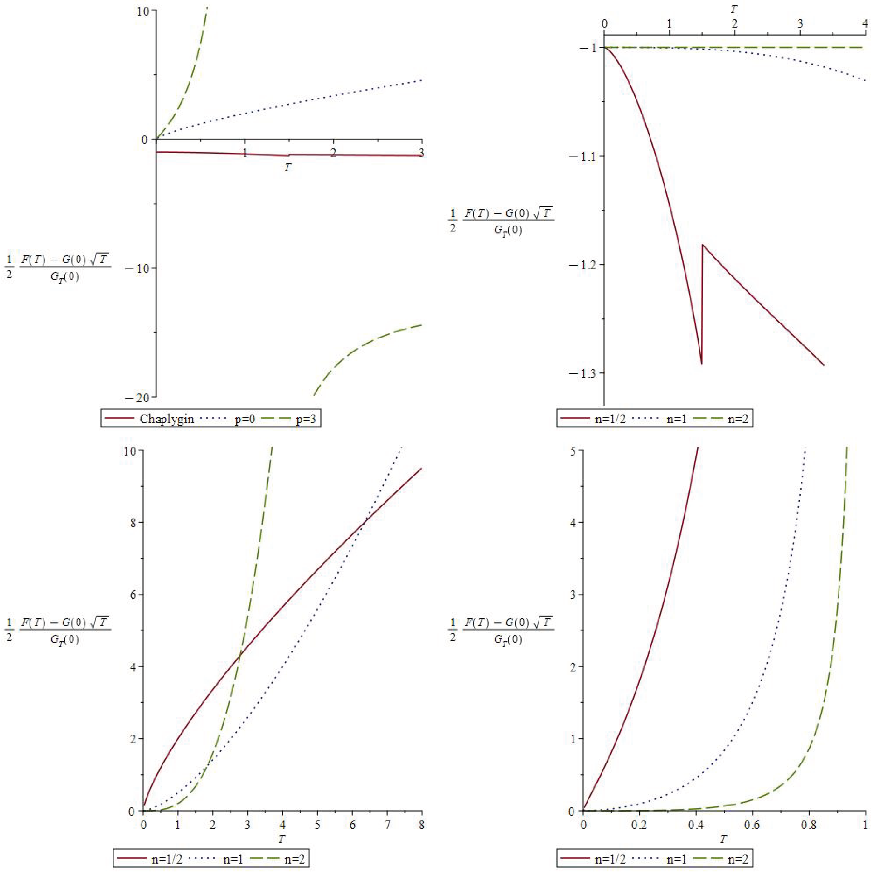

Table 1.
Values of function for the Equation (69) teleparallel flat polytropic solutions.
Table 1.
Values of function for the Equation (69) teleparallel flat polytropic solutions.
| p | |
| 0 limit | |
| 3 | |
Disclaimer/Publisher’s Note: The statements, opinions and data contained in all publications are solely those of the individual author(s) and contributor(s) and not of MDPI and/or the editor(s). MDPI and/or the editor(s) disclaim responsibility for any injury to people or property resulting from any ideas, methods, instructions or products referred to in the content. |
© 2025 by the authors. Licensee MDPI, Basel, Switzerland. This article is an open access article distributed under the terms and conditions of the Creative Commons Attribution (CC BY) license (http://creativecommons.org/licenses/by/4.0/).
Copyright: This open access article is published under a Creative Commons CC BY 4.0 license, which permit the free download, distribution, and reuse, provided that the author and preprint are cited in any reuse.


