
Submitted:
26 August 2025
Posted:
26 August 2025
You are already at the latest version
Abstract
Integrated hydrogen-electricity system(IHES) have gained widespread attention, yet distributed energy sources like photovoltaic(PV) and wind turbines(WT) power within them exhibit strong uncertainty and intermittency, posing key challenges of scheduling complexity and instability.Electricity price regulation, as a core mechanism in integrated IHES operation, can promote renewable energy absorption, optimize resource allocation, and enhance operational economy. However, uncertainties in IHES hinder accurate electricity price formulation, easily leading to delayed scheduling responses and increased cumulative operational costs.To address these issues, this paper establishes PEMEL and PEMFC models considering power-efficiency, incorporates their lifespan impacts into IHES scheduling, and integrates an electricity price regulation mechanism for energy imbalance. It constructs dynamic equations for the demand and response sides, scheduling electricity prices and IHES components via fuzzy weights and dynamic adjustment coefficients.Simulation results show that compared with fixed pricing, the proposed dynamic pricing reduces economic indices by an average of 15.3%, effectively alleviating energy imbalance and optimizing component energy supply. It also cuts PEMEL life attenuation by 21.59% and increases PEMFC utilization by 54.8%, providing theoretical and methodological support for efficient, stable IHES operation.
Keywords:
integrated hydrogen-electricity system
; day-ahead dispatch optimization
; electricity prices
; PEMEL/PEMFC lifespan degradation
1. Introduction
Energy generated from traditional resources such as fossil fuels causes air pollution in the short term. In the long run, it leads to an increase in atmospheric carbon dioxide, thereby triggering global warming [1]. Therefore, vigorously developing renewable energy and clean energy is one of the crucial approaches and goals for promoting the current energy transition and achieving global carbon neutrality [2]. In recent years, hydrogen has gradually attracted attention due to its unique advantages of zero carbon emissions, storability, transportability, and multi-energy conversion capabilities [3].The IHES, consisting of fuel cell(FC), hydrogen storage tank(HST), electrolyzer(EL), and supplementary batteries, can realize the functions of hydrogen production and storage, which is conducive to achieving zero emissions in the energy system. The energy supply of the IHES is highly dependent on distributed energy sources such as PV and wind power. However, the output of such energy sources is significantly affected by natural conditions, exhibiting characteristics of intermittency, volatility, and randomness [4].In addition, electric loads are also influenced by factors such as users’ living habits and seasonal climate, featuring large intraday peak-valley differences and sudden demand surges [5]. On the other hand, the deployment of new technologies such as electric vehicles(EVs) and hydrogen fuel cell vehicle(HFCVs) introduces greater complexity and uncertainty to load forecasting [6].The superposition of prediction deviations on both the energy supply and demand sides makes it difficult to achieve temporal matching in the multi-energy conversion chain of the IHES. Aspects such as the hydrogen production power of EL and the charging-discharging strategies of batteries all rely on accurate supply and demand forecasting schemes. Consequently, the decline in forecasting accuracy will make it difficult for the IHES to meet the preset economic dispatch targets [7].
Scholars have conducted extensive research on various issues in IHES; in terms of new energy forecasting, Emrani et al. [8] constructed a wind and PV power generation forecasting model based on on-site meteorological data, and by acquiring meteorological data, they predicted PV output power using a coupled model of solar irradiance and temperature, forecasted wind power output based on local wind speed piecewise functions and high wind speed characteristics, and verified the critical role of accurate forecasting in improving the economy and reliability of energy systems. Mellit et al. [9] took a specific PV system as the research object, investigated the forecasting performance of deep learning algorithms with different time steps and frameworks, validated the performance, training efficiency, and accuracy of the single Deep Learning Neural Network (DLNN) model, and demonstrated the application value of the single DLNN model in PV and wind power forecasting. Mirza et al. [10] proposed a hybrid deep learning model integrating ResNet, Inception modules, and bidirectional weighted LSTM/GRU for short-term and medium-term forecasting of wind and PV power based on wind and PV data from the State Grid Corporation of China and wind farm data from South Africa, and verified its accuracy and stability in wind and PV power forecasting. Sarmas et al. [11] constructed four basic LSTM models, used Support Vector Regression (SVR) to build a meta-learner that dynamically fuses the forecasting results of the basic models to adapt to the characteristics of different PV systems, and validated the model’s accuracy in PV power forecasting using power generation data from a PV plant in Portugal. After confirming that accurate renewable energy forecasting is a prerequisite for ensuring the efficient operation of IHES, the academic community has also carried out extensive basic and applied research on the structural design of the system itself to provide theoretical and experimental support for multi-energy conversion and supply-demand balance: Li et al. [12], in their research on IHES for net-zero energy buildings, configured a hydrogen energy subsystem consisting of an EL, a high-pressure HST, FC, and meanwhile realized a power coordination scheme using max-min game theory to achieve the goal of zero-carbon emission buildings; Shao et al. [13] proposed a structural framework for IHES that incorporates a hydrogen transportation subsystem, where hydrogen production stations powered by renewable energy produce and compress hydrogen, the hydrogen is then transported by trailers and finally stored in hydrogen refueling stations to supply hydrogen loads, filling the gap in the transportation aspect of IHES; Du et al. [14] proposed an off-grid-grid-connected hybrid design for IHES, which integrates a cooling-waste heat recovery module and auxiliary equipment, recovers waste heat generated during the operation of PEMEL and PEMFC through heat exchange plates, and optimizes the operating status of equipment via multiphase flow and thermal balance modeling to effectively reduce the frequency of PEMEL start-ups and shutdowns, thus enabling more efficient operational coordination of the hydrogen-electric coupling system. The aforementioned studies have explored IHES under different application scenarios from various perspectives, but few studies have considered the efficiency decline of EL and FC caused by their lifespan reduction—which in turn leads to decreased hydrogen production by EL and thus affects the operation of IHES [15]; additionally, the electric load exhibits significant peak-valley differences due to the randomness of EVs and HFCVs, making system dispatch optimization more challenging.
On the other hand, on the load side of IHES, with the popularization of new energy vehicles(NEVs), the strong uncertainties exist in users’ choices of charging/hydrogen refueling time and variations in travel routes, resulting in the load side exhibiting characteristics of large peak-valley differences and high volatility. Among existing studies on NEVs, for instance, Hussain et al. [16] proposed a local demand management model that integrates vehicle-to-vehicle (V2V) services with the welfare maximization-soft actor-critic (SAC) deep reinforcement learning approach. By means of dynamic pricing and charging-discharging optimization, and on the basis of considering the differences in EVs owners’ sensitivity to remaining battery capacity, battery degradation, and incentive prices, this model effectively alleviates the problem of distribution network transformer overload under high EV penetration rates, and realizes the coordinated optimization of owners’ welfare and power grid security. Eghbali et al. [17] put forward a scenario-based stochastic model; by fitting probability distribution functions for three types of uncertain parameters of NEVs, namely arrival time, departure time, and driving distance, and simultaneously combining with demand response programs, this model achieves the optimal dispatch of IHESs containing multiple energy sources and multiple ESS under the objective of minimizing the total system cost. Habib et al. [18] proposed a three-stage stochastic optimization structure, which generates parameter scenarios based on the normal distribution to address the uncertainty of NEVs; by combining vehicle-to-grid (V2G) technology, demand response, and energy storage, this structure realizes the optimal operation of a distribution system with four IHESs, thereby reducing costs and improving system performance. Wu et al. [19] proposed a two-layer model predictive control strategy, which samples the EV connection time and initial SOC, incorporates uncertainty sampling for extreme scenarios, and combines with EV arrival feedback to handle the uncertainty of EVs. This strategy optimizes the charging and discharging processes to reduce prediction errors and minimize the power exchange between the IHES and the main grid.
Given the aforementioned characteristics of volatility and randomness in source-load forecasting, researchers have conducted extensive studies on the dispatch optimization of IHES to improve the economic efficiency and stability of IHES. For example, Dong et al. [20] focused on the dispatch optimization of IHES, with hydrogen-water hybrid energy storage as the core. They adopted scenario-based algorithms to handle uncertainties and mixed-integer programming to clarify the relationships among multiple energy sources; this deterministic dispatch approach effectively reduced operating costs and increased the utilization rate of renewable energy. Zheng et al. [21] addressed the dispatch of biomass-integrated IHES, using Monte Carlo simulation to handle source-load uncertainties such as electric load and photovoltaic output. Combined with load shifting algorithm optimization, and under the consideration of time-of-use electricity prices and demand response, their work effectively mitigated the impact of source-load uncertainties on dispatch. For the hydrogen-electric hybrid energy storage system in IHESs with wind and photovoltaic generation, Li et al. [22] constructed a distributionally ambiguous set based on the Wasserstein distance, and applied distributed robust optimization to handle the source-load uncertainties of wind and photovoltaic output. They established a capacity optimization model targeting system economy and reliability, realizing the coordinated configuration of hydrogen and electric energy storage. Dong et al. [23] focused on the dispatch optimization of isolated hydrogen IHES.First, they used a bidirectional LSTM-CNN model to predict wind and photovoltaic output as well as load, thereby reducing source-load forecasting errors; then, they combined Monte Carlo simulation to generate stochastic scenarios for quantifying source-load uncertainties; finally, they applied deep reinforcement learning to solve the stochastic optimization dispatch problem involving energy storage capacity degradation, achieving the minimization of the IHES life-cycle cost. For hybrid IHES with green hydrogen production, Kim et al. [24] constructed a multi-period, multi-time-scale stochastic optimization model. They used Markov decision processes combined with deep Q-networks to handle source-load uncertainties, and simultaneously employed Monte Carlo simulation to generate stochastic scenarios of wind and photovoltaic output and load, realizing the coordinated optimization of capacity investment and energy management. Wu et al. [25] targeted IHES with hydrogen fuel cell stations, adopting a data-driven chance-constrained approach to handle the source-load uncertainties of wind and photovoltaic output as well as electric-hydrogen load, while using distributed robust optimization to address electricity price uncertainties. Through converting the problem into a mixed-integer linear programming via an affine strategy, they achieved system dispatch optimization. Based on the above studies, it can be concluded that existing works have effectively handled source-load uncertainties through various methods such as scenario-based algorithms, Monte Carlo simulation, and distributed robust optimization, providing technical support for the dispatch optimization of IHES [26,27]. However, most of these studies take fixed time-of-use electricity prices or static electricity prices as constraints, and have not fully explored the core value of dynamic electricity price regulation in addressing source-load fluctuations and optimizing dispatch strategies [28].
Compared with traditional IHES based on EL/HST/FC, research considering HFCVs and hydrogen refueling stations remains relatively limited. References [13,18,25] have discussed and explored this topic, but they do not account for the lifespan impact of two critical components: PEMEL and PEMFC. Furthermore, in most studies, the randomness of NEVs and their characteristic of significant peak-valley differences are often overlooked, which may lead to misjudgments regarding the hydrogen production capacity of PEMEL and the hydrogen absorption capacity of new energy sources. In addition, electricity prices—an important means of regulating demand response—are usually neglected. Therefore, this paper proposes a day-ahead dispatch optimization scheme for IHES that considers the impact of electricity prices on demand response. This scheme incorporates the lifespan-efficiency effects of PEMFC and PEMEL, and predicts the load side based on the probability density function of vehicle owners’ behaviors. To summarize, the contributions of this paper are as follows: (1) A lifespan-efficiency model for PEMFC and PEMEL is established, which accounts for the impact of PEMFC and PEMEL lifespans on efficiency. Additionally, lifespan degradation models for PEMFC and PEMEL under different operating conditions are developed to enhance the accuracy and reliability of hydrogen prediction in IHES. (2) A load forecasting model for NEVs is constructed. Based on the probability density function of vehicle owners’ behaviors, Monte Carlo simulation is used to predict daily driving mileage, charging start time, and required electricity demand of NEVs, and finally load curves on the load side under different scenarios are obtained. (3) A dynamic pricing strategy considering demand response is proposed. First, dynamic balance equations for the power supply side and load side are established; the system is then divided into several different operating states based on the energy imbalance between the power supply side and load side. Subsystems are weighted and combined using fuzzy weights, and linear matrix inequality (LMI) equations are applied to enable the system to meet preset performance requirements.
The remaining parts of this paper are organized as follows: Section 2 presents detailed mathematical models; Section 3 introduces the electricity pricing strategy and the algorithm for mathematical constraints; case studies are illustrated in Section 4; and finally, conclusions are given in Section 5.
2. System Configuration and Mathematical Model
As shown in Figure 1, this section introduces an integrated hydrogen-electric coupling system referenced from the Ningbo Hydrogen-Electric Coupled DC IHES Demonstration Project in China. In the proposed system, PV panels and wind turbine systems generate electricity to supply power to IHES loads and NEVs. The system stores surplus energy during periods of high renewable energy generation and compensates for energy shortages through energy storage devices when renewable energy generation is low. The IHES includes the EVs and HFCVs on the load side. On one hand, PEMEL produce hydrogen by electrolyzing water using surplus electricity, and the hydrogen is then stored in hydrogen storage tanks to supply HFCVs. On the other hand, the hydrogen in the storage tanks can be further used by PEMFC to generate additional electricity for the system. In addition, lithium-ion batteries are utilized as energy storage devices in this paper, ensuring greater flexibility for power applications. The main function of the main grid is to fill the energy gap, thereby maintaining the energy balance between the supply side and the demand side.
2.1. Mathematical Modeling
To quantitatively characterize the operational mechanisms of each component, clarify the coupling relationships between different energy flows, and provide a reliable mathematical basis for subsequent day-ahead dispatch optimization, this section will introduce the mathematical models of each component. These models are constructed to address the core challenges of the integrated hydrogen-electric coupling system, including the nonlinearity of energy conversion, the coupling constraints between power and hydrogen networks, and the impact of device degradation on system efficiency
2.1.1. Photovoltaic Panels (PV)
The main power generation unit in this system relies on PV technology, where PV panels convert solar radiation into electrical energy. PV power generation devices form a power generation array by connecting multiple PV cells in series and parallel. The corresponding power generation mainly depends on solar irradiance, PV cell temperature, and power generation efficiency. It omits the analytical modeling of complex internal physical processes such as carrier transport and PN junction characteristics in traditional models, and accurately reflects the external characteristics of component power output through the calibration of efficiency and photovoltaic radiation. This approach can simplify the model to a certain extent while still capturing the essential characteristics of photovoltaic power generation. Its mathematical model is as follows [20]:
denotes the effective radiation area on the PV panel; N is the number of PV cells; and indicates the solar irradiance value. Among them, is related to the radiation intensity and ambient temperature, and its specific expression is shown as follows:
Where denotes the efficiency of the solar photovoltaic panel under reference conditions, represents the temperature coefficient, stands for the operating cell temperature under standard test conditions, and is the reference temperature of the solar photovoltaic panel [30].
2.1.2. Wind Turbine Systems (WT)
In the WT system, the WT drives a permanent magnet synchronous generator to generate electricity, and its output power is converted into direct current through a rectifier and a boost converter for energy supply. The rectifier and boost converter ensure that the power quality meets the requirements of the IHES DC bus. The losses in the rectifier and converter are neglected herein. Therefore, the DC output of the wind system is equal to the wind energy captured by the wind blades, and its specific modeling is as follows [31]:
where denotes the air density, represents the wind speed, is the radius of the rotor blades, and the rotor efficiency is a function of the tip speed ratio and the pitch angle.
1.1.3. Proton Exchange Membrane Electrolyzer(PEMEL)
When the power generated by renewable energy exceeds the demand of electrical loads, the surplus electricity will be supplied to the PEMEL, which consumes electricity and converts water into hydrogen and oxygen. In this system, a PEMEL is used, and its mathematical model is as follows [32]:
where is the open-circuit voltage, is the activation potential, is the concentration overpotential, and is the ohmic overpotential, which are given by the following equations:
In the above equations, , is the gas constant, is the Faraday constant, and is the stack temperature of the PEMEL. Here, is the operating current, where and represent the current density and the cross-sectional area of the electrode, respectively [33]. In addition, and denote the exchange current densities in the anode and cathode, respectively; is the ohmic resistance of the PEMEL; and is the defined maximum current density. The amount of hydrogen produced by the PEMEL per unit time is as follows:
The efficiency of the PEMEL is the ratio between the energy of hydrogen produced per unit time and the input power [34]. Under the conditions where the basic parameters, operating temperature, and pressure of the PEMEL are determined, the mass of hydrogen produced by the PEMEL per unit time can be determined, and thus the efficiency of the PEMEL can be calculated as follows:
In the equation, represents the efficiency of the PEMEL, is the power of hydrogen produced by the PEMEL, is the input power of the PEMEL, and and denote the higher heating value of hydrogen and the molar volume of hydrogen, respectively.
2.1.4. Proton Exchange Membrane Fuel Cell (PEMFC)
As described in the structure of the aforementioned IHES, when the power generated by the PV and WT is insufficient, the PEMFC will consume the hydrogen in the HST to provide electrical energy to the load. The system in this paper uses a PEMFC. The mathematical model of the PEMFC is as follows [35,36,37]:
Similar to the PEMEL, where is the open-circuit voltage, is the activation potential, is the concentration overpotential, and is the ohmic overpotential, which are given by the following equations:
In the above equations, is the Gibbs free energy change, is the entropy change, is the cell current, is the operating temperature of the cell, and and are empirical coefficients obtained from experimental fitting. Similar to the modeling of the PEMEL, the gas pressures of hydrogen used in the PEMFC, and , are calculated through balance equations, and is a fixed parameter of the PEMFC [38]. Similarly, the rate of hydrogen consumption per unit time by the PEMFC can be obtained from the following equation:
Similar to the PEMEL, the efficiency of the PEMFC is the ratio of the output power to the energy of the consumed hydrogen [39]:
In the equation, represents the efficiency of the PEMFC, is the power generated by the PEMFC from hydrogen, is the input power of the PEMFC, and and denote the higher heating value of hydrogen and the molar volume of hydrogen, respectively.
Similarly, in References [39,40],the efficiency-power relationships of PEMFC and PEMEL are introduced, which are similar to those discussed in this paper.As shown in Figure 2 is the efficiency-power curve of the PEMEL and the PEMFC. It can be seen from Figure 2 that as the input power increases, the efficiency of PEMEL improves rapidly, reaching a maximum efficiency of approximately 85% at 25% of the rated power, and then gradually decreases as the power of the PEMEL increases, with the efficiency being only about 67.8% at the rated power. However, the hydrogen production amount is the largest at this point. The gradual decrease in the efficiency of PEMEL can be attributed to the ohmic resistance in PEMEL and the reduction in current efficiency.
Moreover, as shown in Figure 2b is the efficiency-power curve of the PEMFC, whose general shape is similar to that of PEMEL. However, due to the accumulation of multiple losses in its “electricity-chemistry-electricity” reverse process, the efficiency of the fuel cell is lower than that of PEMEL. As can be seen from the figure, the efficiency reaches a maximum value of approximately 50.37% at 20% of the rated power, and only about 35.07% at the rated power. Therefore, it can be seen that when the power generated by WT and PV systems is unstable, it will cause significant fluctuations in the efficiency of the PEMFC and PEMEL. It is necessary to consider the efficiency of the PEMFC and PEMEL during IHES dispatching, and compensate for the efficiency of PEMEL and the PEMFC through the ESS.
2.1.5. Degradation Models of PEMFC and PEMEL
In references [41,42,43], the principles of degradation mechanisms for PEMFC and PEMEL are introduced. The degradation principles of the two are similar, mainly stemming from the chemical degradation of membrane materials, the dissolution and agglomeration of catalyst layers, and the mechanical failure of the electrode-membrane interface under humidity and thermal cycles. Therefore, in this paper, it is considered to establish the same degradation modeling method for both.
The continuous operation of PEMFC and PEMEL will cause degradation of internal components, leading to lifespan attenuation of PEMEL and PEMFC. Moreover, the lifespan attenuation of PEMFC and PEMEL varies under different operating conditions. When PEMEL and PEMEL operate stably, there will be a certain amount of lifespan attenuation. When fluctuations occur in WT and PV power generation, the input power of PEMEL will fluctuate frequently and start/stop frequently, accelerating lifespan attenuation. In addition, when the output exceeds the rated power, the lifespan attenuation of PEMFC and PEMEL will also accelerate. Therefore, in this paper, four different operating conditions of PEMFC and PEMEL are set to measure the lifespan attenuation under different conditions, namely low-power operation, high-power operation, fluctuating operation, and start-stop operation. Each operating condition has a different attenuation coefficient. Under low-power and high-power operating conditions, the attenuation coefficients are lower, so the lifespan attenuation is relatively slow; under fluctuating operating conditions, the attenuation coefficients are higher, and the greater the fluctuation, the faster the lifespan attenuation; frequent start-stops have the greatest impact on the lifespan of PEMFC and PEMEL.
Taking the PEMEL as an example, the lifespan models established under different operating conditions are as follows:
In the equation, respectively represent the lifespan attenuation amounts of the PEMEL under the four different operating conditions, and respectively denote the operating states of the PEMEL under the four different conditions: low-power operation, high-power operation, energy fluctuation, and frequent start-stops. represents the attenuation coefficient under different operating conditions, with values taken as , , and here. is the rated power of the PEMEL; is the rated attenuation coefficient of the PEMEL; and are the total efficiency attenuation amount and equivalent lifespan attenuation amount of the PEMEL within a scheduling cycle, respectively; and are the rated efficiency and limit efficiency of the PEMEL, respectively; is the rated lifespan of the PEMEL.
and in (6) and (10) vary according to the attenuation given by the following equation:
2.1.6. Energy Storage Systems (ESS)
In this paper, lithium battery modules and hydrogen storage tanks are considered as the energy storage system, where the hydrogen produced by the PEMEL is charged into the hydrogen storage tanks. The hydrogen storage tanks are not only responsible for refueling HFCVs but also can supply hydrogen to PEMFC for energy provision; lithium batteries can ensure the stability of the system, generate electricity when the power generated by distributed energy sources is insufficient, store energy when the generated power is sufficient, and can provide support for peak shaving and valley filling of electrical loads. The mathematical modeling of the energy storage system in this paper is shown in (15) and (16) as follows:
In the equation, and are the charging and discharging powers of the lithium battery at time t, respectively; and denote the charging and discharging efficiencies of the lithium battery, respectively; represents the battery capacity; is a binary variable controlling the charging and discharging of the lithium battery, where indicates the discharging state and indicates the charging state. Similar to the state of charge of the lithium battery, the hydrogen storage state of the hydrogen storage tank is shown in (16), where and are the actual operating electrical powers of the PEMEL and the PEMFC, respectively; is the capacity of the hydrogen storage tank; is the required hydrogen refueling amount of the i-th HFCVs at time t; and represents a binary variable indicating whether the i-thvehicle needs refueling.
2.1.7. EVs and HFCVs
With the popularization of EVs in recent years, the large-scale integration of EVs will bring issues such as power fluctuations and grid overload to the IHES, and the uncertainty of EVs owners’ behaviors will also significantly affect the charging characteristics of EVs.In addition, the impact of random refueling loads from HFCVs on hydrogen refueling stations is similar to that of charging loads from EVs on charging stations [44].Therefore, it is quite necessary to implement reasonable scheduling and optimization strategies for EVs. Considering that HFCVs and EVs have similar characteristics, in this paper, probability distributions are used to model the start charging time and daily driving distance of EVs and HFCVs, as shown in the following equations:
Considering the daily driving distance of EVs, the SOC or SOH when arriving at the charging station/hydrogen refueling station can be expressed as follows:
Wherein, represents the battery capacity of the EVs or HFCVs, and denotes the energy consumption for the driving distance to the next charging station/hydrogen refueling station.
3. Optimization Strategies for Integrated Hydrogen-Electric System
Based on the aforementioned mathematical model, to address the problems of supply-demand imbalance, system instability, and inefficient demand response caused by the uncertainty of renewable energy output, this paper proposes a dispatch strategy for IHES based on fuzzy-weighted dynamic pricing [45]. The strategy operates as follows: first, the fuzzy weight method is used to decompose the system’s nonlinear characteristics into multi-state subsystems, and dynamic weights are assigned according to the system’s energy state to match real-time scenarios; second, the baseline electricity price is determined based on the subsystem state, and a price adjustment term is calculated by combining the energy imbalance value, enabling the electricity price to be linked to supply and demand to guide both the supply and load sides; finally, LMI equation is solved to design control gains, which satisfy the performance criteria, realize the coordinated dispatch of multi-energy components, balance economy and stability, and resolve supply-demand imbalance.
3.1. LSTM Projected Source-Load Side
In the context of formulating dynamic pricing strategies for the power market, accurately predicting the source—load side conditions is crucial. Dynamic pricing needs to adapt to real—time fluctuations in power generation and consumption, and precise source—load prediction provides the foundation for rational price adjustments. As illustrated in Figure 3, it presents the flowchart of the LSTM—based prediction for the source-load side data. The following LSTM—based process helps achieve this prediction. In data preprocessing, historical generation and load data undergo imputation, outlier removal, and normalization to refine it for analysis. Time-series samples are then constructed, and the dataset partitioned for LSTM training. Next, in LSTM, processed data passes through the forget gate, input gate, and cell status update. The output gate generates predictions, with loss calculation evaluating accuracy. This source-load prediction underpins dynamic pricing strategy formulation.
3.2. Dynamic Pricing Strategy
To achieve effective coordinated scheduling of multi-energy components in the hydrogen-electric coupling, it is essential to establish a dynamic pricing mechanism that can accurately reflect the real-time supply-demand relationship and guide the operation of both supply and demand sides [45]. This dynamic pricing strategy serves as a core signal bridge.on one hand, it quantifies the impact of renewable energy output uncertainty on the system’s energy balance; on the other hand, it regulates the power generation behavior of supply-side adjustable devices and the energy consumption behavior of demand-side loads through price signals, thereby mitigating supply-demand imbalances and improving system stability and economic efficiency. To lay a rigorous mathematical foundation for this dynamic pricing strategy, it is first necessary to construct dynamic equations that characterize the response laws of the supply and demand sides to price changes. These equations will explicitly describe how the supply-side power generation and demand-side energy consumption adjust with real-time electricity prices, while incorporating factors such as renewable energy uncertainty, device operating constraints, and user demand elasticity. Such modeling ensures that the subsequent pricing strategy is not only theoretically sound but also capable of simulating and guiding the actual operation of the IHES. Next, the dynamic equations for the supply side and demand side in the dynamic pricing strategy will be introduced to enable the scheduling of various components of the IHES through electricity prices. Dynamic equation of the supply side:
Wherein, represents the total power generation of the IHES system at time k+1; denotes the power generation response time constant; is the real-time electricity price at time k; stands for fixed costs such as equipment depreciation and maintenance; reflects the impact of uncertainties like the output volatility of renewable energy; is the power generation elasticity coefficient, which reflects the sensitivity of power generation to electricity prices—when , a rise in electricity prices will prompt an increase in the power generation of adjustable power generation equipment; and represents the energy imbalance.Dynamic equation of the demand side:
In a similar manner to the dynamic equation of the supply side, represents the electricity demand at time k+1; denotes the demand response time constant; is the marginal benefit of the demand side, which reflects customers’ basic willingness for electricity demand; reflects the volatility impact caused by uncertainties; and is the demand elasticity coefficient, which indicates the sensitivity of the demand side to changes in electricity prices. Dynamic equation of energy imbalance:
Wherein, represents the power generated by renewable energy; denotes the energy imbalance at time k, which is a core signal triggering changes in electricity prices; and is a discrete fixed time step. Therefore, based on the above equations, the overall dynamic state equation of the IHES can be expressed as the following state-space system:
Wherein, is the system matrix, is the disturbance input matrix, is the constant vector, and is the input matrix of price signals. Thus, the system can be characterized in the following form:
Dynamic pricing strategy: firstly, in order to handle the nonlinear dynamic system, the system is decomposed into several subsystems through the following equations, where each subsystem corresponds to a different operating state (such as high power generation, low demand, or equilibrium state, etc.):
Wherein, is the fuzzy weight of the current state, which is dynamically assigned according to the current membership function , and is the approximation error, as shown in the following formula:
Similarly, the electricity price regulation strategy can be obtained by the weighted combination of each subsystem and the supply-demand adjustment term, as follows:
Wherein, is the system benchmark price, which is generated based on the operating state of each subsystem; is the electricity price adjustment term derived from the power imbalance value, determining the fluctuation range of electricity prices. By integrating equations (28) and (30) into equation (29), the following formula can be obtained:
Wherein, , , . To address the uncertainty in renewable energy generation, the control gains are designed via linear matrix inequalities, while ensuring the satisfaction of the performance criteria :
Where , is the fluctuation attenuation level coefficient; and are used to prevent significant fluctuations in pricing. To satisfy in equation (31), we can solve the LMI equation:
3.2. Day-Ahead Scheduling Optimization and Constraints
Day-ahead scheduling is based on historical data to predict various load demands and renewable energy generation for the next day. Combined with historical variable electricity prices and the constraints of various devices, it takes the total economic cost as the objective function to formulate a full-day advance scheduling plan. Therefore, in the day-ahead scheduling stage, predicting various load demands and renewable energy generation is a key step. This section will introduce the prediction methods, objective function, and various constraints used.
3.2.1. Objective Function for Day-Ahead Scheduling
Equation (34) presents the objective function of day-ahead scheduling aimed at maximizing revenue, which includes the operating costs of the energy storage system and , the cost of purchasing electricity from the grid , the operating costs of renewable energy ( and ), and the operating costs of the PEMEL and PEMFC ( and ). Among them, and respectively represent the configuration replacement costs of the PEMEL and PEMFC.
2.2.2. Electrical Power and Hydrogen Power Balance Constraints
The electrical power balance of the system is shown in (35), where the distributed energy sources operating in the IHES must be able to meet the load demands within the IHES. When the energy supplied by distributed energy sources is insufficient, external power grids will be used for energy supply to ensure that the load demands are met. The hydrogen power balance is shown in (36), which takes into account the hydrogen refueling amount of hydrogen fuel cell vehicles at time t.
where is the electrical power exchanged with the external power grid at time t; and are the power generation of wind and photovoltaic at time t;is the predicted charging power of EVs obtained by the Monte Carlo simulation method in Section 2; is the electrical power of the basic load in the IHES; and are the discharging or charging power of the battery; and are the operating electrical power of the PEMFC and PEMEL. In (36), where and represent the amount of hydrogen output or input by the PEMEL and PEMFC at time t. Herein, is positive when the hydrogen storage tank releases hydrogen, and negative when the hydrogen storage tank stores hydrogen; is the hydrogen refueling amount of HFCVs at time t.
3.2.3. ESS Constraints
Equations (37) and (38) represent the charging and discharging power limits of the battery, respectively. The binary variable indicates the charging/discharging state of the battery at time t. Equation (39) represents the SOC limit of the energy storage.
3.2.4. Hydrogen Energy Constraints
Equations (40) and (41) respectively restrict the electrical power of the PEMEL and the PEMFC. The binary variable represents the hydrogen storage state of the HESS at time t. Equation (42) represents the hydrogen storage state constraint of the hydrogen storage tank. Since the hydrogen in the storage tank should be available for HFCVs, the SOH constraint of the hydrogen in the storage tank must be maintained above 20%.
3.2.5. Distributed Energy Resources and Grid Power Constraints
Equations (44) and (45) respectively restrict the maximum power of wind power generation and photovoltaic power generation, while equation (43) limits the maximum electrical power exchanged between the IHES and the power grid.
3.2.6. External Power Grid Constraints
In the equation, and denote the electrical power purchased by the IHES from the external power grid and the electrical power sold to the external power grid, respectively. and are logical variables that prevent the IHES from simultaneously purchasing and selling electricity from/to the external power grid
3.2.7. System Flow Chart
Figure 4 systematically expounds the method of wind-solar load data prediction and dynamic electricity price strategy scheduling based on LSTM. Firstly, historical data of wind, PV, and load are collected, and a system model is constructed, covering component models such as PV, WT, BAT, HST, PEMEL, PEMFC, as well as models of EVs and HFCVs. Meanwhile, constraints such as energy balance, system components, energy storage, and the main grid are considered, and mathematical modeling of PEMEL and PEMFC is carried out, including polarization curves and system efficiency curves. In the Methodological section, the wind-solar load data are first preprocessed, the data set is divided, and the LSTM model is constructed and trained to output the prediction results. Then, based on the predicted data, dynamic equations for the power supply side and the demand side are constructed to judge the energy imbalance situation. Furthermore, electricity prices are adjusted and dispatchable units (PEMFC, BAT) are scheduled, and finally, the system scheduling results are output. The entire process is closely connected, providing an effective technical path for the optimal operation of wind-solar-storage systems.
4. Discussion
In this section, a case study is conducted on the virtual IHES described in Figure 1 to verify the feasibility of the proposed method. The simulation verification is performed in Matlab using the Gurobi solver on a Windows PC desktop, which is equipped with an Intel Core i7-9750H CPU and 16GB RAM. The system parameters and simulation parameters are provided in the Appendix A.
4.1. Source-Load Side Electricity Prediction
In this section, the historical short-term forecast data and historical data of photovoltaic and wind power output in a certain area of Ningbo are selected as the dataset, and the conventional deep learning model LSTM is used to predict their short-term power generation and electricity consumption. The data spans from 1 January 2019 to 31 December 2019. Due to their variable nature, the sampling frequency for wind and photovoltaic power is set to 15 minutes, while the load varies to a smaller extent in a certain period, so the sampling frequency is set to 1 hour. Both the predicted and measured data sequences have a length of 35040. After the data is processed, the training set and test set are divided in a ratio of 0.8 to 0.2. Figure 5 shows the monthly predicted data of photovoltaic power, wind power, and load respectively.
The Figure 6 illustrate the prediction errors of a certain method for PV, WT and Load power. For PV power prediction, the coefficient of determination reaches 0.99, with a mean absolute error (MAE) of 1.6 and a root mean square error (RMSE) of 3.17, indicating that the predicted values are in good agreement with the actual values, and the prediction accuracy is relatively high. In terms of WT power prediction, the is 0.99, the MAE is 2.76, and the RMSE is 4.8, which also shows that the prediction results are highly consistent with the actual situation. For load power prediction, the is 0.97, the MAE is 4.05, and the RMAE is 5.92, reflecting a relatively ideal prediction effect. Overall, this method has high accuracy and reliability in predicting wind, solar, and load power, and can provide strong support for the energy scheduling of IHES.
4.2. Monte Carlo Simulation of Load for EVs/HFCVs
As shown in Figure 6, it is the probability density function of the random behavior of vehicle owners based on historical data. It is assumed that there are 20 new EVs and 10 HFCVs in this IHES. As shown in Figure 7a, it is the arrival time of electric vehicles and hydrogen fuel cell vehicles at charging stations/hydrogen refueling stations. It can be seen that there are usually more vehicles arriving at 18:00 p.m., and the charging peak usually occurs at this time. As shown in Figure 7b, it is the probability density function of the average daily driving mileage of vehicles. As shown in Figure 8, it is the daily demand load curve of EVs and HFCVs obtained by the Monte Carlo method under high load and low load conditions.
After completing the prediction of wind and PV power output, base load, and the load curves of EVs/HFCVs based on the LSTM model, it is necessary to classify the operating scenarios according to the daily total power generation to further clarify the system scheduling direction under different supply-demand matching states. Specifically, the daily total wind-PV power generation is taken as the core basis for classification. With reference to the distribution characteristics of historical wind-PV power generation data over 6-12 months, the 60th percentile is adopted to set the threshold for high wind-PV power generation. A day is classified as a “high-power generation day” when its daily power generation exceeds this 60th percentile threshold; similarly, a day is identified as a “high-load day” when its daily load surpasses the 60th percentile threshold of load. This scenario classification enables targeted analysis of the scheduling effects of the dynamic pricing strategy under different supply-demand backgrounds and provides clear scenario boundaries for the subsequent verification of optimized system operation. The specific scenario classification is presented in Table 1.

| Scenario Category | Judgment of Daily Total Power Generation | Judgment of Daily Total Load | Examples |
|---|---|---|---|
| High-Power Generation & High-Load Day | ≥ 60% (historical daily power generation data) | ≥ 60% (historical daily load data) | Sunny days+working days |
| Low-Power Generation & High-Load Day | < 60% | < 60% | Cloudy days+summer working days |
| Low-Power Generation & High-Load Day | < 60% | ≥ 60% | Rainy days+holidays |
4.3. Prediction Results and Electricity Price Regulation Effects
Figure 9a depicts the 24-hour daily variation characteristics of photovoltaic output, wind power output, and net load under high wind-solar generation and high load conditions. Wind power exhibits instability and strong time-variability with multiple daily peaks and troughs; photovoltaic output follows a typical daytime pattern—negligible from 0:00-4:00, rising slowly from 5:00, and peaking between 10:00-12:00. Load power remains generally high with minor fluctuations, being higher in the morning and evening (peak at 18:00, trough at 14:00). The load curve’s double-peak feature is closely linked to residential and industrial electricity consumption habits.
Similar to Figure 9a, Figure 9b shows daily variations under low wind-solar generation and low load conditions, where low wind power output fails to meet load demand. Overall, significant grid electricity purchases are required during early mornings or periods of insufficient photovoltaic output to meet demand. Here, dynamic pricing effectively incentivizes users to adjust consumption by reflecting real-time grid supply-demand tensions, reducing peak demand and easing purchase pressure.
Compared to fixed pricing, dynamic pricing prompts users to reduce consumption during high-price periods (avoiding costs from concentrated purchases), enhances system economic efficiency and operational safety, optimizes grid resource allocation, lowers reserve capacity needs, and improves overall energy utilization—ultimately reducing both purchase costs and operational risks.
Figure 10 presents the scheduling status of load levels and dispatchable units under the dynamic pricing strategy and the constant electricity price strategy. Through comparative analysis of Figure 10a,b, it can be seen that the dynamic pricing strategy shows significant differences in the scheduling of loads and dispatchable units. Taking 11:00 as an example, compared with the constant pricing strategy, the load at this time increases by 4.2%. This phenomenon indicates that in the case of excess wind and solar energy, the dynamic pricing strategy can effectively stimulate load growth by means of reducing electricity prices, thereby achieving more energy consumption. When the power generation of wind and solar energy decreases sharply, for example, at 1:00 at night, the photovoltaic power generation is scarce, and wind power generation is also difficult to meet the load demand. The dynamic pricing strategy successfully reduces the load by increasing the electricity price. At the same time, dispatching dispatchable energy sources such as proton exchange membrane fuel cells and lithium batteries not only reduces the dependence of the IHES on the main grid, but also optimizes the economy of system operation. In the working conditions corresponding to (e) and (f), since the power generation of wind and solar energy is continuously in a scarce state, and the energy reserves of the energy storage system will also be gradually exhausted. At this time, the dynamic pricing strategy continuously suppresses the load demand by increasing the electricity price according to the characteristics of energy imbalance in the IHES. This is because even during periods with relatively sufficient wind and solar power generation such as during the day, there is still an energy imbalance between the power supply side and the demand side. Compared with the constant electricity price strategy, the dynamic pricing strategy reduces the 24-hour total load by 16.2%, which fully verifies the effectiveness of the dynamic pricing strategy under this working condition.
4.4. Operation and Degradation of PEMEL and PEMFC
Figure 11 shows the relevant scheduling of hydrogen component operation under different scenarios. From the perspective of the service life of PEMEL and PEMFC, dynamic pricing guides the power output of PEMEL and PEMFC to closely match the peak periods of new energy generation through real-time price signals, which improves the load utilization rate and operational stability of the equipment, and avoids frequent start-stop of PEMEL and PEMFC, thereby extending their service life. Secondly, this strategy effectively promotes the local consumption of volatile new energy such as WT power and PV power, reduces the curtailment of wind and PV power, and improves the utilization efficiency of renewable energy. Finally, from the economic perspective, PEMEL operate continuously during low electricity price periods to ensure sufficient hydrogen in the storage tanks, and PEMFC operate during high electricity price periods to provide necessary electrical energy supplement. By optimizing load distribution and energy conversion, dynamic pricing significantly improves the economic efficiency of the system, reduces operating costs and increases overall revenue.
Figure 12 presents the lifespan degradation of PEMEL and PEMFC across cases. As shown in Figure (a), PEMEL exhibit a significantly lower average degradation rate than in Figure 12b, attributed to their continuous operation during sufficient wind-solar generation. This avoids frequent start-stops, keeps equipment in optimal operating ranges, and reduces wear from high loads or cycling.
In contrast, PEMFC show slightly higher degradation under dynamic pricing than fixed pricing. This arises because PEMFC must operate longer during early mornings and nights (when PV output is low) to sustain essential loads. Under fixed pricing, ineffective scheduling leads to brief, intermittent operation, causing greater degradation from frequent start-stops—whereas dynamic pricing yields higher overall IHES benefits despite this.
For system flexibility, dynamic pricing allows mode adjustments: in Case 3 (low renewables, high load), increasing PEMFC output meets demand. Though this raises fuel cell degradation, it enhances system responsiveness and slightly boosts overall revenue. Compared to fixed pricing, dynamic pricing also aligns user behavior with price signals, reducing transferable loads, peak-valley gaps, and unnecessary fluctuations—validating its effectiveness.
4.5. Day-Ahead Scheduling Results
Figure 13 compares day-ahead scheduling under dynamic and fixed pricing across three scenarios. In Scenario I, as photovoltaic generation is unavailable at night, substantial grid electricity must be purchased between 0:00-6:00 and 20:00-24:00 to maintain essential loads. Figure 8a,b show optimized scheduling for Case I under the two pricing strategies, with regular load variations across periods. For example, prices rise between 1:00-4:00 under dynamic pricing, reducing demand; between 10:00-12:00, higher renewable output lowers prices, boosting load response while energy storage charges for use during shortfalls. Fixed pricing, by contrast, fails to signal real-time supply-demand, leaving user behavior unconstrained—causing large, irregular load fluctuations that hinder system stability and resource allocation. Overall, dynamic pricing aids peak shaving and valley filling, shifting demand to stabilize IHES operation.
Figure 13c,d show Case II scheduling. Dynamic pricing curbs peak loads via higher prices—e.g., 17:00 load drops 13.2% vs. fixed pricing, as users reduce or shift demand. It also shifts load to low-price periods with high renewables, such as a 22.74% load increase at 6:00, easing peak grid pressure. Combined with energy storage, this enables dual optimization of peak shaving and renewable utilization, unlike rigid user behavior under fixed pricing, which struggles with renewable output fluctuations.
Similarly, Case III results (Figure 13e,f) show dynamic pricing slightly higher under extreme conditions, as insufficient renewables require price hikes to suppress demand. It sets high prices at 7:00 (peak) to cut purchases or boost storage discharge, and low prices at 1:00 (off-peak) to encourage buying/charging. This reduces total energy costs by 5.19% vs. fixed pricing. Dynamic pricing also smooths load curves by shifting demand to off-peak periods, cutting daily peak load by 17.4% and easing grid pressure. Lower prices between 12:00-16:00 further incentivize charging and storage.
4.6. IHES Operation Cost Results
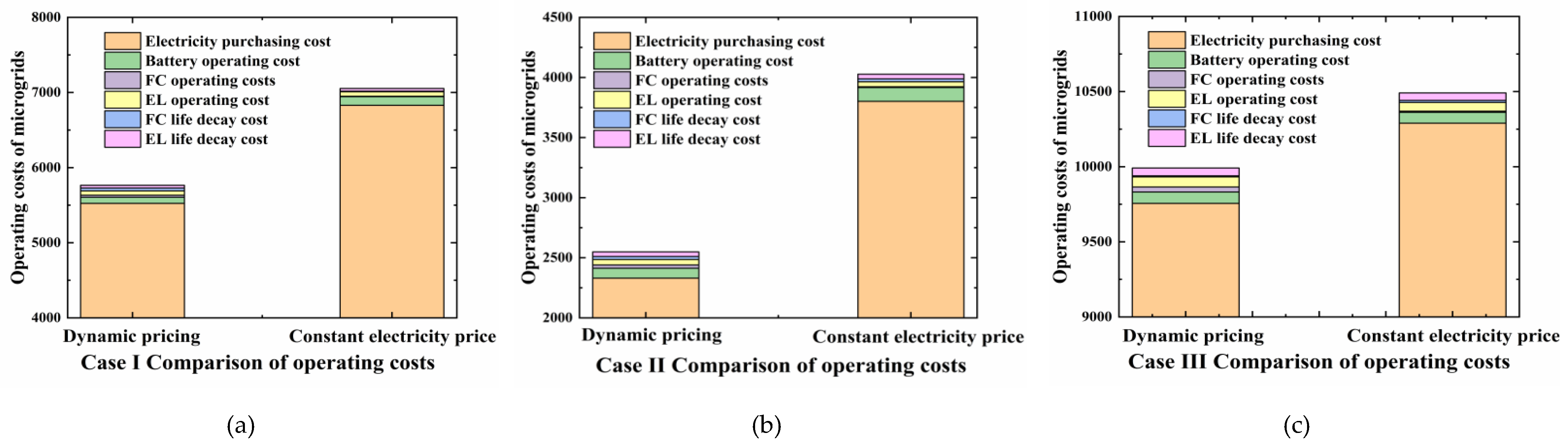
Figure 14 shows the costs of the IHES under the dynamic pricing strategy and fixed pricing strategy. It can be seen from the figure that under most conditions, the output of distributed energy is insufficient to meet the demand of essential loads, so it is necessary to purchase electricity from the main grid, making the electricity purchase cost account for a large proportion of the operation cost. In addition, the operation cost rises sharply under extreme conditions, Case III. This is because insufficient wind and solar power generation under such conditions necessitates purchasing electricity from the main grid. However, the cost of the dynamic pricing strategy is about 5.123% lower than that of the fixed pricing strategy. Moreover, under various conditions, the dynamic pricing strategy can adjust the operation of each component to ensure they run within appropriate ranges, thereby reducing the IHES operation cost. Particularly in Case II, with sufficient wind and solar power generation, there is a larger adjustable range. As indicated in Figure 13c,d, the dynamic pricing strategy can store electricity when wind and solar generation is abundant for use in periods of insufficient generation (such as morning and evening), which helps reduce costs in such scenarios. Therefore, it is evident that the dynamic pricing strategy can reduce costs to a certain extent compared with the fixed pricing strategy across different scenarios.
5. Conclusions
This paper develops a robust electricity price-regulated day-ahead scheduling optimization framework for IHES, incorporating the life degradation characteristics of PEMEL and PEMFC to address multi-dimensional uncertainties arising from the interaction between economic optimization objectives and energy production-consumption in IHES scheduling. Firstly, considering the nonlinear life-efficiency characteristics of PEMEL and PEMFC affected by multi-factor coupling, a life degradation model accounting for operating conditions is constructed and embedded into the objective function of the optimization model. Secondly, a robust electricity price regulation model is established, which solves by constructing the overall dynamic equations of the IHES, combined with fuzzy weights for regulatory robustness adjustment and an electricity price adjustment mechanism, to obtain optimized electricity price schemes and operating states of each component. Additionally, to tackle the significant randomness from electric vehicle integration and dual uncertainties caused by users’ subjective behavior patterns, a probability density function of user behavior is built, and charging curves with load characteristics are generated via Monte Carlo scenario simulation.Simulation results demonstrate that: at the economic dispatch level, the proposed dynamic pricing strategy reduces economic indicators by an average of 15.3% compared with fixed pricing, effectively alleviating energy imbalance and optimizing component energy supply scheduling. In terms of equipment performance, PEMEL life degradation is reduced by 21.59% on average, and PEMFC utilization is increased by 54.8%. In conclusion, dynamic pricing can effectively regulate energy imbalance, lower operating costs, improve fuel cell utilization, and slow PEMEL degradation, providing theoretical and methodological support for efficient and stable IHES operation.
Funding
National Natural Science Foundation of China-State Grid Corporation Joint Fund for Smart Grid, Grant/Award Number: U24B20103.
Data Availability Statement
The data presented in this study might be available on request from the corresponding author.
Conflicts of Interest
The authors declare no conflicts of interest.
Abbreviations
The following abbreviations are used in this manuscript:
| PV | Photovoltaic |
| WT | Wind Turbines |
| PGEV | Plug-in Hybrid Electric Vehicles |
| CHP | Combined Heat and Power |
| DERs | Distributed Energy Resources |
| HFCVs | Hydrogen Fuel Cell Vehicles |
| HESS | Hydrogen Energy Storage Systems |
| BESS | Battery Energy Storage Systems |
| ESS | Energy Storage Systems |
| HST | Hydrogen Storage Tank |
| SOC | State Of Charge |
| SOH | State Of Hydrogen |
| IHES | Integrated Hydrogen-Electric System |
| DLNN | Deep Learning Neural Network |
| SVR | Support Vector Regression |
| LMI | Linear Matrix Inequality |
| NEVs | New Energy Vehicles |
| V2G | Vehicle-to-Grid |
| V2V | Vehicle-to-Vehicle |
Appendix A
Table A1.
Values of parameters in PEMEL.
| Parameters | Value |
|---|---|
| 30 (kW) | |
| 0 (kW) | |
| 298 (K) | |
| 25 (°C) |
Table A2.
Values of parameters in PEMFC.
| Parameters | Value |
|---|---|
| 20 (kW) | |
| 0 (kW) | |
| 236.483 (J/mol) | |
| −164.025 (J/mol) | |
| 298 (K) | |
| −0.9514 | |
| 0.00312 | |
| 7.4 × 10⁻⁵ | |
| −1.87 × 10⁻⁴ | |
| 3 × 10⁻⁵ (V) | |
| 8 × 10⁻³ (cm2/mA) |
Table A3.
Values of parameters in BESS.
| Parameters | Value |
|---|---|
| 40 (kW) | |
| 0 (kW) | |
| 370 (kWh) | |
| 90 (%) | |
| 10 (%) |
Table A4.
Values of parameters in HST.
| Parameters | Value |
|---|---|
| 150 (m3) | |
| 90 (%) | |
| 10 (%) |
Table A5.
Values of parameters in PV, WT and Grid.
| Parameters | Value |
|---|---|
| 250 (kW) | |
| 160 (kW) | |
| 300 (kW) |
References
- Abe J O, Popoola A P I, Ajenifuja E, et al.Hydrogen energy, economy and storage: Review and recommendation.International Journal of Hydrogen Energy, 2019, 44(29):15072-15086. [CrossRef]
- Rabbi, M.F.; Popp, J.; Máté, D.; Kovács, S. Energy Security and Energy Transition to Achieve Carbon Neutrality. Energies, 2022, 15, 8126. [CrossRef]
- Pei W, Zhang X, Deng W, Tang C, Yao L. Review on operation control strategy of DC IHES with electric-hydrogen hybrid storage system. CSEE J Power Energy Syst, 2022, 1–17. [CrossRef]
- Liu, J. Optimal planning of distributed hydrogen-based multi-energy systems. Applied Energy 2021. 281. [CrossRef]
- Brnnlund R, Vesterberg M. Peak and off-peak demand for electricity: Is there a potential for load shifting?.Energy Economics, 2021, 102. [CrossRef]
- Mansour-Saatloo A, Ebadi R, Mirzaei M, et al.Multi-Objective IGDT-Based Scheduling of Low-Carbon Multi-Energy Microgrids Integrated with Hydrogen Refueling Stations and Electric Vehicles Parking lots.Sustainable Cities and Society, 2021, 103197. [CrossRef]
- Li K, Duan P, Cao X, et al. A multi-energy load forecasting method based on complementary ensemble empirical model decomposition and composite evaluation factor reconstruction. Applied Energy, 2024, 365. 123283. [CrossRef]
- Emrani A, Achour Y, Sanjari M J, et al.Adaptive energy management strategy for optimal integration of wind/PV system with hybrid gravity/battery energy storage using forecast models.Journal of Energy Storage.2024.112613. [CrossRef]
- Mellit A, Pavan A M, Lughi V. Deep learning neural networks for short-term photovoltaic power forecasting.Renewable Energy, 2021(2). [CrossRef]
- Feroz M A, Mansoor M, Ling Q U M. Hybrid Inception-embedded deep neural network ResNet for short and medium-term PV-Wind forecasting.Energy conversion & management, 2023, 294:1.1-1.15. [CrossRef]
- Sarmas E, Spiliotis E, Stamatopoulos E.Short-term photovoltaic power forecasting using meta-learning and numerical weather prediction independent Long Short-Term Memory models.Renewable Energy, 2023, 216. [CrossRef]
- Li J, Zou W, Yang Q.Towards net-zero smart system: An power synergy management approach of hydrogen and battery hybrid system with hydrogen safety consideration.Energy Conversion and Management, 2022. [CrossRef]
- Shahidehpour M, Wang X, Shao C.Optimal Stochastic Operation of Integrated Electric Power and Renewable Energy with Vehicle-Based Hydrogen Energy System.IEEE Transactions on Power Systems, 2021, PP(99):1-1. [CrossRef]
- Du, B., Zhu, S., Zhu, W., Lu, X., Li, Y., Xie, C., Zhao, B., Zhang, L., Xu, G., & Song, J. Energy management and performance analysis of an off-grid integrated hydrogen energy utilization system. Energy Conversion and Management, 2024, 299, 117871. [CrossRef]
- Song J, Ye Q, Wang K.Degradation Investigation of Electrocatalyst in Proton Exchange Membrane Fuel Cell at a High Energy Efficiency.Molecules, 2021(13). [CrossRef]
- Hussain A, Bui V H, Musilek P. Local demand management of charging stations using vehicle-to-vehicle service: A welfare maximization-based soft actor-critic model.eTransportation, 2023, 18. [CrossRef]
- Eghbali N, Hakimi S M, Derakhshan G, et al.A scenario-based stochastic model for day-ahead energy management of a multi-carrier microgrid considering uncertainty of electric vehicles.Journal of Energy Storage, 2022. [CrossRef]
- Habib S, Ahmarinejad A, Jia Y. A stochastic model for microgrids planning considering smart prosumers, electric vehicles and energy storages.Journal of Energy Storage, 2023, 70:1.1-1.22. [CrossRef]
- Wu, C., Gao, S., Liu, Y., Song, T. E., & Han, H.A model predictive control approach in IHES considering multi-uncertainty of electric vehicles. Renewable Energy, 2021, 163, 1385–1396. [CrossRef]
- Dong, X., Wu, J., Xu, Z., Liu, K., & Guan, X. Optimal coordination of hydrogen-based integrated energy systems with combination of hydrogen and water storage. Applied Energy, 2022, 308, 118274. [CrossRef]
- Zheng, Y., Jenkins, B. M., Kornbluth, K., Kendall, A., & Træholt, C. Optimization of a biomass-integrated renewable energy IHES with demand side management under uncertainty. Applied Energy, 2018, 230, 836–844. [CrossRef]
- Li, J., Xiao, Y., & Lu, S. Optimal configuration of multi IHES electric hydrogen hybrid energy storage capacity based on distributed robustness. Journal of Energy Storage, 2024, 76, 109762. [CrossRef]
- Dong, W., Sun, H., Mei, C., Li, Z., Zhang, J., & Yang, H. Forecast-driven stochastic optimization scheduling of an energy management system for an isolated hydrogen IHES. Energy Conversion and Management, 2023, 277, 116640. [CrossRef]
- Kim, S., Choi, Y., Park, J., Adams, D., Heo, S., & Lee, J. H. Multi-period, multi-timescale stochastic optimization model for simultaneous capacity investment and energy management decisions for hybrid Micro-Grids with green hydrogen production under uncertainty. Renewable and Sustainable Energy Reviews, 2024, 190, 114049. [CrossRef]
- Wu, X., Qi, S., Wang, Z., Duan, C., Wang, X., & Li, F. Optimal scheduling for IHESs with hydrogen fueling stations considering uncertainty using data-driven approach. Applied Energy, 2019, 253, 113568. [CrossRef]
- Chebabhi A, Tegani I, Benhamadouche AD, Kraa O. Optimal design and sizing of renewable energies in IHESs based on financial considerations a case study of Biskra, Algeria. Energy Conversion and Management. 2023; 291: 117270. [CrossRef]
- Pedrero RA, Pisciella P, del Granado PC. Fair investment strategies in large energy communities: A scalable Shapley value approach. Energy. 2024. 131033. [CrossRef]
- Hosseini Imani M, Niknejad P, Barzegaran M. The impact of customers’ participation level and various incentive values on implementing emergency demand response program in IHES operation. Int J Electr Power Energy Syst 2018;96:114–25. [CrossRef]
- Cau, G., Cocco, D., Petrollese, M., Knudsen Kær, S., & Milan, C. Energy management strategy based on short-term generation scheduling for a renewable IHES using a hydrogen storage system. Energy Conversion and Management, 2014, 87, 820–831. [CrossRef]
- Rosell, J. I., & Ibáñez, M. Modelling power output in photovoltaic modules for outdoor operating conditions. Energy Conversion and Management, 2006, 47(15–16), 2424–2430. [CrossRef]
- Bangga, G., & Lutz, T. Aerodynamic modeling of wind turbine loads exposed to turbulent inflow and validation with experimental data. Energy, 2021, 223, 120076. [CrossRef]
- Nafeh AESA. Hydrogen production from a PV/PEM electrolyzer system using a neural-network-based MPPT algorithm. Int J Numer Model Electron Networks Devices Fields 2011;24(3):282–97. [CrossRef]
- Hernández-Gómez, Á., Ramirez, V., & Guilbert, D. Investigation of PEM electrolyzer modeling: Electrical domain, efficiency, and specific energy consumption. International Journal of Hydrogen Energy, 2020, 45(29), 14625–14639. [CrossRef]
- Carmo, M., Fritz, D. L., Mergel, J., & Stolten, D. A comprehensive review on PEM water electrolysis. International Journal of Hydrogen Energy, 2013, 38(12), 4901–4934. [CrossRef]
- Correa J M, Farret F A, Canha L N, et al.An electrochemical-based fuel-cell model suitable for electrical engineering automation approach [J].IEEE Transactions on Industrial Electronics, 2004, 51(5):1103-1112. [CrossRef]
- Mutayabarwa, E. Polymer electrolyte fuel cell model for lab development. 2022. https://www.proquest.com/dissertations-theses/polymer-electrolyte-fuel-cell-model-lab/docview/2719045628/se-2.
- Kim, Junbom. Modeling of Proton Exchange Membrane Fuel Cell Performance with an Empirical Equation.J. Electrochem. Soc, 1995, 142(8):2670-2674. [CrossRef]
- Sharifi Asl, S. M., Rowshanzamir, S., & Eikani, M. H. Modelling and simulation of the steady-state and dynamic behaviour of a PEM fuel cell. Energy, 2010, 35(4), 1633–1646. [CrossRef]
- Bizon, N., Oproescu, M., & Raceanu, M. Efficient energy control strategies for a Standalone Renewable/Fuel Cell Hybrid Power Source. Energy Conversion and Management, 2015, 90, 93–110. [CrossRef]
- Virah-Sawmy, D., Beck, F. J., & Sturmberg, B. Ignore variability, overestimate hydrogen production—Quantifying the effects of electrolyzer efficiency curves on hydrogen production from renewable energy sources. International Journal of Hydrogen Energy, 2024, 72, 49–59. [CrossRef]
- Feng, Q., Yuan, X., Liu, G., Wei, B., Zhang, Z., Li, H., & Wang, H. A review of proton exchange membrane water electrolysis on degradation mechanisms and mitigation strategies. Journal of Power Sources, 2017, 366, 33–55. [CrossRef]
- Yu, H. Optimization of ultra-low loading catalyst layers for pemfc and pemw using reactive spray deposition technology. 2017. https://www.proquest.com/dissertations-theses/optimization-ultra-low-loading-catalyst-layers/docview/3073206907/se-2.
- Liu, J., Lv, C., Shang, Z., Lai, Z., Qian, Y., Zhang, Y., Xu, B., Shen, L., Zhao, L., Wang, G., & Wang, Z. The influence of porous or solid carbon support on catalyst durability of proton exchange membrane fuel cells. Journal of Power Sources, 2025, 630, 236162. [CrossRef]
- V. Ananthachar, J.J. Duffy, Efficiencies of hydrogen storage systems onboard fuel cell vehicles, Sol. Energy, 2005, 78, 687–694. [CrossRef]
- Aghaei, J., & Alizadeh, M.-I. Demand response in smart electricity grids equipped with renewable energy sources: A review. Renewable and Sustainable Energy Reviews, 2013, 18, 64–72. [CrossRef]
Figure 1.
System Architecture Diagram.
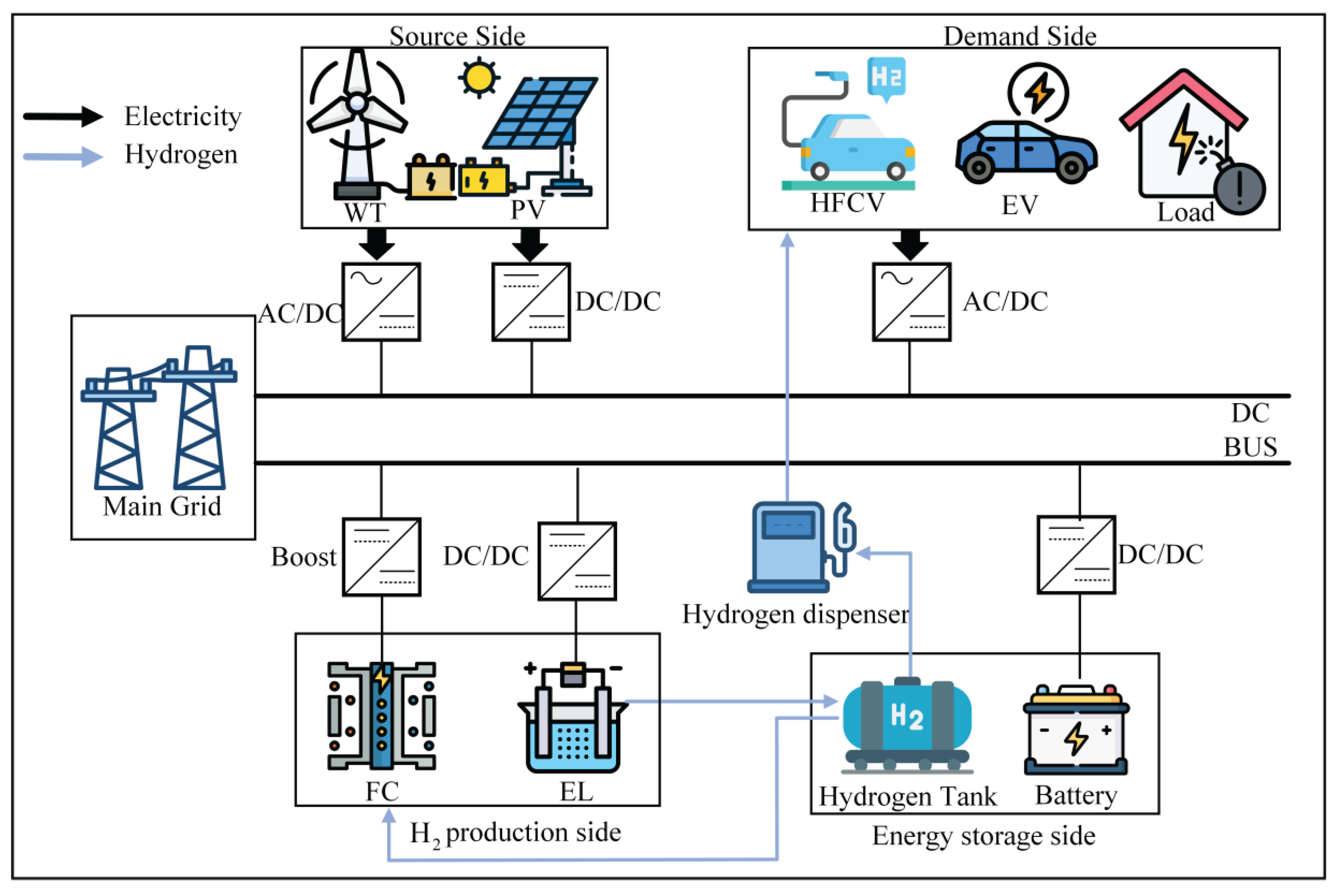
Figure 2.
Efficiency-Power Curves of PEMEL and PEMFC (a) Power-efficiency curve of the PEMEL (b) Power-efficiency curve of the PEMFC.
Figure 2.
Efficiency-Power Curves of PEMEL and PEMFC (a) Power-efficiency curve of the PEMEL (b) Power-efficiency curve of the PEMFC.
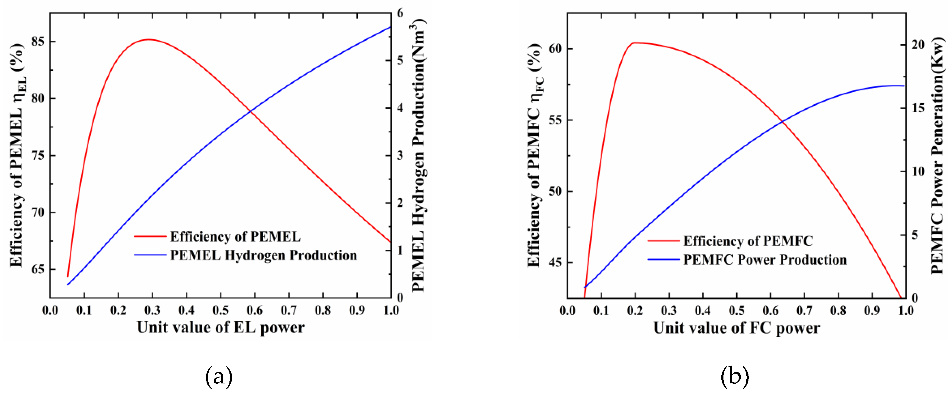
Figure 3.
Flowchart of LSTM-Based Source-Load Side Prediction.
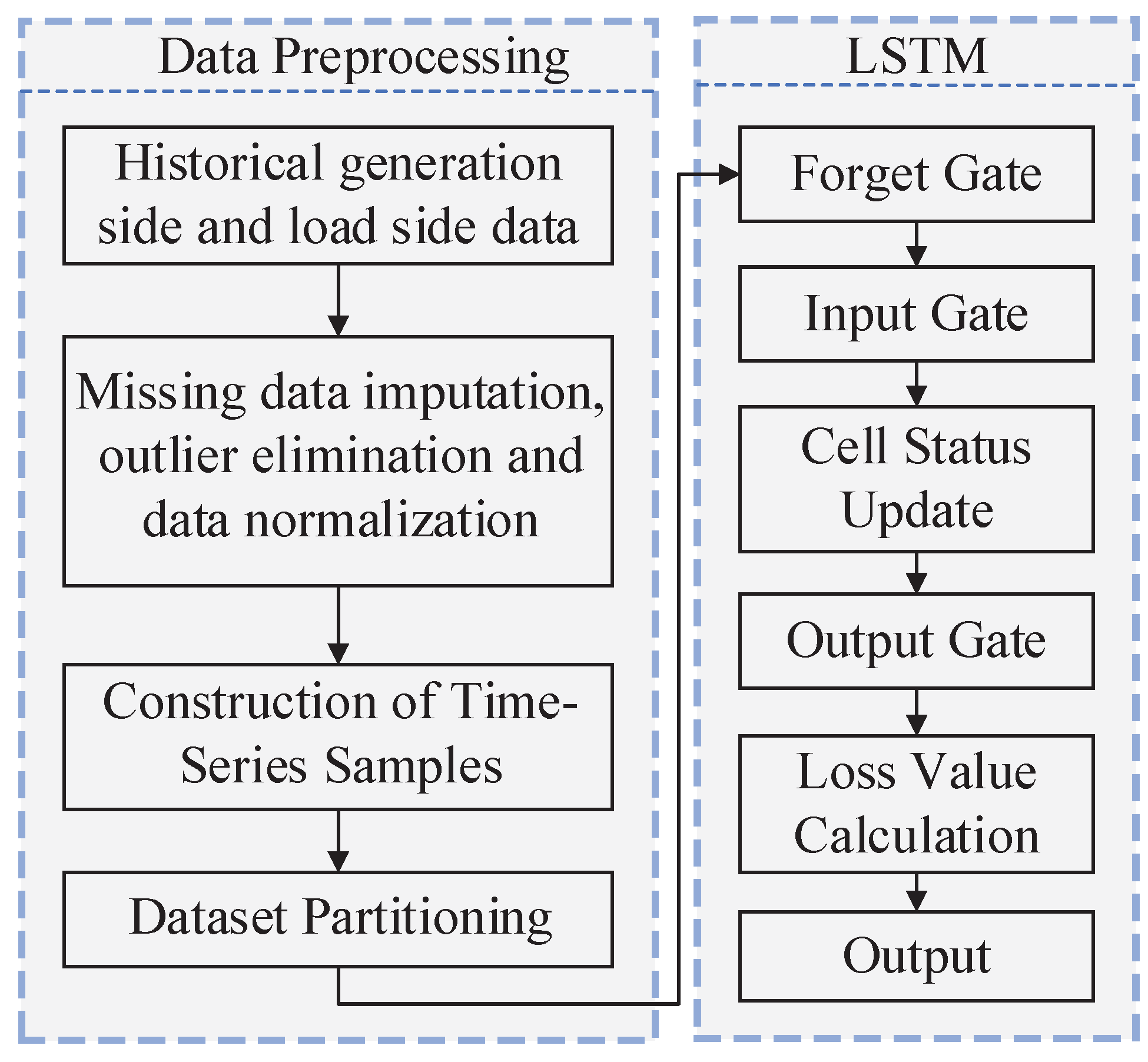
Figure 4.
Flowchart of the Algorithm.
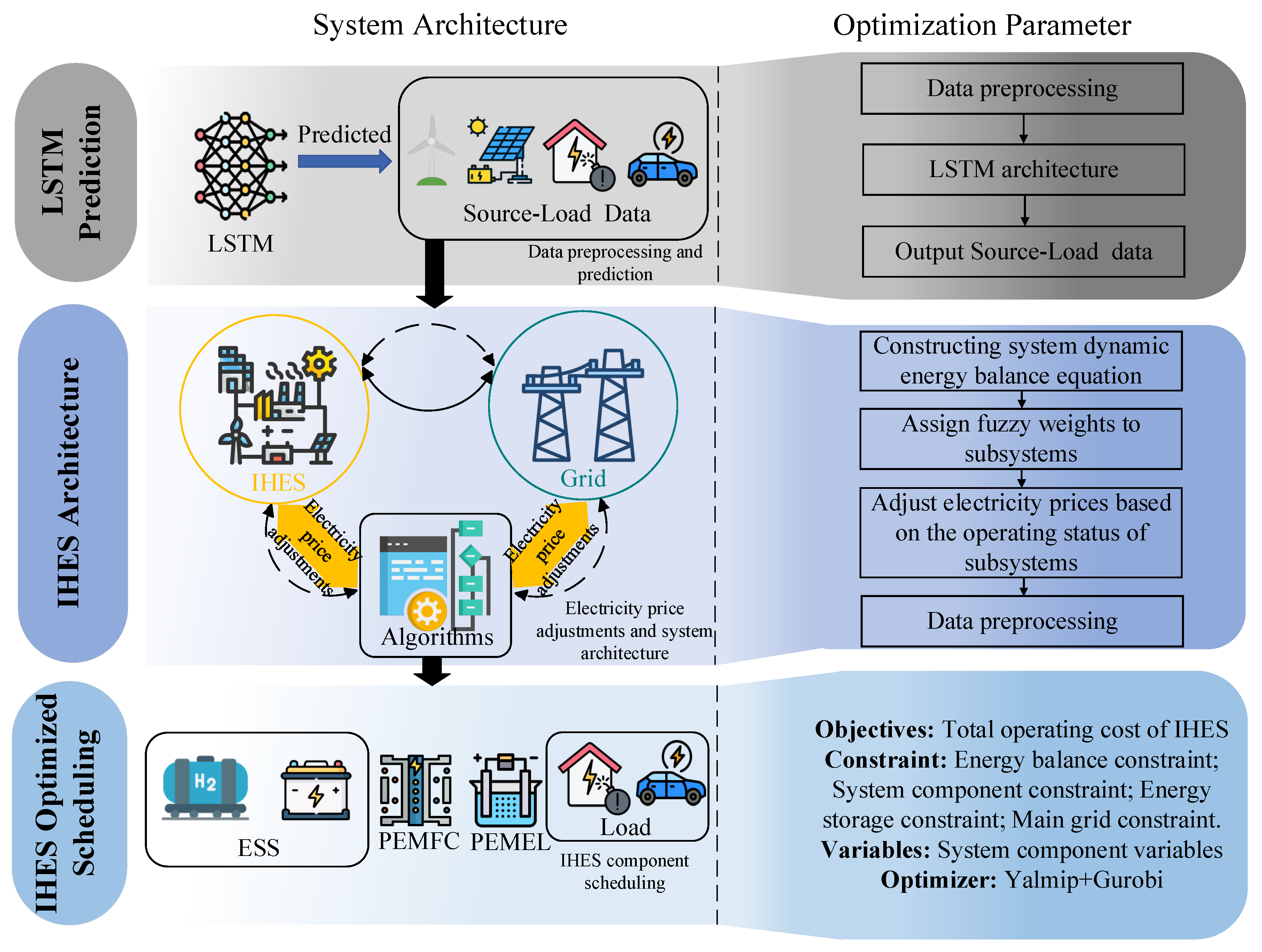
Figure 5.
Monthly predicted data of photovoltaic power generation, wind power generation, and load (a) Photovoltaic predicted data (b) Wind predicted data (c) Load predicted data.
Figure 5.
Monthly predicted data of photovoltaic power generation, wind power generation, and load (a) Photovoltaic predicted data (b) Wind predicted data (c) Load predicted data.
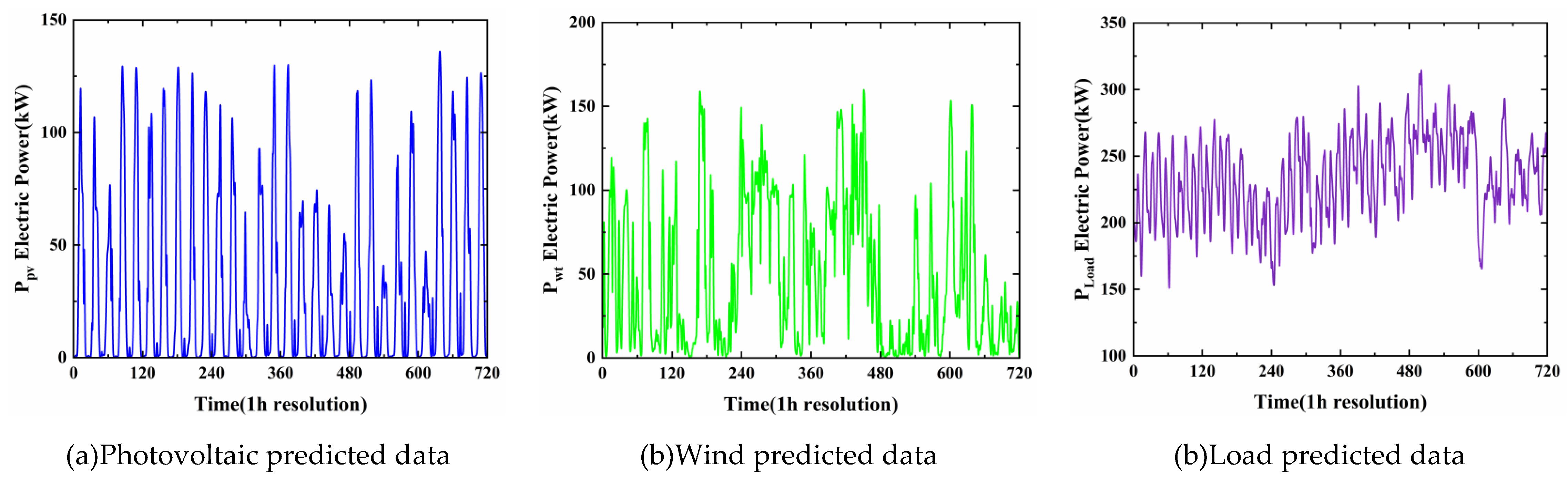
Figure 6.
Monthly predicted data error comparison of photovoltaic power generation, wind power generation and load (a) Photovoltaic error comparison (b) Wind error comparison (c) Load error comparison.
Figure 6.
Monthly predicted data error comparison of photovoltaic power generation, wind power generation and load (a) Photovoltaic error comparison (b) Wind error comparison (c) Load error comparison.
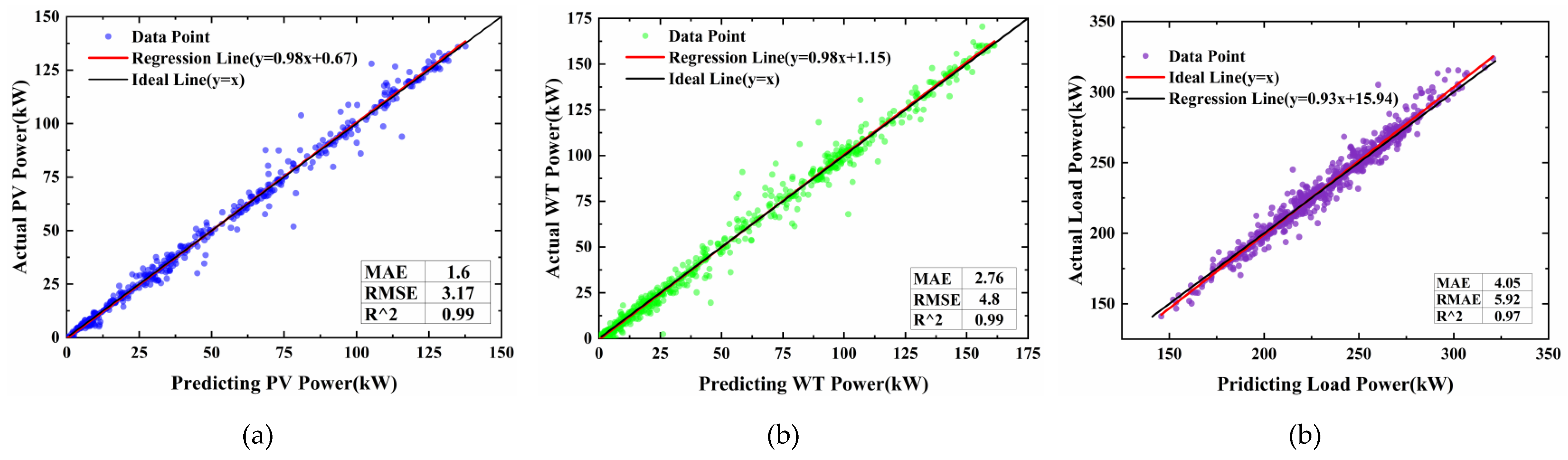
Figure 7.
PDF of Vehicle Owners’ Probabilistic Behaviors (a) PDF of arrival time for EVs and HFCVs (b) PDF of daily mileage for EVs and HFCVs.
Figure 7.
PDF of Vehicle Owners’ Probabilistic Behaviors (a) PDF of arrival time for EVs and HFCVs (b) PDF of daily mileage for EVs and HFCVs.
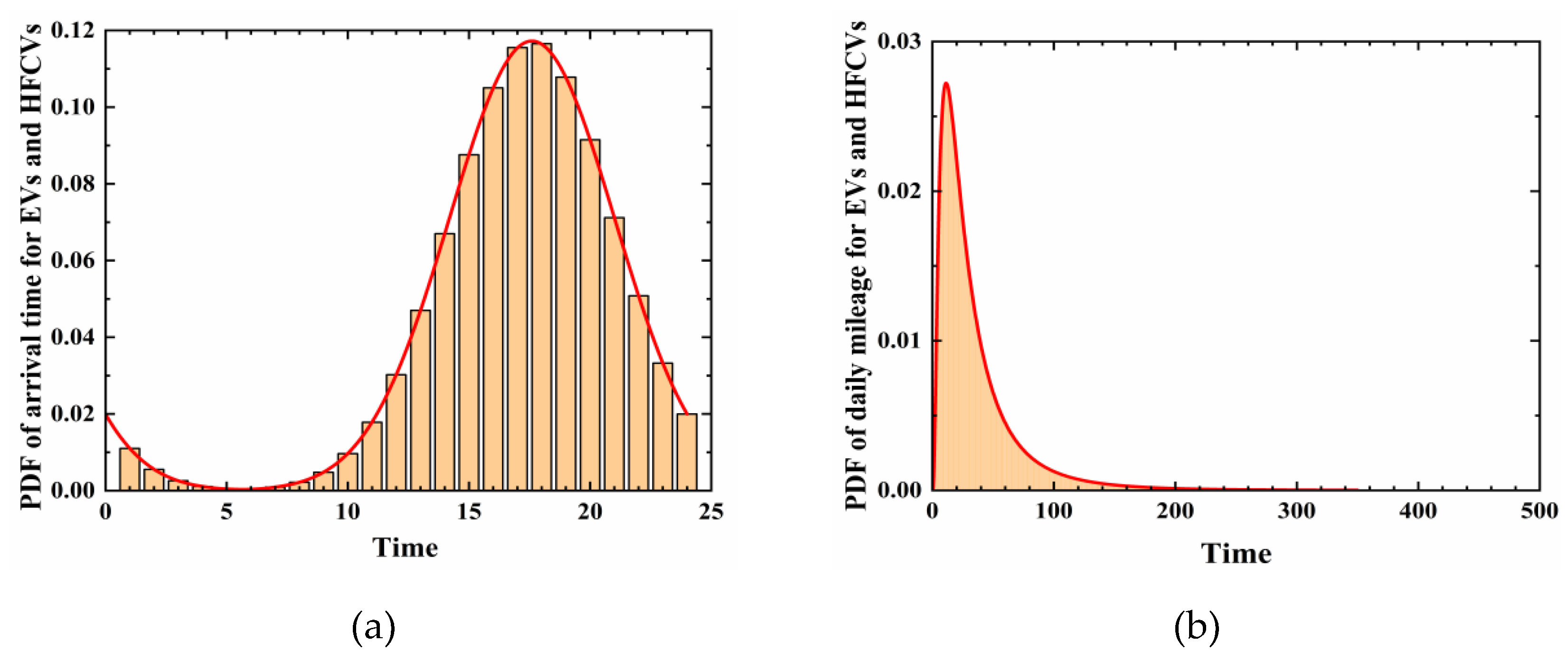
Figure 8.
Monte Carlo Simulation of Charging Load for Vehicles (a) EVs load demand curve (b) HFCVs load demand curve.
Figure 8.
Monte Carlo Simulation of Charging Load for Vehicles (a) EVs load demand curve (b) HFCVs load demand curve.
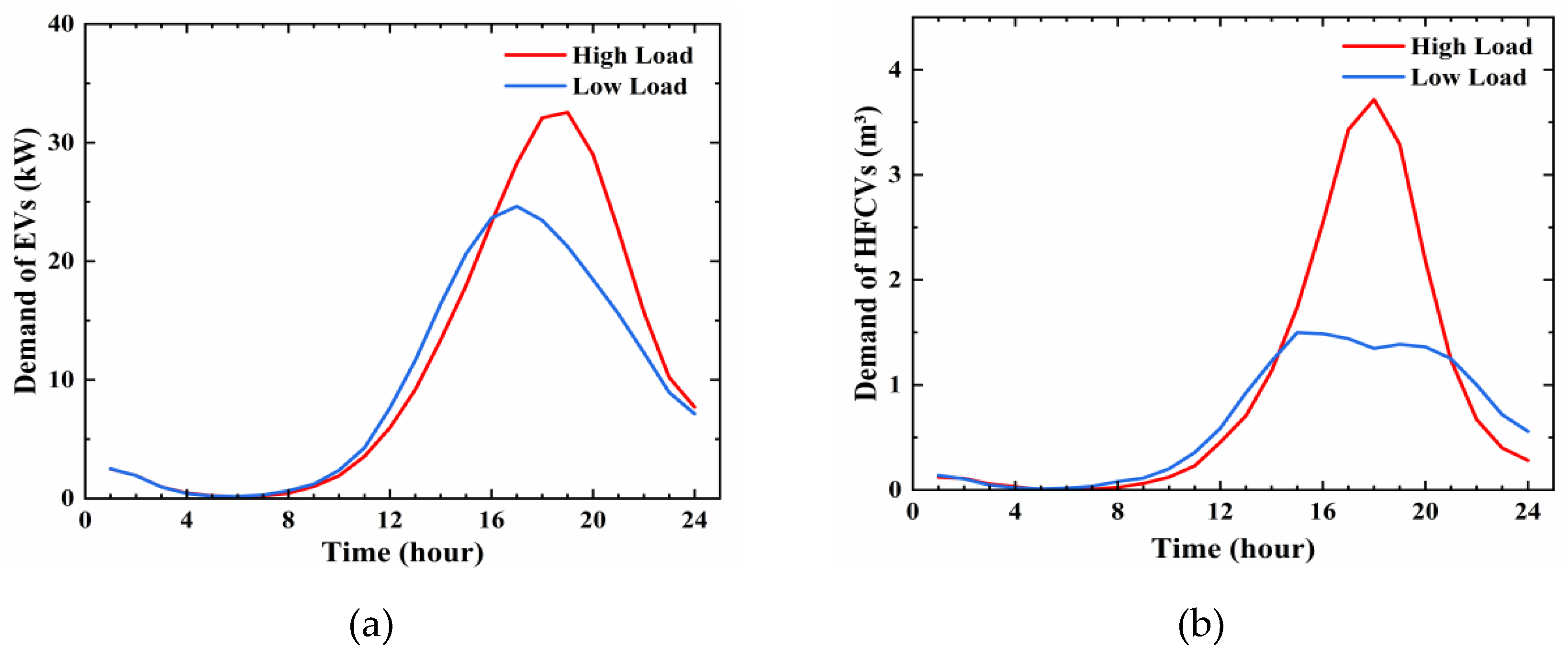
Figure 9.
Comparison of New Energy Power Generation and Load Forecasting (a) Typical day with high WT and PV power generation and high load (b) Typical day with low WT and PV power generation and low load.
Figure 9.
Comparison of New Energy Power Generation and Load Forecasting (a) Typical day with high WT and PV power generation and high load (b) Typical day with low WT and PV power generation and low load.
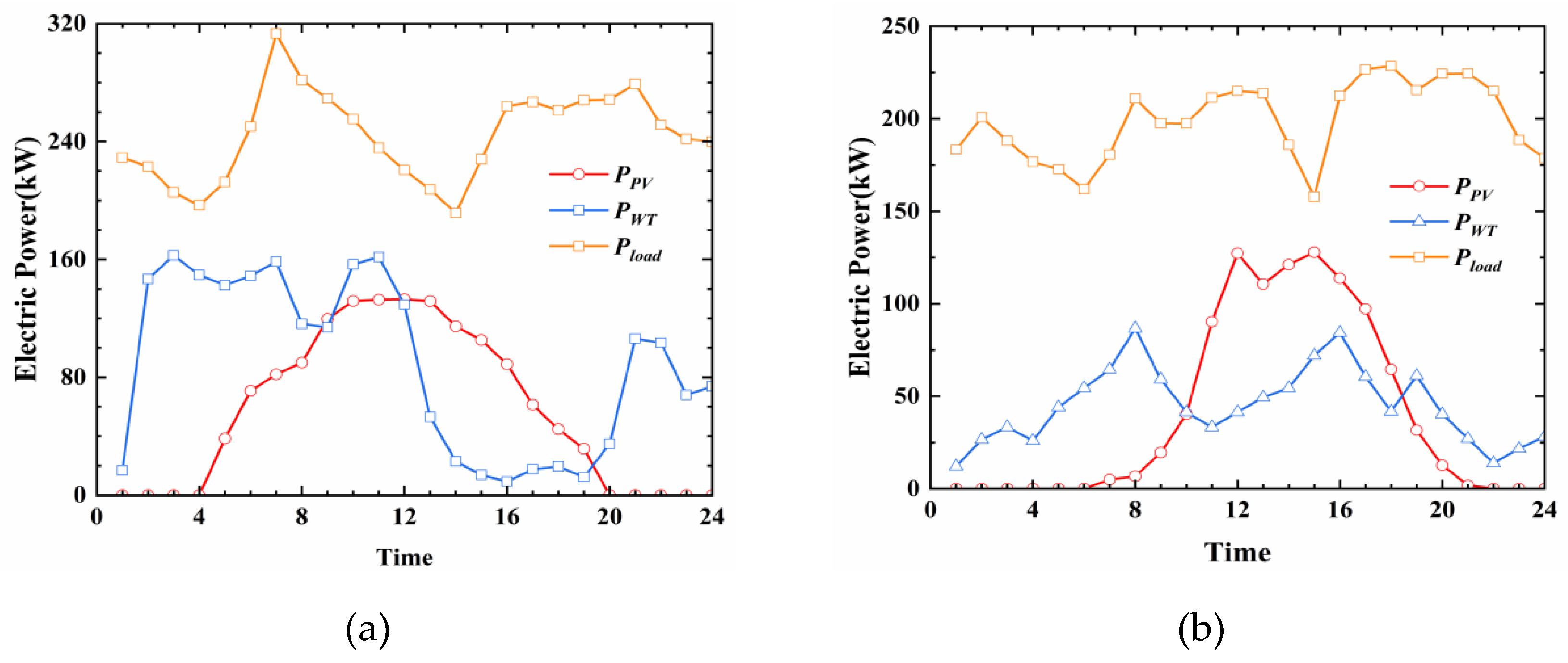
Figure 10.
Electricity Price on Dispatched Units and Load Reduction (a) Case I dynamic pricing strategy scheduling situation (b) Case I constant price strategy scheduling situation (c) Case II dynamic pricing strategy scheduling situation (d) Case II constant price strategy scheduling situation (e) Case III dynamic pricing strategy scheduling situation (f) Case III constant price strategy scheduling situation.
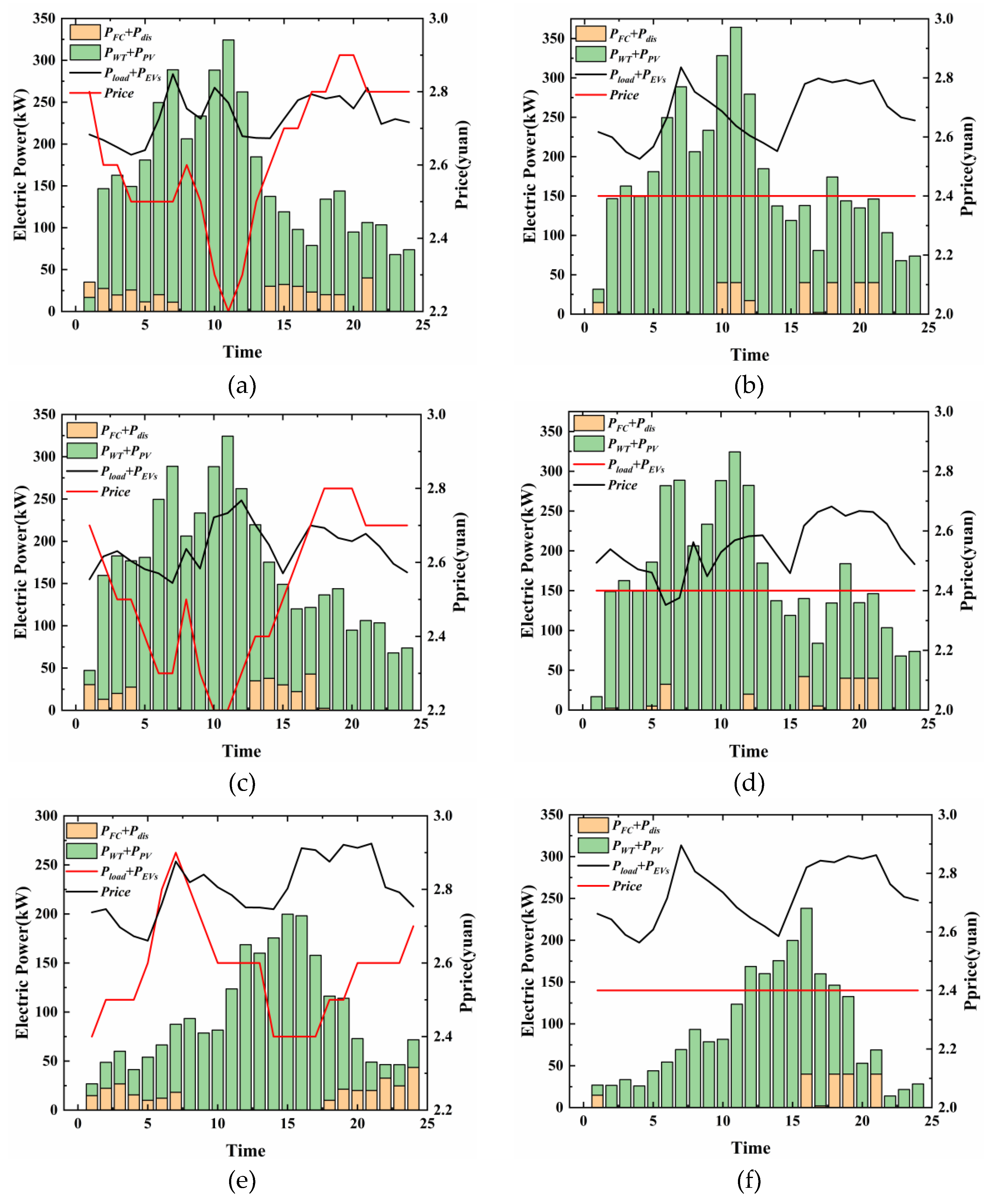
Figure 11.
Scheduling and Operation Results of Hydrogen Components (a) Case I dynamic pricing strategy hydrogen components scheduling situation (b) Case I constant price strategy hydrogen components scheduling situation (c) Case II hydrogen components scheduling situation (d) Case II hydrogen components scheduling situation (e) Case III hydrogen components scheduling situation (f) Case III hydrogen components scheduling situation scheduling situation.
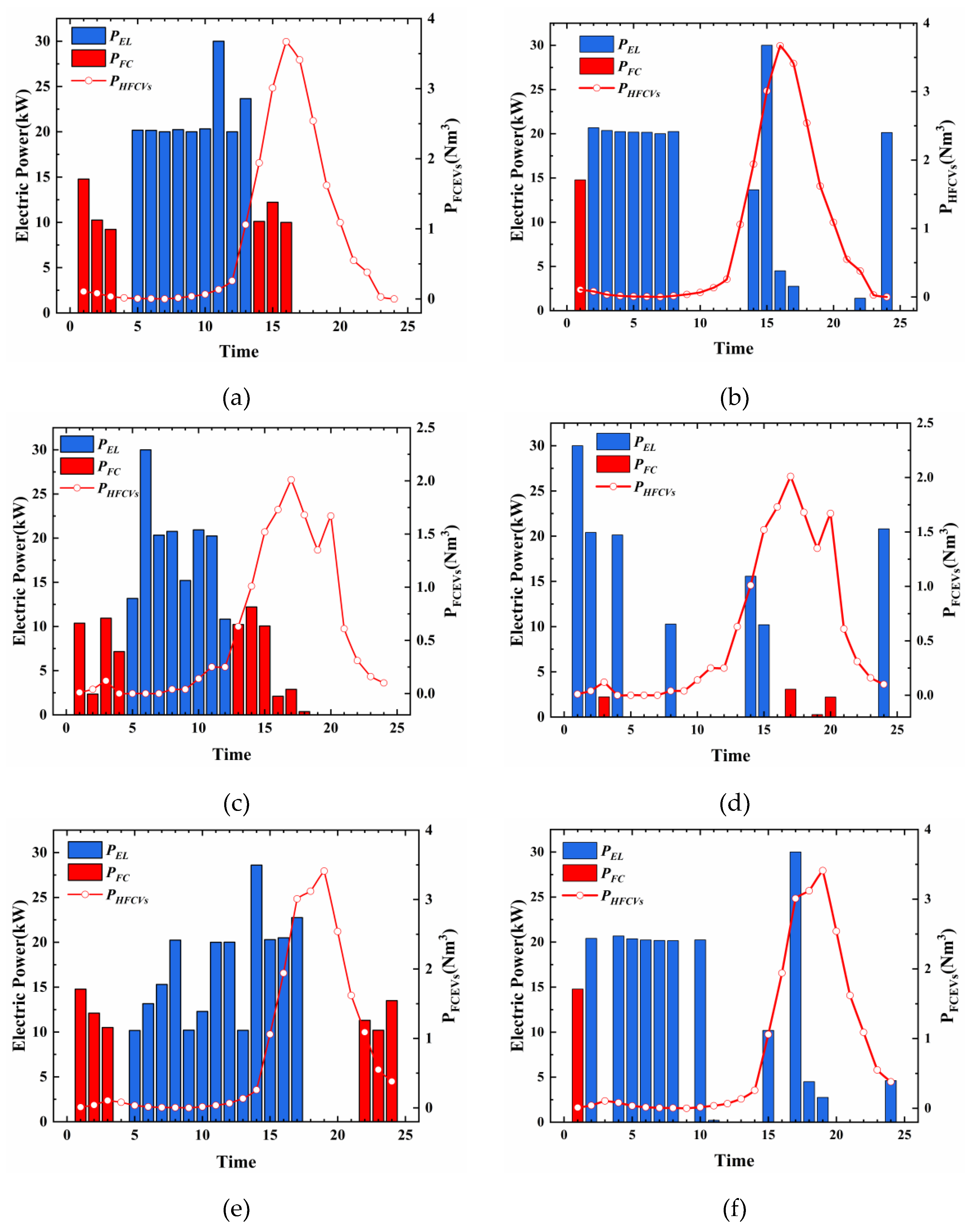
Figure 12.
Degradation of PEMEL and PEMFC (a) Dynamic pricing strategy degradation (b) Constant electricity price degradation.
Figure 12.
Degradation of PEMEL and PEMFC (a) Dynamic pricing strategy degradation (b) Constant electricity price degradation.
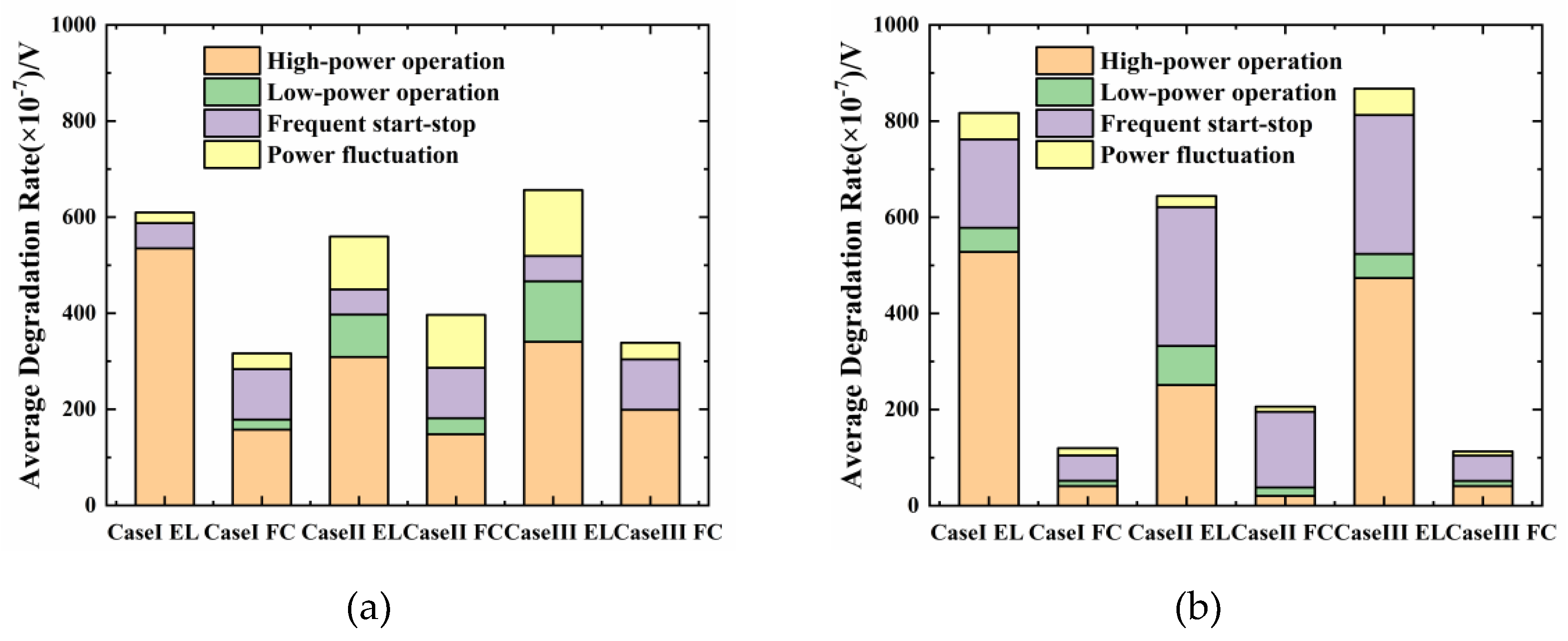
Figure 13.
Day-ahead scheduling results of three different scenarios (a) Case I dynamic pricing strategy system scheduling result (b) Case I constant price strategy system scheduling result (c) Case II dynamic pricing strategy system scheduling result (d) Case II constant price strategy system scheduling result (e) Case III dynamic pricing strategy system scheduling result (f) Case III constant price strategy system scheduling result.
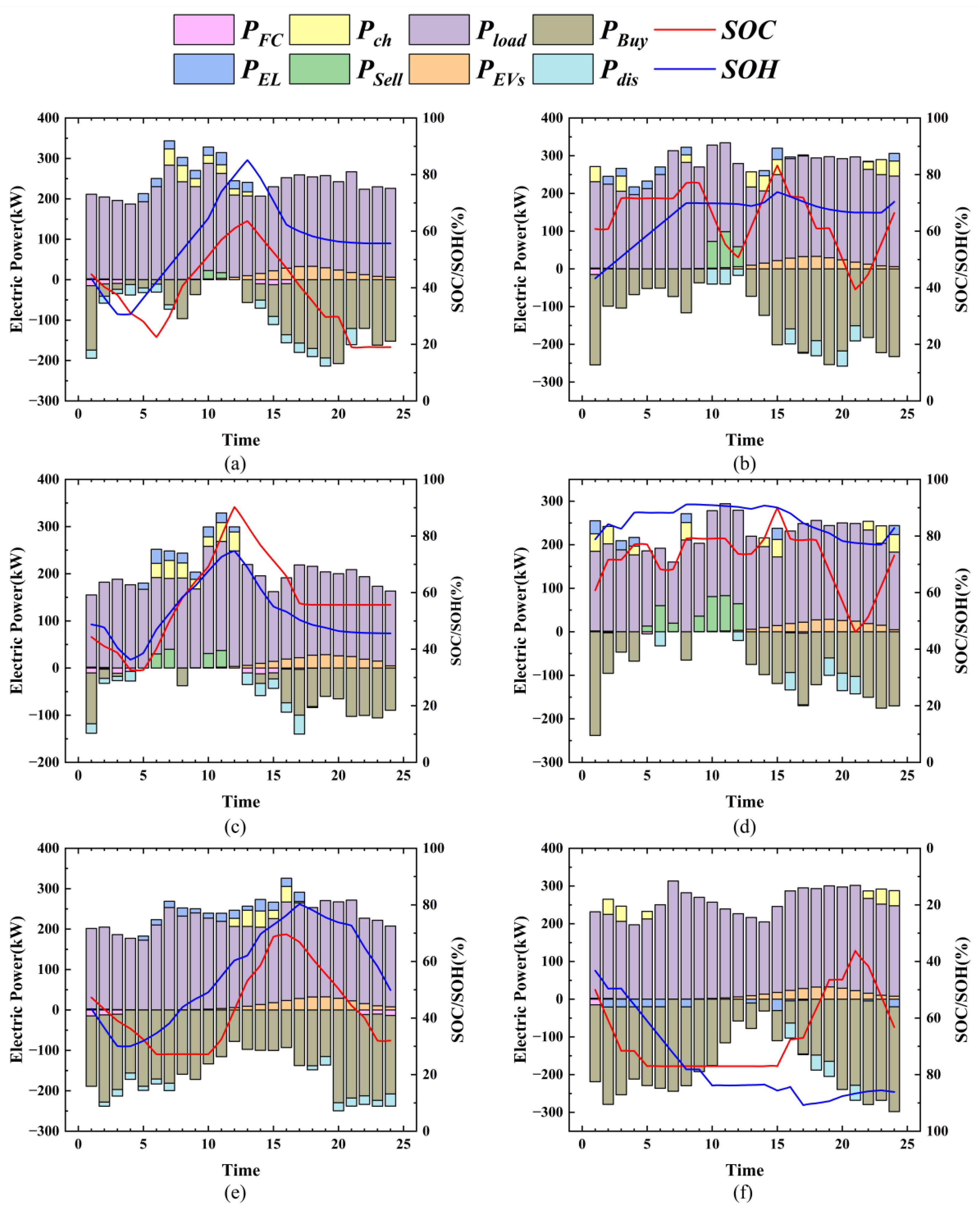
Figure 14.
Comparison of IHES operation costs (a) Case I comparison of operation costs (b) Case II comparison of operation costs (c) Case III comparison of operation costs.
Figure 14.
Comparison of IHES operation costs (a) Case I comparison of operation costs (b) Case II comparison of operation costs (c) Case III comparison of operation costs.
Disclaimer/Publisher’s Note: The statements, opinions and data contained in all publications are solely those of the individual author(s) and contributor(s) and not of MDPI and/or the editor(s). MDPI and/or the editor(s) disclaim responsibility for any injury to people or property resulting from any ideas, methods, instructions or products referred to in the content. |
© 2025 by the authors. Licensee MDPI, Basel, Switzerland. This article is an open access article distributed under the terms and conditions of the Creative Commons Attribution (CC BY) license (http://creativecommons.org/licenses/by/4.0/).
Copyright: This open access article is published under a Creative Commons CC BY 4.0 license, which permit the free download, distribution, and reuse, provided that the author and preprint are cited in any reuse.


