Submitted:
13 November 2024
Posted:
14 November 2024
You are already at the latest version
Abstract
In pursuit of dual-carbon objectives, establishing a low-carbon, efficient, and adaptable energy system has become a priority. This study introduces an advanced optimization scheduling model for integrated energy systems, enhancing system flexibility by optimizing combined heat and power (CHP) units, incorporating electric boilers and the Kalina cycle, and leveraging both electrical and thermal demand responses. A novel aspect of this model is the comprehensive integration of hydrogen production, utilization, and storage, forming an all-encompassing electricity-heat-gas-hydrogen framework. Simulation results validate the model's efficacy in minimizing operational costs and carbon emissions while improving renewable energy uptake.
Keywords:
Integrated Energy Systems
; Optimal Scheduling
; Hydrogen Energy Utilization
; Demand Response
; Low-Carbon Technologies
; Renewable Energy Integration
; System Flexibility
1. Introduction
As environmental concerns intensify, there is an
escalating urgency to innovate low-carbon, flexible, efficient, and
cost-effective energy solutions [1–3].
Integrated Energy Systems (IES) stand at the forefront of revolutionizing
traditional power infrastructures by seamlessly integrating various
heterogeneous energy sources and orchestrating the control across different
energy segments, which is crucial for achieving ambitious dual-carbon targets [4].
IES is distinguished by its substantial inclusion
of renewable energies, characterized by multi-energy coupling and low-carbon
cleanliness. This positions the low-carbon operation of IES as a focal point of
contemporary research [5–7]. One of the
integral components of IES, the Combined Heat and Power (CHP) unit, often
encounters operational challenges due to its static heat-to-power ratio, which
struggles to adapt to the dynamic demands of electrical and thermal loads [8–10]. To address this, several decoupling
strategies have been proposed. These include augmenting CHP units with thermal
storage or electric boilers to enhance peak-shifting flexibility [11], modifying steam flows and integrating make-up
combustion devices to achieve cogeneration decoupling [12], or employing an Organic Rankine Cycle (ORC) to
facilitate economic dispatch [13]. These
solutions aim to modulate the rigid heat-to-electricity ratios, yet
predominantly focus on single-mode decoupling, either “heat-to-electricity” or “electricity-to-heat”,
without addressing simultaneous dual-mode modifications. Additionally, despite
its superior efficiency in waste heat recovery, the Kalina cycle remains
underrepresented compared to ORC in scholarly studies [14,15].
Demand-side response (DSR) emerges as a crucial
regulatory resource within IES, capable of augmenting system flexibility and
diminishing the disparities between peak and valley load periods [16]. Innovations such as the integrated demand
response (IDR) model amalgamate the flexible characteristics of electricity,
heat, and gas loads with their interconnections, thus magnifying the regulatory
capacity of flexible loads [17].
Incentive-based IDR models have shown significant improvements in the energy
efficiency and economic performance of IES by tailoring responses for
electricity, industrial heat, and residential heating demands [18]. Additionally, hybrid IDR models that consider
varying time scales aim to stabilize the substantial power fluctuations within
the system [19]. However, these regulatory
capabilities are somewhat constrained by the potential impacts on user comfort
resulting from load adjustments. Optimal coordination between the source and
load sides could substantially enhance the responsiveness of these systems, a
topic that has not been extensively explored [20,21].
Hydrogen energy, recognized for its low-carbon and
clean properties, offers another viable strategy to meet dual-carbon objectives
by integrating into the traditional electric-thermal-gas IES frameworks [22]. Research has explored the multifaceted roles
of fuel cells and electrolyzers, investigating models that support the combined
supply and storage of heat, electricity, and hydrogen [23]. Other studies have proposed IES optimization
models that incorporate hydrogen storage within park ecosystems, undertaking
electrochemical and thermodynamic evaluations to devise optimal hydrogen
storage strategies [24]. Furthermore,
utilizing hydrogen as a conversion medium has prompted the development of
innovative low-carbon IES models that consider the flexible demands of
electrical and thermal loads alongside models for hydrogen utilization [25]. However, most existing research on
hydrogen-fueled IES has been limited to one or two utilization scenarios, often
overlooking the broader applications such as hydrogen production, usage, gas
blending, and storage—thus not fully leveraging the potential efficiencies of
hydrogen energy [26–28].
Addressing these gaps, this paper introduces a
pioneering IES model that incorporates dual-sided demand response and extensive
hydrogen utilization. Initially, the Kalina cycle and electric boilers are
integrated into the CHP units on the source side to decouple the conventional “heat
for electricity” and “electricity for heat” limitations, establishing a CHP
thermoelectric flexible response model. Concurrently, an electricity and heat
IDR model based on real-time pricing and thermal comfort is introduced on the
load side and synergized with the CHP flexible response model on the source
side to form a comprehensive dual-sided demand response framework.
Subsequently, a multi-utilization hydrogen model that includes hydrogen
production, utilization, gas mixing, and storage is embedded into the
electricity-heat-gas model, culminating in a novel
electricity-heat-gas-hydrogen IES low-carbon optimal dispatch model. The
efficacy of this proposed model and methodology is corroborated through
multiple application scenarios, illustrating its potential to transform energy
system operations comprehensively.
2. Source-Load Bilateral Demand Response Modeling
The source-load dual-side demand response model
constructed in this paper integrates the source-side CHP flexible response
model and the load-side electric heat demand response model. The CHP
cogeneration flexible response model on the source side can flexibly adjust the
output of electricity and heat, thus achieving similar effects with the
electric heat IDR model on the load side. Therefore, combining the source-side
CHP flexible response model with the load-side IDR model can form a
comprehensive source-load dual-side demand response model that optimizes the
energy efficiency and responsiveness of the entire system.
2.1. CHP Thermoelectric Flexible Response Model
Conventional cogeneration models usually consist of
a Gas Turbine (GT) and a Waste Heat Boiler (WHB), which are often operated in
“heat for electricity” or “electricity for heat” mode [29–32]. Since the peak-to-valley difference between
electricity and heat loads is often opposite, this fixed heat-to-power ratio
output makes it difficult to match CHP with demand fluctuations, thus limiting
the operational flexibility of integrated energy systems. In order to solve
this problem, this paper introduces the Kalina cycle and electric boiler model
into the CHP unit, which can decouple its “heat-to-electricity” or
“heat-to-electricity” modes, forming a CHP thermoelectric model that can
flexibly respond to the demand fluctuations. The GT model can be expressed as follows
[33–35]:
where and are the electric and thermal power output from GT;
and are the electric and thermal power conversion
efficiencies of GT; is the gas power input to GT; and are the upper and lower limits of the gas power
input to GT; and
are
the upper and lower limits of the creep rate of the gas power input to GT,
respectively.
With the introduction of the EB model and Kalina
cycle, the electrical energy output from the gas turbine (can flow to the EB
and electrical loads, respectively, while the thermal energy output from the GT
can flow to the waste heat boiler and Kalina cycle, respectively, which can be
expressed as follows [36]:
where is
the electric power fed into the electrical subsystem by the GT; is
the electric power fed into the EB by the GT; is
the thermal power fed into the Kalina cycle by the GT; , , and
are the upper limit values of, and , respectively.
Therefore, the electrical and thermal flexible
output model of CHP can be expressed as:
where and are the total electric and thermal power output
from the modified CHP; and are the electric power output from the Kalina
cycle and its thermal transfer efficiency; and are
the thermal power output from the EB and its thermal transfer efficiency; and are
the thermal power output from the WHB and its thermal transfer efficiency,
respectively.
2.2. Electricity and Heat Demand Response Modeling
2.2.1. Electric Load Response Modeling
In this paper, an elastic matrix response model
based on real-time tariff optimization is used to characterize the IDR model of
electric load. The real-time tariff can more accurately reflect the change of
supply and demand relationship in IES and dynamically guide the users to adjust
the energy load compared with the traditional time-of-day tariff [37–39], and its model can be expressed as follows:
where T denotes the dispatching period; is the elasticity matrix of real-time tariff; is the amount of electric load change after IDR; is the initial electric load; is the tariff base value; is the initial tariff; is the real-time base tariff fluctuation coefficient [40].
The amount of electric load transfer and the amount of tariff change are subject to the following constraints:
where is the upper limit of electric load variation; and are the minimum and maximum values of real-time tariffs; and are the minimum and maximum values of real-time tariff fluctuation constraints, respectively.
With the introduction of tariff IDRs, customer satisfaction with energy use needs to be taken into account:
where is the lower limit of satisfaction of the customer’s electrical load.
2.2.2. Thermal Load Response Modeling
Temperature, as the main indicator for regulating the heat load, allows the heat load to be adjusted within a specified range according to changes in the indoor temperature under the premise of ensuring the comfort of users [41,42,43]. For example, when the heat load demand reaches the peak, the heat load can be reduced by lowering the indoor temperature, thus reducing the pressure on power generation under the “heat for power” mode of the CHP system. On the contrary, during the low demand, increasing the indoor temperature can accumulate heat and utilize the energy during off-peak hours to increase the energy efficiency of the system [44]. Based on the thermal circuit model of a building, the relationship between user heat load and temperature can be expressed as [45,46]:
where R is the equivalent thermal resistance of the building; Cair is the indoor air heat capacity of the building; is the thermal power of the building; and denote the indoor and outdoor temperatures of the building, respectively.
3. Modeling of Multiple Uses of Hydrogen Energy
3.1. Electric Hydrogen Generation Segment
Electrolytic (EL) tank is the main equipment for electric hydrogen production, EL can convert the surplus electric energy into hydrogen energy, and considering the waste heat utilization of the electrolysis process [49,50], its energy conversion model can be expressed as follows:
where is the electric-hydrogen conversion efficiency of the EL; is the amount of hydrogen corresponding to 1kWh of electricity; is the input electric power of the EL; and are the maximum and minimum values of the; is the amount of hydrogen produced by the EL; is the amount of residual heat recovered by the EL; and are the maximum and minimum values of the creep rate.
3.2. Hydrogen to Cogeneration Link
Hydrogen Fuel Cell (HFC) can realize the coupling between hydrogen energy and thermal and electrical energy to realize the efficient use of hydrogen energy, and its model can be expressed as [51,52,53]:
where and are the electric and thermal conversion efficiency of HFC, respectively; is the input hydrogen power of HFC; and are the electric and thermal power of HFC, respectively; and are the maximum and minimum values of and are the maximum and minimum values of the ’s creep rate, respectively.
3.3. Hydrogen Methanation Link
The methane reactor (MR) converts the hydrogen produced by the EL to gas energy, and its energy conversion is modeled as [54,55,56]:
where and are the hydrogen consumption power of MR and the gas production power of MR, respectively; is the reaction efficiency of methanation; and are the maximum and minimum values of ; and are the maximum and minimum values of the ’s creep rate, respectively.
3.4. Natural Gas Hydrogen Blending Link
Mixing a certain proportion of hydrogen in the natural gas pipeline can increase the utilization path of hydrogen as well as improve the energy utilization efficiency [18]. Assuming that hydrogen is uniformly distributed in the natural gas pipeline, the proportion of hydrogen mixed with gas at time period t can be expressed as [57]
where is the proportion of hydrogen mixed with gas; is the total amount of hydrogen mixed with natural gas; is the amount of hydrogen fed into the GT; is the low calorific value of hydrogen; is the amount of natural gas fed into the GT; is the low calorific value of natural gas
Because more hydrogen doping will lead to “hydrogen embrittlement” phenomenon, so the proportion of hydrogen doping shall not exceed 20%, then there are [58,59,60]:
Therefore, the total amount of hydrogen mixed with natural gas after hydrogen blending can be expressed as:
where is the low calorific value of natural gas mixed with hydrogen gas.
3.5. Hydrogen Storage Link
In this paper, the high-pressure gaseous hydrogen storage technology is selected to model the hydrogen energy storage (HES) tank, i.e., [61]:
where and are the pressure inside the HES tank and its upper limit, respectively; is the amount of hydrogen stored in the HES; and are the density and relative molecular mass of hydrogen, respectively; is the molar gas constant; is the temperature of the gas inside the HES tank; and are the rate of hydrogen charging and discharging in the HES tank; and is the power of hydrogen charging and discharging, respectively. is the tank volume of the HES; is the hydrogen storage state of the HES. and are the maximum values of hydrogen charging power and hydrogen discharging power, respectively.
4. IES Scheduling Model
4.1. Objective Function
In this paper, the lowest total operating cost of IES is taken as the optimization objective for low-carbon economic dispatch, and its objective function can be expressed as follows:
where is the cost of carbon trading; and are the cost of purchasing electricity and gas; is the cost of equipment operation and maintenance; and is the cost of wind abandonment. The rest of the equation can be expressed as follows:
(1) Carbon trading costs C1
The baseline method is used to allocate carbon allowances to IES, which consists of three main components, namely, purchased electricity, GT and GB. In addition, a portion of carbon dioxide can be absorbed when converting hydrogen to natural gas in MR, so the carbon allowances of IES are allocated as follows:
where is the free carbon allowance of IES for purchasing electricity from the external grid; and are the free carbon allowances of CHP and GB, respectively; and are the carbon emission allocation coefficients per unit of electricity and per unit of heat, respectively; is the purchased power of the system; is the amount of carbon dioxide absorbed by the MR; is the electricity-heat conversion coefficient; is the total carbon allowance of the IES; is the efficiency of carbon dioxide absorption by the MR; is the purchased electricity of the IES; and is the heat output of the GB.
Therefore, the carbon trading cost borne by IES can be expressed as follows:
where is the price per unit of carbon traded; is the actual carbon emissions of IES, which can be calculated in the literature [62].
(2) Cost of electricity and gas purchases C2
where: and are the price of electricity and gas purchased by IES from the external grid, respectively; is the amount of natural gas imported by GB.
(3) Equipment operation and maintenance costs C3
where i and j are the types of energy conversion equipment and energy storage equipment, respectively; is the output power of energy conversion equipment i; and the charging and discharging power of energy storage equipment j, respectively; is the operation and maintenance coefficients of energy conversion equipment i; and is the operation and maintenance coefficients of energy storage equipment j.
(4) Wind abandonment costs C4
where is the cost per unit of wind penalty; is the power of wind power on-line; is the predicted power of wind power
4.2. Restrictive Condition
(1)Equipment operating constraints
The operating constraints for the GT, WHB, EB, Kalina cycles and the involved hydrogen multiple utilization models in IES can be found in Eqs. (1)-(3) and (11)-(18) and will not be repeated here. And the operational constraints of the battery (BT) and heat storage tank (HST) can be expressed as [63]:
where k ∈ {BT, HST}; and are the operating states of the energy storage device k, respectively; is the energy storage capacity of the energy storage device k; is the upper limit value ; and are the charging and discharging efficiencies of the kth type of energy storage device, respectively; is the upper limit value; and are the minimum and maximum values, respectively.
(2)Interacting power constraint
where is the upper purchased gas power of the IES; and are the upper purchased power limit and upper purchased gas power limit, respectively [64].
(3)Power balance constraints
where and are the charging and discharging power of BT, respectively; and are the charging and discharging thermal power of HST, respectively [65].
5. Case Study
5.1. System Settings
In order to verify the effectiveness of the proposed method, the IES topology diagram in Figure 1 is taken as an example to be analyzed. Among them, the electric and thermal load prediction curves and the wind power prediction curve are shown in Figure 2; the initial tariff is shown in Table 1; the IES equipment parameters are shown in Table 2; the outdoor temperature is shown in Figure 3; the upper and lower constraints on the tariffs are taken as [0.35, 1.4] yuan/kWh; and are 18℃ and 24℃, respectively; and are 0.728t/(MWh) and 0.102t/(GJ), respectively.
5.2. Validation of the Effectiveness of Source-Load Bilateral Demand Response
5.2.1. Source-Side CHP Thermoelectric Flexible Response Analysis
In order to verify the effectiveness of the source-side CHP thermoelectric flexible response model, the following four scenarios are set up for comparative analysis:
Scenario 1: taking into account the traditional CHP IES scheduling model; Square Scenario 2: introducing the EB model on the basis of Scenario 1; Scenario 3: introducing the Kalina cycle model on the basis of Scenario 1; Scenario 4: forming the CHP thermoelectric flexible response model on the basis of Scenario 1 by introducing the EB model and the Kalina cycle at the same time.
Table 3 shows the cost comparison results of the four scenarios. Firstly, the cost comparison results of each scenario are analyzed. From Table 3, it can be seen that the total cost of IES and carbon emission are the highest in Scenario 1, while Scenario 2 and Scenario 3 decouple the CHP’s “heat by electricity” and “heat by electricity” modes, respectively, with the introduction of the EB model and the Kalina cycle model, respectively. “With the introduction of the EB model and the Kalina cycle model respectively, the total cost of CHP decreases by 4.16% and 4.57%, and the total carbon emission decreases by 3.82% and 7.32% compared with Scenario 1, respectively. For Scenario 4, due to the introduction of both EB and Kalina cycles to realize the flexible output of CHP thermoelectricity, the total cost of its IES decreases by 4.32% and 3.91% compared with Scenario 2 and Scenario 3, respectively, and the total amount of carbon emission decreases by 7.19% and 3.68% compared with Scenario 2 and Scenario 3, respectively, which verifies the validity of the CHP thermoelectricity flexible response model proposed in this paper.
As can be seen in Figure 4 and Figure 5, wind power consumption is lowest in Scenario 1, which is mainly due to the peak-to-valley difference between electricity and heat loads and the operational constraints of the CHP system. The fixed patterns of “heat for electricity” and “electricity for heat” limit their flexibility during the peak hours of 22:00-24:00 and 01:00-06:00 at night, and the waste heat boiler needs to generate a large amount of heat to meet the heat demand, which leads to an increase in the power output of the gas turbine, thus failing to effectively utilize the available wind power. power output to increase, thus failing to effectively utilize the available wind resource. This situation makes IES show the lowest operational flexibility in Scenario 1.
In Scenario 2, the application of an electric boiler allows for the complete conversion of gas turbine power to heating energy from 11 p.m. to 7 a.m., thus breaking the conventional constraint of “heat for electricity”. This shift significantly enhances the utilization of wind power at night, although the constraint of “heat for electricity” remains. Moving on to Scenario 3, the addition of the Kalina cycle allows the GT to convert a portion of its thermal output into electricity, removing the “heat to power” constraint, which helps to alleviate the pressure during peak hours and reduces the need to purchase external power [66]. As for Scenario 4, the CHP system achieves complete decoupling between the dual constraints of “heat for electricity” and “heat for electricity” by integrating both EB and Kalina cycle technologies. As shown in Figure 5, this measure makes the CHP’s thermoelectric output extremely flexible and enhances the adjustment and response capability of the whole system.
Figure 6s and 7 show the distribution of electrical and thermal power from the gas turbine (GT) in scenario 4, as well as the results of the electrical and thermal energy balance. From these figures, it can be seen that during the nighttime hours of 23:00-24:00 and 01:00-07:00, due to the high wind power, the electrical power generated by the GT is used exclusively to drive the electric boiler to generate thermal energy, thus increasing the consumption of wind power. During the daytime hours of 10:00-20:00, part of the thermal output of the GT is used to drive the Kalina cycle to generate electricity, thus reducing the demand for electricity purchased from the external grid by the IES, due to the similarly high level of electric loads and electricity prices. In addition, according to the data in Table 3, Scenario 4 is the lowest in terms of total IES cost and carbon emissions, which verifies the high efficiency of the CHP thermoelectric flexible demand response model. Meanwhile, the peak-to-valley regulation of electric and thermal loads is also effectively supported by energy storage devices-battery storage and thermal storage-which charge energy during load troughs and release energy during peaks, further optimizing the load profile and demonstrating the important role of peak shaving and valley filling.
5.2.2. Load-side electrical and thermal IDR modeling analysis
In order to verify the validity of the proposed electric and thermal IDR models, the electric and thermal IDR models are introduced to form Scenario 5 based on Scenario 1. Table 4 shows the cost comparison results for Scenario 1 and Scenario 5. Figure 8 shows the load, wind and GT comparison results for Scenario 1 and Scenario 5.
From the data analysis in Table 4 and Figure 8, it can be seen that the high output characteristics of wind power in the evening lead to a high abandonment rate. In Scenario 5, by adjusting these peak electric load hours of 10:00-12:00 and 15:00-19:00 to the high wind power output hours of 23:00-07:00, the nighttime wind power dissipation capacity is effectively improved. In addition, as shown in Figure 8b,d, by responding to the thermal load adjustment, the nighttime peak thermal load is reduced, which correspondingly reduces the electrical output of gas turbines (GTs) and provides more accommodating space for wind power to be connected to the grid. From Figure 8(c), it is observed that in Scenario 5, the efficiency of wind power consumption is significantly better than that of Scenario 1. According to Table 4, compared with Scenario 1, the integrated energy system (IES) of Scenario 5 reduces the total cost, wind abandonment loss, and carbon emission by 8.79%, 40.9%, and 10.93%, respectively, which are the results proving that the electric and thermal demand response models have a Significant effect.
5.2.3. Flexible Demand Response Analysis for Source and Load Bilateral
In order to verify the effectiveness of source-load bilateral flexible demand response, Scenario 6 is added to compare and analyze with Scenario 4 and Scenario 5. Scenario 6 is the IES optimized operation model considering flexible demand response at source-load bilaterally. Table 5 shows the cost comparison results of the three scenarios. Figure 9 shows the power dispatch results of scenario 6 and the wind power consumption comparison results of the three scenarios, respectively.
According to the analysis in Figure 9, Scenario 6 integrates the source-side CHP thermoelectric flexible demand response model and the load-side electric and thermal IDR models, which enables the IES to flexibly adjust the thermoelectric output of the CHP according to the actual changes in electric and thermal loads. Compared with Scenarios 4 and 5, Scenario 6, by integrating the source-side and load-side strategies, not only realizes the transfer of peak electric loads to the valley hours, but also converts the excess nighttime electric energy into thermal energy through the electric boiler, which significantly improves the wind power consumption capacity and reduces the cost of energy purchases and carbon emissions. This result emphasizes that the economy and flexibility of the system can be significantly improved through the synergistic optimization of the source side and the load side.
5.3. Analysis of the effectiveness of multiple utilization of hydrogen energy
Next, the impact of the proposed hydrogen energy multiple utilization model on the optimal scheduling of the system is verified. In this paper, on the basis of Scenario 6, Scenario 7 and Scenario 8 are added for comparative analysis. Scenario 7: On the basis of scenario 6, a hydrogen energy utilization model composed of EL, MR, and HFC is introduced. Scenario 8: On the basis of Scenario 7, the gas hydrogen mixing link is introduced.
Table 5 shows the cost comparison results of Scenario 6-Scenario 8. Calculated from Table 5, it can be seen that compared with Scenario 6, the total cost and carbon emission of IES in Scenario 7 are decreased by 4.83% and 10.52%, respectively, and after the introduction of the hydrogen utilization model, the wind power of IES is completely consumed, which verifies the role of the hydrogen utilization model in this paper.
6. Conclusion
This study has developed a comprehensive low-carbon optimal dispatch model for integrated energy systems that incorporates both source and load-side demand responses along with extensive hydrogen energy utilization. This model strives to enhance the low-carbon and cost-effective operations through a synergistic source-load coordinated approach. From the analysis of practical examples, we derive several key insights:
(1) The proposed flexible response model for Combined Heat and Power integrates an electric boiler and the Kalina cycle, effectively decoupling the fixed “heat-determined electricity” and “electricity-determined heat” operational modes of CHP. This adaptation facilitates flexible thermoelectric output from the source side, markedly enhancing the system’s capacity to integrate renewable energy.
(2) By synchronizing the flexible demand response mechanisms from both the source and load sides, the model allows for adaptable adjustments in CHP output power. This alignment optimizes the electric and thermal load profiles concurrently, achieving an integrated optimization of both source and load. The results indicate that this model not only boosts the overall system flexibility but also significantly lowers both wind curtailment and operational costs.
(3) Incorporating a multi-faceted hydrogen utilization model, which includes electrolyzers, methane reactors, hydrogen Fuel Cells, and gas-hydrogen blending capabilities, the system can effectively harness and maximize the use of excess nighttime wind energy. This integration enhances the energy efficiency, cuts total carbon emissions, and reduces the operating expenses of the IES.
While this model demonstrates significant potential, it acknowledges certain limitations, such as the assumption of constant market conditions and regulatory environments, which may not hold in dynamic real-world settings. Future research should explore the adaptability of the model under fluctuating economic conditions and varying regulatory frameworks. Additionally, integrating artificial intelligence, as explored in the context of enhancing transient stability in power systems [67,68], could further optimize energy management and security in integrated energy systems. These directions promise to refine the scalability and applicability of the model, paving the way for more resilient and adaptable energy system frameworks.
References
- Zhang, S., Wang D., Cheng H., et al. Key Technologies and Challenges in Low-Carbon Integrated Energy System Planning under Dual Carbon Goals[J]. Automation of Electric Power Systems, 2022, 46(8): 189-207.
- Wang M, Wang M, Wang R, et al. Optimization scheduling for low-carbon operation of building integrated energy systems considering source-load uncertainty and user comfort[J]. Energy and Buildings, 2024, 318: 114423. [CrossRef]
- Kong W, Sun K, Zhao J. Two-Stage Optimal Scheduling of Community Integrated Energy System Considering Operation Sequences of Hydrogen Energy Storage Systems[J]. Journal of Modern Power Systems and Clean Energy, 2024.
- Jia S, Kang X, Cui J, et al. Hierarchical stochastic optimal scheduling of electric thermal hydrogen integrated energy system considering electric vehicles[J]. Energies, 2022, 15(15): 5509. [CrossRef]
- CHEN Changming, WU Xueyan, LI Yan, et al. Distributionally robust day-ahead scheduling of park-level integrated energy system considering generalized energy storages[J]. Applied Energy, 2021, 302: 117493. [CrossRef]
- Wei, Z., Huang Y., Gao H., et al. Combined Economic Dispatch of Regional Energy Internet with Power-to-Gas and Cogeneration Units Featuring Thermal and Electrolytic Decoupling [J]. Power System Technology, 2018, 42(11): 3512-3520.
- Wang Z, Du B, Li Y, et al. Multi-time scale scheduling optimization of integrated energy systems considering seasonal hydrogen utilization and multiple demand responses[J]. International Journal of Hydrogen Energy, 2024, 67: 728-749. [CrossRef]
- Liu, Z., Xing H., Cheng H., et al. Bi-level Optimization Scheduling of Integrated Energy Systems Considering Carbon Emissions Trading and Demand Response [J]. High Voltage Engineering, 2023, 49(1): 169-178.
- Wang X, Zhao Y, Sun W, et al. Optimal scheduling of integrated energy system for hydrogen production with electricity[J]. Engineering Reports, 2024: e12985.
- Wang, Y., Xie H., Sun X., et al. Day-ahead Economic Dispatch of Electric-thermal Integrated Energy Systems Considering Incentive-based Comprehensive Demand Response [J]. Transactions of China Electrotechnical Society, 2021, 36(09): 1926-1934.
- CHEN X, WU G, LONG Z, et al. Multi-time scale optimal dispatch of integrated energy systems considering source-load uncertainty and user-side demand response[J]. Journal of Electric Power Science and Technology, 2024, 39(3): 217-227.
- Chang P, Li C, Zhu Q, et al. Optimal scheduling of electricity and hydrogen integrated energy system considering multiple uncertainties[J]. Iscience, 2024, 27(5).
- Li, Q., Zou X., Pu Y., et al. Optimization Scheduling Method for Cogeneration Microgrid Based on Hydrogen Energy Storage [J]. Journal of Southwest Jiaotong University, 2023, 58(1): 9-21.
- Long X, Liu H, Wu T, et al. Optimal Scheduling of Source–Load Synergy in Rural Integrated Energy Systems Considering Complementary Biogas–Wind–Solar Utilization[J]. Energies, 2024, 17(13): 3066.
- Deng, J., Jiang F., Wang W., et al. Low-Carbon Operation of Integrated Energy Systems Considering Electric and Thermal Flexible Loads and Refined Hydrogen Energy Modeling [J]. Power System Technology, 2022, 46(05): 1692-1704.
- Gao, Y., Wang Q., Chen Y., et al. Optimization Scheduling of Hydrogen-containing Integrated Energy Systems Considering Demand Response and Energy Cascade Utilization [J]. Automation of Electric Power Systems, 2023, 47(04): 51-59.
- Xing Xuetao, Lin Jin, Song Yonghua, et al. Optimization of hydrogen yield of a high-temperature electrolysis system with coordinated temperature and feed factors at various loading conditions: a model-based study[J]. Applied Energy, 2018, 232: 368-385.
- MEHRJERDI H, SABOORI H, JADID S. Power-to-gas utilization in optimal sizing of hybrid power, water, and hydrogen microgrids with energy and gas storage[J]. Journal of Energy Storage, 2022, 45: 103745.
- Dong, S., Teng M., Pan Z., et al. Thermodynamic and Thermo-economic Analysis of a New Geothermal-driven Trigeneration System of Cold, Heat, and Power [J]. Acta Energiae Solaris Sinica, 2021, 42(05): 1-9.
- Zhou, W., Sun Y., Xie D., et al. Low-Carbon Scheduling of Campus Integrated Energy Systems Considering Improved Stepwise Carbon Trading and Flexible Output of Cogeneration Units [J/OL]. Power System Technology, 1-12 [2023-12-11].
- Li Y, Yang Z, Li G, et al. Optimal scheduling of an isolated microgrid with battery storage considering load and renewable generation uncertainties[J]. IEEE Transactions on Industrial Electronics, 2019, 66(2):1565-1575.
- Yu, Z., Ma J. Coordinated Dispatch Strategy of Multi-regional Integrated Energy Systems with Wind Power Coupled Hydrogen Production Using a Master-Slave Game Approach [J]. Electrical Technology, 2023, 24(7): 1-10.
- Zhang G, Wen J, Xie T, et al. Bi-layer economic scheduling for integrated energy system based on source-load coordinated carbon reduction[J]. Energy, 2023, 280: 128236.
- Liu, C., Liu W., Gao X., et al. Coordinated Planning of Distribution Network and Multi-integrated Energy Systems Based on Master-Slave Game [J]. Electric Power Automation Equipment, 2022, 42(6): 144-152.
- Wang Y, Dong P, Xu M, et al. Research on collaborative operation optimization of multi-energy stations in regional integrated energy system considering joint demand response[J]. International Journal of Electrical Power & Energy Systems, 2024, 155: 109507.
- Li Y, Bu F, Li Y, et al. Optimal scheduling of island integrated energy systems considering multi-uncertainties and hydrothermal simultaneous transmission: A deep reinforcement learning approach[J]. Applied Energy, 2023, 333:120540.
- Su S, Hu G, Li X, et al. Electricity-Carbon Interactive Optimal Dispatch ofMulti-Virtual Power Plant Considering Integrated Demand Response[J]. Energy Engineering, 2023, 120(10).
- Fang Z, Zhao D, Chen C, et al. Nonintrusive appliance identification with appliance-specific networks[J]. IEEE Transactions on Industry Applications, 2020, 56(4): 3443-3452.
- Wang C, Liu C, Zhou X, et al. Hierarchical Optimal Dispatch of Active Distribution Networks Considering Flexibility Auxiliary Service of Multi-community Integrated Energy Systems[J]. IEEE Transactions on Industry Applications, 2024.
- Wang, R., Cheng S., Wang Y., et al. Low-Carbon Economic Optimal Scheduling of Regional Integrated Energy Systems Based on Multi-agent Master-Slave Game [J]. Power System Protection and Control, 2022, 50(5): 12-21.
- Long X, Li Y, et al. Collaborative response of data center coupled with hydrogen storage system for renewable energy absorption[J]. IEEE Transactions on Sustainable Energy, 2024, 15(2): 986-1000.
- Xiong, Y., Si Y., Zheng T., et al. Optimization Allocation of Hydrogen Energy Storage in Industrial Park Integrated Energy Systems Based on Master-Slave Game [J]. Transactions of China Electrotechnical Society, 2021, 36(3): 507-516.
- Zhao, H., Miao S., Li C., et al. Study on the Optimal Operation Strategy of Campus Integrated Energy Systems Considering Coupled Response Characteristics of Cold, Heat, and Electricity Demands [J]. Proceedings of the CSEE, 2022, 42(2): 573-589.
- Wang, X., Chen H., Chen L. Multi-agent Interactive Decision Model for Enhancing Operational Flexibility of Regional Integrated Energy Systems [J]. Transactions of China Electrotechnical Society, 2021, 36(11): 2207-2219.
- Zhang G, Niu Y, Xie T, et al. Multi-level distributed demand response study for a multi-park integrated energy system[J]. Energy Reports, 2023, 9: 2676-2689.
- Wang, Y., Qi Y., Cai Y., et al. Coordinated Optimization Scheduling Strategy of “Source-Load-Storage” in Integrated Energy Systems Considering Equipment Variable Load Rate Characteristics [J]. Electric Measurement & Instrumentation, 2024, 61(7): 123-130.
- Li Y, Wang C, Li G, et al. Improving operational flexibility of integrated energy system with uncertain renewable generations considering thermal inertia of buildings[J]. Energy Conversion and Management, 2020, 207: 112526.
- Wang L, Cheng J, Luo X. Optimal scheduling model using the IGDT method for park integrated energy systems considering P2G–CCS and cloud energy storage[J]. Scientific Reports, 2024, 14(1): 17580.
- Wu, M., Shi J., Wang K., et al. Demand Response Strategy for Integrated Energy Systems with Electro-Hydrogen Storage in Carbon Market [J]. Modern Electric Power, 2023, 40(6): 947-956.
- Wang X, Li M, Chen S, et al. Optimization of Regional Integrated Energy System Cluster Based on Multi-agent Game[C]//2022 IEEE/IAS Industrial and Commercial Power System Asia (I&CPS Asia). IEEE, 2022: 533-538.
- Li Y, Han M, Shahidehpour M, et al. Data-driven distributionally robust scheduling of community integrated energy systems with uncertain renewable generations considering integrated demand response[J]. Applied Energy, 2023, 335: 120749.
- Jiang, T., Zhou H., Zhou W., et al. Optimization Scheduling of Regional Integrated Energy Systems Based on Source-Load Coordinated Peak Shaving [J]. Electrical Appliances and Energy Efficiency Management Technology, 2022 (9): 8.
- Chen, C., Wu C., Lin X., et al. Energy Buying and Selling Strategy for Integrated Energy Merchants in Parks Considering Upstream and Downstream Markets [J]. Transactions of China Electrotechnical Society, 2022, 37(1): 220-231.
- Chen L, Li Y, Huang M, et al. Robust dynamic state estimator of integrated energy systems based on natural gas partial differential equations[J]. IEEE Transactions on Industry Applications, 2022, 58(3): 3303-3312.
- Zhao, S., Han A., Zhou S., et al. Integrated Energy Optimization Scheduling Based on a Multi-objective Stackelberg Leader-Follower Game Model [J]. Journal of Electrical Engineering, 2023, 18(3): 341-347.
- Li Y, He S, Li Y, et al. Federated multiagent deep reinforcement learning approach via physics-informed reward for multimicrogrid energy management[J]. IEEE Transactions on Neural Networks and Learning Systems, 2024, 35(5):5902-5914.
- Zhao H, Yao Y, Peng D, et al. A preference adjustable capacity configuration optimization method for hydrogen-containing integrated energy system considering dynamic energy efficiency improvement and load fast tracking[J]. Renewable Energy, 2024: 121314.
- Li Y, Han M, Yang Z, et al. Coordinating flexible demand response and renewable uncertainties for scheduling of community integrated energy systems with an electric vehicle charging station: A bi-level approach[J]. IEEE Transactions on Sustainable Energy, 2021, 12(4):2321-2331.
- Sun, W., Wu J., Zhang Q. Optimization Scheduling Strategy Considering Electrical Energy Interaction Among Multi-regional Integrated Energy Systems Under Active Distribution Networks [J]. Science Technology and Engineering, 2024, 24(11): 539-548.
- Li, X., Li C., Zhang L. Bi-level Game Stochastic Optimization Scheduling Strategy for Hydrogen-Coupled Regional Integrated Energy System Clusters [J]. Electric Power Automation Equipment, 2023, 43(12): 201-210.
- Li Y, Wang B, Yang Z, et al. Optimal scheduling of integrated demand response-enabled community-integrated energy systems in uncertain environments[J]. IEEE Transactions on Industry Applications, 2021, 58(2): 2640-2651.
- Zhang Q, Qi J, Zhen L. Optimization of integrated energy system considering multi-energy collaboration in carbon-free hydrogen port[J]. Transportation Research Part E: Logistics and Transportation Review, 2023, 180: 103351.
- Wang, L., Lin J., Dong H., et al. Optimization Scheduling of Integrated Energy Systems Considering Stepwise Carbon Trading [J]. Journal of System Simulation, 2022, 34(7): 1393-1402.
- Cheng, Y., Guo Q. Bi-level Optimization Scheduling Strategy for Multi-agent Integrated Energy Systems Considering Dynamic Energy Prices and Shared Energy Storage Stations [J]. Modern Electric Power, 2024, 41(1): 10-20.
- Abbas T, Chen S, Zhang X, et al. Coordinated Optimization of Hydrogen-Integrated Energy Hubs with Demand Response-Enabled Energy Sharing[J]. Processes, 2024, 12(7): 1338.
- Li Y, Wang B, Yang Z, et al. Hierarchical stochastic scheduling of multi-community integrated energy systems in uncertain environments via Stackelberg game[J]. Applied Energy, 2022, 308: 118392.
- Zhang, J., Yu Y., Li Y. Optimization Scheduling of Integrated Energy Systems Based on Improved Grey Wolf Algorithm [J]. Science Technology and Engineering, 2021, 21(19): 8048-8056.
- Ma L, Xie L, Ye J, et al. An Optimal Dispatch Strategy for Integrated Energy Systems in the Energy Market Environment[C]//2024 6th International Conference on Energy Systems and Electrical Power (ICESEP). IEEE, 2024: 321-327.
- Li Y, Bu F, Gao J, et al. Optimal dispatch of low-carbon integrated energy system considering nuclear heating and carbon trading[J]. Journal of Cleaner Production, 2022, 378: 134540.
- Zhao L, Wang Z, Yi H, et al. Source-Storage-Load Flexible Scheduling Strategy Considering Characteristics Complementary of Hydrogen Storage System and Flexible Carbon Capture System[J]. Energies, 2024, 17(16): 3894.
- Gao J, et al. Multi-microgrid collaborative optimization scheduling using an improved multi-agent soft actor-critic algorithm[J]. Energies, 2023, 16(7): 3248.
- Liu, B. Optimization Scheduling of Integrated Energy Systems Based on Deep Reinforcement Learning [J]. Modern Electric Power, 2024, 41(4): 710-717.
- Zhang, T., Wang J., Mei X., et al. Cooperative Game Optimization Scheduling Considering Carbon and Green Certificates among Multiple Agents and Parks [J]. Electric Power Automation Equipment, 2024, 44(9): 350-357.
- Yang, X., Zhang Y., Lin G., et al. Source-Load-Storage Multi-time Scale Coordinated Optimization Scheduling Strategy Considering Demand Response [J]. Power Generation Technology, 2023, 44(2): 253.
- Li Y, Wang C, Li G, et al. Optimal scheduling of integrated demand response-enabled integrated energy systems with uncertain renewable generations: A Stackelberg game approach[J]. Energy Conversion and Management, 2021, 235: 113996.
- Shi S, Gao Q, Ji Y, et al. Operation strategy for community integrated energy system considering source–load characteristics based on Stackelberg game[J]. Applied Thermal Engineering, 2024, 254: 123739.
- Zhang S, Zhu Z, et al. A critical review of data-driven transient stability assessment of power systems: principles, prospects and challenges[J]. Energies, 2021, 14(21): 7238.
- Luo J, Teng F, Bu S. Stability-constrained power system scheduling: A review[J]. IEEE access, 2020, 8: 219331-219343.
Figure 1.
IES Topological structure diagram.
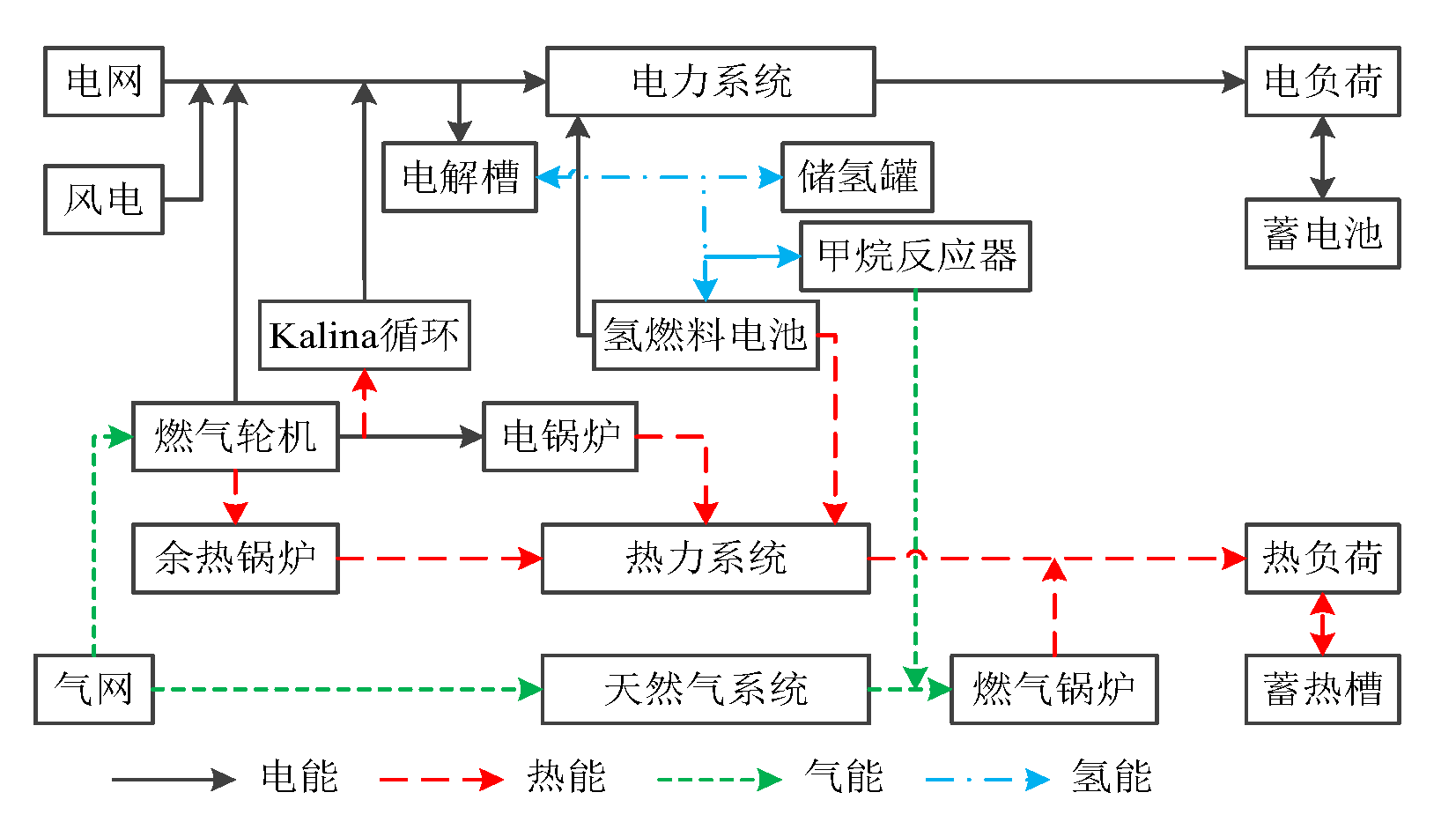
Figure 2.
Electricity, heat load and wind power prediction curve.
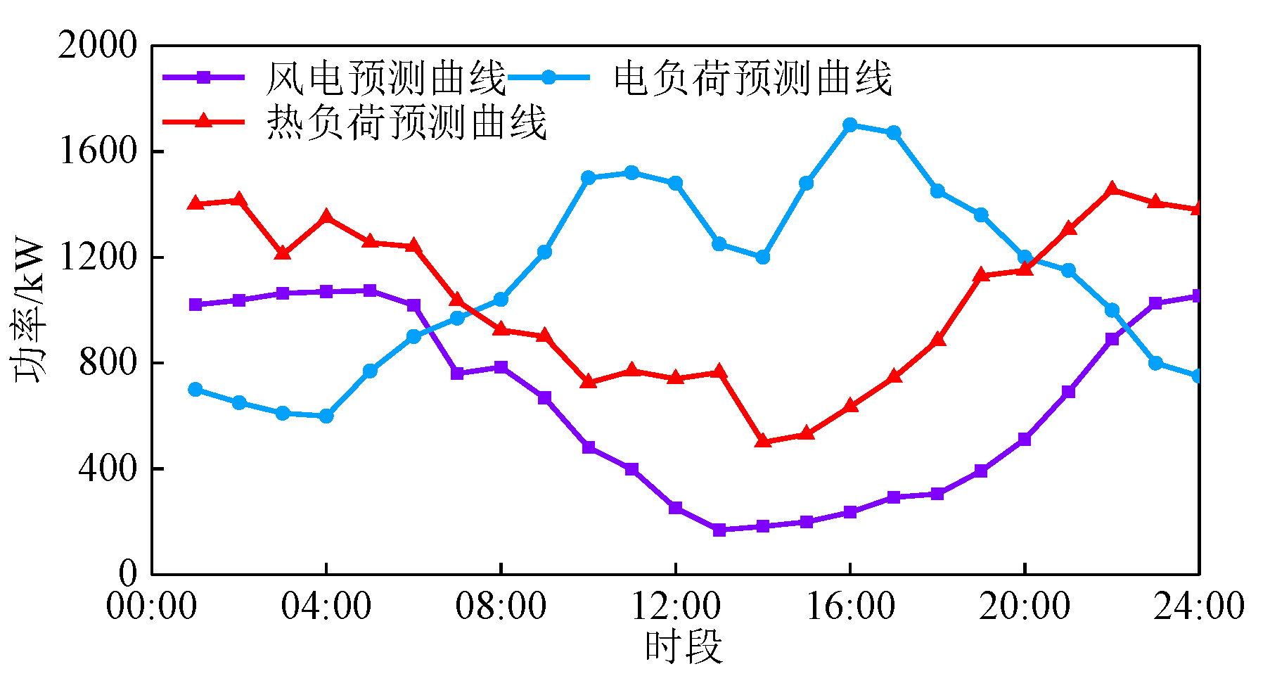
Figure 3.
Typical Daily Outdoor Temperature.
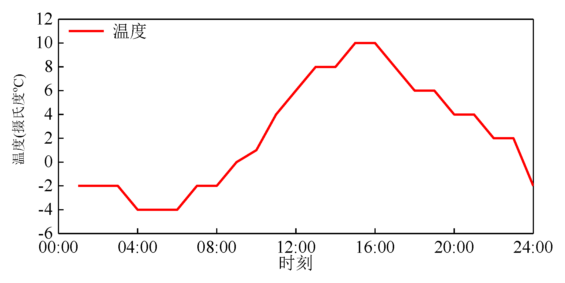
Figure 4.
Wind power consumption results in four scenarios.
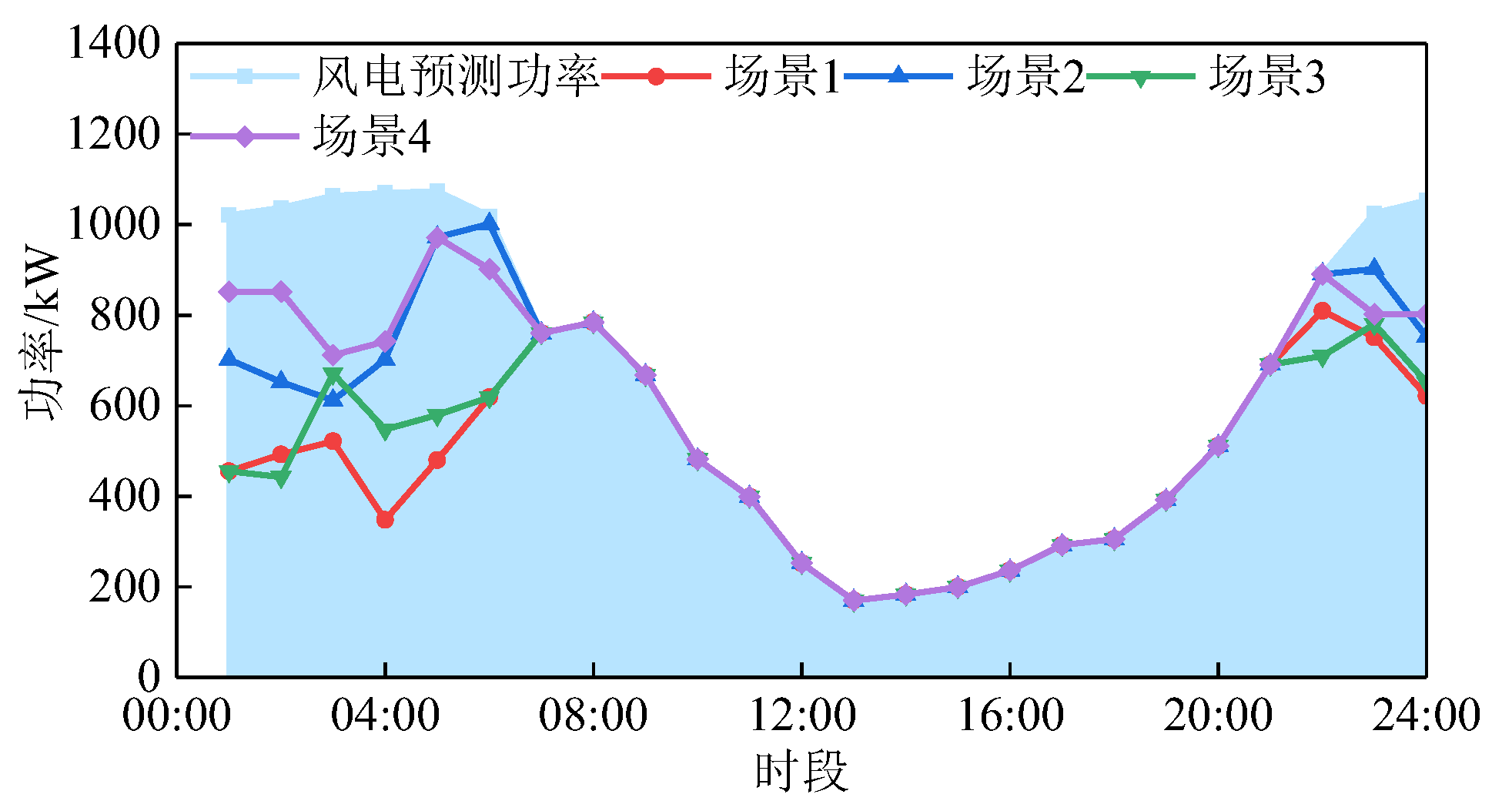
Figure 5.
Decoupling results of cogeneration in four scenarios.
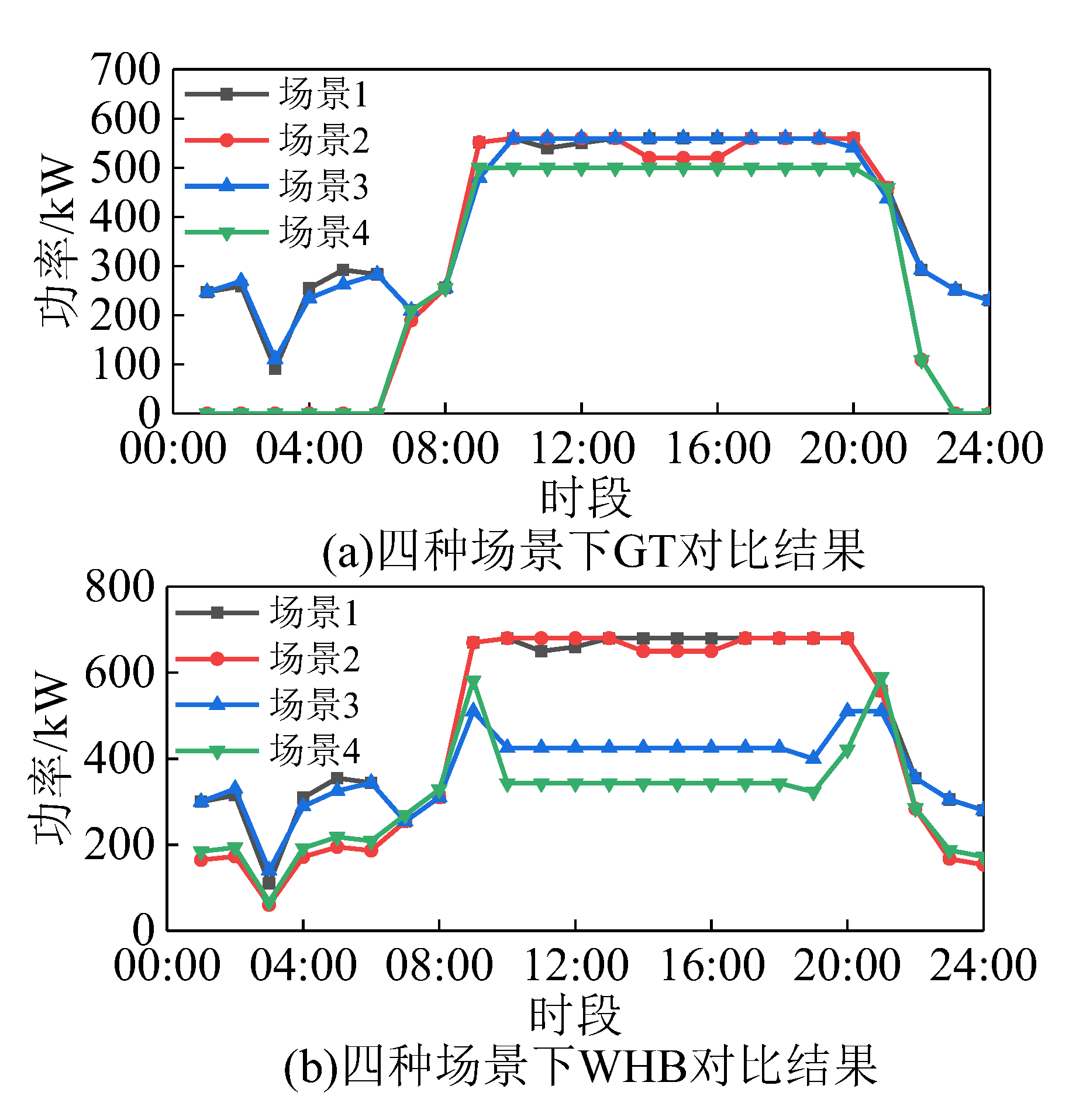
Figure 6.
Electric and thermal power flow direction in scenario 4.
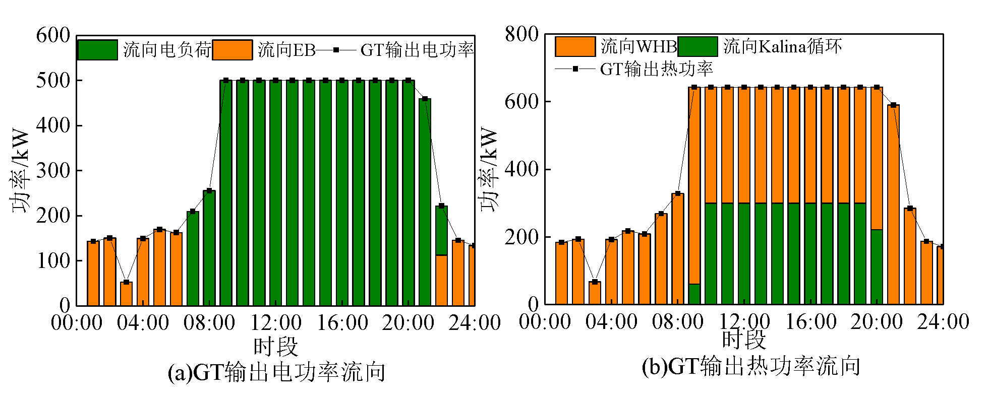
Figure 7.
Electric and thermal power scheduling results for scenario 4.
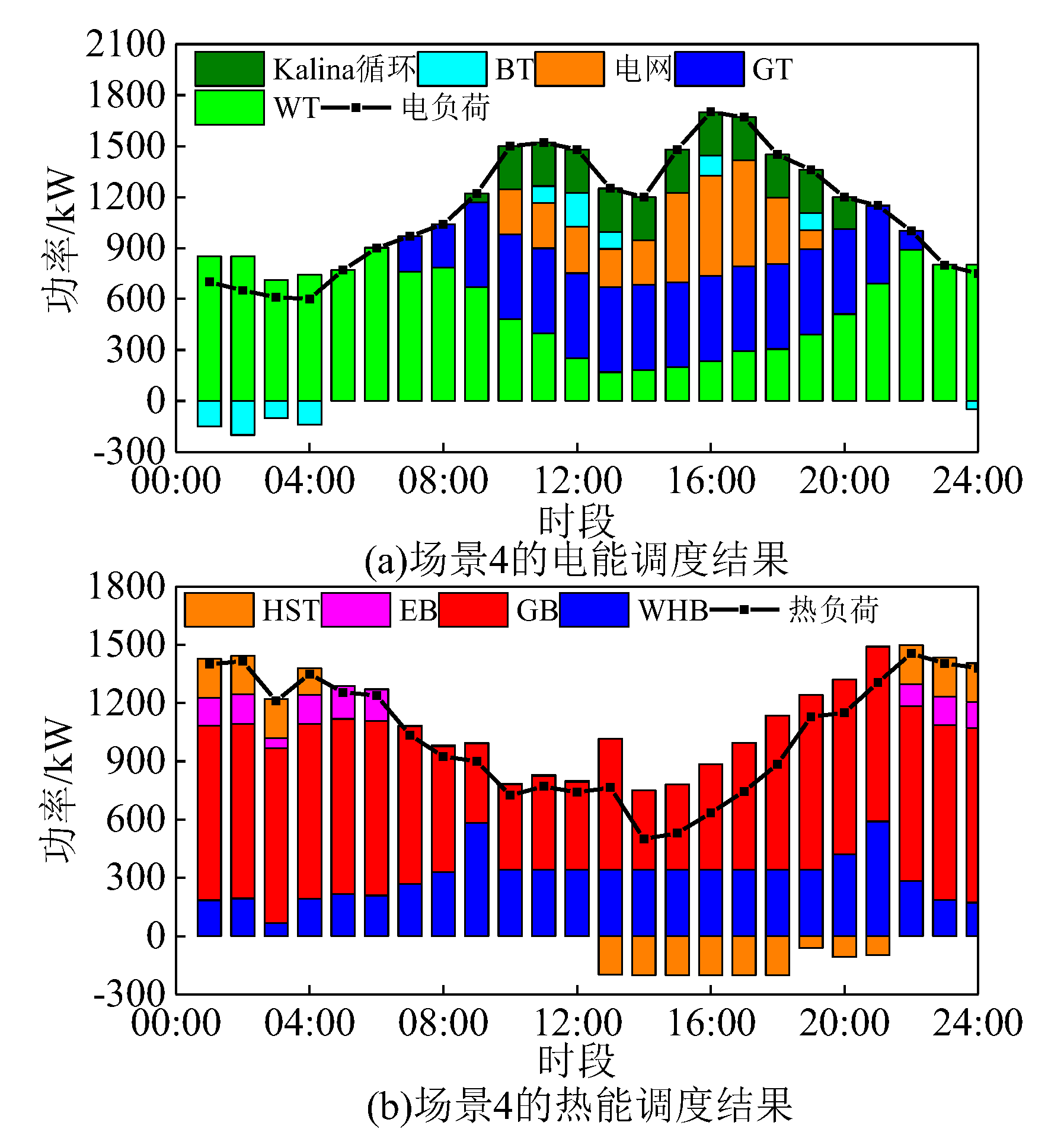
Figure 8.
Comparison results of electric heating Load, wind power, and GT for schemes 1 and 5.
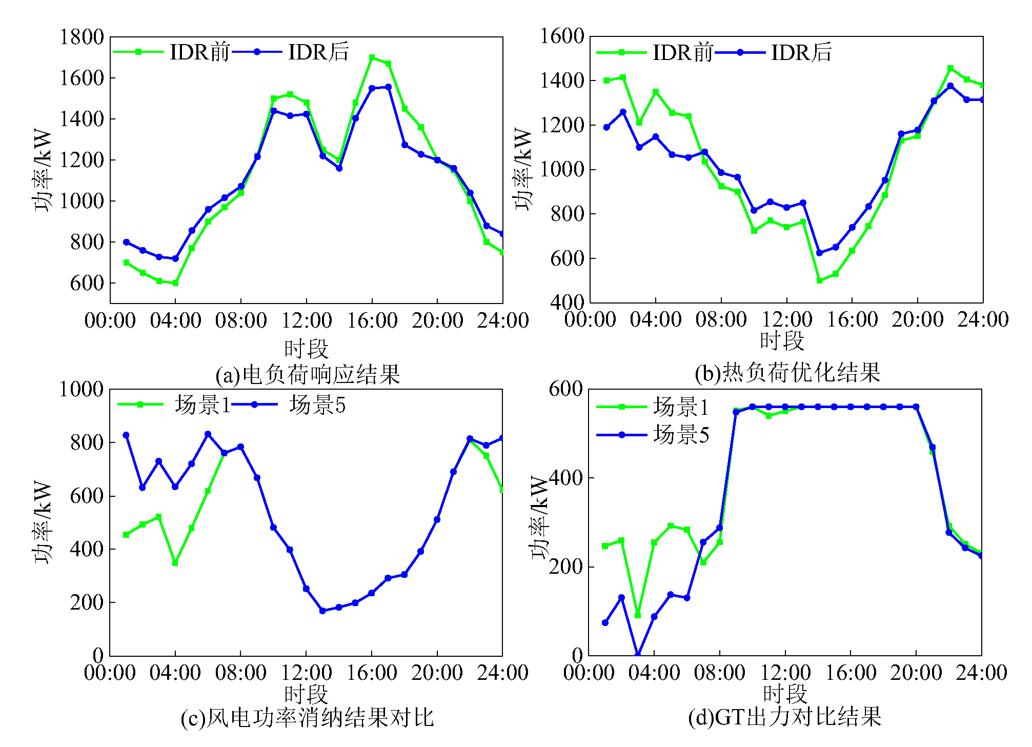
Figure 9.
Comparison of power dispatch results for scenario 6 and wind power consumption results.
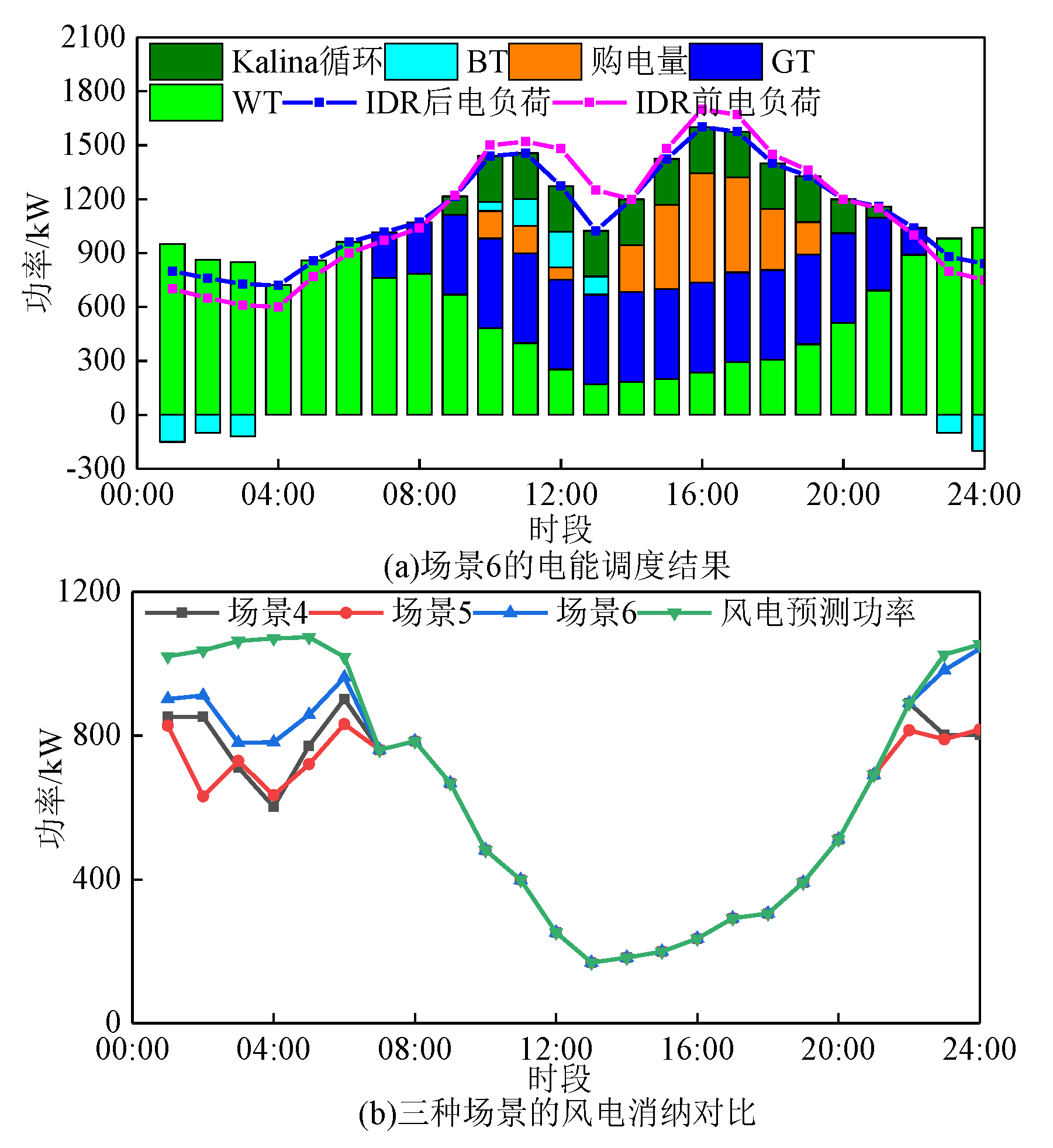

Table 1.
IES’ electricity price parameters.
| Items | Time periods | Yuan/kWh |
| Peak | 08:00-11:00, 17:00-22:00 |
1.21 |
| Off-peak period | 7:00-8:00, 11:00-17:00, 22:00-23:00 | 0.88 |
| Valley | 23:00-24:00,00:00-07:00 | 0.48 |
Table 2.
IES Equipment Parameters.
| Units | Capacity (kW) |
Conversion efficiency | Ramp constraint(kW) | operating cost /(Yuan/kWh) |
| MT | 700 | Power:0.40 Heat:0.50 |
150 | 0.056 |
| Waste Heat Boiler | 800 | 0.85 | 200 | 0.035 |
| Gas Boiler | 800 | 0.9 | 200 | 0.03 |
| EB | 400 | 0.88 | 80 | 0.032 |
| Kalina Cycle | 400 | 0.75 | 80 | 0.06 |
| Electrolyzer | 300 | 0.9 | 60 | 0.048 |
| Methane Reactor | 150 | 0.7 | 30 | 0.055 |
| Hydrogen Storage Tank | 150 | 0.92 | 30 | 0.018 |
Table 3.
Cost results under four schemes.
| Scenarios | C1/ | C2/¥ | C3/¥ | C4/¥ | Total Cost/¥ | Carbon Emissions/kg |
| 1 | 21091.7 | -1131.4 | 3185.6 | 1247.3 | 24393.2 | 11785.8 |
| 2 | 20112.6 | -884.1 | 3311.5 | 826.9 | 23376.9 | 11335.9 |
| 3 | 19974.3 | -1395.6 | 3533.5 | 1164.3 | 23276.5 | 10922.8 |
| 4 | 19628.9 | -1527.0 | 3643.1 | 620.2 | 22365.2 | 10520.4 |
Table 4.
Comparison results between Scenario 1 and Scenario 5.
| Scenario | C1/¥ | C2/¥ | C3/¥ | C4/¥ | Total cost/¥ | Carbon Emissions/kg |
| 1 | 21091.4 | -1131.4 | 3185.6 | 1247.3 | 24393.2 | 11785.8 |
| 5 | 19665.1 | -1253.1 | 3099.6 | 737.1 | 22248.7 | 10497.4 |
Table 5.
Cost comparison results of three schemes.
| Parameters | Scenario 6 | Scenario 7 | Scenario 8 |
| C1 /Yuan | 18673.1 | 17931.4 | 17457.9 |
| C2 /Yuan | 3500.8 | 3813.6 | 3890.9 |
| C3 /Yuan | 391.3 | 0 | 0 |
| C4 /Yuan | -1760.6 | -1945.3 | -1964.1 |
| Total Cost /Yuan | 20804.6 | 19799.7 | 19403.7 |
| Total Carbon Emissions /kg | 9397.5 | 8408.4 | 8179.7 |
Disclaimer/Publisher’s Note: The statements, opinions and data contained in all publications are solely those of the individual author(s) and contributor(s) and not of MDPI and/or the editor(s). MDPI and/or the editor(s) disclaim responsibility for any injury to people or property resulting from any ideas, methods, instructions or products referred to in the content. |
© 2024 by the authors. Licensee MDPI, Basel, Switzerland. This article is an open access article distributed under the terms and conditions of the Creative Commons Attribution (CC BY) license (http://creativecommons.org/licenses/by/4.0/).
Copyright: This open access article is published under a Creative Commons CC BY 4.0 license, which permit the free download, distribution, and reuse, provided that the author and preprint are cited in any reuse.


