
Submitted:
17 August 2025
Posted:
27 August 2025
You are already at the latest version
Abstract
Background
Between-trial heterogeneity is a key element in meta-analysis, traditionally quantified using the I² statistic in studies with binary outcomes. However, survival meta-analyses present additional challenges, as outcomes are usually reported through Kaplan–Meier curves and hazard ratios (HRs). Standard methods for heterogeneity estimation in this context remain poorly established, and consensus is lacking.
Methods
We propose a standardized approach for estimating between-trial heterogeneity in survival meta-analyses using I². The method is applicable both when individual patient data (IPD) are available (collaborative meta-analyses) and when IPD must be reconstructed from published Kaplan–Meier curves (IPDfromKM algorithm). To illustrate the approach, we re-analyzed a published meta-analysis of randomized controlled trials (RCTs) evaluating PARP inhibitor maintenance therapy in extensive-stage small-cell lung cancer. Five RCTs were included, and overall survival was the endpoint.
Results
The binary meta-analysis of crude survival rates yielded no significant heterogeneity (I² = 0%). By contrast, re-analysis based on reconstructed IPD and log-transformed HRs indicated moderate heterogeneity (I² = 36.3%, τ² = 0.0233, p = 0.179). Estimates of the overall treatment effect were similar between approaches (HR ≈ 1.03–1.04), though confidence intervals differed due to model specifications. Comparative evaluation with other methods (Wald test, likelihood ratio, concordance index) highlighted the unique interpretative advantages of I² in this setting.
Discussion
Our findings suggest that crude binary analyses may underestimate heterogeneity in survival meta-analyses. The I² statistic provides an intuitive and flexible measure of between-trial variability when survival data are expressed as HRs. While promising, this approach requires further validation across diverse clinical settings.
Keywords:
meta-analysis
; heterogeneity
; IPDfromKm
; Kaplan-Meier curves
; I-squared
1. Introduction
Most of the meta-analyses published thus far have focused on comparative clinical trials based on binary endpoints, comparing treatment and control groups. In these cases, the typical tool for reporting meta-analytic results is the Forest plot, where trial-specific outcomes are reported alongside a summary measure (e.g. the overall effect). In a forest plot, the degree of between-trial heterogeneity is most often quantified using the I² parameter (expressed as a percentage and associated with a p-value). When the p-value is less than 0.05, the level of between-trial heterogeneity is considered statistically significant [1].
Conversely, the methodology for estimating between-trial heterogeneity in survival meta-analyses is much less standardized. In these cases, the included clinical trials report the outcomes of each arm as a binary time-to-event endpoint. Therefore, these trials take into account both the occurrence of events and the time at which they occurred. Kaplan–Meier plots graphically present the results of these trials, with each trial typically including two curves: one for the treatment arm and the other for the control arm.
There are two types of survival meta-analysis. In the first type (Case 1), researchers conducting the meta-analysis must obtain the individual patient data used to generate the Kaplan-Meier curves through a multicenter collaboration. Specifically, they must receive the original database of individual patient data from the authors of each trial. In the second type (Case 2), researchers examine the published plot of the Kaplan-Meier curves for each trial (along with any additional information reported in the trial) and use a complex algorithm to generate a database of 'reconstructed' individual patient data. This reconstruction is achieved using various algorithms. The most frequently used algorithm is the IPDfromKM method [2], which essentially relies on artificial intelligence.
This paper describes a standardized method of estimating between-trial heterogeneity in survival meta-analyses using the I² calculation. This method can be used regardless of whether the survival meta-analysis is classified as Case 1 or Case 2, as defined above.
To our knowledge, no paper has yet been published describing the application of the I² estimator to a survival meta-analysis. The most frequently used statistical tests for estimating between-trial heterogeneity are Wald's test and the likelihood ratio test. Our paper attempts to address controversies that have arisen in recent years regarding the estimation of heterogeneity in trials using a time-to-event endpoint where outcomes are expressed as a hazard ratio (HR).
2. Methods
In our article, we present a method for estimating between-trial heterogeneity using a real meta-analytic dataset published by Pratama et al. in January 2025 [3]. This example included six RCTs conducted in patients with extensive-stage SCLC who were treated with first-line chemotherapy and then randomized to receive a PARPI maintenance treatment (veliparib, niraparib or olaparib) or not. Five of the RCTs were suitable for our re-analysis [4-8]. Overall survival was the endpoint of our analysis.
3. Results
3.1. Randomized trial included in the analysis
Table 1 summarizes the main information about these five RCTs. As Pratama et al. performed a traditional binary meta-analysis on these five trials, Table 2 shows the results reported by these authors. We focused in particular on assessing heterogeneity, which yielded the following results (see the 8th row in Table 2 and Figure 3 in Pratama et al.'s paper [3]): chi-square = 3.95, df = 4, p=0.41, I² = 0%; meta-analytic risk ratio = 1.03, 95% CI = 0.92 to 1.15, test for overall effect: Z = 0.53, p=0.60. We assumed these results to be a useful reference when estimating heterogeneity using the log(HR) method. It should be noted that using crude rates of event occurrence simplifies the data examined by the meta-analysis, so it is not surprising to find a value of heterogeneity equal to 0%.
3.2. Reconstruction of individual patient data of OS from Kaplan Meier curves by application of the IPDfrom KM method.
The IPDfromKM method was first described in an article by Liu et al., published in 2022. It was a reinterpretation of the method by Guyot et al. [9], with the advantage that it was based on a simple executable file that was freely available online. The IPDfromKM method can also be run under the R platform.
In brief, the IPDfromKM method comprises two phases that must be run sequentially:
1) Digitalization of the Kaplan-Meier curve: in this phase, the image of the Kaplan-Meier curve is analyzed and converted into a series of 50–100 y vs. x data points (where y is the survival rate, expressed on a scale from 0 to 1, and x is time in follow-up, generally expressed in months). Further information to be input in this phase includes the total number of enrolled patients and the total number of events observed during follow-up, as shown in the Kaplan-Meier graph.
2) Analysis of the curve data points and reconstruction of the best-fit patient database that reproduces a Kaplan-Meier curve as similar as possible to the real curve. This database is generated as an Excel XLS file, in which the first column represents time and the second represents the patient's status at that time. Status = 1 indicates death; status = 0 indicates either loss or right censoring; and status = 0 indicates the patient's last observation during the follow-up.
Further details about these two operational phases can be found in numerous articles, many of which were written by our group. In these publications, the IPDfromKM method has been shown to produce high-quality databases of reconstructed patients. The main limitation of the method is that, by definition, the information obtained from the Kaplan–Meier curve is univariate, based on the selected time-to-event endpoint (usually overall survival, recurrence-free survival or progression-free survival).
3.3. Estimation of between-trial heterogeneity from individual patient data of the 5 trials reconstructed from Kaplan-Meier curves: description of the previous method
Table 4 and Figure 1 summarize the results generated by our analysis based on “reconstructed” patients.

Table 3.
Reanalysis of the 5 trials performed by reconstruction of individual patient data (IPDfromKM method).
Table 3.
Reanalysis of the 5 trials performed by reconstruction of individual patient data (IPDfromKM method).
| First author and reference | Experimental group | Control group | Maintenance therapy | Standard treatment | |
| Ai et al. [4] | 48/125 | 22/60 | Xxxx | Xxxx | |
| Byers et al. [5] §§ | 50/61 | 41/61 | xxxx | xxxx | |
| Owonikoko et al. [6] | 52/64 | 54/64 | veliparib+CE | Xxxx | |
| Pietanza et al. [7] | 46/55 | 39/49 | veliparib | xxxx | |
| Woll et al. [8] §§§ | 64§§§/73 olaparib TDS |
59§§§/73 olaparib BD |
60§/74 placebo |
olaparib | placebo |
§ This trial included a third group of 59 patients and 45 deaths, who were treated with veliparib combination. Given that Parama et al. left this trial out of their meta-analysis, our analysis has aligned with this decision and therefore has not included the third arm of this trial. §§ In our IPDfromKM metanalysis, the two Km curves of the two experimental groups were fitted separately to the survival model and then the two groups were summed up at the level of individual patient data; on the contrary, in the binary meta-analysis by Parama et al. the two crude rates were directly summed up to yield a cumulative crude rate. §§§ From the analysis of this trial, a marked difference can be found between how the OS outcomes were managed between the binary metanalysis of Parama et al. [3] and our IPDfromKM meta-analysis based on reconstructed individual patient data; the first found much lower death rates (48/146 in the experimental group vs 25/74 in the controls) because these rates were determined at 12 months; the second found much higher death rates (64/73 in the experimental group vs 59/73 in the controls) because the whole KM curves were analyzed up to 24 months. Abbreviations: TDS, three times daily; BD, twice daily.
Table 4.
Comparison of study-specific results and meta-analytic results between the binary meta-analysis of Pratama et al. and those generated by our IPDfromKm meta-analysis.
Table 4.
Comparison of study-specific results and meta-analytic results between the binary meta-analysis of Pratama et al. and those generated by our IPDfromKm meta-analysis.
| . | ||
| Original RCT | Adjusted values of HR reported in the original trial§ | HR estimated from “reconstructed patients”§. |
| Ai et al. [4] | 1.03 (95%CI, 0.62 to 1.73), p=0.90 | 1.359 (95%CI, 0.8623 to 2.143), p=0.186 |
| Byers et al. [5] | 1.460 (80% CI, 1.104 to 1.931†), p=0.083 | 1.483 (95%CI, 0.9657 to 2.278†), p=0.072) |
| Owonikoko et al. [6] | 0.83 (80% CI, 0.64 to 1.07†), p=0.34 | 0.864 (95%CI, 0.5857 to 1.275†), p=0.461 |
| Pietanza et al. [7] | NR | 0.8578 (95%CI, 0.557 to 1.321), p=0.487 |
| Woll et al. [8] |
-Split HR:§§ 1) 0.85 (90%CI, 0.63, 1.15; p=0.376) 2) 1.03 (90%CI, 0.77, 1.39; p=0.85) -Pooled HR: NR |
- Split HR:§§ 1) 0.8587 (95%CI, 0.603 1.222), p=0.398 2) 1.036 (95%CI, 0.7228 to 1.484), p=0.849 -Pooled HR: 0.9102 (95%CI, 0.668 to 1.2399), p=0.551 |
| Overall effect | 1.03, 95%CI, 0.92 to 1.15, test for overall effect: Z=0.53, P=0.60. | 1.04, 95%CI: 0.83 to 1.30, P=0.74 |
| . | ||
§ The values of HR reported in the original trials were estimated by multivariate analysis, while those estimated from reconstructed patients were derived from univariate analysis. †In this case, the CI in the original trial was at 80%, whereas it was at 95% in the analysis from reconstructed patients. §§ Since this RCT included two treatment groups, in the split HR the first value refers to the first treatment group, while the second value refers to the second treatment group, both compared with the control grop. In the pooled HR, the two treatment groups were pooled together and then compared with the control group. Abbreviations: RCT, randomized controlled trial; CI, confidence interval; NR, not reported.
3.4. Estimation of between-trial heterogeneity from individual patient data of the 5 trials reconstructed from Kaplan-Meier curves: description of the I-squared method
For this estimation, the data source is represented by the HR values reported in the third column of Table 4. These values are as follows: 1.359 (95% CI, 0.8623 to 2.143); 1.483 (95% CI, 0.9657 to 2.278); 0.864 (95% CI, 0.5857 to 1.275); 0.8578 (95% CI, 0.557 to 1.321); and 0.9102 (95% CI, 0.668 to 1.2399).
After performing a log transformation, the meta-analysis of these data yielded the following results (Figure 2):
-HR of meta-analysis = 1.04 (95%CI, 0.83 to 1.30).
- Heterogeneity: I² = 36.3%, tau² = 0.0233, p = 0.1790.
The estimates of heterogeneity differed considerably between the two methods, whereas the estimates of the overall effect were similar. More specifically, the binary meta-analysis yielded an almost identical HR value (1.03; 95% CI, 0.92 to 1.15) compared with the IPDfromKM method. The wider 95% CI for HR found by Pratama et al. can be explained by the fact that the authors used a fixed-effects model, whereas ours was a random-effects model.
Table 6 summarizes the main characteristics of I-squared compared with those of other tests employed in previous studies (Wald test, log-likelihood ratio, concordance or C-index). Finally, Appendix A shows the script in R-language that executes the estimation of between-trial heterogeneity based on the worked example described in Table 2; this estimation is the main finding reported in our Results section.
Table 5.
Comparison of the heterogeneity assessments obtained by the methods previously reported in the literature and those generated by the study-specific results and meta-analytic results between the binary meta-analysis of Pratama et al. and those generated by the I-sqared method described in this paper.
| Comparison | Results of the heterogeneity assessment | |
| Previous method | Method proposed herein | |
|
1) Comparison between the five treatment arms pooled together versus the five control arms pooled together: |
Concordance= 0.521 (se = 0.012 ) Likelihood ratio test= 0.67 on 1 df, p=0.4 Wald test = 0.67 on 1 df, p=0.4 |
The reconstructed curves are shown in Figure 1, panel A; the heterogeneity assessment based on the I-square is shown in |
| 2) Comparison between the five treatment arms plotted individually: | Concordance= 0.565 (se = 0.02 ); Likelihood ratio test= 26.7 on 4 df, p=2e-05; Wald test = 24.82 on 4 df, p=5e-05 |
The reconstructed curves are shown in Figure 1, panel B. |
| 3) Comparison between the five control arms plotted individually: | Concordance= 0.59 (se = 0.02 ); Likelihood ratio test= 14.72 on 4 df, p=0.005; Wald test = 14.76 on 4 df, p=0.005 |
The reconstructed curves are shown in Figure 1, panel C. |
§ The values of HR reported in the original trials were estimated by multivariate analysis, while those estimated from reconstructed patients were derived from univariate analysis. †In this case, the CI in the original trial was at 80%, whereas it was at 95% in the analysis from reconstructed patients. §§ Since this RCT included two treatment groups, in the split HR the first value refers to the first treatment group, while the second value refers to the second treatment group, both compared with the control grop. In the pooled hazrd ratio, the two treatment groups were pooled together and then compared with the control group. Abbreviations: RCT, randomized controlled trial; CI, confidence interval; NR, not reported.
Table 6.
Comparison between the four parameters discussed in the article (I², Wald test, log-likelihood ratio, concordance or C-index); the table makes reference to a meta-analysis comparing Treatment A vs. Treatment B.
Table 6.
Comparison between the four parameters discussed in the article (I², Wald test, log-likelihood ratio, concordance or C-index); the table makes reference to a meta-analysis comparing Treatment A vs. Treatment B.
| Parameter | Does the parameter measure the overall effect of A vs B? | Does the parameter measure the between-trial heterogeneity ? | Is the parameter influenced by the overall effect? |
| I² | No | Yes | No |
| Wald test | Yes | No | Yes |
| Log-likelihood ratio§ | No | Yes | No |
| Concordance or C-index | Yes | No | Yes |
§ In estimating heterogeneity, this parameter should be designed to test the presence of heterogeneity (τ² > 0) versus the absence of heterogeneity (τ² = 0).
4. Discussion
Our analysis addresses the complex issue of methods for estimating heterogeneity in meta-analyses based on time-to-event endpoints, often referred to as survival meta-analyses.
These meta-analyses have sometimes been handled with simple crude rate analysis, which should be considered an overly simplistic method. Our worked example shows that the estimate of the overall effect I may be subject to small differences in terms of the overall effect and to much more substantial differences in terms of heterogeneity. Further analyses however are needed to confirm this preliminary finding.
It is important to remember what the I-squared parameter measures in a meta-analysis and what it does not measure. On the one hand, I-squared measures heterogeneity in both treatment and control arms, but it does not measure the overall effect, which is in fact measured by other parameters such as the pooled risk ratio and the pooled HR.
As a practical recommendation for survival meta-analyses, when all treatment arms have received the same therapy and all control arms have also received the same therapy, I-squared is the best parameter for quantifying the heterogeneity of the clinical material. Basically, in these cases, a single comprehensive analysis of both arms of all included studies is sufficient to acceptably quantify the degree of heterogeneity of the clinical material.
When, on the other hand, the treatment arms have received different treatments while the controls have all been treated in the same way, I-squared is not ideal because it is likely that the different treatments have produced Kaplan-Meier curves that cannot be superimposed. In this case, I-squared is only meaningful when there is no heterogeneity; when it is present and statistically significant, I-squared is not very informative because it is not possible to distinguish between cases where the results were better because the treatment was more effective and cases where certain treatment arms showed better outcomes because the patients enrolled had better prognostic characteristics at enrolment, even though the treatment they received was not more effective.
In conclusion, when the treatments included in the survival meta-analysis are different [9], the 'vertical comparison' approach between all control arms included in the meta-analysis, which many recently published studies have adopted, remains valid. However, further research is needed to establish which heterogeneity parameter is preferable when the assessment of heterogeneity is limited to control arms.
Appendix A. Script in R-language that executes the estimation of between trial heterogeneity based on the worked example shown in Table 2.
|
install.packages("meta") library(meta) # Input of HRs with their respective 95%CI: studi <- c("Studio 1", "Studio 2", "Studio 3", "Studio 4", "Studio 5") HR <- c(1.359, 1.483, 0.864, 0.8578, 0.9102) lower_CI <- c(0.8623, 0.9657, 0.5857, 0.557, 0.668) upper_CI <- c(2.143, 2.278, 1.275, 1.321, 1.2399) # Running the meta-analysis meta_HR <- metagen( TE = log(HR), # log(HR) lower = log(lower_CI), # log(Lower CI) upper = log(upper_CI), # log(Upper CI) studlab = studi, sm = "HR", # hazard ratio comb.fixed = FALSE, # random-effects model comb.random = TRUE, method.tau = "DL" # DerSimonian-Laird method for estimating tau-squared ) # Main results print(meta_HR) forest(meta_HR) |
References
- Higgins JP, Thompson SG. Quantifying heterogeneity in a meta-analysis. Stat Med. 2002 Jun 15;21(11):1539-58. PMID: 12111919. [CrossRef]
- Liu N, Zhou Y, Lee JJ. IPDfromKM: reconstruct individual patient data from published Kaplan-Meier survival curves. BMC Med Res Methodol. 2021 Jun 1;21(1):111. PMID: 34074267; PMCID: PMC8168323. [CrossRef]
- Pratama S, Wiyono L, Setiawan MS, Lauren BC. PARP inhibitors as therapy for small cell lung carcinoma: A systematic review and meta-analysis of clinical trials. Cancer Treat Res Commun. 2024;42:100874. Epub 2025 Jan 27. PMID: 39892078. [CrossRef]
- Ai X, Y Pan, J Shi, et al., Efficacy and safety of niraparib as maintenance treatment in patients with extensive-stage SCLC after first-line chemotherapy: a randomized, double-blind, phase 3 study, J. Thorac. Oncol. 16 (8) (2021) 1403–1414. [CrossRef]
- Byers LA, D Bentsion, S Gans, et al., Veliparib in combination with carboplatin and etoposide in patients with treatment-naïve extensive-stage small cell lung cancer: a phase 2 randomized study, Clin. Cancer Res. Off J. Am. Assoc. Cancer Res 27 (14) (2021) 3884–3895. [CrossRef]
- Owonikoko TK, SE Dahlberg, GL Sica, et al., Randomized phase II trial of cisplatin and etoposide in combination with veliparib or placebo for extensive-stage small-cell lung cancer: ECOG-ACRIN 2511 study, J. Clin. Oncol. 37 (3) (2019) 222–229. [CrossRef]
- Pietanza MC, SN Waqar, LM Krug, et al. Randomized, double-blind, phase II study of temozolomide in combination with either veliparib or placebo in patients with relapsed-sensitive or refractory small-cell lung cancer, J. Clin. Oncol. 36 (23) (2018) 2386–2394. [CrossRef]
- Woll P, P Gaunt, S Danson, et al., Olaparib as maintenance treatment in patients with chemosensitive small cell lung cancer (STOMP): A randomised, double-blind, placebo-controlled phase II trial, Lung Cancer Amst. Neth 171 (2022) 26–33. [CrossRef]
- Hemming K, Hughes JP, McKenzie JE, Forbes AB. Extending the I-squared statistic to describe treatment effect heterogeneity in cluster, multi-centre randomized trials and individual patient data meta-analysis. Stat Methods Med Res. 2021 Feb;30(2):376-395. Epub 2020 Sep 21. PMID: 32955403; PMCID: PMC8173367. [CrossRef]
Figure 1.
Kaplan-Meier curves employed in the heterogeneity assessment based on the method used so far by our research group. Panel A: all treatment groups pooled together versus all control groups pooled together; Panel B: individual curves of the 5 treatment groups compared with one another; Panel C: individual curves of the 5 control groups compared with one another.

Figure 2.
Estimation of heterogeneity through the analysis of HR values and the subsequent estimation of I-squared; these values are those obtained from “reconstructed” patients.
Figure 2.
Estimation of heterogeneity through the analysis of HR values and the subsequent estimation of I-squared; these values are those obtained from “reconstructed” patients.
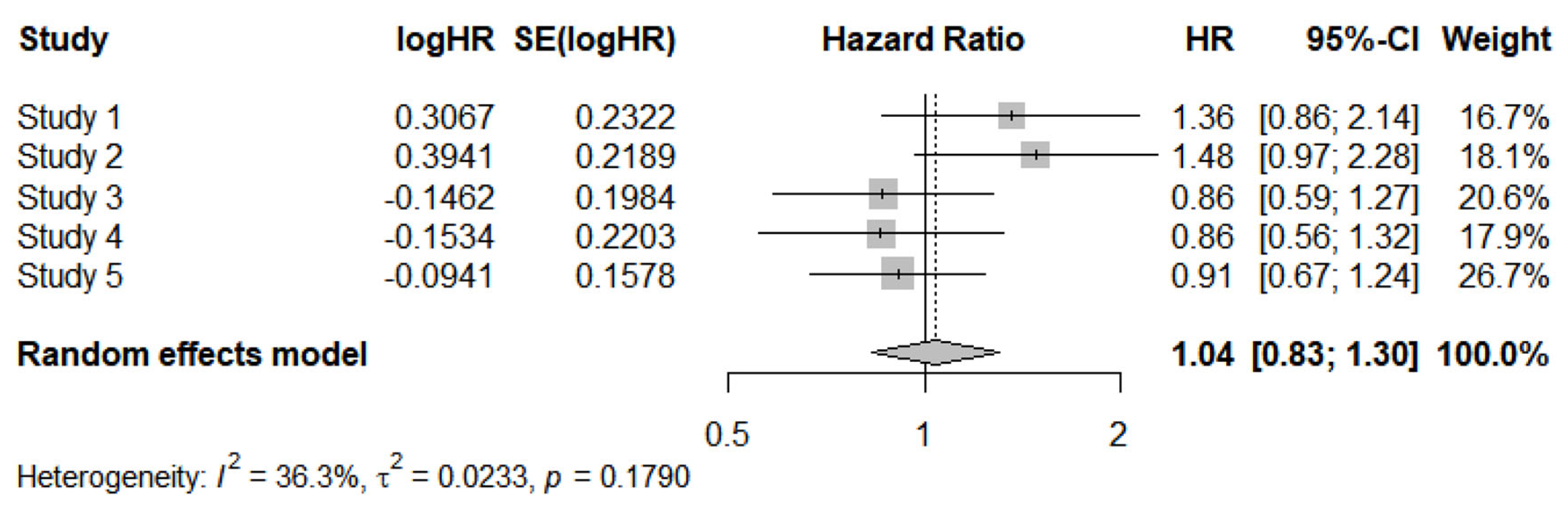
Table 1.
Main information about the 5 included trials.
| First author and reference | Experimental group(s) | Control group | Maintenance therapy | Standard treatment | |
| Ai et al. [4] | 125 | 60 | Niraparib | ||
| Byers et al. [5] | 61 throughout |
59 Veliparib combination |
61 | Veliparib | |
| Owonikoko et al. [6] | 64 | 64 | Veliparib | CE | |
| Pietanza et al. [7] | 55 | 49 | veliparib | ||
| Woll et al. [8] | 73 Olaparib TDS |
73 Olaparib BD |
74 placebo |
Olaparib TDS or Olaparib BD | |
§ The number of events in these three patient groups was not explicitly reported in the original trial; therefore the information shown in this Table was obtained from the database of recontructed patients generated by the IPDfromKM method.
Table 2.
Traditional binary meta-analysis of the 5 trials based on crude death rates; the events is death and overall survival is the end-point.
Table 2.
Traditional binary meta-analysis of the 5 trials based on crude death rates; the events is death and overall survival is the end-point.
| Study | PARPI | Placebo | Risk ratio | ||||
| Events | Total | Events | Total | Risk ratio | Lower 95%CI | Upper 95%CI | |
| Ai 2021 | 48 | 125 | 22 | 60 | 1.05 | 0.70 | 1.96 |
| Byers 2021 § | 50 | 61 | 41 | 61 | 1.22 | 0.99 | 1.51 |
| Pietanza 2018 | 49 | 55 | 44 | 49 | 0.99 | 0.87 | 1.13 |
| Owonikoko 2019 | 51 | 64 | 54 | 64 | 0.94 | 0.80 | 1.11 |
| Woll 2022 §§ | 48 | 146 | 25 | 74 | 0.97 | 0.66 | 1.44 |
| Metanalysis | 1.03 | 0.92 | 1.15 | ||||
| Total events | 246 | 451 | 186 | 308 | 237 | ||
| Heterogeneity: | Chi-square=3.95, df=4, P=0.41, I-square=0%, Z=0.53, P=0.60 | ||||||
| Test for overall effect | Z = t 1.96, p = 0.05 | ||||||
§ This trial included a third group of 59 who were treated with veliparib combination. As Parama et al. [2] left this trial out of their meta-analysis, our analysis has aligned with this decision and therefore has not include the third arm of this trial. §§ From the analysis of this trial, a marked difference can be found between how the OS outcomes were managed between the binary metanalysis of Pratama et al. [3] and our IPDfromKM meta-analysis based on reconstructed individual patient data; the first found much lower death rates (48/146 in the experimental group vs 25/74 in the controls) because these rates were determined at 12 months; the second found much higher death rates (64/73 in the experimental group vs 59/73 in the controls) because the whole KM curves were analyzed up to 24 months.
Disclaimer/Publisher’s Note: The statements, opinions and data contained in all publications are solely those of the individual author(s) and contributor(s) and not of MDPI and/or the editor(s). MDPI and/or the editor(s) disclaim responsibility for any injury to people or property resulting from any ideas, methods, instructions or products referred to in the content. |
© 2025 by the authors. Licensee MDPI, Basel, Switzerland. This article is an open access article distributed under the terms and conditions of the Creative Commons Attribution (CC BY) license (http://creativecommons.org/licenses/by/4.0/).
Copyright: This open access article is published under a Creative Commons CC BY 4.0 license, which permit the free download, distribution, and reuse, provided that the author and preprint are cited in any reuse.


