Fixed-Effect or Random-Effects Models? How to Choose, Perform, and Interpret Meta-Analyses in Clinical Research

Javier Arredondo Montero

doi:10.20944/preprints202509.0126.v3

Submitted:

21 October 2025

Posted:

22 October 2025

You are already at the latest version

Abstract

Meta-analysis has become central to evidence-based medicine, yet a persistent gap remains between statistical experts and clinicians in understanding the implications of model choice. The distinction between fixed- and random-effects is often dismissed as a technical detail, when in fact it defines the very philosophy of evidence synthesis and must be addressed conceptually, a priori, rather than dictated by heterogeneity statistics. Fixed-effect models provide a conditional inference about the average effect within the included studies, based on the assumption that differences between study estimates are due solely to sampling error. Random-effects models, by contrast, acknowledge that true effects differ across studies, populations, and settings, providing wider but more credible intervals that reflect real-world diversity. This work presents a tutorial designed to explain, in a simple and accessible manner, how to conduct an updated and robust evidence synthesis through real and simulated examples—including clinical scenarios, a worked hypothetical meta-analysis, and re-analyses of published reviews—the tutorial demonstrates how model choice can fundamentally alter conclusions. Results that appear significant under a fixed-effect model may become non-significant when using random-effects methods, due to wider confidence intervals that incorporate between-study heterogeneity. In contrast, prediction intervals reveal the range of effects likely to be observed in practice. Drawing on Cochrane guidance, the discussion highlights current standards, including REML and Paule–Mandel estimators, Hartung–Knapp–Sidik–Jonkman confidence intervals, and the routine use of prediction intervals. By combining conceptual examples with practical applications, the tutorial provides clinicians with an accessible introduction to contemporary meta-analytic methods, promoting more reliable evidence synthesis.

Keywords:

meta-analysis

;

fixed-effect model

;

random-effects model

;

heterogeneity

;

prediction intervals

;

evidence synthesis

;

Cochrane Handbook

Subject:

Medicine and Pharmacology - Clinical Medicine

Introduction

Two meta-analyses based on the same set of studies may still reach markedly different conclusions, and for clinicians this is not a statistical curiosity but a practical interpretive problem. The discrepancy usually reflects a modelling choice that is seldom made explicit: whether the meta-analysis adopts a fixed-effect (conditional) framework, in which inference applies only to the included studies, or a random-effects (unconditional) framework, which targets a broader universe of comparable settings. This distinction is not a minor technicality but defines the scope of inference. A fixed-effect model assumes a single underlying effect and yields a precise estimate conditioned on the specific studies analysed. In contrast, a random-effects model assumes a distribution of true effects and incorporates genuine between-study variability into the pooled estimate.

In practical terms, it is the difference between precision restricted to the observed evidence and generalizability to future settings—a foundational issue in evidence synthesis [1].

The Foundational Question: One True Effect?

The choice between fixed- and random-effects models rests on a foundational question: do we believe that all included studies are estimating a single underlying effect, or do we accept that true effects genuinely differ across settings? [2]

A fixed-effect model adopts the first position. It treats each study as a repeated measurement of the same underlying truth, with any variation attributed solely to sampling error. The resulting pooled estimate therefore represents a conditional inference, valid only for the specific set of studies analysed.

A random-effects model adopts the second position. It assumes that the underlying effects legitimately vary across populations, healthcare environments, or implementation conditions, and that meta-analysis should estimate the mean of a distribution of true effects rather than a single constant value. This yields an unconditional inference, intended to generalize beyond the included sample to a wider “superpopulation” of comparable contexts [3].

A practical analogy helps anchor the distinction. Estimating gravitational acceleration is a fixed-effect problem: there is one physical constant (≈9.81 m/s²), and observed variation reflects only measurement error. Estimating average systolic blood pressure across cities, by contrast, is a random-effects problem: the true mean legitimately differs between cities, and the question is not to find a single constant, but to summarise the distribution of those means and the extent of their dispersion (τ²).

Thus, model choice is not a technical afterthought but a decision about what question we are answering. The fixed-effect model asks, “what was the average effect in these exact studies?”, whereas the random-effects model asks, “what effect should we expect across comparable future settings?”. Table 1 expands this distinction through additional clinical examples illustrating how the inferential target determines interpretation.

Table 1. Illustrative and simplified clinical scenarios contrasting the assumptions of fixed-effect and random-effects models.

Clinical Scenario	Under a fixed-effect framework	Under a fixed-effect framework
In non-operative management of uncomplicated appendicitis (antibiotics alone), is the success rate the same across all hospitals?	Assumes a single common success rate across all included hospitals, with observed variation attributed to sampling error.	Assumes that the pooled result represents the average success rate expected across a wider set of comparable hospitals, reflecting true underlying variation (e.g., due to case selection, imaging protocols, or discharge criteria).
Do ACE inhibitors lower blood pressure by the same amount in every patient?	Assumes a common true reduction (e.g., ~10 mmHg) for all included trials. Variation between reported effects is handled as sampling error around this shared underlying value.	Assumes the true reduction differs across patient populations and settings (e.g., larger in some groups, smaller in others), and the pooled value is the average across this distribution of true effects.
Does screening colonoscopy reduce colorectal cancer mortality equally in all health systems?	Assumes that screening colonoscopy provides the same mortality reduction regardless of context.	Assumes that the pooled estimate represents the average mortality reduction across a broader range of comparable screening programs, with true effects differing between programs (for example, due to differences in resources, coverage, or adenoma detection rates).
Does prone positioning reduce mortality in ARDS patients to the same extent across ICUs?	Assumes a uniform mortality reduction across all settings (e.g., 15%).	Treats differences in mortality effect as true variation between ICUs (e.g., protocolisation, staffing differences), with the pooled estimate representing the mean of these effects.
Do COVID-19 vaccines protect against infection?	Assumes identical vaccine effectiveness across all groups, regardless of age, comorbidity, or circulating variants.	Assumes true VE varies across populations and circumstances (e.g., age, comorbidities, circulating variants), and the pooled estimate is the average across this distribution.
Does a smoking cessation intervention increase quit rates equally across settings?	Assumes that this intervention produces the same improvement in quit rates everywhere, with any observed variation across studies explained only by chance.	Assumes quit rates vary across settings (e.g., greater with intensive behavioural support, lower with minimal support), and the pooled estimate is the mean across these true effects.

ACE = angiotensin-converting enzyme; ARDS = acute respiratory distress syndrome; ICU = intensive care unit; VE: vaccination efficacy.

Table 2. Choosing between fixed and random-effects: a clinician’s guide.

Criterion	Fixed-effect (common-effect) model	Random-effects model
Underlying assumption	Assumes a single true effect applies to all included studies; observed differences are attributed to sampling error.	Assumes true effects differ between studies and the pooled estimate is the mean of this distribution.
Scope of inference	Conditional: inference is restricted to the set of studies actually included in the meta-analysis.	Unconditional: inference targets a broader universe of comparable studies/settings.
Handling of study-level confounding	Robust to stable between-study confounding (measured or unmeasured), because all heterogeneity is conditioned out of the pooled estimate.	Vulnerable to study-level confounding, because the pooled effect averages across settings that may differ systematically in factors correlated with the effect.
Clinical diversity	Appropriate only when the included studies are functionally interchangeable regarding design, population, and context.	Appropriate when real differences exist across studies (patients, implementation, healthcare systems).
Generalizability	Limited to the included studies.	Broader: generalizes to comparable study settings.
Precision	Yields narrower intervals because between-study variance is not modelled.	Yields wider intervals because between-study variance is explicitly incorporated.
Role in practice	Suitable for sensitivity analyses, replication contexts, or intentionally conditional inference.	Preferred as the default approach in clinical meta-analysis when the goal is generalization.

Fixed-Effect Models: Scope and Limitations

Fixed-effect models are appealing because they treat all studies as estimating a single common effect, which produces a pooled estimate with narrow confidence intervals and the impression of high precision. This makes them attractive in practice: they answer a clear question with an apparently definitive number. However, this precision is purely conditional on the included studies. If the true effect legitimately varies across settings, the fixed-effect model does not incorporate this variability and therefore cannot generalize beyond the observed data.

A second reason fixed-effect models are sometimes preferred—especially in non-randomized research—is their robustness to study-level confounding. By conditioning inference on this exact set of studies, the model effectively removes all between-study differences (measured or unmeasured) from the estimand. In that narrow sense, the estimate is “protected” from confounding originating at the study level. But this robustness is obtained by collapsing the target of inference: the result is valid only for these studies, not for future applications or external populations.

Thus, the trade-off is intrinsic, not technical: fixed-effect modelling sacrifices generalizability in exchange for conditional robustness. It answers a different question—“what was the average effect in this specific evidence base?”—rather than the more clinically relevant one, “what effect should we expect in comparable real-world settings?” When the goal of synthesis is to inform practice or policy, this inferential restriction means that fixed-effect cannot be justified post hoc on the grounds of confounding; the model must be chosen a priori based on the intended scope of inference, not on convenience or statistical appearance.

Random-Effects Models: Scope and Limitations

Random-effects models start from a different premise: variation across studies is not random noise but often reflects real differences in underlying effects. They therefore estimate the mean of a distribution of true effects, rather than a single constant, yielding an unconditional inference that generalizes to a wider superpopulation of settings. This aligns with clinical reality, where treatment effects legitimately differ across populations, care environments, and implementation contexts.

Because random-effects modelling incorporates this between-study variability, it typically produces wider confidence intervals. This is not a weakness but a representation of additional uncertainty that fixed-effect models suppress. The wider interval reflects both the sampled studies and the dispersion expected in future, comparable settings.

However, this broader inferential target comes with its own assumption: that the true effects are not correlated with study-level characteristics. When unmeasured confounders are linked to the magnitude of the effect, this assumption is violated, and the pooled estimate may be biased. In that sense, random-effects is more generalizable but less robust to confounding than fixed-effect.

In practice, the random-effects framework captures what clinicians intuitively recognise—that effects differ across patients, institutions, and healthcare systems—and makes this variability explicit in the pooled estimate.

Heterogeneity as the Compass for Model Choice

What Heterogeneity Means

Heterogeneity is the observable fact that study results are not identical [4,5,6,7,8,9]. The relevant question in meta-analysis is not whether variation exists—it almost always does—but what that variation represents: random fluctuation around a single underlying effect, or genuine differences in the true effects across settings.

Clinical vs. Statistical Heterogeneity

Two forms of heterogeneity should be distinguished:

Clinical heterogeneity: real-world variability in who was studied, what was done, or where it was done. These differences are not “errors” but reflections of normal clinical diversity (e.g., different patient profiles, dosages, techniques, or healthcare settings).
Statistical heterogeneity: heterogeneity “put into numbers.” It describes how much the study estimates differ after accounting for sampling error (i.e., the random imprecision that arises simply because each study observes only a finite sample of patients). Indices like Q, I², and τ² express this variance quantitatively.

Quantifying and Interpreting Heterogeneity

There are several common tools, each with a distinct role:

Cochran’s Q: a χ² (chi-squared) test of the null hypothesis that all studies estimate the same true effect [4]. It checks whether observed dispersion exceeds what would be expected by chance. Q has low power with few studies and excessive sensitivity with many; therefore, a non-significant Q should never be interpreted as evidence of homogeneity.
I²: the percentage of total variation explained by real heterogeneity rather than chance [2,5,6]. Values of 25%, 50%, and 75% are often quoted as low, moderate, and high, but these thresholds are arbitrary and context-dependent. I² is only an estimate and can be unstable with few studies, and because it depends on study precision, large datasets can yield high I² even when absolute differences are clinically trivial. For this reason, I² should be interpreted descriptively and should not dictate model choice.
τ² (between-study variance): an absolute measure of how much true effects differ across studies, expressed on the same scale as the effect size [2,7,8]. A τ² close to zero indicates minimal dispersion of true effects; larger τ² values indicate meaningful underlying variability. τ² drives the weights in random-effects models and determines the width of confidence and prediction intervals. However, it quantifies heterogeneity — it does not explain its sources. Explaining heterogeneity requires further investigation (e.g., subgroup analysis or meta-regression).

Choosing an Estimator for τ²

The choice of how to estimate τ² can meaningfully influence the results of a random-effects meta-analysis. Several estimators exist:

DerSimonian–Laird (DL): the traditional, non-iterative estimator derived from Cochran’s Q statistic [10]. Although historically common and still the default in older software, numerous simulation studies have shown that DL is often negatively biased, systematically underestimating the true between-study variance τ², especially when the number of studies is small or when events are rare. This underestimation leads to overly narrow confidence intervals and an inflated Type I error rate.
Restricted Maximum Likelihood (REML): an iterative estimator that is generally more robust. Simulation studies consistently demonstrate that REML yields a less biased estimate of τ² across a wide range of realistic meta-analytic scenarios compared with DL. For this reason, it is now recommended as the default option in many methodological guidelines, including the Cochrane Handbook.
Paule–Mandel (PM): another robust iterative estimator that frequently performs similarly to REML. PM is also considered a superior alternative to DL and is likewise endorsed by Cochrane as an appropriate default when heterogeneity is expected.

Calculating Confidence Intervals (“the CI”)

Once the average effect is estimated, we need to decide how wide the confidence interval should be.

Wald CI: the traditional, straightforward approach; it often produces intervals that look reassuringly precise but can be too narrow, especially when there are few studies or some heterogeneity [2].
Hartung–Knapp–Sidik–Jonkman (HKSJ): a modern method that produces wider and generally more reliable intervals. It is now considered the standard when heterogeneity is present. With very few studies, it can sometimes yield excessively wide (over-conservative) intervals; however, it remains the better option overall, as cautious inference is safer than overconfident conclusions [11,12].
Modified or truncated HKSJ (mHK): a refinement of the HKSJ method, designed to prevent confidence intervals from becoming excessively wide in rare situations—typically when the number of studies is very small, a common scenario in clinical research, or when the between-study variance is close to zero [13].

A key limitation of all random-effects models is the difficulty of accurately estimating the between-study variance, τ², when the number of included studies is small. With fewer than about ten studies, estimates of τ² are typically unstable, highly imprecise, and often biased—sometimes severely so. Some methodologists recommend at least 20–30 studies for a reliably estimated τ², although such sample sizes are rarely available in clinical research. This instability is precisely why modern inference methods—most notably the HKSJ adjustment—are recommended: they explicitly account for the uncertainty in τ², producing wider but more appropriate confidence intervals when evidence is sparse.

Random-effects models all share the same philosophy—accepting variability—but they differ in how cautious they are. DL + Wald often looks neat and “precise” but can be misleading. REML or Paule–Mandel combined with HKSJ intervals are increasingly seen as the safer choices when evidence is sparse or heterogeneous [2].

Model Choice Should Come First (and I² Should not Be Used to Make This Choice)

Model choice must be defined before looking at heterogeneity statistics [2]. The decision is conceptual: do we assume a single underlying effect (fixed-effect, conditional inference) or a distribution of true effects (random-effects, unconditional inference)? Q, I² and τ² describe variability, but they do not determine the inferential target, and therefore cannot dictate the model. Choosing a model reactively based on an I² cutoff is methodologically incorrect.

In applied work, some degree of heterogeneity is expected in almost all clinical meta-analyses. Where the studies are highly consistent, fixed- and random-effects estimates will converge; divergence signals that variability matters. The role of heterogeneity is therefore interpretive rather than diagnostic: it clarifies for whom the result may generalize, not which model should be used.

Prediction Intervals: Looking Beyond Confidence Intervals

Prediction intervals extend inference from “what is the mean effect?” to “what range of effects should we expect in a new but comparable setting?” [3,14,15]. This distinction is clinically important: many meta-analyses remain statistically significant at the CI level, yet their PIs include the null, signalling that the effect is fragile or highly context-dependent — a pattern observed in nearly 75% of re-analysed reviews [16]. PIs can only be computed under a random-effects framework when τ² > 0; when τ² collapses to zero, the model becomes effectively fixed-effect and the CI and PI coincide.

So, Which Model Should I Choose?

Key Principles for Model Choice

The choice of model follows directly from the intended scope of inference. Once the distinction between conditional (fixed-effect) and unconditional (random-effects) inference is understood, model selection becomes straightforward: it should be based on what question the synthesis intends to answer, not on the magnitude of I² or any other heterogeneity statistic. These numbers describe variability but do not determine the philosophical target of the model. The starting question is always: do we assume one underlying effect, or many?

What Cochrane Recommends

Accordingly, the Cochrane Handbook recommends random-effects models as the default whenever clinical diversity is present — which is the norm in most applied meta-analyses [2]. Fixed-effect modelling is defensible only when studies are genuinely homogeneous in design, population, and context, or when used deliberately as a sensitivity analysis to test the stability of results. Switching models reactively based on an I² cutoff remains methodologically unsound. Table 3 reports the explicit recommendations of the Cochrane Handbook on model choice and inference, together with their practical implications for clinical meta-analysis.

Practical Guidance for Clinicians

For clinicians, the practical implication is that random-effects should generally be preferred when the aim is to generalize findings beyond the exact studies included. Fixed-effect analysis remains useful primarily as a sensitivity check, or in the rare circumstance where studies are genuinely homogeneous. If a result is statistically significant under fixed-effect but not under random-effects, this indicates that the observed effect is not stable across settings and that heterogeneity materially affects inference.

Interpretation should therefore begin with the pattern of individual study effects, not the pooled number: if studies point in different directions, a seemingly precise fixed-effect estimate has limited external relevance. The model is not just a technical choice; it determines whether the synthesis speaks only to these studies or to future, comparable settings.

Making It Visual: Fixed vs Random at a Glance

The conceptual contrast between fixed- and random-effects is made explicit in a simulated meta-analysis (Figure 1) of six randomized trials evaluating a hypothetical antithrombotic agent. The dataset is intentionally constructed to mimic a common real-world scenario: all studies point in the same direction (fewer thrombotic events with treatment), but the magnitude of effect varies meaningfully across trials.

Under a fixed-effect Mantel–Haenszel model, pooling these trials yields a statistically significant reduction (RR 0.73, 95% CI 0.62–0.87), which appears to imply a uniform ≈27% benefit across all contexts. When the same dataset is analysed using a random-effects model with REML, the point estimate remains similar but the confidence interval widens (RR 0.76, 95% CI 0.58–0.99), and incorporating the Hartung–Knapp adjustment renders the association non-significant (RR 0.76, 95% CI 0.55–1.05).

The prediction interval makes the implication clinically transparent: 95% PI 0.36–1.57 indicates that in a future but comparable trial, the effect could plausibly range from substantial benefit to no benefit or even harm. This is precisely the aspect the simulation is designed to expose — fixed-effect models create the appearance of a universal effect, whereas random-effects modelling reflects the uncertainty and contextual variability that clinicians should expect when translating evidence into practice.

The heterogeneity observed in this example could plausibly arise from multiple sources: Do all patients across trials share the same baseline thrombotic risk, or were study populations selected differently? Were thrombotic events documented consistently across centers, or did outcome assessment vary? Were prophylaxis protocols strictly adhered to in all trials, or was implementation uneven? These questions illustrate that heterogeneity is not a nuisance but often reflects genuine clinical and methodological differences that need to be acknowledged rather than averaged away.

How to Report a Meta-Analysis

Methods

Transparent reporting requires specifying which model was used, which τ² estimator (e.g., REML, Paule–Mandel, DerSimonian–Laird), and how uncertainty was quantified (e.g., Wald vs. Hartung–Knapp). Software and commands should be reported, as should any pre-specified approaches to exploring heterogeneity (subgroup analysis, sensitivity analysis, or meta-regression). When zero-event studies are present, the continuity correction must also be stated, since different approaches (fixed 0.5 vs. treatment-arm continuity correction) yield meaningfully different estimates.

Pre-specification prevents selective reporting and clarifies the inferential target. Just as reporting the average SBP alone is insufficient without describing the spread of true values, meta-analyses should report both the pooled effect and the dispersion of true effects (τ² and, where applicable, the prediction interval). Adherence to Cochrane guidance [2] and PRISMA 2020 reporting standards [17] ensures reproducibility, interpretability, and methodological transparency.

Results

In the results section, meta-analytic findings should be presented with a forest plot showing individual study effects, the pooled estimate, and heterogeneity statistics (Q, I², τ²). Confidence intervals should be reported for all pooled estimates, and prediction intervals whenever random-effects models are used. The model specification and the method for computing intervals (for example, Wald versus Hartung–Knapp) must be stated explicitly. If continuity corrections were applied, the chosen method and its rationale should also be reported. Transparent presentation of these elements allows readers to judge the robustness and reproducibility of the findings.

Table 4 summarizes the essential elements that should be transparently reported in the methods and results of a meta-analysis, including model choice, heterogeneity measures, confidence and prediction intervals, and sensitivity analyses.

A Practical Workflow for Performing a Meta-Analysis

This section outlines the practical steps involved in fitting a meta-analysis, from data extraction to final inference. The goal is not to teach software syntax, but to make explicit what each modelling decision represents so that the analytical choices reported in the Methods and Results are transparent and interpretable.

Step 1 — Define and Extract the Effect Size

The analyst must first determine which effect measure is appropriate (e.g., log risk ratio, log odds ratio, mean difference, or standardized mean difference) and extract both the estimate and its corresponding sampling variance for each included study. These two quantities—effect size and variance—are the essential inputs required by all meta-analytic models.

Step 2 — Specify the Modelling Framework

Before looking at heterogeneity statistics, a conceptual decision is made between a fixed-effect model (assuming a single underlying true effect) or a random-effects model (assuming a distribution of true effects across studies). This is a philosophical choice about the target of inference, not a reactive decision based on I² or Q.

Step 3 — Choose How Between-Study Heterogeneity Is Estimated

Under random-effects, a τ² estimator must be selected. Contemporary methodological guidance recommends REML or Paule–Mandel because they yield more stable and less biased estimates than the traditional DerSimonian–Laird estimator, particularly when few studies are available or effects are heterogeneous.

Step 4 — Choose How Uncertainty Is Quantified

Once the pooled estimate is obtained, the analyst must select a confidence interval method. Wald intervals often appear narrow but can be misleading. Modern guidance recommends Hartung–Knapp–Sidik–Jonkman, which better reflects real uncertainty, especially with small evidence bases.

Step 5 — Interpret Heterogeneity

Only after the model is fitted are heterogeneity statistics (τ², I², Q) interpreted. These numbers summarise how much true variability exists between studies—but they do not determine the model itself. Their role is descriptive and interpretive, not decisive.

Step 6 — Report Generalizability via Prediction Intervals

A prediction interval extends inference from “what is the average effect?” to “what range of effects might realistically appear in a future setting?”. This clarifies whether results are broadly applicable or highly context-dependent.

Step 7 — Sensitivity and Transparency

Finally, the analysis should document:

which modelling framework was used (fixed vs random-effects),
which τ² estimator was applied (e.g., REML or Paule–Mandel),
which CI method was used (e.g., Hartung–Knapp),
and whether continuity corrections or other analytical adjustments were required.

These steps together define what it means to “fit” a meta-analysis in practice. They make the workflow explicit and reproducible, bridging the gap between methodological principles and concrete analytical execution.

Real-World Case Studies: How Fixed vs Random-Effects Alter Conclusions

Applied Case Study 1: Urination Stimulation Techniques in Infants

Clean urine collection in non–toilet-trained infants is clinically challenging: invasive methods such as suprapubic aspiration are painful, while urine bags are prone to contamination. Stimulation techniques (e.g., Herreros’ tapping/massage and the Quick-Wee cold gauze method) were developed to trigger reflex voiding in infants under one year. However, the trials evaluating these methods differ in infant age distribution, manoeuvre type and duration, setting, and operational definition of “successful voiding”; therefore, heterogeneity is mechanistically expected, not incidental.

A published meta-analysis pooled three small randomized trials using a fixed-effect Mantel–Haenszel model and reported a statistically significant and apparently precise effect (OR 3.88, 95% CI 2.28–6.60; I² = 72%) [18]. This inference assumes identical efficacy across studies, despite clear clinical diversity. When re-analysed using a random-effects model with REML, the pooled estimate was directionally similar but the interval widened (OR 3.44, 95% CI 1.20–9.88; p = 0.02). Applying the Hartung–Knapp–Sidik–Jonkman adjustment, recommended for small and heterogeneous datasets, produced a much wider interval and loss of nominal significance (OR 3.44, 95% CI 0.34–34.91; p = 0.15) [19].

This shift is not a statistical artefact but a reflection of model philosophy: with k = 3, τ² is estimated with high uncertainty, so Wald intervals understate variability. HKSJ explicitly incorporates that uncertainty into the interval, which is why the result becomes non-significant. The evidence base is therefore fragile, not because the direction changes, but because stability across settings cannot be assumed.

Applied Case Study 2: Musculoskeletal Outcomes After Esophageal Atresia Repair

Repair of esophageal atresia can be performed thoracoscopically (TR) or via open thoracotomy (COR). Long-term musculoskeletal sequelae (scoliosis, rib fusion, scapular winging) are mainly associated with rib-spreading thoracotomies. The trials comparing TR with COR differ in surgeon experience, stage of the thoracoscopic learning curve, follow-up duration, and diagnostic modality (clinical versus imaging), so genuine heterogeneity is expected rather than incidental.

A fixed-effect Mantel–Haenszel analysis reported a statistically significant reduction in musculoskeletal complications with TR (RR 0.35, 95% CI 0.14–0.84) [20]. However, with only four small retrospective studies and moderate inconsistency (I² = 38%), a random-effects model with REML produced wider uncertainty (RR 0.35, 95% CI 0.09–1.36), and the Hartung–Knapp–Sidik–Jonkman adjustment further widened the interval (RR 0.35, 95% CI 0.05–2.36) [21]. As in Case Study 1, the small k leads to imprecise τ² estimation; fixed-effect appears precise only because it suppresses this uncertainty.

This example shows that the FE estimate is conditionally valid but cannot be generalized. Random-effects with HKSJ provides a more realistic and clinically cautious inference when study-level variability is plausible.

Applied Case Study 3: re-Analysis of Psychological Bulletin Meta-Analyses

A large-scale re-analysis by Schmidt et al. examined 68 meta-analyses originally conducted under a fixed-effect framework [22]. Because these datasets came from diverse populations and research settings, the fixed-effect assumption of a single common effect was rarely defensible. When the same meta-analyses were refitted under random-effects models, confidence intervals widened markedly and many associations lost nominal significance. Fixed-effect inference overstated precision by roughly a factor of two on average, creating an illusion of robustness. Only about 3% of cases were compatible with a genuine single-effect structure; in the overwhelming majority, random-effects provided the appropriate inferential target.

Applied Case Study 4: the Rosiglitazone Link with Myocardial Infarction and Cardiac Death

The rosiglitazone controversy illustrates how model choice can reverse interpretation when event rates are low and trial conditions differ. The original meta-analysis by Nissen and Wolski used a fixed-effect framework on the grounds of non-significant homogeneity tests, despite large differences in dose, comparators, follow-up duration and patient populations [23]. Shuster et al. re-analysed the same 48 trials using random-effects methods appropriate for rare events and reached different conclusions: for myocardial infarction, the fixed-effect model suggested a significant increase in risk (RR 1.43), but the random-effects model rendered the finding non-significant (RR 1.51). For cardiac death, the fixed-effect model appeared null (RR 1.64), whereas the random-effects model showed a clear signal of harm (RR 2.37). This example demonstrates that in rare-event settings, fixed-effect pooling can both mask and exaggerate risk depending on the weight of the largest trial, whereas random-effects more accurately reflect uncertainty across diverse trial conditions.

Applied Case Study 5: The Role of Magnesium in Acute Myocardial Infarction

A meta-analysis of 12 randomized trials evaluating intravenous magnesium for acute myocardial infarction reached different conclusions depending on modelling strategy. Under a fixed-effect model, the pooled estimate was null (OR 1.02, 95% CI 0.96–1.08), despite marked heterogeneity driven largely by a single large trial where magnesium was administered late, often after reperfusion. When re-analysed under a random-effects model, the pooled estimate indicated benefit (OR 0.61, 95% CI 0.43–0.87) [24]. Experimental evidence supports a time-dependent mechanism: magnesium is cardioprotective only when given before or at reperfusion, not after. Thus, the heterogeneity here reflects a real effect modifier (timing), not statistical noise. The fixed-effect model was conditionally correct for the included sample, but the random-effects framework captured the clinically meaningful variability that determines whether benefit is observed.

Table 5 summarizes how conclusions shifted in the five real-world case studies when analyses were re-examined under random-effects models, highlighting how methodological choice can transform the apparent certainty and even the direction of evidence.

Taken together, these case studies show that the contrast between fixed- and random-effects results is structural, not cosmetic. Fixed-effect models concentrate most of the weight in the largest or most precise study, which can mask important between-study differences. Random-effects models distribute weight more evenly when variability is present, yielding inference that better reflects how effects differ across clinical settings.

A Final Nuance: Diagnostic Test Accuracy Studies

Model choice differs in diagnostic test accuracy (DTA) meta-analysis because the standard approach is not a simple fixed-versus-random dichotomy but a hierarchical one. Methods such as the bivariate and HSROC models are likelihood-based and incorporate random effects for both sensitivity and specificity, as well as variability in diagnostic thresholds [25,26,27]. In this setting, heterogeneity is treated as intrinsic to diagnostic performance rather than optional, which is why DTA synthesis is almost always framed within a random-effects perspective.

Conclusions

For ease of application, the core principles of this tutorial are summarized in Table 6 as key take-away messages.

Fixed- and random-effects models are not technical alternatives but reflect different inferential targets: fixed-effect provides conditional inference for the included studies, whereas random-effects provides unconditional inference intended to generalize to comparable future settings. The SBP analogy illustrates this distinction: where true means differ across contexts, a distribution is the appropriate estimand, not a single constant.

In most clinical questions, heterogeneity is expected rather than exceptional, which is why random-effects typically aligns better with the goal of informing practice. Fixed-effect remains appropriate when inference is deliberately restricted to the observed evidence or used as a sensitivity analysis. Heterogeneity is not a problem to be eliminated, but a guide to interpretation, helping determine for whom and under what conditions the synthesized effect is likely to hold.

Supplementary Materials

The following supporting information can be downloaded at the website of this paper posted on Preprints.org.

Original work

The manuscript's author declares that it is an original contribution, not previously published.

Informed consent

N/A.

Ethical Statement

This study did not involve human subjects or animals. As only simulated data were used, no ethical approval or informed consent was required.

Data Availability Statement

A simulated dataset was generated exclusively for illustrative purposes to construct the simulated meta-analysis shown in Figure 1. This dataset is provided as Supplementary File 1.

AI Use Disclosure

ChatGPT (OpenAI) was used for linguistic polishing and dataset generation; the author takes full responsibility for the final content

Conflict of interest

There is no conflict of interest or external funding to declare. The author does not have anything to disclose

References

Riley, R.D.; Gates, S.; Neilson, J.; Alfirevic, Z. Statistical methods can be improved within Cochrane pregnancy and childbirth reviews. J Clin Epidemiol. 2011 Jun;64(6):608-18. [CrossRef]
Higgins JPT, Thomas J, Chandler J, Cumpston M, Li T, Page MJ, Welch VA (eds.). Cochrane Handbook for Systematic Reviews of Interventions. Version 6.5 (updated March 2023). Cochrane, 2023.
Riley, R.D.; Higgins, J.P.; Deeks, J.J. Interpretation of random effects meta-analyses. BMJ. 2011;342:d549.
Cochran, W.G. The combination of estimates from different experiments. Biometrics. 1954;10:101–29.
Higgins, J.P.; Thompson, S.G. Quantifying heterogeneity in a meta-analysis. Stat Med. 2002;21:1539–58.
Higgins, J.P.; Thompson, S.G.; Deeks, J.J.; Altman, D.G. Measuring inconsistency in meta-analyses. BMJ. 2003;327:557–60.
Viechtbauer, W. (2005). Bias and Efficiency of Meta-Analytic Variance Estimators in the Random-Effects Model. Journal of Educational and Behavioral Statistics, 30(3), 261-293. (Original work published 2005. [CrossRef]
Veroniki, A.A.; Jackson, D.; Viechtbauer, W.; Bender, R.; Bowden, J.; Knapp, G.; Kuss, O.; Higgins, J.P.; Langan, D.; Salanti, G. Methods to estimate the between-study variance and its uncertainty in meta-analysis. Res Synth Methods. 2016 Mar;7(1):55-79. [CrossRef]
Arredondo Montero, J. Understanding Heterogeneity in Meta-Analysis: A Structured Methodological Tutorial. Preprints 2025, 2025081527. [CrossRef]
DerSimonian, R.; Laird, N. Meta-analysis in clinical trials. Control Clin Trials. 1986;7:177–88.
IntHout, J.; Ioannidis, J.P.; Borm, G.F. The Hartung-Knapp-Sidik-Jonkman method for random effects meta-analysis is straightforward and considerably outperforms the standard DerSimonian-Laird method. BMC Med Res Methodol. 2014;14:25.
Hartung, J.; Knapp, G. A refined method for the meta-analysis of controlled clinical trials with binary outcome. Stat Med. 2001 Dec 30;20(24):3875-89. [CrossRef]
Röver, C.; Knapp, G.; Friede, T. Hartung-Knapp-Sidik-Jonkman approach and its modification for random-effects meta-analysis with few studies. BMC Med Res Methodol. 2015 Nov 14;15:99. [CrossRef]
IntHout, J.; Ioannidis, J.P.; Rovers, M.M.; Goeman, J.J. Plea for routinely presenting prediction intervals in meta-analysis. BMJ Open. 2016 Jul 12;6(7):e010247. . PMID: 27406637; PMCID: PMC4947751. [CrossRef]
Nagashima, K.; Noma, H.; Furukawa, T.A. Prediction intervals for random-effects meta-analysis: A confidence distribution approach. Stat Methods Med Res. 2019 Jun;28(6):1689-1702. [CrossRef]
Siemens, W.; Meerpohl, J.J.; Rohe, M.S.; Buroh, S.; Schwarzer, G.; Becker, G. Reevaluation of statistically significant meta-analyses in advanced cancer patients using the Hartung-Knapp method and prediction intervals-A methodological study. Res Synth Methods. 2022 May;13(3):330-341. [CrossRef]
Page, M.J.; McKenzie, J.E.; Bossuyt, P.M.; Boutron, I.; Hoffmann, T.C.; Mulrow, C.D.; Shamseer, L.; Tetzlaff, J.M.; Akl, E.A.; Brennan, S.E.; Chou, R.; Glanville, J.; Grimshaw, J.M.; Hróbjartsson, A.; Lalu, M.M.; Li, T.; Loder, E.W.; Mayo-Wilson, E.; McDonald, S.; McGuinness, L.A.; Stewart, L.A.; Thomas, J.; Tricco, A.C.; Welch, V.A.; Whiting, P.; Moher, D. The PRISMA 2020 statement: an updated guideline for reporting systematic reviews. BMJ. 2021 Mar 29;372:n71. [CrossRef]
MMolina-Madueño, S. Rodríguez-Cañamero, and J. M. Carmona-Torres, “Urination Stimulation Techniques for Collecting Clean Urine Samples in Infants Under One Year: Systematic Review and Meta-Analysis,” Acta Paediatrica (2025). [CrossRef]
Arredondo Montero, J. Meta-Analytical Choices Matter: How a Significant Result Becomes Non-Significant Under Appropriate Modelling. Acta Paediatr. 2025 Jul 28. [CrossRef]
Azizoglu, M.; Perez Bertolez, S.; Kamci, T.O.; Arslan, S.; Okur, M.H.; Escolino, M.; Esposito, C.; Erdem Sit, T.; Karakas, E.; Mutanen, A.; Muensterer, O.; Lacher, M. Musculoskeletal outcomes following thoracoscopic versus conventional open repair of esophageal atresia: A systematic review and meta-analysis from pediatric surgery meta-analysis (PESMA) study group. J Pediatr Surg. 2025 Jun 27;60(9):162431. [CrossRef]
Arredondo Montero, J. Letter to the editor: Rethinking the use of fixed-effect models in pediatric surgery meta-analyses. J Pediatr Surg. 2025 Aug 8:162509. [CrossRef]
Schmidt, F.L.; Oh, I.S.; Hayes, T.L. Fixed- versus random-effects models in meta-analysis: model properties and an empirical comparison of differences in results. Br J Math Stat Psychol. 2009 Feb;62(Pt 1):97-128. [CrossRef]
Shuster, J.J.; Jones, L.S.; Salmon, D.A. Fixed vs random effects meta-analysis in rare event studies: the rosiglitazone link with myocardial infarction and cardiac death. Stat Med. 2007 Oct 30;26(24):4375-85. [CrossRef]
Woods, K.L.; Abrams, K. The importance of effect mechanism in the design and interpretation of clinical trials: the role of magnesium in acute myocardial infarction. Prog Cardiovasc Dis. 2002 Jan-Feb;44(4):267-74. [CrossRef]
Deeks JJ, Bossuyt PM, Gatsonis C (eds.). Cochrane Handbook for Systematic Reviews of Diagnostic Test Accuracy. Version 2.0. Cochrane, 2023.
Reitsma, J.B.; Glas, A.S.; Rutjes, A.W.; Scholten, R.J.; Bossuyt, P.M.; Zwinderman, A.H. Bivariate analysis of sensitivity and specificity produces informative summary measures in diagnostic reviews. J Clin Epidemiol. 2005 Oct;58(10):982-90. [CrossRef]
Rutter, C.M.; Gatsonis, C.A. A hierarchical regression approach to meta-analysis of diagnostic test accuracy evaluations. Stat Med. 2001 Oct 15;20(19):2865-84. [CrossRef]

Figure 1. Simulated meta-analysis of six randomized trials of a new antithrombotic agent for postoperative thromboprophylaxis. Each study reports the number of thrombotic events in the treatment (novel agent) and control (conventional prophylaxis) groups. The top panel displays the fixed-effect Mantel–Haenszel model (RR 0.73, 95% CI 0.62–0.87, p < 0.01). The middle panel shows the random-effects model using the REML estimator of τ² (RR 0.76, 95% CI 0.58–0.99, p = 0.04), with between-study variance τ² = 0.05, heterogeneity I² = 50.8%, and Q = 10.96 (p = 0.05); Wald confidence intervals are presented. The bottom panel illustrates the random-effects model using REML with Hartung–Knapp adjustment (RR 0.76, 95% CI 0.55–1.05, p = 0.08), where τ² = 0.05, I² = 50.8%, and Q = 10.96 (p = 0.05); confidence intervals are based on the Hartung–Knapp method. For the random-effects models, the 95% prediction interval (0.36–1.57) indicates that the effect in a future study could plausibly range from substantial benefit to no benefit—or even harm, underscoring the importance of model choice in clinical interpretation. All analyses were performed using Stata version 19.0 (StataCorp LLC, College Station, TX, USA), employing the meta package. A small note for readers: if the analyses are replicated under a Mantel–Haenszel fixed-effect model or using the DerSimonian–Laird method, the heterogeneity summaries will be slightly different from the REML-based figures reported here—specifically, Q = 11.06 on 5 degrees of freedom (p = 0.05) and I² = 54.8%. This occurs because Q and its derivative I² are formally defined within a fixed-effect framework, where study weights depend only on within-study variance. When software such as Stata recalculates these indices using random-effects weights (as in REML), the values shift modestly. Conceptually, the “canonical” values are those from the fixed-effect calculation (54.8% here); DL is consistent with this convention because it computes Q using fixed-effect inverse-variance weights.

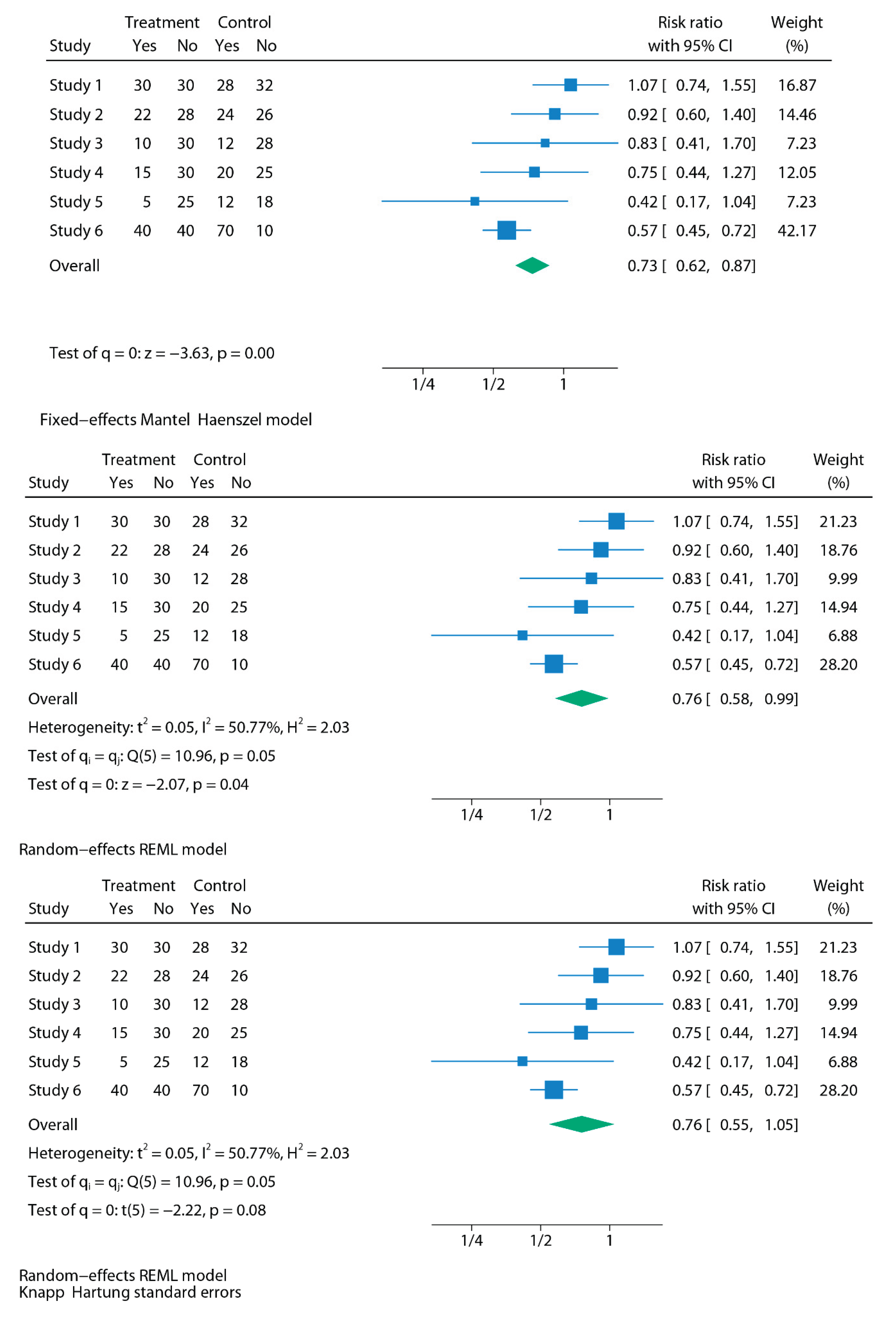
Table 3. Explicit recommendations from the Cochrane Handbook for Systematic Reviews.

Area	Cochrane guidance	Practical implication
Random-effects use	Random-effects models are generally preferred in the presence of clinical diversity (which is the usual situation in clinical research).	Use random-effects as the standard approach, since genuine variability between studies should be assumed unless proven otherwise.
Fixed-effects use	May be appropriate only when studies are truly comparable in design, population, and context.	Restrict fixed-effects to homogeneous data or sensitivity checks.
Role of heterogeneity statistics	Model choice should never be based solely on I² or Q; they are descriptive, not prescriptive. Both I² and Q can be biased, especially when the number of studies is small (which is common in meta-analysis). The most informative metric is τ², as it provides an absolute estimate of between-study variance.	Do not switch models based on I² thresholds. Report τ² as the primary measure of heterogeneity, and interpret I²/Q with caution, particularly in small meta-analyses.
Transparency	Authors should justify their model choice and, when appropriate, report both fixed- and random-effects models.	Present random-effects as primary, fixed-effects as sensitivity.
Confidence Intervals	Wald-type confidence intervals are often too narrow and overconfident, particularly when there are few studies. Hartung–Knapp–Sidik–Jonkman (HKSJ) intervals are recommended, as they provide a more reliable reflection of uncertainty.	Always state which CI method was used in Methods. Prefer HKSJ over Wald, especially with few studies or moderate heterogeneity.
Prediction Intervals	Random-effects analyses should include prediction intervals to reflect the expected range of effects in new studies or settings.	Alongside confidence intervals, report prediction intervals to give clinicians a sense of how treatment effects might vary in practice.
Estimators of heterogeneity	The traditional DerSimonian–Laird estimator is outdated and can underestimate heterogeneity. More robust methods such as Restricted Maximum Likelihood (REML) or Paule–Mandel are recommended.	Use REML by default for τ² estimation, especially when the number of studies is small or heterogeneity is moderate to high.

τ² = between-study variance; I² = inconsistency index; Q = Cochran’s Q test; REML = restricted maximum likelihood; HKSJ = Hartung–Knapp–Sidik–Jonkman.

Table 4. Reporting essentials for a meta-analysis.

Section	What should be reported	Why it matters
Methods	- Pre-registration of the analysis protocol (e.g., in a registry like PROSPERO) -Software and commands used -Rationale for model choice (conceptual justification for using fixed vs random) -Model used (fixed vs random; explicitly report the τ² estimator employed, e.g., REML, Paule–Mandel, or DL) -CI method: explicitly state the procedure used (e.g., Wald, HKSJ, or truncated HKSJ) -Heterogeneity metrics: report Q, I², and τ² together with the τ² estimator used -Strategy to explore heterogeneity (subgroup, sensitivity, meta-regression) -Continuity corrections applied (e.g., 0.5 all-cells correction; treatment-arm continuity correction) -Software limitations (e.g., RevMan 5.4, CMA)	Transparency; reproducibility; avoids selective reporting.
Results	Forest plots that are legible and annotated -Study-level data (e.g., events per group over total) and pooled effects -Heterogeneity metrics: Q, I², τ² -CI 95% (with method specified, e.g., HKSJ) -PI 95% (when random-effects is used)	Ensures clarity; communicates both precision (CI) and expected variability across contexts (PI); readers understand robustness of findings.

τ² = between-study variance; I² = inconsistency index; Q = Cochran’s Q test; CI = confidence interval; PI = prediction interval; DL = DerSimonian–Laird; REML = restricted maximum likelihood; HKSJ = Hartung–Knapp–Sidik–Jonkman; CMA = Comprehensive Meta-Analysis; RevMan = Review Manager.

Table 5. Summary of how conclusions shifted in five real-world case studies when re-analysed under random-effects models.

Case study	Clinical question	Original model & result	Re-analysed model & result	Key lesson
1. Urination stimulation in infants	Non-invasive stimulation to collect urine samples	FE Mantel–Haenszel: OR 3.88 (95% CI 2.28–6.60), p<0.01; I²=72% → strongly positive	RE REML: OR 3.44 (1.20–9.88), p=0.02; HKSJ: OR 3.44 (0.34–34.91), p=0.15 → wide, inconclusive	With k=3, τ² is highly unstable. FE treats heterogeneity as sampling error, whereas RE propagates between-study uncertainty, and HKSJ further widens the interval to reflect small-sample uncertainty.
2. Esophageal atresia repair	Musculoskeletal sequelae after thoracoscopic vs open repair	FE Mantel–Haenszel: RR 0.35 (0.14–0.84), p=0.02 → significant reduction	RE REML: RR 0.35 (0.09–1.36), p=0.13; HKSJ: RR 0.35 (0.05–2.36), p=0.18 → loss of significance	When few retrospective studies are pooled, variance estimation dominates inference. A fixed-effect estimate is conditional on included studies, whereas random-effects shifts the target to a distribution of effects, widening uncertainty.
3. Psychological Bulletin re-analysis	68 psychology meta-analyses re-examined	FE gave narrow, often “significant” CIs; apparent robustness	RE widened CIs, significance often disappeared; FE defensible in ~3% only	Large-scale re-analysis shows that conditional inference under FE is often narrower than the more generalisable unconditional inference under RE.
4. Rosiglitazone & CV risk	Myocardial infarction & cardiac death with rosiglitazone	FE: MI RR 1.43 (1.03–1.98), p=0.03 (↑ risk); cardiac death RR 1.64 (0.98–2.74), p=0.06 (NS)	RE (rare-event): MI RR 1.51 (0.91–2.48), p=0.11 (NS); cardiac death RR 2.37 (1.38–4.07), p=0.0017 (↑ risk)	When event rates are low, and heterogeneity interacts with effect direction, FE weights are dominated by large studies; RE reweights toward distributional heterogeneity, altering inference.
5. Magnesium in acute MI	IV Mg²⁺ for AMI	FE: OR 1.02 (0.96–1.08) → null; extreme heterogeneity (p<0.0001)	RE: OR 0.61 (0.43–0.87), p=0.006 → protective	Heterogeneity here reflects an effect modifier (timing). FE assumes a single underlying effect; RE incorporates clinical variability, allowing the pooled estimate to align with mechanistic context.

FE = fixed-effect; RE = random-effects; REML = restricted maximum likelihood; HKSJ = Hartung–Knapp–Sidik–Jonkman; OR = odds ratio; RR = risk ratio; MI = myocardial infarction; AMI = acute myocardial infarction.

Table 6. Takeaway messages.

Follow Cochrane guidance and the PRISMA 2020 checklist rigorously
Select random-effects models when the goal is unconditional (generalizable) inference
Use fixed-effects models for conditional inference or as a sensitivity analysis
Always report heterogeneity (I², Q, τ²) and include a 95% prediction interval
Use modern methods: apply REML for τ² and HKSJ for confidence intervals
Investigate heterogeneity as a source of clinical information
Report models, estimators, and intervals transparently to ensure reproducibility

Disclaimer/Publisher’s Note: The statements, opinions and data contained in all publications are solely those of the individual author(s) and contributor(s) and not of MDPI and/or the editor(s). MDPI and/or the editor(s) disclaim responsibility for any injury to people or property resulting from any ideas, methods, instructions or products referred to in the content.

© 2025 by the authors. Licensee MDPI, Basel, Switzerland. This article is an open access article distributed under the terms and conditions of the Creative Commons Attribution (CC BY) license (http://creativecommons.org/licenses/by/4.0/).

Copyright: This open access article is published under a Creative Commons CC BY 4.0 license, which permit the free download, distribution, and reuse, provided that the author and preprint are cited in any reuse.