
Submitted:
27 August 2025
Posted:
02 September 2025
You are already at the latest version
Abstract
Meta-analysis is frequently read from the diamond down. The forest plot’s tidy alignment gives the illusion of certainty, with the pooled diamond suggesting a single definitive answer. Yet the forest is rarely uniform: some trunks lean, others twist, and a few tower or collapse, reshaping the skyline. This metaphor illustrates heterogeneity—the unevenness between studies—that ultimately determines the reliability of pooled estimates. This tutorial recenters interpretation on that variability: Q signals its existence, I² describes the proportion beyond chance, and τ² quantifies its magnitude. At the same time, prediction intervals extend these measures into practice by showing the range that future studies may realistically occupy. In diagnostic test accuracy, hierarchical models such as Reitsma’s bivariate and HSROC are highlighted, as they preserve the correlation between sensitivity and specificity and capture threshold-driven heterogeneity. Beyond numerical measures, visual and analytical approaches provide complementary insights into the underlying sources of heterogeneity, helping to explain why studies diverge in their findings. From these tools emerge practical lessons: the need for transparent reporting, robust estimators, prediction intervals, and caution in interpreting subgroup claims, while routine pitfalls—such as defaulting to DerSimonian–Laird, selecting the model solely based on a heterogeneity statistic, or reporting I² in isolation—are avoided. The message is simple: the diamond is not the compass—meta-analysis earns credibility not by multiplying averages, but by explaining the uneven forest behind them.
Keywords:
heterogeneity
; meta-analysis
; Q statistic
; I² statistic
; τ² statistic
; prediction interval
; bivariate meta-analysis
1. Introduction
Imagine walking through two forests. In the first, all trunks stand vertical, of equal height and girth, aligned in neat rows. The skyline is smooth, giving the impression of perfect order. This is homogeneity: studies pointing in the same direction, with slight variation.
Now picture a second forest. Here, one trunk is thicker, another taller, and several lean at different angles. The skyline is uneven and irregular. This is heterogeneity: differences in study results that go beyond what would be expected by chance. In this metaphor, each tree represents a study: its tilt reflects the effect estimate, its height or girth the sample size and precision, and the skyline the pooled evidence. What at first glance may appear to be tidy alignment is, in truth, a landscape of variation—the heterogeneity that ultimately shapes how trustworthy meta-analytic conclusions are (Figure 1).
It is tempting to admire the canopy without a closer look. Meta-analysis invites the same shortcut: our eyes go straight to the diamond at the bottom of the forest plot, the promise of a single answer. But just as the forest is shaped by the tilt and health of individual trees, the pooled estimate is only as meaningful as the variation behind it. Heterogeneity is what lies between the trunks, what bends the landscape, and what can quietly change the story told by the diamond.
Heterogeneity may take on different shapes depending on the type of review—therapeutic, diagnostic, or prognostic. Some forests are dense, while others are sparse; some are tilted by bias or design, while others are shaped by natural diversity. Yet beneath these varied canopies runs the same root system: variability beyond chance, the hidden force that shapes how we should read the forest plot.
Although numerous resources define the statistics used to quantify heterogeneity, there is no unified interpretive guide for practitioners that spans therapeutic, diagnostic, and prognostic reviews while emphasizing modern best practices. This tutorial aims to fill that gap by offering a structured, pedagogical framework anchored in both statistical rigor and clinical relevance.
How is heterogeneity measured?
But how do we measure the irregularities of a forest? One might count trees, compare their heights, or note the angles at which they lean. Each measure captures part of the picture, but none tells the whole story. Meta-analysis is similar: heterogeneity can be quantified in several ways, each with its own strengths and limitations.
The Q statistic
Definition
The Q statistic, introduced by Cochran in 1954 [1], is the oldest test for heterogeneity. It asks whether the differences between study results are larger than expected by chance. In forest terms, a few random tilts are normal, but if several trunks lean sharply in different directions, something real is making the forest uneven. Q distinguishes these scenarios.
In practice, Q sums the squared deviation of each study from the pooled mean, weighting precise studies more strongly. If studies align, Q stays small; if some diverge, Q grows.
Interpretation
Under the null hypothesis of homogeneity, Q follows approximately a chi-square (χ²) distribution with degrees of freedom equal to the number of studies minus one (df = n–1) [2,3]. The χ² distribution may sound intimidating, but it is simply a reference curve for the scatter we would expect by chance. It is like a “null model” of a perfectly straight forest: if the observed Q is much larger than this baseline, the variation is unlikely to be random. Degrees of freedom (df) serve to calibrate this test because they define the χ² curve against which Q is compared when calculating the p-value. In a small grove (with few studies and therefore low df), we expect nearly perfect alignment, so even a single leaning trunk feels alarming. In a vast forest (with numerous studies and thus high df), some tilting is anticipated as part of the baseline variation, and concern arises only when the leaning systematically exceeds this expectation across many trees.
In summary, the higher the Q value, the greater the heterogeneity; the df adjusts the yardstick used to judge whether that value is extreme enough to reject homogeneity. A small p-value (<0.05) suggests real heterogeneity; a large one means the scatter may still be due to chance.
Limitations
Because Q depends directly on df, it is strongly influenced by the number of studies. With few, it has low power and may miss true heterogeneity; with many, it becomes oversensitive, flagging trivial differences [4]. Another key limitation is that Q reflects the amount of excess variation but not its structure. Two meta-analyses can have the same Q value but exhibit very different patterns of irregularity—one with numerous small deviations in height, and another with a single extreme outlier. In forest terms, Q can tell us that the skyline is uneven, but not why: whether the irregularity arises from many trees differing slightly in height, or from a single trunk that is dramatically shorter than the rest (Figure 2). Q is therefore useful as a first signal, but never sufficient on its own.
The I² statistic
Definition.
The I² statistic, introduced by Higgins and Thompson in 2002 [5,6], expresses the proportion of total variability in effect estimates that is due to heterogeneity rather than chance. It is derived from Q and its degrees of freedom (df). I² is a percentage: 0% means all scatter could be random; higher values mean that some of the variation reflects real differences. For example, I² = 50% suggests that half of the observed variability is genuine.
Interpretation.
Guidelines sometimes classify I² values as: 0–40% possibly unimportant, 30–60% moderate, 50–90% substantial, and 75–100% considerable. These thresholds are only rough guides. Two forests may both yield I² = 50% and still look very different: one where tilts are barely noticeable, another where several trunks are almost falling. For this reason, the Cochrane Handbook cautions against applying thresholds rigidly [7].
Limitations.
I² does not measure the actual size of heterogeneity, only its proportion. In meta-analyses involving very precise studies, even small absolute differences can yield high I². Conversely, with small, imprecise studies, I² may appear low despite an obvious spread, or it may overestimate inconsistency due to noise [8]. Another limitation is instability with few studies: with a small forest of only a handful of trees, I² may underestimate or exaggerate the true inconsistency, and its apparent precision is misleading. In summary, I² is a useful indicator of inconsistency, but it does not reveal the actual magnitude of heterogeneity, and it should never be interpreted in isolation.
The τ² statistic
Definition.
The τ² statistic is the main measure of between-study variance in a meta-analysis. Variance, in simple terms, describes how spread out a set of numbers is. If all studies give almost identical results, the variance is close to zero; if results differ widely, the variance is larger. While Q detects whether heterogeneity exists, and I² expresses the proportion of variation beyond chance, τ² quantifies its absolute magnitude, expressed in the same units as the effect size (risk ratios, mean differences, log odds ratios, etc.).
In forest terms: I² may tell you that half the trunks lean because of real conditions, but τ² tells you how much they lean—whether a few degrees or almost toppling over.
Interpretation.
Fixed-effect models assume that all studies estimate the same underlying effect. Any differences are attributed to sampling error, so between-study variance is assumed to be zero, and τ² is not estimated. In forest terms, this model treats every trunk as perfectly straight, and any tilt we see is dismissed as random noise.
Random-effects models, by contrast, acknowledge that true effects may differ across studies because of variations in populations, interventions, or methods. Here, τ² captures the actual variance of these true effects—the average squared distance between them. If τ² = 0, the forest is uniform; as τ² grows, the trunks lean at increasingly different angles.
Estimating τ² is not trivial. Several methods exist:
- DerSimonian–Laird (DL). The most widely known and historically the default [9]. It is simple—plugging the observed Q into a formula—but biased: with few studies or large true heterogeneity, it tends to underestimate τ², pulling values toward zero and giving overly narrow confidence intervals. Given its well-documented biases, the DL estimator should no longer be regarded as the default choice in modern meta-analysis.
- Paule–Mandel. Another estimator that, like REML. Although classical, it improves over DL and is currently accepted as an REML alternative.
- Bayesian estimators. In Bayesian statistics, τ² is not treated as a fixed number but as something uncertain, described by a probability distribution. We start with a prior (what we already know or assume) and update it with the data to get a posterior (what seems plausible after seeing the evidence) [12]. The advantage is that we can make direct probability statements, like “there is a 70% chance that heterogeneity is above a clinically important level.” This approach is flexible, especially when data are scarce, but the results depend on how the prior is chosen, so it must be done transparently.
Once τ² is estimated, it influences not only descriptive statistics but also inference. The Hartung–Knapp–Sidik–Jonkman (HKSJ) adjustment, now recommended by the Cochrane Handbook [7], uses τ² to provide more robust confidence intervals in random-effects models. This correction is particularly important when the number of studies is small, where conventional Wald-type intervals—the default output in software such as RevMan—systematically underestimate uncertainty and give an illusion of precision. HKSJ intervals are typically wider, but they reflect the real instability that arises when between-study variance is nonzero.
A key conceptual point is that τ² and I² are not interchangeable. Two meta-analyses can both report I² = 50%, meaning that half the observed variability is real. But τ² will reveal whether that variability is modest (a few degrees of tilt: an orderly forest) or extreme (trunks leaning at 30–40°: a chaotic woodland). This contrast is illustrated in Figure 3: in both panels, the proportion of leaning trunks is the same (I² = 50%), yet in one, the tilt is barely perceptible while in the other it is dramatic. This shows why τ², not I², determines the real scale of heterogeneity and directly governs the width of pooled confidence intervals, the span of prediction intervals, and the reliability of meta-regression analyses.
Limitations.
τ² is less intuitive than Q or I² because it is expressed on the same scale as the effect size. A τ² of 0.04 may be trivial for a risk ratio but very large for a mean difference in kilograms. The number itself has meaning only relative to the chosen metric. Another limitation is instability with few studies. When the forest has only a handful of trees, τ² can swing wildly depending on the estimator—sometimes suggesting that trunks are almost perfectly aligned, other times that the woodland is chaotic. In forest terms: two woods may both show I² = 50%, but τ² tells you whether the tilts are mild (all trunks leaning just a little, still an orderly skyline) or dramatic (several trunks close to falling, creating real disorder). Finally, τ² is often reported without confidence intervals. Yet its uncertainty can be large, especially in small meta-analyses, and ignoring it risks giving a false sense of certainty. In summary: τ² is harder to read than I², but it is the most structural parameter, because it measures the real size of heterogeneity and directly governs the reliability of pooled results. Because τ² is the foundation for any forward-looking inference, prediction intervals (PIs) represent its most direct clinical extension
Prediction intervals: an extension of τ²
A confidence interval reflects the precision of the pooled effect, but says nothing about what a new study might show. PIs extend τ² by translating between-study variance into a range of plausible effects for future settings [13-15]. Because they incorporate both sampling error and heterogeneity, PIs are almost always wider than CIs.
In forest terms, the CI indicates the precision with which we have measured the average tilt of the trunks, while the PI shows the range of tilts we are likely to encounter as we continue walking deeper into the forest. Clinically, this matters: a pooled risk ratio may look beneficial (CI entirely <1.0), yet the PI can cross the line of no effect, warning that in some contexts the intervention may not work—or could even harm.
Limitations. PIs are fragile when based on a few studies (<10–15), often giving misleading coverage. This fragility arises because the prediction interval is calculated from τ²; when τ² itself is unstable—as inevitably occurs with only a few studies—the prediction interval inherits this instability. This link underscores the central importance of obtaining a robust estimate of τ², since every downstream measure of heterogeneity depends on it
PIs should be viewed as a conceptual tool that illustrates the plausible range of effects, rather than a statistically robust interval in small meta-analyses.
Which statistic matters most: Q, I², or τ²?
No single statistic can capture the full complexity of heterogeneity. Q tells us whether the variability across studies exceeds what chance alone would explain. I² expresses what proportion of the observed scatter is real rather than random. τ² measures the absolute magnitude of that variability on the scale of the chosen effect size.
Of these, τ² is the most structural parameter. It directly governs the width of pooled confidence intervals, the span of prediction intervals, and the performance of meta-regression. I² is easy to report and widely recognized, but it is scale-dependent and unstable when only a few studies are available. Q provides a formal test, but it is driven by sample size and degrees of freedom rather than by the actual importance of heterogeneity.
In forest terms: Q asks if the woodland looks unusual, I² tells what fraction of trunks are leaning beyond chance, and τ² measures how far they actually tilt. For interpretation, this means Q and I² are useful signals, but τ²—together with prediction intervals—is the key to understanding what heterogeneity really means for practice.
|
But do these conventional metrics of heterogeneity apply equally to diagnostic accuracy studies? In therapeutic meta-analysis, heterogeneity is typically unidimensional, as all studies estimate the same type of effect. Diagnostic test accuracy (DTA) is different. Here, two outcomes—sensitivity and specificity—must be analyzed together, because the diagnostic threshold links them. Raising the threshold increases specificity but decreases sensitivity; lowering it has the opposite effect. This correlation means that univariate pooling of sensitivity or specificity is misleading. Instead, hierarchical random-effects models—the bivariate model and the hierarchical summary ROC (HSROC)—are required [16,17,18]. Interpretation. In DTA meta-analysis, heterogeneity is described by τ² for sensitivity and specificity, along with a correlation parameter that captures threshold effects. Unlike intervention reviews, where Q, I², or τ² summarize a single outcome, diagnostic data are inherently bivariate. Applying univariate statistics such as Q or I² to sensitivity or specificity alone ignores this structure and often exaggerates or misrepresents heterogeneity. While bivariate I² statistics have been proposed [19], their interpretation is problematic and they have not achieved consensus as reliable measures. Alternative approaches have been discussed in the literature, such as considering the area of the 95% prediction ellipse in the HSROC space, or summarizing heterogeneity through Median Odds Ratios (MOR) for sensitivity and specificity. These methods reflect attempts to provide more intuitive metrics, but each carries limitations and lacks standardization. Ultimately, the most robust and transparent strategy remains the direct interpretation of the variance and correlation parameters from the bivariate or HSROC model, which avoids the pitfalls of oversimplified summary statistics. Limitations. Quantifying heterogeneity in DTA is inherently more complex than in intervention reviews. Even when hierarchical models are used, estimates of τ² (Se), τ² (Sp), and threshold correlation become unstable with few studies, resulting in wide or imprecise variance estimates. This makes heterogeneity harder to measure, yet also more crucial, because threshold-driven differences are often the main source of inconsistency in diagnostic accuracy research [20]. |
|
And when the focus shifts to prognosis, do the same rules of heterogeneity still apply? Prognostic systematic reviews differ fundamentally from intervention or diagnostic reviews. Their aims vary: some quantify the overall prognosis of a population (e.g., survival at fixed time points), others evaluate the prognostic impact of a single factor (e.g., hazard ratio for biomarker expression), and still others assess or validate multivariable prognostic models. Unlike therapeutic or diagnostic settings, prognostic outcomes are often time-to-event, involve censoring, and depend strongly on th Interpretation. In prognostic meta-analysis, heterogeneity is reflected in several unique statistics. For single prognostic factors, random-effects pooling of hazard ratios is common, with τ² quantifying between-study variance. For prognostic models, measures of discrimination (e.g., the c-statistic or AUC) and calibration (e.g., calibration slope or global observed/expected ratio) are frequently synthesized. Each has its own scale and requires variance-stabilizing transformations before pooling. Importantly, heterogeneity may arise not only from sampling error but also from differences in case-mix (patient populations with varying baseline risk), variations in model specification (which predictors are included and how), and differences in follow-up length or censoring mechanisms. Multivariate meta-analysis has been proposed to jointly synthesize discrimination and calibration measures, enabling a more comprehensive interpretation of model performance across various settings. Limitations. Quantifying heterogeneity in prognostic reviews is particularly challenging. With few studies, estimates of between-study variance in hazard ratios or c-statistics are highly unstable, leading to imprecise prediction intervals. Furthermore, heterogeneity is often driven by clinical and methodological diversity—differences in baseline risk, predictor definitions, and statistical modeling choices—rather than sampling variability alone. This makes heterogeneity not just harder to measure but also more crucial, because prognostic evidence is especially vulnerable to misinterpretation when applied across populations with differing risk structures. As a result, transparent reporting of τ², prediction intervals, and sources of case-mix variation is essential for trustworthy prognostic meta-analysis. |
|
Beyond Heterogeneity: Inconsistency in Network Meta-Analysis In network meta-analysis (NMA), heterogeneity coexists with inconsistency—a distinct but related concept. Heterogeneity reflects variability within pairwise comparisons, while inconsistency arises when direct and indirect evidence disagree. Both are rooted in the assumption of transitivity: treatment effects can only be compared if effect modifiers are sufficiently similar across trials. When this assumption fails, two types of inconsistency may appear: loop inconsistency, where closed loops of evidence yield conflicting estimates, and design inconsistency, where treatment effects differ depending on comparator sets. Distinguishing heterogeneity from inconsistency, and reporting both, is critical for trustworthy interpretation of NMA results. |
Table 1 summarizes the main statistics for assessing heterogeneity, highlighting their interpretation, strengths, and limitations.
So, we found heterogeneity. What now?
Detecting heterogeneity is only the beginning; the real challenge lies in handling it. Statistics such as Q, I², or τ² can signal that the forest is uneven, but they do not explain why. To move forward, three questions must be asked: How much variability is there? Where does it come from? And what does it mean? These questions frame interpretation across all review types—therapeutic, diagnostic, or prognostic—because in every setting the task is the same: to quantify variability, trace its sources, and judge its implications for practice.
How much?
Several statistics can be used, each with its strengths and limitations. Cochran’s Q formally tests whether variation exceeds chance, but is highly dependent on the number of studies. I² expresses the proportion of observed variability due to heterogeneity, but does not reflect its magnitude. τ² directly measures the absolute variance of true effects, while prediction intervals extend this information to show the range that future studies might plausibly fall into. None of these measures alone gives a full picture, but together they provide a structured way to judge whether variability is modest, substantial, or large enough to alter interpretation.
Where from?
Subgroup analyses
Splitting studies into categories helps test whether effects differ systematically—for example by risk of bias, study design, population, or outcome definition. In the forest metaphor, it is like comparing slopes, clearings, or groves to see if trees lean more in one environment than another. The credibility of subgroup findings depends on prespecification, biological plausibility, consistency across studies, and the magnitude of difference [21].
Leave-one-out checks
This method re-runs the analysis while omitting one study at a time [22,23]. If the skyline of the forest remains stable, results are robust; if a single missing tree reshapes the canopy, that study is an outlier. Its greatest value is identifying such influential cases. But it can exaggerate the impact of random noise or small studies, so it should be read as a sensitivity test rather than grounds for exclusion.
Meta-regression
When multiple factors may explain inconsistency, meta-regression relates study-level variables (e.g. design, age, quality) to effect size [24]. It is like putting on colored lenses that reveal different leaning patterns. Yet with too few studies it easily produces spurious results; a pragmatic rule is at least 10 studies per covariate.
Table 2 provides an overview of the main analytical approaches available to explore heterogeneity in meta-analysis.
Visual tools
Plots can reveal patterns at a glance. Forest plots show inconsistency through wide or non-overlapping confidence intervals. Baujat plots highlight which studies drive heterogeneity [25], like oversized trees skewing the grove. Galbraith (radial) plots show departures from the central trend [26], and L’Abbé plots reveal scatter in event rates [27].
Funnel plots are perhaps the most widely recognized visual tool. They display study size (or precision) on the vertical axis against effect size on the horizontal, forming an inverted funnel when results are balanced. Large studies cluster near the pooled effect at the top, while smaller studies scatter widely at the bottom. When the funnel is distorted—lopsided or hollow—it may signal small-study effects such as publication bias, selective reporting, or true differences tied to small samples. Because small studies can lean systematically in one direction, they may not only create funnel asymmetry but also inflate statistical heterogeneity (Q, I², τ²). Yet funnel plots have limits: they need a sufficient number of studies (generally ≥10) to be informative, and their interpretation is subjective. Formal statistical tests—Egger’s, Begg’s, or Deeks’ for diagnostic accuracy [28,29,30]—can complement visual inspection, but none are definitive; asymmetry must always be judged in context. Table 3 summarizes the main visual tools to detect and explore heterogeneity.
What does it mean?
Finding heterogeneity is not the end of the story—the key is how to interpret it. Not all variability is harmful. Some reflects the natural diversity of patients, settings, or interventions: different soils and climates that make trees grow differently. This kind of variation can increase generalizability, showing how effects behave across real-world conditions.
But heterogeneity caused by bias or flawed methods is another matter. If trunks are bent because they were measured with a crooked ruler, the irregularity reflects error, not biology. Pooling such studies risks embedding bias into the summary result.
Numbers (Q, I², τ²) can only signal that inconsistency exists; they cannot say if it is acceptable or fatal. Interpretation requires judgment:
- If differences arise from valid but diverse contexts, pooling may be reasonable, provided conclusions are nuanced.
- If differences stem from systematic flaws, pooling misleads, and sometimes the correct choice is not to pool at all.
In practice, heterogeneity should trigger caution, not automatic exclusion or blind pooling. Sometimes the wisest approach is to present a qualified conclusion; other times, to stop at the treeline and refuse to merge trees that clearly do not belong to the same forest.
Transparency, reproducibility, and caution
Meta-analysis is not marketing—it is medicine. A polished pooled estimate with a narrow CI may look convincing, but if heterogeneity is concealed the result is misleading. Transparency means documenting every analytic choice so others can retrace the path. Reproducibility means that the same data and code should yield the same findings if re-run independently. And caution means recognizing that heterogeneity is the rule, not the exception: sometimes it is acceptable, sometimes it undermines trust, and sometimes it means pooling should not be done at all.
2. Conclusions
This tutorial has used the forest metaphor to make statistical concepts of heterogeneity—Q, I², τ² and beyond—accessible while preserving rigor. Misapplied, these measures inflate certainty and distort results; applied wisely, they clarify when differences are trivial, meaningful, or prohibitive for pooling.
The true strength of meta-analysis does not lie in producing a single polished number, but in presenting variability transparently and interpreting it with care. By integrating lessons from therapeutic, diagnostic, and prognostic reviews, this tutorial reframes heterogeneity—not as an inconvenient obstacle, but as the lens through which evidence synthesis earns its credibility. Approached in this way, heterogeneity becomes a source of insight rather than confusion, ensuring that meta-analyses remain statistically rigorous, clinically relevant, and trustworthy guides for decision-making.
Original work
The manuscript's author declares that it is an original contribution, not previously published.
Conflict of interest
There is no conflict of interest or external funding to declare. The author does not have anything to disclose
Informed consent
N/A
AI Use Disclosure
Artificial intelligence (ChatGPT-4, OpenAI) was used to improve the clarity and style of the language
Data Availability Statement
No new datasets were generated or analyzed for this work.
Ethical Statement
This study did not involve human subjects or animals. As only simulated data were used, no ethical approval or informed consent was required.
CRediT author statement: Javier Arredondo Montero (JAM)
Conceptualization; Methodology; Validation; Investigation; Writing – Original Draft; Writing – Review & Editing; Visualization; Supervision; Project administration.
References
- Cochran, William G. “The Combination of Estimates from Different Experiments.” Biometrics, vol. 10, no. 1, 1954, pp. 101–29. JSTOR, https://doi.org/10.2307/3001666. [CrossRef]
- Mood AM, Graybill FA, Boes DC. Introduction to the Theory of Statistics. 3rd ed. New York: McGraw-Hill; 1974.
- Casella G, Berger RL. Statistical Inference. 2nd ed. Duxbury Press; 2002.
- Hoaglin DC. Misunderstandings about Q and 'Cochran's Q test' in meta-analysis. Stat Med. 2016 Feb 20;35(4):485-95. doi: 10.1002/sim.6632. Epub 2015 Aug 24. PMID: 26303773. [CrossRef] [PubMed]
- Higgins JPT, Thompson SG. Quantifying heterogeneity in a meta-analysis. Stat Med 2002; 21: 1539-1558.
- Higgins JP, Thompson SG, Deeks JJ, Altman DG. Measuring inconsistency in meta-analyses. BMJ. 2003 Sep 6;327(7414):557-60. doi: 10.1136/bmj.327.7414.557. PMID: 12958120; PMCID: PMC192859. [CrossRef] [PubMed]
- Higgins JPT, Thomas J, Chandler J, Cumpston M, Li T, Page MJ, Welch VA (editors). Cochrane Handbook for Systematic Reviews of Interventions version 6.5 (updated August 2024). Cochrane, 2024. Available from www.cochrane.org/handbook.
- von Hippel PT. The heterogeneity statistic I(2) can be biased in small meta-analyses. BMC Med Res Methodol. 2015 Apr 14;15:35. doi: 10.1186/s12874-015-0024-z. PMID: 25880989; PMCID: PMC4410499. [CrossRef] [PubMed]
- DerSimonian R, Laird N. Meta-analysis in clinical trials. Control Clin Trials. 1986 Sep;7(3):177-88. doi: 10.1016/0197-2456(86)90046-2. PMID: 3802833. [CrossRef] [PubMed]
- Viechtbauer, W. (2005). Bias and Efficiency of Meta-Analytic Variance Estimators in the Random-Effects Model. Journal of Educational and Behavioral Statistics, 30(3), 261-293. https://doi.org/10.3102/10769986030003261 (Original work published 2005). [CrossRef]
- Veroniki AA, Jackson D, Viechtbauer W, Bender R, Bowden J, Knapp G, Kuss O, Higgins JP, Langan D, Salanti G. Methods to estimate the between-study variance and its uncertainty in meta-analysis. Res Synth Methods. 2016 Mar;7(1):55-79. doi: 10.1002/jrsm.1164. Epub 2015 Sep 2. PMID: 26332144; PMCID: PMC4950030. [CrossRef] [PubMed]
- Higgins JP, Thompson SG, Spiegelhalter DJ. A re-evaluation of random-effects meta-analysis. J R Stat Soc Ser A Stat Soc. 2009 Jan;172(1):137-159. doi: 10.1111/j.1467-985X.2008.00552.x. PMID: 19381330; PMCID: PMC2667312. [CrossRef] [PubMed]
- Riley RD, Higgins JP, Deeks JJ. Interpretation of random effects meta-analyses. BMJ. 2011 Feb 10;342:d549. doi: 10.1136/bmj.d549. PMID: 21310794. [CrossRef] [PubMed]
- Nagashima K, Noma H, Furukawa TA. Prediction intervals for random-effects meta-analysis: A confidence distribution approach. Stat Methods Med Res. 2019 Jun;28(6):1689-1702. doi: 10.1177/0962280218773520. Epub 2018 May 10. PMID: 29745296. [CrossRef] [PubMed]
- IntHout J, Ioannidis JP, Rovers MM, Goeman JJ. Plea for routinely presenting prediction intervals in meta-analysis. BMJ Open. 2016 Jul 12;6(7):e010247. doi: 10.1136/bmjopen-2015-010247. PMID: 27406637; PMCID: PMC4947751. [CrossRef] [PubMed]
- Reitsma JB, Glas AS, Rutjes AWS, Scholten RJPM, Bossuyt PM, Zwinderman AH. Bivariate analysis of sensitivity and specificity produces informative summary measures in diagnostic reviews. J Clin Epidemiol 2005;58(10):982e90.
- Rutter CM, Gatsonis CA. A hierarchical regression approach to meta-analysis of diagnostic test accuracy evaluations. Stat Med. 2001 Oct 15;20(19):2865-84. doi: 10.1002/sim.942. PMID: 11568945. [CrossRef] [PubMed]
- Harbord RM, Deeks JJ, Egger M, Whiting P, Sterne JA. A unification of models for meta-analysis of diagnostic accuracy studies. Biostatistics. 2007 Apr;8(2):239-51. doi: 10.1093/biostatistics/kxl004. Epub 2006 May 11. Erratum in: Biostatistics. 2008 Oct;9(4):779. PMID: 16698768. [CrossRef] [PubMed]
- Zhou Y, Dendukuri N. Statistics for quantifying heterogeneity in univariate and bivariate meta-analyses of binary data: the case of meta-analyses of diagnostic accuracy. Stat Med. 2014 Jul 20;33(16):2701-17. doi: 10.1002/sim.6115. Epub 2014 Feb 19. PMID: 24903142. [CrossRef] [PubMed]
- Deeks JJ, Bossuyt PM, Leeflang MM, Takwoingi Y (editors). Cochrane Handbook for Systematic Reviews of Diagnostic Test Accuracy. Version 2.0 (updated July 2023). Cochrane, 2023. Available from https://training.cochrane.org/handbook-diagnostic-test-accuracy/current.
- Oxman AD, Guyatt GH. A consumer's guide to subgroup analyses. Ann Intern Med. 1992 Jan 1;116(1):78-84. doi: 10.7326/0003-4819-116-1-78. PMID: 1530753. [CrossRef] [PubMed]
- Viechtbauer W, Cheung MW. Outlier and influence diagnostics for meta-analysis. Res Synth Methods. 2010 Apr;1(2):112-25. doi: 10.1002/jrsm.11. Epub 2010 Oct 4. PMID: 26061377. [CrossRef] [PubMed]
- Meng Z, Wang J, Lin L, Wu C. Sensitivity analysis with iterative outlier detection for systematic reviews and meta-analyses. Stat Med. 2024 Apr 15;43(8):1549-1563. doi: 10.1002/sim.10008. Epub 2024 Feb 6. PMID: 38318993; PMCID: PMC10947935. [CrossRef] [PubMed]
- Thompson SG, Higgins JP. How should meta-regression analyses be undertaken and interpreted? Stat Med. 2002 Jun 15;21(11):1559-73. doi: 10.1002/sim.1187. PMID: 12111920. [CrossRef] [PubMed]
- Baujat B, Mahé C, Pignon JP, Hill C. A graphical method for exploring heterogeneity in meta-analyses: application to a meta-analysis of 65 trials. Stat Med. 2002 Sep 30;21(18):2641-52. doi: 10.1002/sim.1221. PMID: 12228882. [CrossRef] [PubMed]
- Galbraith RF. A note on graphical presentation of estimated odds ratios from several clinical trials. Stat Med. 1988 Aug;7(8):889-94. doi: 10.1002/sim.4780070807. PMID: 3413368. [CrossRef] [PubMed]
- L'Abbé KA, Detsky AS, O'Rourke K. Meta-analysis in clinical research. Ann Intern Med. 1987 Aug;107(2):224-33. doi: 10.7326/0003-4819-107-2-224. PMID: 3300460. [CrossRef] [PubMed]
- Sterne JA, Egger M. Funnel plots for detecting bias in meta-analysis: guidelines on choice of axis. J Clin Epidemiol. 2001 Oct;54(10):1046-55. doi: 10.1016/s0895-4356(01)00377-8. PMID: 11576817. [CrossRef] [PubMed]
- Egger M, Davey Smith G, Schneider M, Minder C. Bias in meta-analysis detected by a simple, graphical test. BMJ. 1997 Sep 13;315(7109):629-34. doi: 10.1136/bmj.315.7109.629. PMID: 9310563; PMCID: PMC2127453. [CrossRef] [PubMed]
- Begg CB, Mazumdar M. Operating characteristics of a rank correlation test for publication bias. Biometrics. 1994 Dec;50(4):1088-101. PMID: 7786990. [PubMed]
Figure 1.
The upper panel depicts a perfectly aligned forest, where all trunks stand vertical and of equal height—an analogy for homogeneous studies with minimal heterogeneity (low Q, low I², τ² ≈ 0). The lower panel shows the same number of trunks, but several are tilted at different angles, while others vary in height or trunk thickness. This uneven woodland represents heterogeneous studies, where differences across results may arise from multiple potential sources of variability rather than chance alone.
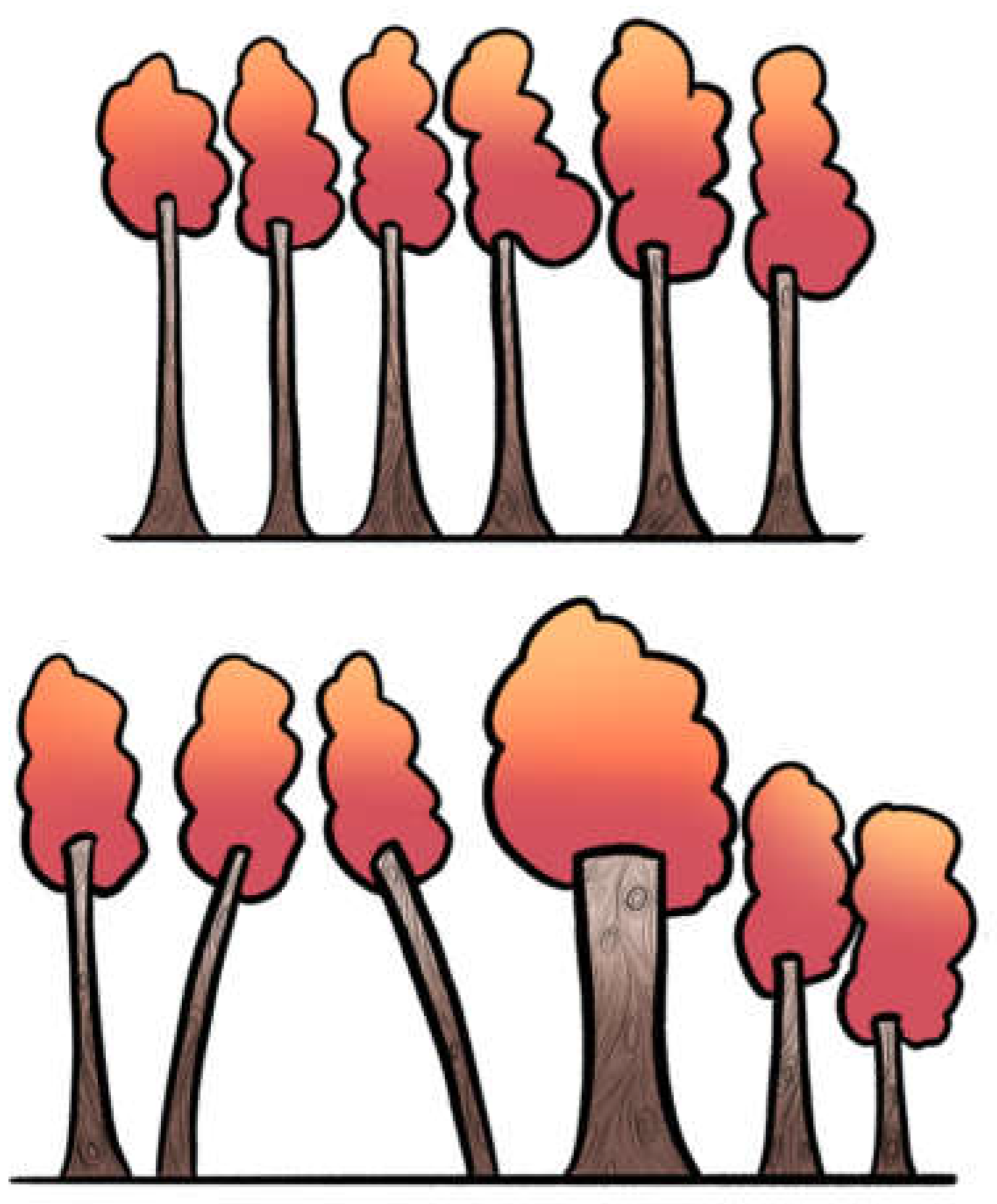
Figure 2.
Different structures of heterogeneity with similar Q. The upper panel depicts several trunks with small variations in height, creating mild irregularity across the skyline. The lower panel shows otherwise symmetric trunks of equal height, except for one that is extremely short. Both scenarios could yield a similar Q statistic, yet they represent very different realities: the same quantification may arise from the progressive accumulation of many small deviations or from a single disproportionate outlier. This underscores that Q reflects the presence of excess variation but does not capture its underlying structure.
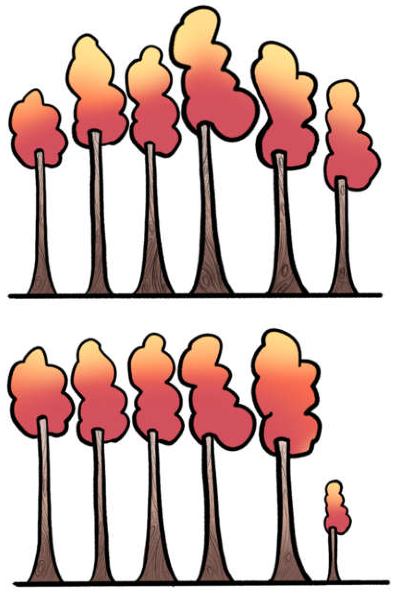
Figure 3.
Same I², different τ². The upper panel shows six trunks: three perfectly vertical and three with a slight tilt. The lower panel mirrors this arrangement, but the tilts are pronounced. Although the proportion of leaning trunks is identical (conceptually the same I²), the degree of tilt differs, representing small versus large τ². This illustrates that I² captures only the proportion of heterogeneity, whereas τ² reflects its magnitude: two meta-analyses may share the same I² yet differ greatly in absolute variability between studies. This illustration is conceptual: in practice, I² depends on Q and study precision, but here the number of leaning trunks is kept constant to show that I² may stay the same while τ² changes.
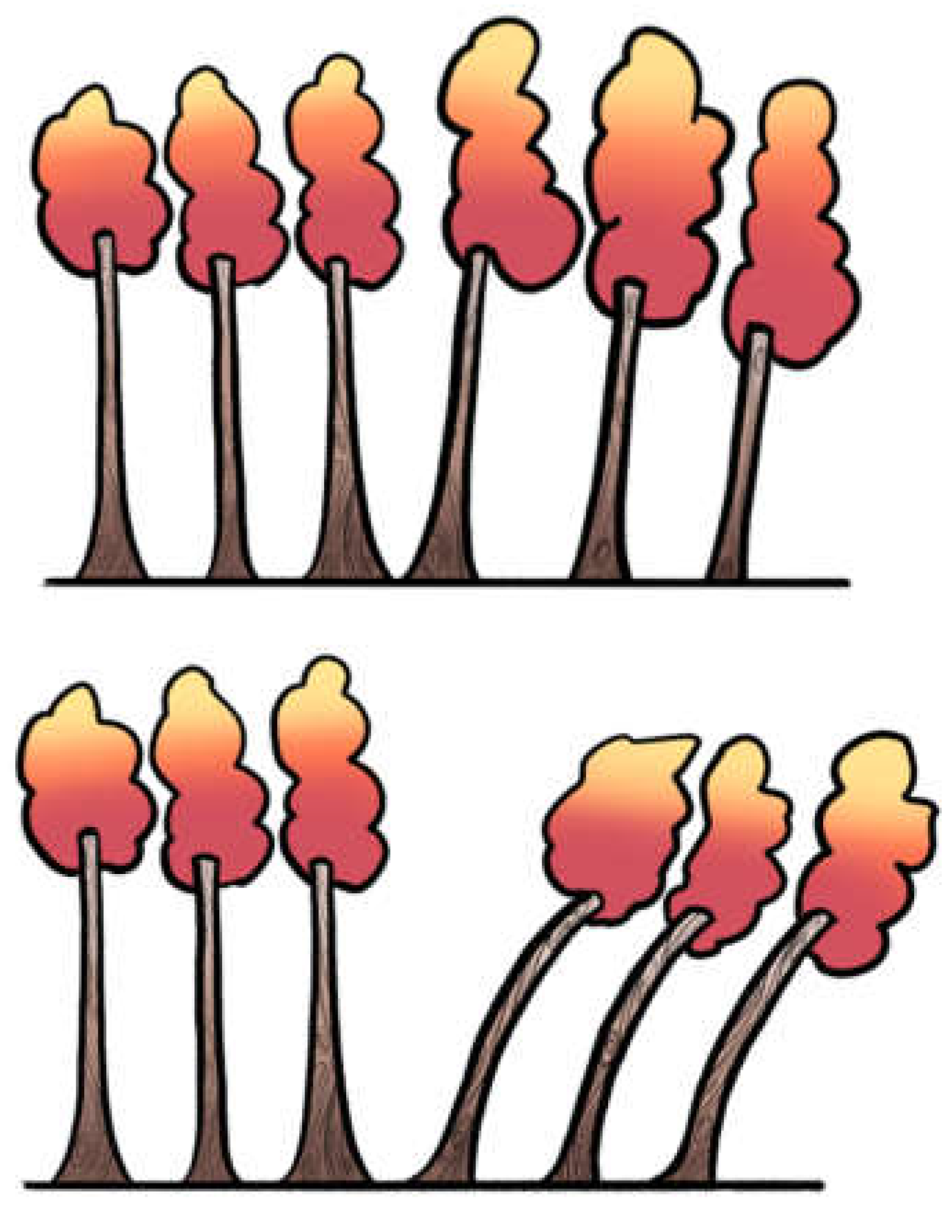

Table 1.
Key statistics for assessing heterogeneity in meta-analysis.
| Measure | What it measures | How it works | Strengths | Limitations | Forest metaphor |
|---|---|---|---|---|---|
| Q (Cochran’s Q) | Tests if variability between studies is greater than chance alone | χ² test, df = n–1 | Simple, widely implemented | Low power with few studies; too sensitive with many; only a test (yes/no) | Spotting whether the grove looks uneven at all |
| I² (Higgins & Thompson) | Proportion of observed variability due to real heterogeneity (not chance) | Derived from Q and df | Intuitive %, widely reported | Distorted with very small/large studies; unstable with few studies; does not tell absolute size | What fraction of the leaning goes beyond natural randomness |
| τ² (tau-squared) | Between-study variance (absolute amount of heterogeneity) | Estimated via formulas (DL, REML, etc.) | Gives scale of dispersion in same units as effect size | Harder to interpret; estimator-dependent; unstable with few studies | How much the trunks lean (a few degrees vs. 40°) |
| Prediction Interval (PI) | Likely range of true effects in a new study | Extends random-effects model using τ² | Adds realism: shows what to expect in future contexts | Wide intervals with few studies; often omitted in practice | Walking deeper: what leaning we may see in the next part of the forest |
| DTA: Univariate Q/I² | Applied separately to sensitivity (Se) and specificity (Sp) | Same formulas as above, but only for one dimension | Easy, familiar | Misleading: ignores correlation Se–Sp, inflates heterogeneity | Looking only east–west, ignoring north–south bends |
| DTA: Bivariate model (Reitsma) | Joint modeling of Se & Sp with correlation (ρ) | Bivariate random-effects linear mixed model on the logit scale of sensitivity and specificity. | Preserves correlation; handles threshold | Requires more data; computationally heavier | Viewing forest in 2D, not one axis |
| DTA: HSROC (Rutter & Gatsonis) | Models accuracy across thresholds | Curve-based hierarchical model | Captures threshold explicitly | Less intuitive for clinicians; complex | Not just leaning trunks, but whole slope of the ground |
| DTA: Bivariate I² (Zhou) | Extends I² to joint Se–Sp space | Formula from bivariate variance-covariance | Provides “intuitive %” in DTA | Newer, less familiar, rarely in software defaults | Proportion of the mess in both directions simultaneously |
Table 2.
Analytical approaches to exploring heterogeneity in meta-analysis.
| Approach | Description | Forest Metaphor | Strengths | Limitations |
|---|---|---|---|---|
| Structured subgroup analysis | Compare effect sizes across categories (e.g. low vs. high RoB, RCT vs. observational). | Comparing clearings: do trees in rocky vs. fertile soil lean differently? | Easy to interpret; highlights clinically meaningful differences. | Strong assumptions; oversimplifies heterogeneity as binary; can be misleading if used alone. |
| Subgroup analysis: Sensitivity analyses | Explore robustness under different assumptions (e.g. estimators, corrections for zero events). | Testing different rulers to measure the same lean. | Reveals how assumptions affect results. | Can be misleading with sparse data; requires multiple studies; exploratory, not confirmatory. |
| Subgroup analysis: leave-one-out | Re-runs meta-analysis omitting one study at a time. | Temporarily removing one tree to see if the skyline changes. | Simple, widely implemented, shows robustness. | Harder to interpret; depends on scale of effect size; unstable with small number of studies. |
| Meta-regression | Relates effect size to study-level covariates (e.g. mean age, year, quality). | Putting on colored lenses—seeing if tilt changes with soil, wind, or slope. | Handles multiple covariates, quantifies trends. | Requires at least 10 studies per covariate |
| Prediction intervals | Estimates range of effect in a future study, considering heterogeneity. | Tells you what tilt angles you might encounter in the next grove. | Clinically meaningful, forward-looking. | Requires a reliable estimate of τ2, which can be difficult when there are only a few studies |
Table 3.
Visual approaches to exploring heterogeneity in meta-analysis.
| Approach | Description | Forest Metaphor | Strengths | Limitations |
|---|---|---|---|---|
| Forest plot visual inspection | Visual inspection of confidence interval overlap across studies. | Looking at tree trunks: do their shadows overlap, or are they scattered apart? | Simple first step; immediately shows obvious dispersion. | Subjective; poor reliability when few studies are available. |
| Baujat plot | Plots each study’s contribution to overall heterogeneity (Q) against influence on effect size. | Spotting which trees lean most and distort the forest skyline. | Identifies outliers and influential studies. | Exploratory; requires enough studies; interpretation not always straightforward. |
| Galbraith (radial) plot | Plots standardized effect sizes against precision. | Like drawing rays from the forest center—outliers stand apart from the main bundle. | Highlights heterogeneity and small-study effects. | Assumes linearity; less intuitive for non-statisticians. |
| L'Abbé plot | Scatterplot of event rates in treatment vs. control groups across studies. | Two groves side by side: do trees from one lean consistently more than the other? | Good for binary outcomes; intuitive clinical insight. | Not suitable for continuous outcomes; harder to interpret with sparse data. |
| Funnel plot | Plots study effect size against precision to assess asymmetry (often for publication bias). | Like looking up at the treetops—symmetry suggests balance, asymmetry suggests something missing. | Can hint at bias or small-study effects; widely recognized. | Low power with few studies; asymmetry ≠ publication bias per se |
Table 4.
Good Practices for Reporting and Interpreting Heterogeneity in Meta-Analysis.
| Step | Recommended Action | Rationale |
|---|---|---|
| 1. Test for Presence | Report Cochran’s Q statistic with degrees of freedom and p-value. | Provides a formal test, but acknowledge its limitations (low power with few studies, excessive sensitivity with many). |
| 2. Quantify Inconsistency | Report I² together with its 95% confidence interval. | I² quantifies the proportion of variability due to heterogeneity. The CI communicates the considerable uncertainty of this estimate. |
| 3. Quantify Magnitude | Report between-study variance (τ²) and specify the estimator used (e.g., REML). | τ² measures the absolute magnitude of heterogeneity. Justify using a robust estimator (REML) over biased methods (DL). |
| 4. Assess Predictive Impact | Report the 95% Prediction Interval. | Translates heterogeneity into a clinically interpretable range of expected effects in future studies. |
| 5. Visualize Data | Always present a forest plot. Consider additional plots (Baujat, Galbraith) if enough studies are available. | Visual inspection complements statistical metrics, helping to identify patterns, outliers, and inconsistencies. |
| 6. Explore Sources with Caution | If subgroup or meta-regression analyses are conducted, explicitly state they are exploratory and hypothesis-generating. | Prevents overinterpretation of findings with low statistical power and high risk of ecological fallacy or spurious results. |
Table 5.
Common Pitfalls (“Don’ts”) in Reporting and Interpreting Heterogeneity.
| Pitfall | Example | Consequence |
|---|---|---|
| Choosing model based on statistical threshold | Switching to random-effects only if Q-test p < 0.10 | Misleading inference; model choice should be conceptually justified, not threshold-driven |
| Using DerSimonian–Laird by default | Applying DL estimator in small or heterogeneous meta-analyses | Underestimation of τ², overly narrow CIs, false precision |
| Overinterpreting subgroup or meta-regression results | Treating subgroup differences as confirmatory | False positives due to low power and ecological bias |
| Ignoring prediction intervals | Reporting only pooled effect and CI | Misses clinical implications of between-study variability |
| Excluding studies based on funnel plot asymmetry alone | Removing “outliers” due to funnel plot | Conflates publication bias with heterogeneity; risks cherry-picking |
| Interpreting or performing funnel plots with few studies (<10) | Drawing conclusions about publication bias from funnel plot when k < 10 | Funnel plots are unreliable with few studies; risk of false inference of bias or asymmetry |
Disclaimer/Publisher’s Note: The statements, opinions and data contained in all publications are solely those of the individual author(s) and contributor(s) and not of MDPI and/or the editor(s). MDPI and/or the editor(s) disclaim responsibility for any injury to people or property resulting from any ideas, methods, instructions or products referred to in the content. |
© 2025 by the authors. Licensee MDPI, Basel, Switzerland. This article is an open access article distributed under the terms and conditions of the Creative Commons Attribution (CC BY) license (http://creativecommons.org/licenses/by/4.0/).
Copyright: This open access article is published under a Creative Commons CC BY 4.0 license, which permit the free download, distribution, and reuse, provided that the author and preprint are cited in any reuse.


