
Submitted:
04 September 2025
Posted:
05 September 2025
You are already at the latest version
Abstract
Background: Accurate evaluation of diagnostic tests is essential to guide clinical decision-making, particularly in surgical practice. Systematic reviews and meta-analyses of diagnostic test accuracy (DTA) are key for evidence synthesis; however, traditional approaches, including univariate pooling or simplified summary ROC (SROC) models such as the Moses–Littenberg method, often yield biased and clinically misleading estimates.Methods: This article presents a methodological guide to hierarchical random-effects models for DTA meta-analysis, structured around current evidence and best practices. Based on this framework, a simulated dataset was generated, and a comprehensive meta-analysis was performed. The analysis illustrates key methodological concepts, interpretation of model outputs, and the use of complementary tools, including likelihood ratios, scattergrams, meta-regression, publication bias assessment, and outlier detection. It also provides a critical comparison of Stata commands for DTA meta-analysis (metandi, midas, metadta), outlining their methodological strengths and limitations to guide researchers in tool selectionResults: The traditional meta-analysis, performed with Meta-DiSc 1.4, applied the DerSimonian–Laird and Moses–Littenberg methods, produced separate sensitivity and specificity pooled estimates with artificially narrow confidence intervals and a symmetric, theoretical SROC curve extrapolated beyond the observed data range, thereby ignoring threshold variability and underestimating between-study heterogeneity. In contrast, the hierarchical random-effects model provided more realistic and clinically interpretable estimates. Joint modeling of sensitivity and specificity revealed substantial between-study variability, a strong negative correlation consistent with a threshold effect, an elliptical confidence region around the summary point (reflecting uncertainty in mean sensitivity/specificity), together with a broader prediction region indicating where 95% of future studies might fall. Influence diagnostics identified outliers and highly influential studies. Conclusions: Promoting the correct application and interpretation of hierarchical models in DTA meta-analyses is essential to ensure high-quality, reliable, and scientifically robust evidence.
Keywords:
Diagnostic accuracy
; Meta-analysis
; Hierarchical models
; HSROC
; Bivariate
; Tutorial
; Stata
Introduction
Accurate diagnostic information is fundamental to surgical decision-making. Surgeons rely on diagnostic tests for key tasks such as patient selection for liver transplantation with non-invasive fibrosis assessment, detection of anastomotic leakage after colorectal surgery using biomarkers, or diagnosis of acute appendicitis with clinical scores. In these contexts, imaging, laboratory tests, and risk scores directly influence indications, timing, and perioperative management.
Systematic reviews and meta-analyses of diagnostic test accuracy (DTA) are crucial for summarizing evidence and shaping clinical practice. However, methodological quality in surgical research remains inconsistent. Many reviews still employ outdated approaches, such as pooling sensitivity and specificity separately using basic random-effects models [1,2], which often yield biased, overly precise, or misleading estimates.
To overcome these limitations, advanced hierarchical models have been developed and are now considered the gold standard. Specifically, the hierarchical summary ROC (HSROC) model proposed by Rutter and Gatsonis [3] and the bivariate random-effects model (BRMA) introduced by Reitsma et al. [4] jointly account for within- and between-study variability, the correlation between sensitivity and specificity, and threshold effects, yielding more reliable estimates.
Despite their advantages and endorsement by the Cochrane Collaboration [5], their application in surgical research is inconsistent, limited by statistical expertise, familiarity, and access to software. As a result, many surgical DTA meta-analyses still produce oversimplified or misleading estimates.
This article provides surgeons and clinical researchers with a practical introduction to hierarchical models for DTA meta-analysis, focusing on their application in surgery. Beyond model structure and interpretation, it highlights complementary tools—such as Fagan nomograms, likelihood ratio scatterplots, and meta-regression—to improve precision and clinical relevance.
Understanding Basic Diagnostic Test Accuracy Metrics: Beyond Sensitivity and Specificity
The diagnostic performance of a test is typically summarized by sensitivity and specificity. Sensitivity is the ability to correctly identify individuals with a disease, while specificity reflects the correct classification of individuals without a disease. Although often presented as intrinsic test properties, both depend on the diagnostic threshold applied [6,7].
In surgical research, thresholds are commonly based on biomarker levels, imaging findings, or clinical scores. For instance, the Alvarado or AIR scores classify the risk of appendicitis using predefined cut-offs, while carcinoembryonic antigen (CEA) thresholds guide surveillance for colorectal cancer recurrence. Lower thresholds increase sensitivity at the expense of specificity, and higher thresholds do the opposite.
A common example is C-reactive protein (CRP), which is used to detect postoperative complications. Studies using lower CRP cut-offs report high sensitivity (≈90%) but low specificity (≈50%), producing false positives. Higher thresholds yield greater specificity (≈85%) but reduced sensitivity (≈65%), increasing false negatives. These trade-offs illustrate the threshold effect, the inverse relationship between sensitivity and specificity across studies [8].
Receiver operating characteristic (ROC) analysis evaluates test performance across all possible thresholds by plotting sensitivity against 1–specificity. The area under the ROC curve (AUC) summarizes overall discrimination: 1 indicates perfect accuracy, 0.5 random chance [9,10,11]. Although widely reported, AUC is threshold-independent and does not reflect performance at clinically relevant cut-offs. Reporting sensitivity, specificity, and likelihood ratios at defined thresholds, therefore, remains essential.
Positive and negative predictive values (PPV, NPV) describe the probability of disease given a positive or negative test [12]. However, both depend strongly on disease prevalence: in low-risk populations, PPV is low, while in high-risk groups, PPV increases.
Likelihood ratios (LRs) provide prevalence-independent measures [13,14]. LR+ quantifies how much more likely a positive result is in diseased versus non-diseased individuals; LR– expresses how much less likely a negative result is in diseased versus non-diseased individuals. In practice, an LR+ >10 supports disease confirmation, while an LR– <0.1 supports exclusion. However, such extreme values are rare in surgical research, where most tests yield intermediate ratios that only modestly shift diagnostic probability. For instance, pooled analyses of the Alvarado score in children show an LR+ ≈2.4 and an LR– ≈0.28: useful for refining suspicion but insufficient to rule in or rule out appendicitis [15].
The Diagnostic Odds Ratio: Interpretation and Limitations
The diagnostic odds ratio (DOR) is frequently reported in systematic reviews and meta-analyses as a global indicator of test performance. It expresses how much greater the odds of a positive test are in diseased individuals compared with non-diseased. Here, “odds” means the probability of an event divided by the probability of it not occurring (p / [1–p]). For example, if a test detects disease in 80% of cases, the odds are 0.8 / 0.2 = 4. Mathematically, the DOR is calculated as:
DOR = (TP × TN) / (FP × FN)
Higher DOR values indicate better discrimination, with 1 reflecting no diagnostic ability [16]. However, the DOR has significant limitations: it compresses sensitivity and specificity into a single number, hides clinically relevant trade-offs, and lacks intuitive interpretation.
This limitation is particularly relevant in surgical contexts, where priorities differ. Maximizing sensitivity is crucial for diagnosing postoperative complications, such as anastomotic leakage, where false negatives can be particularly dangerous. Conversely, maximizing specificity is essential when considering reoperation for suspected bile duct injury, where false positives may lead to unnecessary surgery. The DOR, as a single global estimate, cannot capture these context-specific trade-offs or threshold effects.
The DOR lacks intuitive clinical interpretation. Unlike sensitivity, specificity, or LRs, it does not translate into probabilities and may overestimate a test’s value.
It is essential to distinguish the DOR from the conventional odds ratio (OR). Although mathematically similar, the OR measures exposure–outcome association, not diagnostic performance. As Pepe et al. note, a significant OR does not imply clinically useful accuracy [17].
Thus, while the DOR may be reported for completeness, it should not be the primary indicator of diagnostic performance. Sensitivity, specificity, likelihood ratios, and post-test probabilities remain the essential, clinically interpretable metrics.
Why Hierarchical Models Are Needed in Diagnostic Test Accuracy Meta-Analyses
Diagnostic research is inherently heterogeneous. Populations differ in demographics and disease prevalence, reference standards are inconsistent, and diagnostic tools vary in technique and operator expertise. For example, appendicitis scores show different accuracy in children versus adults; radiological criteria for bile duct injury after cholecystectomy are not uniform; and biomarker assays such as CRP or procalcitonin vary depending on whether ELISA, high-sensitivity, or point-of-care methods are used. Study design (prospective vs. retrospective), risk of bias, and post hoc threshold adjustments add further variability.
A central source of heterogeneity is the threshold effect: adjusting the positivity cut-off directly shifts the balance between sensitivity and specificity. For instance, lowering a CRP cut-off after colorectal surgery raises sensitivity (fewer missed leaks) but lowers specificity (more false positives). Raising the threshold has the opposite effect.
Conventional pooling methods—such as DerSimonian–Laird or the Moses–Littenberg SROC [18]—ignore this correlation by imposing a fixed symmetric ROC relationship that cannot capture threshold-specific effects. As a result, they often underestimate heterogeneity and give overly precise, clinically misleading estimates. Despite these limitations, they are still used, mainly due to reliance on outdated tools like Meta-DiSc 1.4 or RevMan.
Hierarchical models address these shortcomings. The HSROC model [3] and the bivariate model [4] jointly synthesize sensitivity and specificity, incorporate threshold effects, and model both within- and between-study heterogeneity. Their outputs include summary points, HSROC curves, and variance components that reflect real-world variability. For these reasons, hierarchical models are endorsed by methodological authorities, including the Cochrane Handbook, as the gold standard for DTA meta-analysis [19,20].
Hierarchical Models for DTA Meta-Analyses: Structure and Parameterization
The term ‘hierarchical’ means that the model operates on two levels at once: it accounts for uncertainty within each individual study and simultaneously models the variability between studies.
Two hierarchical random-effects models are considered the methodological standard: the HSROC model [3] and the bivariate random-effects model (BRMA) [4]. Both share the same statistical foundation, allowing joint synthesis of sensitivity and specificity while modeling their correlation and between-study heterogeneity.
The HSROC model assumes each study reflects an underlying ROC curve, with threshold variability contributing to heterogeneity. Its parameterization—Λ (accuracy), Θ (threshold), β (slope), σ²ₐ (variance for accuracy), and σ²ₜₕ (variance for threshold)—produces a global ROC curve with confidence regions. It is particularly useful when studies apply different thresholds, as the summary curve is more informative than a single pooled point.
The BRMA model directly analyzes logit-sensitivity and logit-specificity, preserving their correlation. The logit is a mathematical transformation that converts proportions such as sensitivity and specificity (bounded between 0 and 1) into values on the entire real line, stabilizing variances and making the data more suitable for linear modeling. Parameters include μₐ (mean logit-sensitivity), μᵦ (mean logit-specificity), σ²ₐ (variance for sensitivity), σ²ᵦ (variance for specificity), and ρₐᵦ (the correlation between logit-sensitivity and logit-specificity). This parameterization produces a summary point estimate with confidence and prediction regions, which is especially meaningful when studies use the same threshold, providing a concise pooled estimate.
Both HSROC and BRMA models are statistically robust and produce equal results under most conditions, particularly in the absence of covariates or meta-regression. Their use is endorsed by leading methodological authorities, including the Cochrane Handbook for DTA Reviews [5], as essential tools for generating valid, reliable, and clinically interpretable estimates of diagnostic accuracy. However, confusion in terminology persists, as the terms “bivariate model,” “hierarchical model,” and “HSROC” are often used interchangeably. While both derive from the same framework, they differ in parameterization and interpretative focus. Selecting the appropriate model depends on whether studies use common thresholds (favoring BRMA) or varying thresholds (favoring HSROC).
Which Metrics Should Be Reported in Diagnostic Test Accuracy Meta-Analyses
DTA meta-analyses should report clinically interpretable and statistically robust parameters. Core metrics include pooled sensitivity and specificity with 95% CIs, LR+ and LR– with CIs, and the HSROC curve and summary point with its confidence and prediction regions [5].
As previously discussed, both AUC and DOR have important limitations; they may be included for completeness but should never replace sensitivity, specificity, or likelihood ratios as primary measures.
Finally, confidence intervals depend on the method used. Exact approaches such as Clopper–Pearson yield wider, more conservative bounds that better reflect uncertainty, especially with small samples or extreme proportions. Modern implementations in R and Stata rely on more advanced and robust methods that incorporate between-study heterogeneity more appropriately.
Selecting the Appropriate Statistical Software for Diagnostic Accuracy Meta-Analysis
The correct application of hierarchical models depends not only on conceptual understanding but also on appropriate software. Although HSROC and BRMA are considered the gold standard, many commonly used platforms either lack support for these models or present substantial limitations [21].
Several options exist, including Meta-DiSc [22], RevMan [23], R [24], SAS [25], and Stata [26]. Meta-DiSc v1.4 does not implement hierarchical models, instead relying on separate pooling with the DerSimonian–Laird method or simplified SROC curves based on the Moses–Littenberg method. These approaches partly account for sensitivity–specificity correlation but cannot model threshold variability or heterogeneity, often producing biased or overly optimistic estimates. The more recent Meta-DiSc 2.0 incorporates hierarchical modeling, although its functionality remains limited compared to R or Stata. RevMan (v5.4) is also widely used but restricted to traditional, non-hierarchical methods.
By contrast, R and Stata allow the correct application of hierarchical models. R, as an open-source environment, provides extensive functionality (BRMA, HSROC, meta-regression, advanced visualizations) but requires programming skills. SAS [25] also supports hierarchical modeling but is less accessible due to licensing and limited adoption in surgical research.
Stata (StataCorp LLC, College Station, TX) [26] provides a balanced alternative, combining extensive analytical capabilities with greater user accessibility. Within Stata, three commands—metandi (Harbord & Whiting), midas (Dwamena), and metadta (Nyaga & Arbyn) [27,28,29,30]—enable hierarchical DTA workflows with important differences. Both metandi and metadta fit the BRMA and derive HSROC parameters/curves by formal re-parameterization; they do not fit a second HSROC model. midas draws a ROC curve as a continuous extrapolation of BRMA output, not a formally parameterized HSROC; consequently its AUC and prediction region are approximations.
- metandi [27]: Was the first Stata command for hierarchical DTA meta-analysis. It is more limited in scope but provides a detailed output of all core model parameters. However, it lacks meta-regression and offers only limited graphical customization.
- midas [28]: Although limited in some aspects, it remains a complementary option for hierarchical modeling. It integrates exploratory tools, including heterogeneity plots, goodness-of-fit checks, Fagan nomograms, likelihood ratio scattergrams, and Deeks’ regression test for publication bias. It can estimate the AUC with 95% CI, but these values may be biased since they are not obtained from a formal HSROC model. Meta-regression is available but restricted to univariable analyses (although multiple univariates can be displayed simultaneously on screen, as illustrated in this article). A practical caveat is that midas may occasionally return an AUC of 1.0 with CI 0–1 if the Excel file contains hidden rows; deleting unused rows or copying data into a new clean sheet resolves this issue.
- metadta [29,30]: Is the most modern and versatile Stata command for DTA meta-analysis. It offers extensive functionalities, including bivariate I² estimation (Zhou et al.), advanced meta-regression capabilities, and highly customizable graphical outputs. It is currently the preferred tool for conducting methodologically rigorous DTA meta-analyses within the Stata environment. Nonetheless, it has some limitations in specific analyses, particularly regarding graphical utilities, where midas provides complementary features (e.g., Fagan nomograms, likelihood ratio scattergrams, and integrated diagnostic plots).
Table 1 presents the main distinctions among the Stata commands most commonly used to implement these models (metandi, midas, and metadta).
In summary, while multiple software options exist for DTA meta-analysis, only a subset enables appropriate hierarchical modeling aligned with current methodological standards. Stata provides a robust, accessible environment, with metadta [29,30] representing the most comprehensive option for producing clinically meaningful and statistically sound syntheses of diagnostic performance. Equivalent hierarchical workflows are available in R (e.g., mada, diagmeta) for open-source implementations.
Heterogeneity in Diagnostic Test Accuracy Meta-Analyses
Heterogeneity is one of the most significant challenges in meta-analysis of diagnostic test accuracy (DTA). It can arise from multiple sources, including differences in patient populations, disease prevalence, reference standards, study design, and methodological quality. Threshold selection is also a key contributor: lowering a cut-off usually increases sensitivity at the expense of specificity, while raising it has the opposite effect.
Traditional measures of heterogeneity widely used in intervention reviews, such as Cochran’s Q test and Higgins’ I² statistic [31], are not appropriate in this context. They ignore the intrinsic correlation between sensitivity and specificity caused by threshold effects and can therefore overestimate or misrepresent between-study variability.
To address this, Zhou et al. proposed a bivariate I² [32], which jointly accounts for variability and correlation within the hierarchical framework. When reported together with τ² estimates for sensitivity and specificity, and complemented by prediction regions in HSROC or BRMA plots, it provides a more accurate and clinically meaningful picture of residual heterogeneity. The bivariate I² has been implemented in metadta [29,30] and is increasingly considered a complementary valid tool for quantifying heterogeneity in DTA meta-analyses.
As a preliminary exploratory step, many DTA meta-analyses report the Spearman correlation coefficient (ρ), which evaluates the relationship between sensitivity and specificity across studies. A strong negative correlation suggests the presence of threshold effects, where differences in positivity thresholds drive the sensitivity–specificity trade-off [5].
Beyond global heterogeneity estimates, BRMA provides variance components for sensitivity (σ²ₐ) and specificity (σ²ᵦ), which quantify between-study variability not explained by within-study precision. Larger values indicate greater heterogeneity and reduced reproducibility of diagnostic performance.
While informative, Spearman’s ρ is only a unidimensional approximation and cannot capture the multidimensional heterogeneity addressed by hierarchical models. It is important to stress that a high absolute ρ should not be interpreted as a literal percentage of heterogeneity explained, nor as interchangeable with the model-based correlation (ρₐᵦ). For clarity, the reported correlation must always be specified explicitly. Properly framed, the two serve distinct purposes: Spearman’s ρ is exploratory, generating hypotheses about threshold effects, whereas ρₐᵦ is the formal inferential parameter within BRMA, as it accounts for study precision.
Finally, prediction regions from BRMA offer a graphical representation of heterogeneity. These regions define the expected range in which 95% of future studies are likely to fall, complementing confidence intervals and providing an intuitive visualization of between-study variability.
Meta-Regression in Diagnostic Test Accuracy Meta-Analyses
Beyond global summary estimates, exploring sources of heterogeneity is essential to improve the clinical interpretability and methodological rigor of DTA meta-analyses [5]. A critical methodological requirement is that potential covariates for meta-regression be defined a priori; post hoc selection constitutes data dredging and inflates the risk of spurious associations.
Meta-regression extends hierarchical models by evaluating whether study-level covariates—such as study design (prospective vs. retrospective), patient population (pediatric vs. adult), risk of bias (QUADAS-2), disease prevalence, or diagnostic thresholds—explain variability in sensitivity, specificity, or overall performance. Univariable analyses examine covariates individually, while multivariable approaches allow simultaneous adjustment for several factors. Although more informative, the latter requires larger datasets; methodological guidance recommends at least 10 studies per covariate to reduce type I error and instability [5].
Even when pre-specified, meta-regression remains exploratory and observational. Associations must not be interpreted as causal, as they may reflect residual confounding, ecological bias, or imbalanced covariate distributions. Limited power is common in DTA research, further amplifying the risk of misleading or unstable results.
Applied with caution, meta-regression can nevertheless yield valuable insights into how diagnostic performance varies across settings, populations, and methodological designs, refining evidence synthesis and guiding future research priorities.
Publication Bias in Diagnostic Test Accuracy Meta-Analyses
Publication bias is a recognized threat to the validity of meta-analyses, including those of DTA. It occurs when studies with favorable diagnostic performance—such as high sensitivity, specificity, or DOR—are more likely to be published, inflating pooled estimates and generating misleading conclusions.
Detecting publication bias in DTA poses methodological challenges. Classical tools—funnel plots, Begg’s test, and Egger’s regression—are widely used in intervention research, but they assume a single continuous effect size and independence between outcomes. These assumptions do not hold in DTA because sensitivity and specificity are paired [33,34]. Consequently, applying Begg’s or Egger’s tests is inappropriate in DTA and may produce misleading results [5,35,36].
To address this, Deeks’ regression test was specifically developed for DTA. It regresses the log DOR against the inverse square root of the effective sample size; smaller studies with exaggerated performance estimates cluster asymmetrically. A significant slope (p < 0.1) suggests small-study effects, potentially indicating publication bias. The Cochrane Handbook and other major guidelines endorse Deeks’ test. However, it has limited power when <10 studies are available, so results must be interpreted cautiously. Also, even with more studies, its power is often modest, and a non-significant Deeks test does not exclude publication bias; it indicates insufficient evidence for small-study effects given the available data.
In Stata, midas incorporates a subcommand (pubbias) that implements Deeks’ test and produces a graphical output. In contrast, metandi and metadta do not include this function, requiring complementary tools (e.g., midas or manual coding).
Publication bias is only one of several possible biases in DTA meta-analysis. Others include spectrum bias, selection bias, partial verification bias, misclassification, information bias, and disease progression bias. Most tend to overestimate accuracy, though in some contexts they may underestimate it [2]. Considering these factors alongside formal publication bias assessment is critical for a transparent and clinically meaningful synthesis.
Complementary Tools for Interpreting DTA Meta-Analyses: Fagan Nomograms, Scatterplots, and Beyond
Beyond summary estimates and HSROC curves, complementary tools improve the clinical interpretability of DTA meta-analyses, bridging statistical outputs with practical decision-making in surgery and other high-stakes settings.
The Fagan (Bayesian) nomogram is widely used to translate test accuracy into clinically relevant terms [37]. It illustrates how pre-test probability, likelihood ratios (LR+ and LR−), and post-test probability interact. By applying likelihood ratios from a meta-analysis to an estimated pre-test probability, clinicians can approximate post-test probabilities, facilitating risk stratification and diagnostic reasoning.
Likelihood ratio scatterplots provide another intuitive display [38]. Unlike ROC scatterplots, they plot LR+ against LR− across studies, highlighting variability, outliers, or subgroup effects. The scattergram defines four quadrants of informativeness:
- Upper Left Quadrant: LR+ < 10, LR− < 0.1 — diagnostic exclusion only
- Upper Right Quadrant: LR+ > 10, LR− < 0.1 — both exclusion and confirmation
- Lower Right Quadrant: LR+ > 10, LR− > 0.1 — diagnostic confirmation only
- Lower Left Quadrant: LR+ < 10, LR− > 0.1 — neither exclusion nor confirmation
This allows rapid assessment of a test’s confirmatory and exclusionary potential, complementing AUC or DOR.
Model diagnostics further evaluate heterogeneity and influence. Cook’s distance quantifies the leverage of each study: a study is influential if its value is much larger than others [27]. Standardized residuals indicate misfit, with values beyond ±2 suggesting outliers. Used together, they reveal whether specific studies disproportionately alter sensitivity, specificity, or thresholds.
In midas [28], these analyses are integrated into a simplified workflow suitable for clinicians or researchers without advanced statistical expertise. The modchk command generates four diagnostic plots: (1) residuals for goodness-of-fit, (2) a probability plot for bivariate normality, (3) Cook’s distance for influential studies, and (4) standardized residuals to evaluate model fit at the study level. While practical, midas does not implement a formally parameterized HSROC model. Consequently, its outputs may differ from those produced by more rigorous tools such as metandi [27] or metadta [29,30].
Prediction regions in midas HSROC plots are often exaggerated because the program sums the variances of logit-sensitivity and logit-specificity without accounting for their negative covariance, markedly inflating the region [28]. By contrast, metadta [29,30] incorporates Zhou’s bivariate I² [32], providing a more accurate and robust representation of heterogeneity and prediction intervals.
Bivariate boxplots, also available in midas [28], offer another way to explore heterogeneity by plotting logit-sensitivity against logit-specificity. Concentric regions represent the expected distribution under a bivariate normal model, and studies outside the outer envelope are flagged as potential outliers. Such studies often display atypical sensitivity–specificity trade-offs due to threshold effects, distinct populations, or methodological variability. In the analysis, the bivariate boxplot identified four outliers, including studies with unusually high sensitivity but low specificity, and others with distorted trade-offs linked to elevated thresholds or pediatric cohorts. When interpreted alongside Cook’s distance and standardized residuals, this tool provides a robust visual assessment of data integrity and sources of heterogeneity beyond numerical summaries.
Together, these complementary tools—when appropriately applied—enhance the transparency, diagnostic validity, and clinical utility of DTA meta-analyses, supporting reliable evidence synthesis for decision-making.
Table 2 summarizes the main differences between classical and hierarchical models in their application to DTA reviews.
Application of Hierarchical Models in Surgical Diagnostic Research: A Practical Example
To illustrate the practical implications of model selection in DTA meta-analyses, a simulated dataset of 30 studies was generated to evaluate a hypothetical biomarker for diagnosing a surgical condition. The dataset was designed to reflect common features of real-world surgical research, including threshold variability, between-study heterogeneity, and a marked threshold effect.
Let’s suppose that, as part of the meta-analytic design, the analytical strategy was pre-specified a priori (as it should be), with covariates, models, and sensitivity analyses defined before looking at the results. Three covariates were pre-specified as clinically and methodologically relevant for subsequent meta-regression: (i) risk of bias in the index test domain of QUADAS-2, due to the continuous nature of the biomarker and the risk of overfitting when thresholds are defined post hoc; (ii) study population (adult vs. pediatric), reflecting inherent differences in diagnostic performance; and (iii) study design (retrospective vs. prospective), given its potential to introduce bias. This pre-hoc specification ensured that the analyses followed a transparent, hypothesis-driven framework rather than exploratory data dredging. For illustrative purposes, all covariates in this example were treated as dichotomous variables to simplify the demonstration of syntax and interpretation. However, it is essential to stress that dichotomization of continuous covariates is methodologically discouraged in real analyses, as it reduces power and may create artificial associations. Importantly, although multiple covariates were explored here, formal meta-analyses should avoid testing numerous regressions without adequate power. Best practice is to pre-specify in the protocol a limited set of one or two clinically justified covariates, ensuring at least 10 studies per covariate to support valid inference.
Subsequently, a properly structured dataset was assembled in spreadsheet format (e.g., Excel). It included a study identifier (commonly labeled as studyid; study_id; or id), followed by 2×2 contingency data: true positives (tp), false positives (fp), false negatives (fn), and true negatives (tn), ideally in that order. In real-world datasets, if a study contained a zero cell in its 2×2 table, continuity correction (e.g., adding 0.5 to all four cells) or Bayesian models were applied to enable logit transformations. Some statistical packages/commands (e.g., metandi) failed when zero cells were present. In contrast, more modern implementations, such as metadta, handled them automatically (e.g., by fitting the model directly on the binomial likelihood rather than on logit-transformed proportions).
Additional columns incorporated the three pre-specified study-level covariates. In meta-regression, dichotomous covariates are coded in a binary fashion: the reference category is coded as 0 (“No”), and the comparison category as 1 (“Yes”). Accordingly, high risk of bias in the index test domain of QUADAS-2 (No vs. Yes), pediatric population (No vs. Yes), and study design (retrospective vs. prospective) were coded following this convention. This dataset exemplified the recommended structure before initiating a DTA meta-analysis. It is important to note that this framework assumed a single threshold per study. When individual studies reported multiple thresholds, one had to be selected, or specialized methods—such as bivariate ROC curve meta-analysis—were applied, which are beyond the scope of this guide.
The Conventional (Flawed) Analysis: Meta-DiSc
Initially, a conventional, non-bivariate meta-analysis was applied using Meta-DiSc (version 1.4). Separate random-effects models (DerSimonian-Laird) were used to pool sensitivity and specificity independently, and a symmetric SROC curve was generated using the Moses-Littenberg method. As expected, this approach ignored threshold variability, between-study heterogeneity, and the intrinsic correlation between sensitivity and specificity. The results appeared falsely precise, with narrow confidence intervals: pooled sensitivity, 0.74 (95% CI: 0.73–0.76); specificity, 0.68 (95% CI: 0.66–0.69); and heterogeneity exceeding 94% (I²) for both. The area under the SROC curve (AUC) was 0.7881; however, no confidence intervals were provided, which limits interpretability (Figure 1).
The Hierarchical Analysis: A Robust Alternative with Stata
In contrast, re-analysis using hierarchical models in Stata Statistical Software, Release 19 (StataCorp LLC, College Station, TX) (metandi, midas, metadta) implemented the BRMA framework, accounting for threshold effects, heterogeneity, and the correlation between sensitivity and specificity. All three approaches generated both pooled summary points and HSROC curves. The estimated AUC, as estimated by midas through extrapolation of the bivariate model parameters across the full 0–1 specificity range, was 0.79 (95% CI: 0.75–0.82), with summary sensitivity 0.74 (95% CI: 0.66–0.81) and specificity 0.71 (95% CI: 0.63–0.79). LR+ was 2.6 (95% CI: 2.1–3.2), and LR- was 0.36 (95% CI: 0.3–0.44). The DOR was 7 (95% CI: 6-9). Wider confidence intervals accurately reflected underlying uncertainty. Between-study variance (τ²) remained substantial: 0.99 for sensitivity, 1.14 for specificity. A strong negative correlation (ρₐᵦ = –0.87) confirmed a pronounced threshold effect—completely overlooked by the non-hierarchical model (Figure 2). τ² for sensitivity and specificity, together with ρₐᵦ, were explicitly estimated using both metandi and metadta in Stata. In addition, the bivariate I² implemented in metadta showed substantial inconsistency overall (I² = 85.1%), which—although still high—was notably lower than the univariate I² values for sensitivity (91.5%) and specificity (92.6%) obtained in the same model, indicating that the generalized metric provides a more balanced quantification of residual heterogeneity.
Visual inspection of the HSROC plots revealed that the prediction regions produced by metandi and metadta were of moderate size, consistent with residual heterogeneity. In contrast, midas generated a methodologically incorrect prediction region. This occurs because midas sums the between-study variances of logit-sensitivity and logit-specificity as if they were independent, ignoring their strong negative covariance. Such an univariate approximation inflates the total variance and prediction region, producing a statistically invalid and potentially misleading representation of heterogeneity. Conversely, metadta implements the bivariate I² of Zhou et al., providing a more accurate, correlation-adjusted estimate of heterogeneity and prediction intervals.
Although the global AUC values appear similar (0.79 vs. 0.788), the comparison is misleading: the conventional SROC AUC was reported without confidence intervals, reflecting its speculative nature and tendency to overestimate accuracy, whereas the hierarchical AUC (0.79, 95% CI: 0.75–0.82) is statistically grounded. Thus, the apparent agreement in point estimates should not be overinterpreted, as only the hierarchical model provides a reliable measure with quantified uncertainty. It should also be noted that AUCs from midas represent an inferential extrapolation across the full 0–1 specificity range, which can be optimistic compared with formally parameterized HSROC estimates.
Investigating Heterogeneity: Influence Diagnostics and Outlier Detection
Initial heterogeneity exploration included influence diagnostics using Cook's distance and standardized residuals derived from metandi. This dual approach quantified the influence of individual studies and their deviation from model expectations. Most studies aligned well with the predicted values; however, Study 5 exhibited high influence, with a Cook’s distance markedly greater than that of all other studies (Supplementary File 2, top panel). At the same time, its standardized residual for sensitivity was moderate, at approximately –1. Other studies showed more extreme standardized residuals (Supplementary File 2, middle panel) yet had less overall influence, underscoring that influence was a composite measure of both a study’s leverage and its deviation from the model’s prediction (Supplementary File 2, middle panel).
To assess the impact of influential Study 5, the hierarchical meta-analysis was repeated, excluding it. Summary point estimates for sensitivity and specificity changed only modestly (sensitivity: 0.75 [95% CI 0.67–0.81]; specificity: 0.71 [95% CI 0.62–0.79]), and between-study variance components remained essentially unchanged (τ² for sensitivity: 0.99 → 0.96; τ² for specificity: 1.14 → 1.18). This showed that although Study 5 exerted disproportionate influence on model fit (high Cook’s distance), it did not materially alter the overall heterogeneity structure. Its role was therefore better understood as an influential point in terms of leverage rather than as the dominant driver of between-study variability, with the strong negative correlation between sensitivity and specificity (ρₐᵦ = –0.96) confirming a persistent threshold effect.
To complement these analyses, a bivariate boxplot of logit-transformed sensitivity and specificity was generated (Supplementary File 2, bottom panel). Four studies fell outside the expected envelope—Studies 1, 11, 12, and 21—indicating atypical patterns that may reflect diagnostic trade-offs, threshold variability, or population-specific effects.
Although the summary point changed modestly (Se 0.74→0.69; Sp 0.71→0.74), the material finding is a ~35% reduction in τ² for sensitivity (0.99→0.64), showing that a few atypical studies were the main source of between-study variability in sensitivity. Thus, while the pooled estimates appear robust, the reproducibility and generalizability of sensitivity across settings remain less stable, as they depend heavily on a small number of outliers. The strong negative correlation between sensitivity and specificity (ρₐᵦ = –0.76) persisted, consistent with a threshold effect.
Exploring Sources of Heterogeneity: Meta-Regression
After that, univariable meta-regressions in midas were used to evaluate the predefined covariates. The most consistent signal arose from study quality: high-risk studies—typically characterized by retrospective or post hoc threshold selection—showed inflated diagnostic accuracy (sensitivity 0.79; specificity 0.80) relative to low-risk studies (sensitivity 0.72; specificity 0.67), a pattern consistent with overfitting. Neither study design nor population type materially altered diagnostic performance (Supplementary File 3).
Translating Results into Clinical Practice: Fagan Nomograms and Likelihood Ratios
Lastly, Fagan nomograms translated these findings into clinical terms for two scenarios: low pre-test probability (10%, e.g., general screening) and high pre-test probability (50%, e.g., symptomatic surgical patients) (Supplementary File 4). With LR+ ≈ 3 and LR− ≈ 0.36, the test modestly altered diagnostic probability: in low prevalence settings, a positive result increased post-test probability to 22%, while a negative result reduced it to 4%; in high-risk patients (50% pre-test probability), a positive result increased post-test probability to 72%, while a negative result reduced it to 27%. While this shift in probabilities may inform clinical suspicion, it is often insufficient to definitively rule in or rule out the condition, leaving many patients in an intermediate-risk category that typically requires further testing.
The LR scattergram further summarized diagnostic performance, with pooled LR+ ≈ 3 and LR− ≈ 0.3, positioned in the lower right quadrant—indicating limited confirmatory and exclusionary value. The wide distribution of individual studies reinforced the presence of substantial heterogeneity (Supplementary File 5).
Assessing Publication Bias: Deeks' Test
To assess publication bias, Deeks’ test was applied via midas. The regression analysis revealed no significant small-study effect (P = 0.6), and the plot showed no visual asymmetry, indicating a low risk of publication bias (Supplementary File 6).
This example illustrates that outdated approaches, such as the Moses-Littenberg method, overlook crucial methodological factors, leading to misleading precision. In contrast, when applied properly, hierarchical models and complementary tools yield robust and clinically meaningful insights into diagnostic performance. Also, as this practical example demonstrates, a comprehensive and robust DTA meta-analysis in Stata currently requires a combined workflow, leveraging the unique strengths of several commands, as no single tool provides a complete solution.
Supplementary File 7 includes the Stata code used for the statistical analyses.
Common Pitfalls, Expertise Requirements, and Practical Recommendations
Despite the clear advantages of hierarchical and bivariate models, their correct use in DTA meta-analyses requires both statistical expertise and clinical judgment. Methodological errors continue to undermine the validity of published reviews.
A common pitfall is reliance on outdated methods, such as univariate pooling of sensitivity and specificity, which ignore their correlation and threshold effects. Similarly, platforms without hierarchical modeling (e.g., Meta-DiSc, RevMan) often yield artificially narrow confidence intervals, underestimated heterogeneity, and inflated performance estimates.
Even when hierarchical models are applied, misinterpretation remains frequent. Errors include misunderstanding heterogeneity metrics (e.g., τ², I²), overemphasizing global indicators like AUC or DOR, or neglecting threshold variability. Reporting AUC without clarifying its derivation, or treating DOR as the main outcome, oversimplifies results and obscures clinically relevant nuances.
To ensure robust, clinically meaningful evidence synthesis, several recommendations should be followed:
- Select appropriate, validated software for hierarchical modeling, prioritizing tools such as metandi, midas, or metadta in Stata, or equivalent R packages (mada, diagmeta), depending on available expertise and project complexity.
- Report comprehensive diagnostic metrics, including pooled sensitivity and specificity with confidence intervals, HSROC curves, and likelihood ratios. The DOR may be included as a secondary indicator, but should not be the sole measure of test performance. If reporting the AUC, clarify whether it derives from a rigorously parameterized HSROC model or a simplified approximation, as interpretations differ substantially.
- Use prediction intervals and heterogeneity estimates, such as τ² or the bivariate I² by Zhou, to convey uncertainty and between-study variability transparently. Avoid overreliance on conventional I², which exaggerates heterogeneity by ignoring the correlation between sensitivity and specificity.
- Incorporate complementary graphical and analytical tools, including Fagan nomograms, likelihood ratio scatterplots, Cook’s distance, and standardized residuals, to enhance interpretability, identify influential studies, and explore sources of heterogeneity. It is essential to distinguish between post hoc sensitivity analyses and post hoc meta-regression. The former are an accepted strategy to test the robustness of primary findings when influential or outlying studies are identified. Their role is to confirm whether conclusions hold when such studies are excluded, not to produce a ‘new correct’ result. In contrast, deciding covariates for meta-regression post hoc constitutes data dredging and increases the risk of spurious associations. Robust practice requires pre-specifying covariates a priori in the protocol, whereas outlier-based sensitivity analyses should be presented transparently as exploratory robustness checks. Even when pre-specified, meta-regression findings must be interpreted with caution, particularly in small meta-analyses, where introducing multiple covariates risks overfitting. A commonly recommended rule of thumb is to ensure at least 10 studies per covariate to achieve stable inference.
- Recognize and mitigate additional biases beyond publication bias, such as spectrum bias (non-representative patient populations), selection bias, partial verification bias, misclassification, information bias, or disease progression bias. These sources of error frequently lead to overestimation of diagnostic performance, underscoring the need for rigorous methodological safeguards.
- Collaborate with experienced biostatisticians or methodologists throughout all phases of the meta-analysis, from dataset preparation to statistical modeling and interpretation, to ensure adherence to best practices and maximize methodological rigor.
- Explicitly verify the statistical assumptions underpinning hierarchical models. Many users apply BRMA or HSROC frameworks without assessing residual distribution, bivariate normality, or the influence of individual studies. Tools such as midas modchk or the influence diagnostics in metandi facilitate this evaluation and should be part of routine analysis. If bivariate normality is seriously violated (e.g., highly skewed distributions), consider data transformations, alternative modeling strategies such as more flexible Bayesian approaches, or, at the very least, interpret the results with great caution.
- Interpret results with caution in small meta-analyses. When fewer than 10 studies are included, hierarchical models remain the preferred approach, but confidence intervals widen, prediction regions expand, and estimates of heterogeneity or threshold effects become less stable. In such scenarios, emphasis should shift towards transparency, identification of evidence gaps, and cautious interpretation rather than overconfident conclusions.
Applying these principles reduces bias and yields DTA meta-analyses that provide reliable, clinically applicable conclusions. Key recommendations and take-home messages are summarized in Table 3.
Limitations and Scope
This tutorial uses an idealized simulated dataset to illustrate hierarchical modeling; real-world DTA reviews are typically more complex (e.g., missing data, zero cells, imperfect reference standards). The workflow is Stata-centric and reflects the current ecosystem of commands: metadta for BRMA/HSROC and meta-regression, metandi for influence diagnostics, and midas for Deeks’ test and clinical utility plots. While metadta is generally preferable for model fitting, no single Stata command provides a full solution, so a combined approach is required. For pedagogical clarity, mathematical details were simplified, and only dichotomous covariates were presented, with no continuous variables, to simplify the meta-regression. Overall, this work should be viewed as an idealized introduction, intended to lower the entry barrier, emphasize core principles, and help researchers approach hierarchical models with greater confidence.
Conclusions
A robust DTA meta-analysis requires more than simply pooling sensitivity and specificity; it must integrate multiple parameters, explore variability, and remain grounded in a clinical context. Hierarchical models (HSROC and BRMA) are the gold standard, particularly in heterogeneous fields like surgery, as they jointly model sensitivity and specificity, capture threshold effects, and incorporate within- and between-study heterogeneity, yielding realistic and generalizable estimates. Yet hierarchical models alone are insufficient. Complementary tools enhance transparency and applicability: Fagan nomograms link test accuracy to post-test probabilities; likelihood ratio scatterplots clarify confirmatory and exclusionary capacity [38]; influence diagnostics (e.g., Cook’s distance, residuals) flag disproportionately impactful studies; and prediction intervals display expected variability across settings.
Limitations persist in meta-analyses, particularly when there are few studies, limited covariate diversity, or poorly reported data. In such cases, caution, transparency, and acknowledgment of uncertainty are essential.
In summary, the correct use of hierarchical models, complemented by robust graphical tools and sensitivity analyses, strengthens the validity, precision, and clinical relevance of DTA meta-analyses. Their appropriate application is essential to produce evidence that genuinely informs diagnostic decision-making and improves patient care in both surgical and general medical contexts.
Supplementary Materials
The following supporting information can be downloaded at the website of this paper posted on Preprints.org. Supplementary File 1. Dataset. Supplementary File 2. Influence analysis combining Cook's distance (upper panel), standardized residuals (middle panel), and bivariate boxplot (lower panel). The top plot shows Cook's distance for each study, quantifying its influence on global model estimates. Study 5 exhibits a markedly elevated Cook's distance, indicating disproportionate impact. The middle plot displays standardized residuals for sensitivity (y-axis) and specificity (x-axis); Study 5 demonstrates notably lower-than-expected sensitivity, while its specificity aligns with model predictions. The lower panel presents a bivariate boxplot of logit-transformed sensitivity and specificity, identifying outliers based on their joint distribution. Studies 1, 11, 12, and 21 fall outside the outer envelope, indicating atypical combinations of diagnostic performance that are likely influenced by varying thresholds, study design, or specific populations, such as pediatrics. Specifically, Study 1 shows unusually high sensitivity coupled with markedly low specificity, while Studies 11 and 12, both conducted in pediatric populations with elevated diagnostic thresholds (5.37 and 7.83, respectively), demonstrate imbalanced diagnostic performance likely linked to threshold effects and age-related variability. Study 21, despite being prospective, also presents an atypical sensitivity–specificity trade-off driven by a high false-positive rate and moderate cut-off value. These findings underscore the influence of population characteristics and threshold heterogeneity on diagnostic accuracy estimates. Supplementary File 3. Univariable meta-regression model applied to the simulated dataset in Stata. The covariates included: high risk of bias in the index test domain of the QUADAS-2 tool (No vs. Yes), retrospective vs. prospective study design, and non-pediatric vs. pediatric study population. For each potential effect modifier, stratified estimates of sensitivity and specificity are presented, allowing evaluation of their impact on diagnostic performance. Supplementary File 4. Fagan nomograms illustrating the impact of diagnostic test results on post-test probability in two distinct clinical scenarios. The left panel represents a low-prevalence setting (pre-test probability = 10%), where a positive test result increases the post-test probability to 22%, and a negative result reduces it to 4%. The right panel illustrates a high-prevalence scenario (pre-test probability = 50%), where a positive result increases the post-test probability to 72%, while a negative result decreases it to 27%. In the high-prevalence scenario, post-test probabilities of 72% (positive) and 27% (negative) illustrate that the test meaningfully shifts probability but still leaves patients in an intermediate range, underscoring the need for complementary diagnostic strategies. Supplementary File 5. Likelihood ratio scattergram summarizing the diagnostic performance of the index test in the simulated dataset. The pooled estimate, displayed as a central diamond with 95% confidence intervals, reveals moderate positive (LR+ ≈ between 2 and 3) and negative (LR− ≈ between 0.3 and 0.4) likelihood ratios, suggesting that the test offers only limited diagnostic utility for both ruling in and ruling out the disease. Consequently, it should not be considered suitable for definitive exclusion or confirmation. The wide dispersion of individual study estimates underscores the substantial heterogeneity in diagnostic performance and reinforces the need for cautious interpretation in clinical settings. Notably, due to the narrow distribution of negative likelihood ratio values (ranging from 0.1 to 1), the software did not generate the typical four visual quadrants within the scatter plot. This emphasizes that scattergram interpretation must always be contextualized alongside the quantitative results from the original hierarchical model to avoid misinterpretation. Supplementary File 6. Assessment of publication bias using Deeks' regression test implemented via the pubbias subcommand in midas (Stata). The plot displays the inverse square root of the effective sample size on the x-axis and the log of the diagnostic odds ratio (DOR) on the y-axis for each included study. The regression line estimates the relationship between study size and diagnostic performance. A statistically significant slope indicates the presence of small-study effects, which are suggestive of publication bias. In this example, the slope is negative but non-significant (P = 0.6), suggesting no evidence of publication bias. It is important to note that Deeks’ test evaluates small-study effects; findings are compatible with, but do not in themselves prove, publication bias. The intercept reflects the expected diagnostic performance for a hypothetical infinitely large study. This graphical output provides both visual and inferential assessment of potential bias, facilitating transparent interpretation of meta-analytic results. Supplementary File 7. Stata code used for the statistical analyses.
CRediT Authorship Contribution Statement
JAM: Conceptualization and study design; literature search and selection; investigation; methodology; project administration; resources; validation; visualization; writing – original draft; writing – review and editing.
Conflicts of Interest
The author declares that he has no conflict of interest.
Financial Statement/Funding
This review did not receive any specific grant from funding agencies in the public, commercial, or not-for-profit sectors, and the author has no external funding to declare.
Ethical Approval
This study did not involve the participation of human or animal subjects, and therefore, IRB approval was not sought.
Statement of Availability of the Data Used
The dataset used for the simulated meta-analysis is provided as a supplementary file accompanying this manuscript.
Declaration of Generative AI and AI-Assisted Technologies in the Writing Process
During the preparation of this work, the author used ChatGPT 4.0 (OpenAI) exclusively for language polishing. All scientific content, methodological interpretation, data synthesis, and critical analysis were entirely developed by the author.
References
- Dinnes J, Deeks J, Kirby J, Roderick P. A methodological review of how heterogeneity has been examined in systematic reviews of diagnostic test accuracy. Health Technol Assess. 2005 Mar;9(12):1-113, iii. [CrossRef] [PubMed]
- Leeflang MM, Deeks JJ, Gatsonis C, Bossuyt PM; Cochrane Diagnostic Test Accuracy Working Group. Systematic reviews of diagnostic test accuracy. Ann Intern Med. 2008 Dec 16;149(12):889-97. [CrossRef] [PubMed] [PubMed Central]
- Rutter CM, Gatsonis CA. A hierarchical regression approach to meta-analysis of diagnostic test accuracy evaluations. Stat Med. 2001 Oct 15;20(19):2865-84. [CrossRef] [PubMed]
- Reitsma JB, Glas AS, Rutjes AW, Scholten RJ, Bossuyt PM, Zwinderman AH. Bivariate analysis of sensitivity and specificity produces informative summary measures in diagnostic reviews. J Clin Epidemiol. 2005 Oct;58(10):982-90. [CrossRef] [PubMed]
- Deeks JJ, Bossuyt PM, Leeflang MM, Takwoingi Y (editors). Cochrane Handbook for Systematic Reviews of Diagnostic Test Accuracy. Version 2.0 (updated July 2023). Cochrane, 2023. Available from https://training.cochrane.org/handbook-diagnostic-test-accuracy/current.
- Altman DG, Bland JM. Diagnostic tests. 1: Sensitivity and specificity. BMJ. 1994 Jun 11;308(6943):1552. [CrossRef] [PubMed] [PubMed Central]
- Akobeng AK. Understanding diagnostic tests 1: sensitivity, specificity and predictive values. Acta Paediatr. 2007 Mar;96(3):338-41. [CrossRef] [PubMed]
- Singh PP, Zeng IS, Srinivasa S, Lemanu DP, Connolly AB, Hill AG. Systematic review and meta-analysis of use of serum C-reactive protein levels to predict anastomotic leak after colorectal surgery. Br J Surg. 2014 Mar;101(4):339-46. Epub 2013 Dec 5. [CrossRef] [PubMed]
- Hanley JA, McNeil BJ. The meaning and use of the area under a receiver operating characteristic (ROC) curve. Radiology. 1982 Apr;143(1):29-36. [CrossRef] [PubMed]
- Mandrekar JN. Receiver operating characteristic curve in diagnostic test assessment. J Thorac Oncol. 2010 Sep;5(9):1315-6. [CrossRef] [PubMed]
- Arredondo Montero J, Martín-Calvo N. Diagnostic performance studies: interpretation of ROC analysis and cut-offs. Cir Esp (Engl Ed). 2023 Dec;101(12):865-867. Epub 2022 Nov 24. [CrossRef] [PubMed]
- Altman DG, Bland JM. Diagnostic tests 2: Predictive values. BMJ. 1994 Jul 9;309(6947):102. [CrossRef] [PubMed] [PubMed Central]
- Deeks JJ, Altman DG. Diagnostic tests 4: likelihood ratios. BMJ. 2004 Jul 17;329(7458):168-9. [CrossRef] [PubMed] [PubMed Central]
- Akobeng AK. Understanding diagnostic tests 2: likelihood ratios, pre- and post-test probabilities and their use in clinical practice. Acta Paediatr. 2007 Apr;96(4):487-91. Epub 2007 Feb 14. [CrossRef] [PubMed]
- Bai S, Hu S, Zhang Y, Guo S, Zhu R, Zeng J. The Value of the Alvarado Score for the Diagnosis of Acute Appendicitis in Children: A Systematic Review and Meta-Analysis. J Pediatr Surg. 2023 Oct;58(10):1886-1892. Epub 2023 Mar 6. [CrossRef] [PubMed]
- Glas AS, Lijmer JG, Prins MH, Bonsel GJ, Bossuyt PM. The diagnostic odds ratio: a single indicator of test performance. J Clin Epidemiol. 2003 Nov;56(11):1129-35. [CrossRef] [PubMed]
- Pepe MS, Janes H, Longton G, Leisenring W, Newcomb P. Limitations of the odds ratio in gauging the performance of a diagnostic, prognostic, or screening marker. Am J Epidemiol. 2004 May 1;159(9):882-90. [CrossRef] [PubMed]
- Moses LE, Shapiro D, Littenberg B. Combining independent studies of a diagnostic test into a summary ROC curve: data-analytic approaches and some additional considerations. Stat Med. 1993 Jul 30;12(14):1293-316. [CrossRef] [PubMed]
- Dinnes J, Mallett S, Hopewell S, Roderick PJ, Deeks JJ. The Moses-Littenberg meta-analytical method generates systematic differences in test accuracy compared to hierarchical meta-analytical models. J Clin Epidemiol. 2016 Dec;80:77-87. Epub 2016 Jul 30. [CrossRef] [PubMed] [PubMed Central]
- Harbord RM, Whiting P, Sterne JA, Egger M, Deeks JJ, Shang A, Bachmann LM. An empirical comparison of methods for meta-analysis of diagnostic accuracy showed hierarchical models are necessary. J Clin Epidemiol. 2008 Nov;61(11):1095-103. [CrossRef] [PubMed]
- Wang J, Leeflang M. Recommended software/packages for meta-analysis of diagnostic accuracy. J Lab Precis Med 2019;4:22.
- Zamora J, Abraira V, Muriel A, Khan K, Coomarasamy A. Meta-DiSc: a software for meta-analysis of test accuracy data. BMC Med Res Methodol. 2006 Jul 12;6:31. [CrossRef] [PubMed] [PubMed Central]
- Review Manager (RevMan) [Computer program]. Version 5.4. The Cochrane Collaboration, 2020.
- R Core Team. R: A Language and Environment for Statistical Computing. Vienna, Austria: R Foundation for Statistical Computing; 2024.
- SAS Institute Inc. SAS Software, Version 9.4. Cary, NC: SAS Institute Inc.; 2024.
- StataCorp. Stata Statistical Software: Release 19. College Station, TX: StataCorp LLC; 2025.
- Harbord, R. M., & Whiting, P. (2009). Metandi: Meta-analysis of Diagnostic Accuracy Using Hierarchical Logistic Regression. The Stata Journal, 9(2), 211-229. [CrossRef]
- Ben Dwamena, 2007. "MIDAS: Stata module for meta-analytical integration of diagnostic test accuracy studies," Statistical Software Components S456880, Boston College Department of Economics, revised 05 Feb 2009.
- Nyaga VN, Arbyn M. Metadta: a Stata command for meta-analysis and meta-regression of diagnostic test accuracy data - a tutorial. Arch Public Health. 2022 Mar 29;80(1):95. Erratum in: Arch Public Health. 2022 Sep 27;80(1):216. [CrossRef] [PubMed] [PubMed Central]
- Nyaga VN, Arbyn M. Comparison and validation of metadta for meta-analysis of diagnostic test accuracy studies. Res Synth Methods. 2023 May;14(3):544-562. Epub 2023 Apr 18. [CrossRef] [PubMed]
- Higgins JP, Thompson SG, Deeks JJ, Altman DG. Measuring inconsistency in meta-analyses. BMJ. 2003 Sep 6;327(7414):557-60. [CrossRef] [PubMed] [PubMed Central]
- Zhou Y, Dendukuri N. Statistics for quantifying heterogeneity in univariate and bivariate meta-analyses of binary data: the case of meta-analyses of diagnostic accuracy. Stat Med. 2014 Jul 20;33(16):2701-17. Epub 2014 Feb 19. [CrossRef] [PubMed]
- Begg CB, Mazumdar M. Operating characteristics of a rank correlation test for publication bias. Biometrics. 1994 Dec;50(4):1088-101. [PubMed]
- Egger M, Davey Smith G, Schneider M, Minder C. Bias in meta-analysis detected by a simple, graphical test. BMJ. 1997 Sep 13;315(7109):629-34. [CrossRef] [PubMed] [PubMed Central]
- Deeks JJ, Macaskill P, Irwig L. The performance of tests of publication bias and other sample size effects in systematic reviews of diagnostic test accuracy was assessed. J Clin Epidemiol. 2005 Sep;58(9):882-93. [CrossRef] [PubMed]
- van Enst WA, Ochodo E, Scholten RJ, Hooft L, Leeflang MM. Investigation of publication bias in meta-analyses of diagnostic test accuracy: a meta-epidemiological study. BMC Med Res Methodol. 2014 May 23;14:70. [CrossRef] [PubMed] [PubMed Central]
- Fagan TJ. Letter: Nomogram for Bayes's theorem. N Engl J Med. 1975 Jul 31;293(5):257. [CrossRef] [PubMed]
- Rubinstein ML, Kraft CS, Parrott JS. Determining qualitative effect size ratings using a likelihood ratio scatter matrix in diagnostic test accuracy systematic reviews. Diagnosis (Berl). 2018 Nov 27;5(4):205-214. [CrossRef] [PubMed]
Figure 1.
Non-bivariate meta-analytic model applied to the simulated dataset using Meta-Disc. Sensitivity and specificity were pooled separately using DerSimonian-Laird random-effects models (upper left and upper right panels). The pooled diagnostic odds ratio (DOR) is displayed in the lower left panel. A symmetrical summary receiver operating characteristic (SROC) curve was generated using the Moses-Littenberg method (lower right panel), which does not provide confidence regions and exhibits the typical symmetric morphology associated with this classical approach. The Q* value corresponds to the Q-index, which reflects the theoretical point on the SROC curve where sensitivity and specificity are equal, providing a single summary measure of diagnostic performance. However, because it is derived from the simplified Moses–Littenberg model—which ignores heterogeneity and the correlation between sensitivity and specificity—the Q-index often overestimates precision and lacks the methodological robustness of modern hierarchical models. Central curve = summary SROC. The two flanking curves are not confidence bands; Meta-DiSc plots hypothetical high-sensitivity and high-specificity strategies.
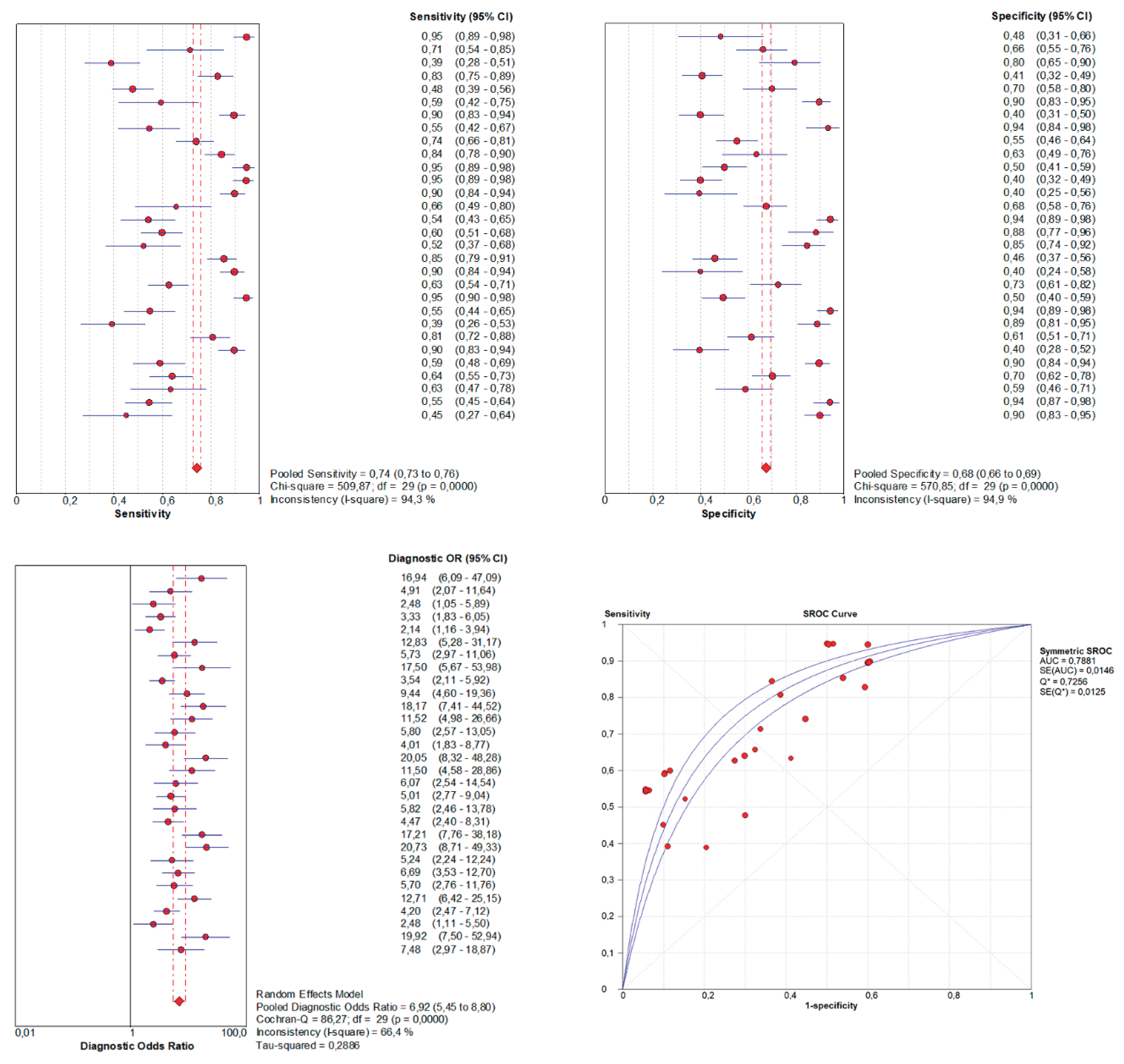
Figure 2.
Hierarchical meta-analysis of the same simulated dataset was performed using Stata. The upper panel displays a forest plot of sensitivity and specificity, jointly modeled within the bivariate framework (generated with metadta). The lower panel shows hierarchical summary receiver operating characteristic (HSROC) curves generated using three different Stata commands: metandi (left), metadta (center), and midas (right). Although the three approaches yield broadly similar point estimates of summary sensitivity and specificity—reflecting their shared BRMA foundation—this apparent agreement should not be interpreted as full methodological equivalence. As discussed in the main text, important differences remain in how prediction regions, heterogeneity, and overall accuracy metrics (e.g., AUC) are estimated, with implications for uncertainty and clinical interpretation. Each dot represents an individual study's estimate of sensitivity and specificity; in the metandi plot, circle size is proportional to the study's sample size. Both metandi and metadta fit the BRMA model, from which they derive HSROC parameters and curves through re-parameterization (reflecting the equivalence between BRMA and HSROC formulations). In contrast, midas generates the ROC curve as a continuous extrapolation derived from the bivariate model output, rather than through formal HSROC modeling, which results in a complete inferential ROC curve extending across the entire 0–1 specificity range. All three commands generate an elliptical confidence region (uncertainty around the summary estimate) and a prediction region (expected range of future studies). It is noteworthy that the prediction region generated by midas appears substantially wider than those produced by metandi and metadta, consistent with the methodological reasons discussed in the main text (i.e., midas ignores the covariance between logit-sensitivity and logit-specificity when constructing the prediction ellipse, leading to inflated dispersion). Lastly, the visual distribution of individual studies follows an ascending pattern along the ROC space, consistent with the expected inverse relationship between sensitivity and specificity due to threshold variability. This alignment suggests that differences in positivity thresholds across studies may partially explain the observed dispersion.
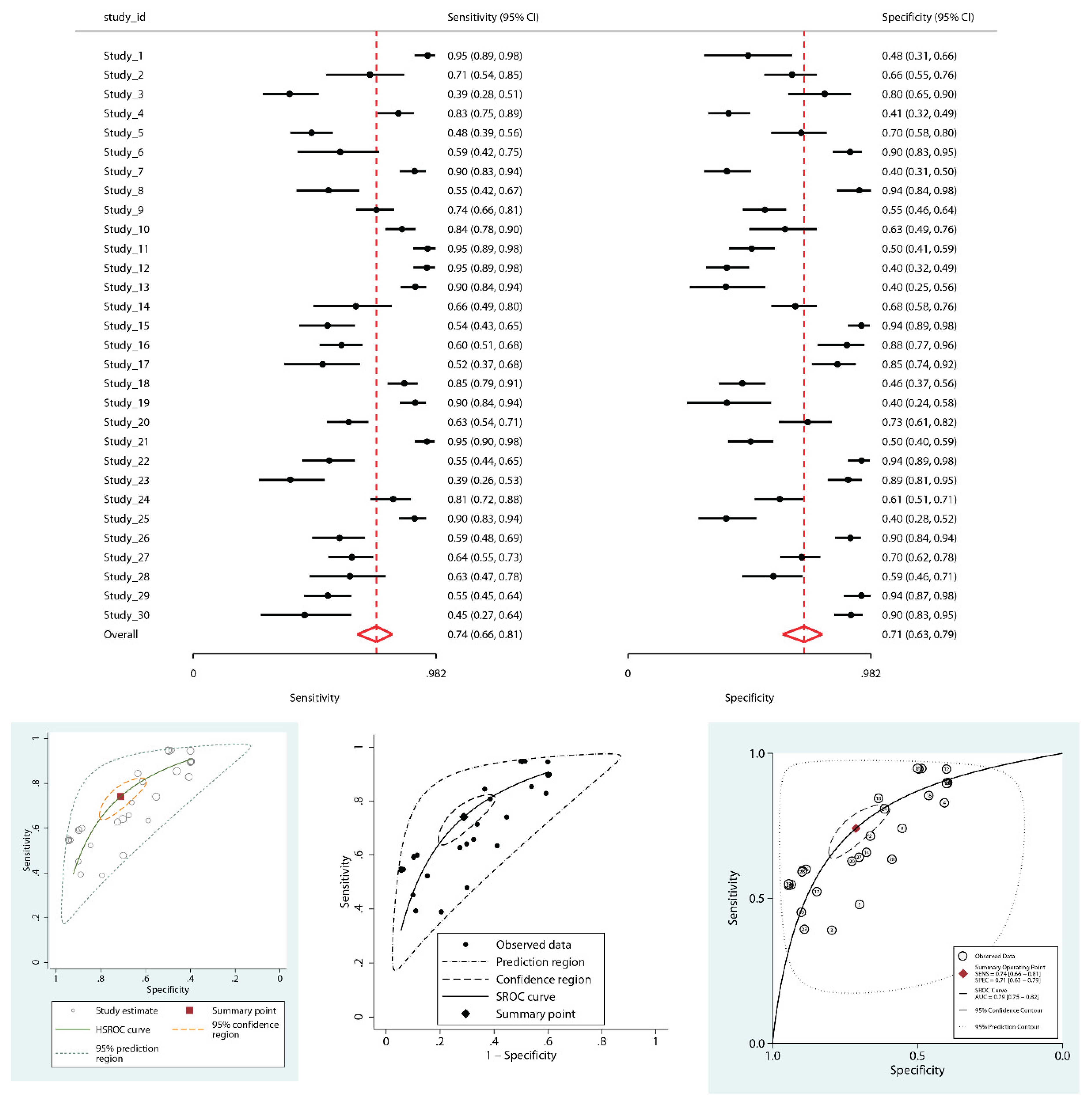

Table 1.
Comparative features of Stata commands for meta-analysis of diagnostic test accuracy.
| Feature | metandi (Harbord & Whiting, 2009) | midas (Dwamena, 2007) | metadta (Nyaga & Arbyn, 2022) |
|---|---|---|---|
| Primary Model | BRMA only. HSROC parameters/curve derived from BRMA output (not a separately fitted HSROC model). | BRMA only. ROC curve is an indirect approximation derived from the BRMA output, not a formal HSROC model. | BRMA (bivariate framework); HSROC curve obtained via formal re-parameterization (mathematically equivalent to Rutter & Gatsonis). |
| Meta-Regression | Not supported. | Univariable only. Cannot fit multivariable models. | Supports both Univariable and Multivariable meta-regression. |
| Heterogeneity Metrics | Reports between-study variance components (τ²). Does not calculate a bivariate I² statistic. | Reports univariate I² statistics, ICCs for sensitivity and specificity, and median sensitivity/specificity estimates. Does not calculate between-study variance components (τ²) | Reports between-study variance (τ²) and the bivariate I² (Zhou) |
| Influence Diagnostics | Supported via the predict post-estimation command to obtain Cook's distance and standardized residuals. | Supported via the integrated modchk option, which generates a panel of four diagnostic plots. | No built-in commands for influence diagnostics. Requires manual post-estimation calculations. |
| Publication Bias Test | Not supported. | Supported via the pubbias subcommand, which implements the recommended Deeks' test. | Not supported. |
| Clinical Utility Tools | Not supported. | Provides Fagan nomograms, a likelihood ratio scattergram, a bivariate boxplot for outlier detection, and calculates the diagnostic odds ratio (DOR). | Not supported. |
| Graphical Output | Generates a formal HSROC plot with correctly calculated confidence and prediction regions. | Generates an approximate ROC plot, Fagan nomograms, and various other diagnostic plots. | Generates high-quality forest plots and an HSROC plot with correctly calculated confidence and prediction regions. |
| Key Limitation | Lacks meta-regression and many modern analytical features. Can be prone to model convergence issues, especially with sparse data or zero-events. | The prediction region is methodologically flawed and inflated due to ignoring covariance. The reported AUC is an extrapolation based on untestable assumptions. | Lacks built-in functions for publication bias assessment and influence diagnostics, requiring the use of other packages (like midas) to complete a full analysis. |
BRMA = bivariate random-effects meta-analysis (Reitsma model); HSROC = hierarchical summary receiver operating characteristic model (Rutter & Gatsonis); τ² = between-study variance; I² = heterogeneity statistic; ICC = intraclass correlation coefficient; Se = sensitivity; Sp = specificity; DOR = diagnostic odds ratio; LR = likelihood ratio; AUC = area under the curve; ρₐᵦ (rho) = correlation coefficient between sensitivity and specificity; ROC = receiver operating characteristic.
Table 2.
Conceptual and methodological differences between traditional and hierarchical meta-analytical models for diagnostic test accuracy.
Table 2.
Conceptual and methodological differences between traditional and hierarchical meta-analytical models for diagnostic test accuracy.
| Aspect | Traditional Models (DerSimonian-Laird, Moses-Littenberg) | Hierarchical Models (HSROC, BRMA) |
|---|---|---|
| Software Availability | Multiple platforms, including outdated tools: MetaDisc 1.4, RevMan 5.4, Stata, R, SAS. | Stata, R, Meta-DiSc 2.0 (limited but specific support). |
| Reported Metrics | Sensitivity and specificity (analyzed separately), symmetric ROC curve, DOR. | Joint modeling of sensitivity and specificity, LR+, LR–, DOR; hierarchical ROC curve (data-restricted); AUC estimated in select cases. |
| Confidence Intervals | Often narrow and symmetric, prone to underestimating uncertainty. | Data-dependent, typically wider and asymmetric, better reflect true variability. |
| Heterogeneity Assessment | Cochran's Q and I² statistics (may misrepresent variability due to inability to disentangle threshold and non-threshold heterogeneity). | Bivariate I² (Zhou), variance estimates for sensitivity and specificity, prediction regions for visual assessment. |
| Threshold Effect Handling | Ignored; assumes a common threshold across studies, may distort pooled estimates. | Models threshold heterogeneity by allowing study-specific operating points via random effects; HSROC separates accuracy and threshold components. A negative Se–Sp correlation often arises under threshold variability but is a consequence, not the mechanism |
| Interpretation of ROC Curve | Assumes a symmetric ROC curve as a mathematical simplification, which may not reflect the true asymmetry or variability present in empirical data. The curve is often extrapolated beyond the observed data range. | The ROC curve is typically constrained to the empirical data range, incorporating asymmetry, threshold effects, and between-study heterogeneity. Best practice is to display the HSROC primarily over the observed operating range to avoid misleading extrapolation; extrapolation is a plotting choice, not a model property |
| Summary Estimates Robustness | Pooled estimates (Se, Sp, DOR) are often misleading when there is high heterogeneity. | Summary points and prediction regions account for between-study variability and correlation. |
| Advanced Diagnostics | Not available. | Influence diagnostics (Cook's distance, standardized residuals), bivariate boxplots, LR+ and LR- scattergrams, model fit assessment. |
| Meta-Regression | Not available. | Available (univariable and multivariable). |
| Outlier Detection and Robustness | Limited capacity. | Systematic outlier identification supports sensitivity analyses and model refinement. |
| Publication Bias Assessment | Begg's test, Egger's regression, funnel plots (limited validity for DTA) | Deeks' test (specifically designed for DTA). |
| Study-Level Variance Handling | Often underestimated; ignores study clustering. | Explicit variance modeling for sensitivity and specificity; accounts for within- and between-study variability. |
HSROC: Hierarchical summary receiver operating characteristics model (Rutter and Gatsonis); BRMA: Bivariate random effects model (Reitsma); Se: Sensitivity; Sp: Specificity; DOR: Diagnostic odds ratio; DTA: Diagnostic test accuracy meta-analysis.
Table 3.
Key Take-Home Messages for Conducting DTA Meta-Analyses.
| Recommendation | Rationale | Practical Implication |
|---|---|---|
| Plan and report analyses transparently | Post hoc choices increase the risk of bias and reduce reproducibility | Best practice includes protocol registration (e.g., PROSPERO) and reporting per PRISMA-DTA, with all statistical analyses pre-specified in the protocol |
| Mandate hierarchical models (BRMA/HSROC) | Separate pooling ignores correlation and underestimates uncertainty | Always apply hierarchical models (BRMA/HSROC) as the gold standard; avoid separate pooling approaches that ignore threshold effects and heterogeneity |
| Select appropriate software | Not all platforms support hierarchical modelling or advanced diagnostics | Use Stata (metandi/metadta/midas) or R (mada/diagmeta). MetaDisc 2.0, although more limited, allows hierarchical modelling |
| Report paired Se and Sp, LR+/– and CI/prediction regions | Se or Sp alone mask trade-offs and should not be analyzed separately | Always show sens/spec with 95% CI, plus LR+ and LR–; add joint CI/prediction regions |
| Use AUC and DOR cautiously | AUC extrapolates beyond observed data; DOR has limited interpretability | If reported, include CIs and note limitations; prioritize primary metrics (Se, Sp, LR+, LR-) |
| Quantify heterogeneity with τ² and bivariate I² | Univariate I² exaggerates heterogeneity in DTA | Report τ² for sens/spec and Zhou’s bivariate I²; interpret in context |
| Assess threshold effects | Negative correlation (ρₐᵦ) indicates threshold-driven heterogeneity | Report and interpret ρₐᵦ |
| Perform influence and sensitivity analyses | Outliers distort pooled estimates and heterogeneity | Use Cook’s distance, residuals, and bivariate boxplots to identify influential studies. Report the primary analysis with all studies, and then provide a transparent sensitivity analysis excluding them. The purpose is to test robustness, not to replace the primary result |
| Assess publication bias | Egger/Begg are invalid for DTA; Deeks is recommended only if ≥10 studies | Apply Deeks’ with caution; discuss small-study effects and low power |
| Consider performing meta-regression | Pre-specify covariates and modeling strategy; avoid post-hoc DTA dredging. Data-driven dichotomization inflates Type I error and biases effect estimates. | Model continuous covariates on their natural scale; treat findings as exploratory unless pre-planned and adequately powered (≈≥10 studies per covariate). |
| Use complementary graphical tools | Graphical outputs enhance clinical applicability | Include HSROC curves, Fagan nomograms, and LR scatterplots |
HSROC: Hierarchical summary receiver operating characteristics model (Rutter and Gatsonis); BRMA: Bivariate random effects model (Reitsma); Se: Sensitivity; Sp: Specificity; DOR: Diagnostic odds ratio; DTA: Diagnostic test accuracy meta-analysis; LR: likelihood ratio; τ² (tau-squared): between-study variance; ρₐᵦ (rho): correlation coefficient between sensitivity and specificity.
Disclaimer/Publisher’s Note: The statements, opinions and data contained in all publications are solely those of the individual author(s) and contributor(s) and not of MDPI and/or the editor(s). MDPI and/or the editor(s) disclaim responsibility for any injury to people or property resulting from any ideas, methods, instructions or products referred to in the content. |
© 2025 by the authors. Licensee MDPI, Basel, Switzerland. This article is an open access article distributed under the terms and conditions of the Creative Commons Attribution (CC BY) license (http://creativecommons.org/licenses/by/4.0/).
Copyright: This open access article is published under a Creative Commons CC BY 4.0 license, which permit the free download, distribution, and reuse, provided that the author and preprint are cited in any reuse.


