
Submitted:
20 October 2025
Posted:
21 October 2025
You are already at the latest version
Abstract
Meta-analysis has become a routine component of clinical research, but the software used to conduct it strongly influences how evidence is modelled, interpreted, and translated into practice. This article provides a practical field guide to modern meta-analysis software, explaining how to choose, justify, and implement current methodological standards in day-to-day work. Rather than critiquing outdated tools, the tutorial shows what applied researchers should do to produce analyses that are robust, transparent, and reproducible. The guide distinguishes legacy platforms (RevMan 5.4, MetaDiSc 1.4, Comprehensive Meta-Analysis) from modern implementations (RevMan Web, MetaDiSc 2.0, and script-based solutions such as R and Stata), clarifying which defaults matter, why certain estimators and models have been superseded, and how hierarchical and likelihood-based approaches improve real-world inference. Short, software-agnostic explanations outline when REML or Paule–Mandel estimators are preferable to DerSimonian–Laird, when Hartung–Knapp adjustments are warranted, and why diagnostic accuracy meta-analysis requires bivariate or HSROC models rather than separate pooling of sensitivity and specificity. By positioning software choices within the logic of the modelling workflow, this tutorial enables readers to anticipate limitations, justify methodological decisions, and avoid silent defaults that weaken inference. The objective is not merely technical update but conceptual alignment: treating meta-analysis as a modelling exercise requiring transparency and judgment rather than a mechanical point-and-click task. This field guide is intended as a practical resource for authors, reviewers, and journals aiming to raise methodological standards in applied evidence synthesis.
Keywords:
RevMan 5.4
; Meta-DiSc1.4
; comprehensive meta-analysis
; REML
; HSROC
; bivariate
; Moses-Littenberg
; Wald-type intervals
; Hartung–Knapp–Sidik–Jonkman adjustment
Introduction
Meta-analysis occupies a central role in evidence-based medicine [1,2], but the way it is implemented in practice depends heavily on the statistical estimation defaults and model constraints embedded in software. These estimation defaults and model constraints determine how heterogeneity is estimated, how uncertainty is expressed, and whether the model reflects a single pooled effect or a distribution of effects across settings. Understanding the progression from DerSimonian–Laird estimators [3] toward likelihood-based approaches such as REML [4,5] or Paule–Mandel [6,7], from traditional Wald-type intervals [3] toward Hartung–Knapp–Sidik–Jonkman adjustments [8,9,10,11,12,13,14], and from Moses–Littenberg models [15] toward hierarchical bivariate [16] or HSROC models [17,18], is therefore a prerequisite for selecting appropriate software rather than a purely historical detail.
The continued use of legacy software does not stem from its methodological superiority, but from historical accessibility and workflow familiarity [19]. Earlier programs became widely adopted because they were free, intuitive, or officially endorsed, while commercial alternatives offered a low-entry path for applied researchers who were unfamiliar with code-based solutions. Modern platforms provide stronger estimators and broader functionality, but are perceived as requiring additional statistical literacy or licensing, which delays their routine adoption despite methodological advantages. This tutorial addresses that gap pragmatically: by clarifying which defaults matter and how to implement the recommended methods in practice, it enables readers to transition from legacy tools to reproducible, likelihood-based frameworks without assuming prior expertise.
Meta-analysis is not a routine calculation but a modelling framework that requires explicit choices about variance estimation, uncertainty, and generalisability. Software mediates those choices: when defaults remain implicit, the rationale behind a model is lost and interpretation becomes difficult to justify. Point-and-click interfaces lowered barriers to entry, but also separated users from the underlying modelling logic, which makes it harder to understand when a different estimator, interval method, or framework is warranted. This tutorial addresses that gap by linking the statistical model to the software features that implement it, helping readers interpret outputs as modelling decisions rather than automated results. The emphasis is therefore not on replacing one program with another, but on recognising how software encodes assumptions and how to select tools that make those assumptions explicit.
The practical implication of these hidden defaults is that key modelling choices — such as how τ² is estimated, how uncertainty is expressed, or whether studies with zero events are retained or excluded — often remain implicit rather than explicitly justified. When these decisions are surfaced and understood, software choice becomes part of the modelling rationale instead of a background constraint. The purpose of this tutorial is therefore not only to describe the evolution of meta-analytic software, but to equip readers with a framework for recognising which defaults matter, how to override or justify them, and how to align implementation with contemporary methodological standards.
To support this shift in practice, the remainder of this article is structured as a step-by-step guide linking software platforms to the modelling principles they implement. First, it reviews how legacy programs encode historical defaults and why these matter for inference. It then outlines the modern implementations that operationalise likelihood-based and hierarchical models, before providing a practical roadmap for selecting, justifying, and reporting software choices in applied meta-analytic work. In doing so, the article repositions software selection as part of methodological reasoning rather than a procedural detail.
How Software Determines the Model: From Legacy Defaults to Modern Standards
Review Manager (RevMan): A Tale of Two Versions
RevMan, the flagship software of Cochrane, exemplifies the challenge of methodological transition. For decades, its desktop version, RevMan 5.4, was the most widely used tool for systematic reviews, largely due to its accessibility and official endorsement. However, its statistical engine is now profoundly outdated.
- For intervention reviews, RevMan 5.4 [20] defaults to the DL estimator for random-effects models— a built-in constraint of the software, rather than an optional setting a user can modify. The dominance of the DL estimator did not arise arbitrarily: its computational simplicity and early endorsement facilitated widespread adoption. In scenarios with a large number of studies and low heterogeneity, its performance is often comparable to more advanced estimators. Simulation studies show that when the number of studies is small or heterogeneity is substantial, DL tends to underestimate τ², which results in narrower confidence intervals than intended. This behaviour is not an implementation flaw but a statistical property of the estimator, and it is the reason why likelihood-based alternatives such as REML are preferred when modelling heterogeneity is clinically relevant. More robust alternatives such as REML or PM are absent in RevMan 5.4, as are HKSJ adjustments that correct the well-documented deficiencies of Wald-type intervals. Prediction intervals—now considered essential for interpreting clinical heterogeneity—are also not provided. Even the graphical outputs are problematic: forest plots often apply a confusing label, “M-H, Random,” which reflects the use of Mantel–Haenszel weights in the heterogeneity statistic prior to DL estimation, but is frequently misinterpreted as a literal hybrid model. The Mantel-Haenszel (MH) method is a fixed-effect approach by definition, yet the software applies the DL random-effects estimator, creating a significant source of confusion for users.
- In diagnostic test accuracy (DTA) reviews, RevMan does not internally estimate bivariate or HSROC models; instead, it treats sensitivity and specificity as separate outcomes and fits a Moses–Littenberg SROC by default. While this interface can display parameters from a hierarchical model if supplied externally, the software itself does not perform the hierarchical estimation. This means that in RevMan, the user selects the framework indirectly through the software’s capabilities rather than through an explicit modelling choice. This approach systematically overstates accuracy compared with hierarchical models [18], because it assumes a symmetric SROC and treats the regression slope as a threshold effect.
Beyond these domain-specific flaws, RevMan lacks the flexibility to fit meta-regression models with modern estimators, to conduct advanced sensitivity analyses, or to generate outputs compatible with transparent reproducibility. More sophisticated approaches, such as Bayesian modeling, network meta-analysis, or hierarchical frameworks for complex data structures, are entirely unavailable.
This creates a practical lag between methodological guidance and routine implementation: although current Cochrane standards recommend likelihood-based estimators and hierarchical models, many published reviews still reflect the specifications of the earlier software environment. The resulting pattern is less a matter of resistance than of tooling inertia — users adopt the capabilities of the platform available to them, and upgrading the model often requires upgrading the software.
In a major and timely update, Cochrane has expanded the statistical framework in RevMan Web (version 7), addressing several core limitations of its predecessor and aligning its default estimators with current methodological guidance [21].
- Robust Default Estimator: The default estimator for τ2 is now REML, with DL remaining as a user-selectable option.
- HKSJ Confidence Intervals: The HKSJ adjustment is now available for calculating CIs for the summary effect, providing better coverage properties than traditional Wald-type intervals.
- Prediction Intervals: The software now calculates and displays prediction intervals on forest plots, enhancing the interpretation of heterogeneity by showing the expected range of effects in future studies.
RevMan Web represents a substantial methodological improvement over version 5.4, but its functionality remains bounded by the capabilities of its statistical engine. The platform does not implement user-defined estimators or likelihood specifications, and advanced workflows such as network meta-analysis, Bayesian modelling, or custom meta-regression still require script-based environments such as R or Stata. For diagnostic test accuracy, RevMan Web can display parameters from hierarchical models but does not estimate them internally, as it continues to treat sensitivity and specificity as separate outcomes. These constraints do not affect the validity of its standard outputs, but they limit its role to conventional intervention meta-analysis and make it unsuitable for settings where model specification must be explicitly controlled by the analyst.
MetaDiSc 1.4 vs 2.0: Modelling Frameworks Compared
MetaDiSc 1.4 was a pioneering free tool for DTA meta-analysis [22], which explains its historical persistence. However, it implements a univariate modelling approach in which sensitivity and specificity are pooled as separate, uncorrelated metrics, and it uses the Moses–Littenberg framework to construct the summary ROC curve. This model does not account for the joint distribution of sensitivity and specificity or for between-study variability in threshold effects.
In 2022, a web-based successor, MetaDiSc 2.0 [23], was released. The new version correctly implements the current gold standard for DTA synthesis:
- Bivariate Hierarchical Model: MetaDiSc 2.0 uses a hierarchical random-effects model as its core engine, modelling sensitivity and specificity as a correlated pair, which more accurately reflects how test performance varies across study populations and settings.
- Confidence and Prediction Regions: The software generates both a 95% confidence region for the summary point (quantifying uncertainty in the mean estimate) and a 95% prediction region (illustrating the expected range of true accuracy in a future study).
This update makes MetaDiSc 2.0 a methodologically appropriate tool for standard DTA meta-analyses. While it does not include advanced features such as hierarchical meta-regression or user-specified likelihoods, its implementation of the bivariate model aligns it with current methodological standards for conventional diagnostic accuracy synthesis.
Although version 2 is available, many researchers continue to use MetaDiSc 1.4, largely because it is historically cited in methodological literature and remains widely accessible online. Version 1.4 implements separate pooling of sensitivity and specificity and uses the Moses–Littenberg approach for constructing the SROC curve, which does not account for their correlation or for threshold-related between-study variability. As a result, it cannot produce hierarchical summaries or confidence and prediction regions that reflect the full joint distribution of diagnostic performance.
Comprehensive Meta-Analysis: Closed-Code Estimation and Default Constraints
Comprehensive Meta-Analysis (CMA) is a widely used commercial program with a user-friendly graphical interface. Version 3 became the most widely used release [24,25], supported by manuals, tutorials, and extensive applied literature. Its relatively low licensing cost and interface design made it accessible to clinicians and applied researchers at a time when script-based workflows were less common, which explains its broad uptake.
However, CMA is a closed-code environment: the underlying algorithms and variance formulas are not publicly documented, and the choice of estimator cannot be inspected or modified by the user. Methodological reviews indicate that CMA3 relies on the DerSimonian–Laird estimator for random effects [26], does not provide REML or Paule–Mandel options, does not implement HKSJ adjustments, and does not calculate prediction intervals. These constraints do not affect usability, but they limit the modelling framework to default methods that may underestimate heterogeneity in settings with few studies or substantial between-study variability. Meta-regression is available but remains less flexible than in script-based software.
Although CMA version 4 was released in 2023 [27], publicly available documentation still refers primarily to version 3, and it remains unclear whether the estimation engine has been updated. The absence of transparent documentation means that the statistical framework must be inferred indirectly from interface behaviour and independent evaluations rather than from verifiable specifications. As a result, CMA is suitable for users who prioritise accessibility over custom modelling, whereas workflows requiring explicit control over estimators, likelihoods, or hierarchical structures still necessitate open, script-based platforms.
A comparative overview of the main software platforms, their accessibility, requirements, and current limitations is provided in Table 1. Figure 1 presents a chronological overview of software developments for meta-analysis, tracing the shift from early, limited programs to more recent platforms. The timeline highlights how successive releases have progressively expanded methodological options and transparency.
Current Methodological Standards For Meta-Analytic Modelling (Intervention Reviews)
Modeling (Estimator)
Random-effects models should be fitted using likelihood-based estimators of between-study variance, most commonly REML or PM [1]. These approaches provide more stable estimation of τ² than method-of-moments estimators such as DL, particularly when heterogeneity is non-trivial or the number of studies is small. Between the two, REML is generally preferred because PM may produce upwardly biased estimates of τ² when study sample sizes are highly unbalanced [6,7]. Accordingly, REML is typically recommended for general use, while PM remains a reasonable alternative when study designs are more homogeneous.
Confidence Intervals and Prediction Intervals
For confidence intervals, two complementary approaches are commonly used. WT intervals are widely implemented, but they do not incorporate the uncertainty in the estimation of τ². The HKSJ method (Hartung–Knapp–Sidik–Jonkman) incorporates this uncertainty and therefore tends to provide more reliable coverage when between-study variability is present. In situations where τ² is very small or the number of studies is limited (e.g., k < 5), a modified version of this method (mHK) is available to stabilise the interval width and avoid excessive broadening under near-zero heterogeneity [28].
For meta-analyses with more than two studies and τ² > 0, HKSJ-adjusted intervals are generally preferred [1]. When only a small number of studies is available, it can be helpful to present both REML WT and REML HKSJ intervals to illustrate how explicitly modelling τ² uncertainty affects precision [1]. In all cases, prediction intervals should also be reported to describe the expected range of effects in new or future populations, supporting clinical interpretation.
Heterogeneity
Heterogeneity should be evaluated using measures that reflect both its magnitude and its implications for interpretation. Because I² is influenced by the number of included studies and does not express absolute variability, it is informative but not sufficient on its own. Reporting τ² together with its confidence interval, and examining the forest plot, provides a more direct summary of between-study variance [1]. Prediction intervals can further contextualise this variability by illustrating how effect estimates may differ in future settings. Sensitivity analyses assessing the influence of individual studies or design features are also useful, and where appropriate, meta-regression with robust estimators can help explore potential sources of heterogeneity [1].
Current Methodological Standards For Meta-Analytic Modelling (Diagnostic Test Accuracy Reviews)
Modeling (Estimator)
Diagnostic test accuracy meta-analyses should be fitted using hierarchical models that jointly estimate sensitivity and specificity, rather than analysing them separately [29,30,31,32]. The bivariate random-effects model and the HSROC model are the recommended approaches [2], as both account for within- and between-study variability and the correlation between sensitivity and specificity. These frameworks also allow threshold effects to be represented explicitly, which is important when positivity criteria vary across studies — a feature not accommodated by earlier univariate methods such as Moses–Littenberg [2,15].
Confidence Regions and Prediction Regions
In DTA synthesis, uncertainty is conveyed through regions rather than single-dimension intervals. Confidence regions describe the uncertainty of the pooled summary point, while prediction regions illustrate how diagnostic performance may vary in new or external populations. Reporting both provides a fuller representation of test accuracy, combining precision around the estimate with its dispersion across likely practice conditions [2].
Heterogeneity
Heterogeneity in DTA arises from differences in populations, thresholds, study design, or test interpretation. Hierarchical models address this by allowing random effects for both sensitivity and specificity and by modelling their correlation and threshold behaviour [2]. Univariate metrics such as separate I² values for sensitivity and specificity do not capture this joint structure and may misrepresent variability. More informative summaries include the estimated variances of sensitivity and specificity together with their covariance (or threshold effect), such as the Zhou bivariate measure [33]. Beyond model-based variance components, heterogeneity can also be explored through subgroup analyses, meta-regression, and visual inspection of the SROC, with prediction regions providing additional context for expected variation in real-world practice.
Figure 2 summarises the principal milestones in the development of statistical methodology for meta-analysis, tracing the progression from early variance estimators toward hierarchical and likelihood-based approaches. The timeline illustrates how successive innovations expanded modelling capabilities and improved the treatment of heterogeneity and uncertainty in applied synthesis.
How Software Choice Shapes Inference in Practice
The continued use of older meta-analysis software reflects historical adoption patterns rather than methodological preference. When platforms implement method-of-moments estimators such as DL or do not provide prediction intervals, the resulting models represent uncertainty differently than likelihood-based approaches. These differences originate from how variability is estimated and expressed, not from the data themselves. In diagnostic accuracy reviews, the use of univariate frameworks such as Moses–Littenberg produces summary curves that do not incorporate between-study variability or the correlation between sensitivity and specificity, which leads to less informative characterisations of performance. Understanding the modelling framework is therefore essential for interpreting what a pooled estimate does—and does not—represent.
Even when robust estimators are used, a random-effects model summarises an average across heterogeneous studies, which may not reflect the range of effects observed in distinct clinical settings. As highlighted in the causal inference literature [34], pooled estimates describe the evidence base under the included study conditions and may not automatically transport to new populations. For this reason, interpretation requires attention not only to the point estimate but also to the dispersion of effects across plausible contexts.
Reproducibility is also influenced by software design. Closed or menu-restricted environments limit the extent to which modelling assumptions can be inspected, modified, or replicated externally. When the underlying code or estimation procedures are not visible, independent validation becomes more difficult, and analytical choices remain implicit rather than explicitly justified. Recognising these constraints frames software selection as part of methodological reasoning rather than a procedural detail.
Specific modelling behaviours attributable to legacy platforms, together with the corresponding recommended alternatives, are summarised in Table 2. Building on this, Table 3 provides practical guidance on how to select and transparently report software and estimators in a way that aligns the modelling goals with their implementation.
Hidden Estimation Rules: Continuity Corrections and Automatic Exclusions
Legacy software often applies continuity corrections or automatic study exclusions without explicitly reporting them in the output. These operations are intended to ensure model estimability in sparse-data settings, but they remain invisible to the user and can therefore influence interpretation without being recognised as modelling choices. In RevMan 5.4, for example, a fixed zero-cell adjustment—equivalent to a modified Haldane–Anscombe (mHA) correction of 0.5—is applied by default, and studies with zero events in both arms are excluded when ratio measures are used [35]. The correction is not selectable or reported in the interface, which makes it difficult for readers to determine how the estimates were obtained.
Alternative approaches allow these studies to be retained rather than dropped—for example, the Carter correction, which adds one event and two participants per arm—preserving estimability while avoiding automatic exclusions [36]. None of these strategies is inherently superior in all circumstances; what distinguishes them is whether the adjustment is transparent and whether users are able to justify it in light of the review context. In rare-event meta-analysis, visibility of the modelling step is therefore essential for reproducibility and interpretation.
Implementation Guidance for Authors, Reviewers, and Editors
The older software platforms discussed earlier played an important historical role in the uptake of meta-analysis, but their estimation engines reflect earlier methodological conventions. Contemporary tools—whether RevMan Web [21,37], MetaDiSc 2, or script-based environments such as R and Stata—provide greater transparency, allow explicit model specification, and support likelihood-based or hierarchical estimation. Transitioning to these platforms aligns implementation with current methodological standards.
For authors: Reporting should specify which estimator of τ² was used (e.g., DL, REML, PM) and, where relevant, how uncertainty was quantified (WT vs HKSJ/mHK). Explicit justification of the chosen estimator facilitates interpretability and allows readers to understand the modelling assumptions that underpin the pooled estimate.
For journal editors: Requiring the explicit reporting of τ² estimators and interval methods would increase transparency and make analytical decisions auditable. This step does not prescribe a single “correct” model but ensures that the modelling framework is visible to the reader.
For peer reviewers: When DL is used by default—particularly with a small number of studies—it is helpful to request sensitivity analyses using REML or PM, and to consider whether prediction intervals or HKSJ adjustments are appropriate. The goal is not to enforce a specific method but to assess whether inference is robust to alternative estimators.
For training programs and institutions: Teaching meta-analysis as a modelling exercise rather than a menu-driven procedure better reflects current standards. Script-based platforms provide a transparent environment in which modelling assumptions are explicit, reproducible, and modifiable.
Meta-analysis informs guidelines, policy, and clinical decision-making; therefore, clarity about how the model is estimated enhances the interpretability and applicability of results. Reform in this context means aligning analytical tools with contemporary methodology and ensuring that the underlying modelling decisions are transparent rather than implicit.
Conclusions
Meta-analysis is a modelling framework in which validity depends on how variance is estimated, how uncertainty is expressed, and how results are interpreted in context. The software used to implement the analysis determines which models can be specified and which defaults govern estimation. Aligning practice with contemporary methodology therefore involves making those modelling choices explicit—both in terms of estimator selection and in the reporting of interval and prediction structures. Robust estimators, hierarchical models, and transparent reporting enhance interpretability, support reproducibility, and facilitate appropriate application of results in clinical and policy settings. In this way, software choice becomes part of methodological reasoning rather than a procedural detail, strengthening the credibility of evidence synthesis.
Original work
The manuscript’s author declares that it is an original contribution, not previously published.
Informed consent
N/A
AI Use Disclosure
Artificial intelligence (ChatGPT-4, OpenAI) was used to improve the clarity and style of the language
Ethical Statement
This study did not involve human subjects or animals. As only simulated data were used, no ethical approval or informed consent was required.
Data Availability Statement
No new datasets were generated or analyzed for the purposes of this work.
Conflict of interest
There is no conflict of interest or external funding to declare. The author does not have anything to disclose
References
- Higgins JPT, Thomas J, Chandler J, Cumpston M, Li T, Page MJ, Welch VA (editors). Cochrane Handbook for Systematic Reviews of Interventions version 6.5 (updated August 2024). Cochrane, 2024. Available from www.cochrane.org/handbook.
- Deeks JJ, Bossuyt PM, Leeflang MM, Takwoingi Y (editors). Cochrane Handbook for Systematic Reviews of Diagnostic Test Accuracy. Version 2.0 (updated July 2023). Cochrane, 2023. Available from https://training.cochrane.org/handbook-diagnostic-test-accuracy/current.
- DerSimonian R, Laird N. Meta-analysis in clinical trials. Control Clin Trials. 1986 Sep;7(3):177-88. [CrossRef] [PubMed]
- Viechtbauer, W. (2005). Bias and Efficiency of Meta-Analytic Variance Estimators in the Random-Effects Model. Journal of Educational and Behavioral Statistics, 30(3), 261-293. [CrossRef]
- Veroniki AA, Jackson D, Viechtbauer W, Bender R, Bowden J, Knapp G, et al. Methods to estimate the between-study variance and its uncertainty in meta-analysis. Res Synth Methods. 2016;7(1):55–79. [CrossRef]
- Paule RC, Mandel J. Consensus values and weighting factors. J Res Nat Bur Stand. 1982;87(5):377--385. [CrossRef]
- van Aert RCM, Jackson D. Multistep estimators of the between-study variance: The relationship with the Paule-Mandel estimator. Stat Med. 2018 Jul 30;37(17):2616-2629. [CrossRef] [PubMed]
- Hartung, J. An alternative method for meta--analysis. Biom J. 1999;41(8):901--916.
- Hartung J, Knapp G. On tests of the overall treatment effect in meta--analysis with normally distributed responses. Stat Med. 2001;20(12):1771--1782. [CrossRef]
- Hartung J, Knapp G. A refined method for the meta--analysis of controlled clinical trials with binary outcome. Stat Med. 2001;20(24):3875--3889. [CrossRef]
- Sidik K, Jonkman JN. A simple confidence interval for meta--analysis. Stat Med. 2002;21(21):3153--3159. [CrossRef]
- IntHout, J. , Ioannidis, J.P. & Borm, G.F. The Hartung-Knapp-Sidik-Jonkman method for random effects meta-analysis is straightforward and considerably outperforms the standard DerSimonian-Laird method. BMC Med Res Methodol 14, 25 (2014). [CrossRef]
- Röver, C. , Knapp, G. & Friede, T. Hartung-Knapp-Sidik-Jonkman approach and its modification for random-effects meta-analysis with few studies. BMC Med Res Methodol 15, 99 (2015). [CrossRef]
- Langan D, Higgins JPT, Jackson D, Bowden J, Veroniki AA, Kontopantelis E, Viechtbauer W, Simmonds M. A comparison of heterogeneity variance estimators in simulated random-effects meta-analyses. Res Synth Methods. 2019 Mar;10(1):83-98. [CrossRef] [PubMed]
- Moses LE, Shapiro D, Littenberg B. Combining independent studies of a diagnostic test into a summary ROC curve: data-analytic approaches and some additional considerations. Stat Med 1993;12:1293-316. [CrossRef]
- Reitsma JB, Glas AS, Rutjes AWS, Scholten RJPM, Bossuyt PM, Zwinderman AH. Bivariate analysis of sensitivity and specificity produces informative summary measures in diagnostic reviews. J Clin Epidemiol, 2005; 58, 10, 982e90. [CrossRef]
- Rutter CM, Gatsonis CA. A hierarchical regression approach to meta-analysis of diagnostic test accuracy evaluations. Stat Med. 2001 Oct 15;20(19):2865-84. [CrossRef] [PubMed]
- The Moses-Littenberg meta-analytical method generates systematic differences in test accuracy compared to hierarchical meta-analytical models. J Clin Epidemiol. 2016 Dec;80:77-87. [CrossRef] [PubMed]
- Wang J, Leeflang M. Recommended software/packages for meta-analysis of diagnostic accuracy. J Lab Precis Med 2019;4:22. [CrossRef]
- Review Manager 5 (RevMan 5) [Computer program]. Version 5.4. Copenhagen: The Cochrane Collaboration, 2020.
- Review Manager (RevMan) [Computer program]. Version 7.2.0. The Cochrane Collaboration, 2024. Available at revman.cochrane.org.
- Zamora J, Abraira V, Muriel A, Khan K, Coomarasamy A. Meta-DiSc: a software for meta-analysis of test accuracy data. BMC Med Res Methodol. 2006 Jul 12;6:31. [CrossRef] [PubMed]
- Plana, M.N. , Arevalo-Rodriguez, I., Fernández-García, S. et al. Meta-DiSc 2.0: a web application for meta-analysis of diagnostic test accuracy data. BMC Med Res Methodol 22, 306 (2022). [CrossRef]
- Brüggemann, P. , Rajguru, K. Comprehensive Meta-Analysis (CMA) 3.0: a software review. J Market Anal 10, 425–429 (2022). [CrossRef]
- Borenstein, M. (2022). Chapter 27. Comprehensive meta-analysis software, Wiley: Reviews in Health Research: Meta-analysis in Context (eds. M. Egger, J. P. T. Higgins & G. Davey Smith), pp. 535–548. Hoboken, NJ.
- Mheissen S, Khan H, Normando D, Vaiid N, Flores-Mir C (2024) Do statistical heterogeneity methods impact the results of meta- analyses? A meta epidemiological study, e: 19(3), 0298. [CrossRef]
- Comprehensive Meta-Analysis Version 4. Borenstein M, Hedges L, Higgins J, Rothstein H. Biostat, Inc.
- Mheissen S, Khan H, Normando D, Vaiid N, Flores-Mir C. Do statistical heterogeneity methods impact the results of meta- analyses? A meta epidemiological study. PLoS One. 2024 Mar 19;19(3):e0298526. [CrossRef] [PubMed]
- Nyaga, V.N. , Arbyn, M. Metadta: a Stata command for meta-analysis and meta-regression of diagnostic test accuracy data – a tutorial. Arch Public Health 80, 95 (2022). [CrossRef]
- Roger, M. Harbord & Penny Whiting, 2009. “metandi: Meta-analysis of diagnostic accuracy using hierarchical logistic regression,” Stata Journal, StataCorp LP, vol. 9(2), pages 211-229, June. [CrossRef]
- Dwamena, BA. MIDAS: Stata module for meta-analytical integration of diagnostic test accuracy studies. Statistical Software Components S456880, Boston College Department of Economics, revised 13 Dec 2009.
- Doebler P, Holling H. Meta-analysis of diagnostic accuracy with mada. Available online: https://cran.r-project.org/web/packages/mada/vignettes/mada.
- Zhou Y, Dendukuri N. Statistics for quantifying heterogeneity in univariate and bivariate meta-analyses of binary data: the case of meta-analyses of diagnostic accuracy. Stat Med. 2014 Jul 20;33(16):2701-17. [CrossRef] [PubMed]
- Hernán MA, Robins JM. Causal Inference: What If. Boca Raton: Chapman & Hall/CRC; 2020.
- Weber F, Knapp G, Ickstadt K, Kundt G, Glass Ä. Zero-cell corrections in random-effects meta-analyses. Res Synth Methods. 2020 Nov;11(6):913-919. [CrossRef] [PubMed]
- Wei, JJ. , Lin, EX., Shi, JD. et al. Meta-analysis with zero-event studies: a comparative study with application to COVID-19 data. Military Med Res 8, 41 (2021). [CrossRef]
- Veroniki AA, McKenzie JE. Introduction to new random-effects methods in RevMan. Cochrane Methods Group; 2024. Available at: https://training.cochrane.
Figure 1.
Chronological overview of software developments for meta-analysis, showing how successive platforms expanded modelling options, estimator choice, and transparency.
Figure 1.
Chronological overview of software developments for meta-analysis, showing how successive platforms expanded modelling options, estimator choice, and transparency.
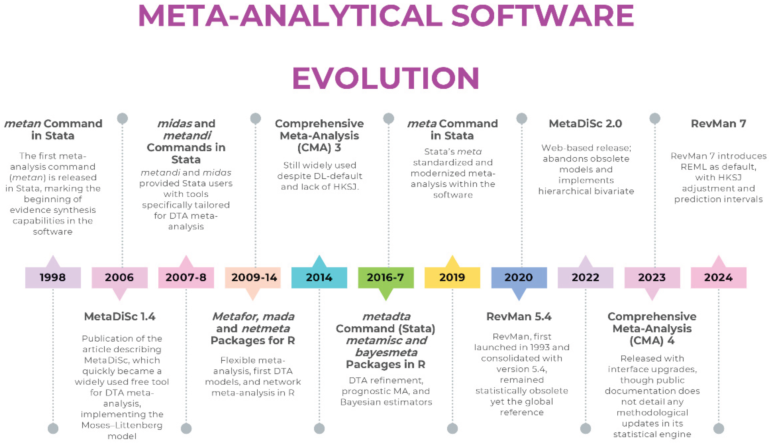
Figure 2.
Timeline of key methodological milestones in meta-analysis, illustrating the evolution from early heterogeneity estimators toward hierarchical and likelihood-based frameworks.
Figure 2.
Timeline of key methodological milestones in meta-analysis, illustrating the evolution from early heterogeneity estimators toward hierarchical and likelihood-based frameworks.
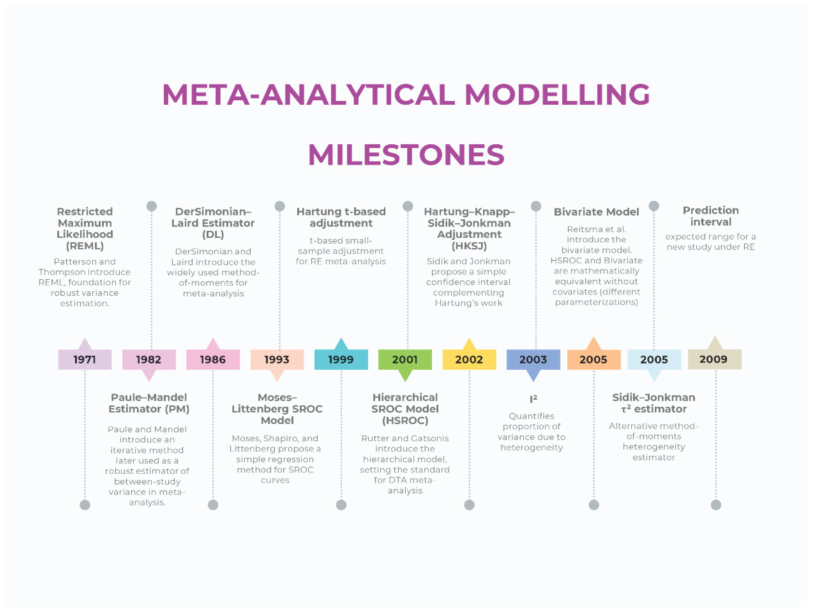

Table 1.
Overview of major meta-analysis software platforms, summarising their accessibility, available modelling features, and scope of implementation.
Table 1.
Overview of major meta-analysis software platforms, summarising their accessibility, available modelling features, and scope of implementation.
| Software | Domain focus | Main strengths (historical) | Major limitations | Status / maintenance | Adequacy |
|---|---|---|---|---|---|
| RevMan 5.4 | Interventions, DTA | Free, official Cochrane tool, intuitive interface | DL only, WT CIs, no PIs, DTA models, no advanced regression or Bayesian/network options | Replaced by RevMan 7 |  |
| RevMan 7 (Web) | Interventions, DTA | Successor to RevMan 5.4, updated interface, integration with Cochrane systems | DTA functionality limited to display of external parameters; Still limited compared to R/Stata in advanced modeling (e.g., lack of user-adjustable meta-regression or network meta-analysis) | Actively maintained |  |
| Meta-DiSc 1.4 | DTA | First free tool for diagnostic meta-analysis, simple interface | Separate Se/Sp, Moses–Littenberg only, no hierarchical modeling, no CIs/PIs | Still widely used because of historical citation patterns | |
| Meta-DiSc 2 | DTA | Modernized interface, implementation of hierarchical models | Lacks the advanced flexibility of script-based platforms (e.g., handling multiple covariates, non-linear models, or advanced influence diagnostics). Limited reproducibility compared to code-based solutions. | Released but limited adoption; partially solves 1.4 problems | |
| CMA 3 | Interventions | Affordable, easy GUI, widely adopted in early 2000s | Closed-code environment; estimation methods not directly inspectable, default DL, no HKSJ, limited estimators, no transparency or reproducibility | Commercial; not updated to current methods | |
| CMA 4 | Interventions | Affordable, easy GUI, implementation of PIs | Core model settings (e.g., estimator, CI method) remain undisclosed and presumably unchanged; problems of transparency and reproducibility persist | Commercial; not clarified if updated to current methods | |
| R (metafor, meta, mada) | Interventions, DTA, advanced | Full implementation of robust estimators, transparency, reproducibility, continuous updates | Statistical literacy and coding skills needed | Actively maintained |  |
| Stata (meta, metadta, midas, metandi) | Interventions, DTA | Robust, validated commands, widely used in applied research | Commercial license required, statistical literacy needed | Actively maintained | |
Legend: Robust and up to date (implements current recommended models and estimators); Restricted capabilities despite modern modelling (offers partial or limited implementation of current methods); Outdated/problematic (relies on obsolete estimators or defaults). DTA: Diagnostic Test Accuracy; GUI: Graphical User Interface; CMA: Comprehensive Meta-Analysis; HKSJ: Hartung–Knapp–Sidik–Jonkman; CI: Confidence Intervals; PI: Prediction Intervals; WT: Wald-Type; DL: DerSimonian–Laird; Se: Sensitivity; Sp: Specificity.
Robust and up to date (implements current recommended models and estimators); Restricted capabilities despite modern modelling (offers partial or limited implementation of current methods); Outdated/problematic (relies on obsolete estimators or defaults). DTA: Diagnostic Test Accuracy; GUI: Graphical User Interface; CMA: Comprehensive Meta-Analysis; HKSJ: Hartung–Knapp–Sidik–Jonkman; CI: Confidence Intervals; PI: Prediction Intervals; WT: Wald-Type; DL: DerSimonian–Laird; Se: Sensitivity; Sp: Specificity.
Table 2.
Common modelling behaviours associated with legacy software platforms and the corresponding methods that address these limitations within contemporary frameworks.
Table 2.
Common modelling behaviours associated with legacy software platforms and the corresponding methods that address these limitations within contemporary frameworks.
| Suboptimal modeling practice | Software | Why it is problematic | Solution / Recommended alternative |
|---|---|---|---|
| Random-effects with DL | RevMan 5.4, CMA | Underestimates τ² and produces narrower CIs when heterogeneity is present | Use REML or PM estimators (RevMan 7, R or Stata) |
| WT CIs with k > 2 and τ² > 0 | RevMan 5.4, CMA | Lower coverage when between-study variance is non-zero | Apply HKSJ or present both WT and HKSJ (RevMan 7, R or Stata) |
| No PI | RevMan 5.4, CMA | Does not describe dispersion of effects in new settings | Implement prediction intervals (RevMan 7, R or Stata) |
| Separate modeling of Se & Sp | MetaDiSc 1.4 | Does not account for correlation between Se & Sp | Use hierarchical models (Rutter & Gatsonis, Reitsma) (R or Stata) |
| Moses–Littenberg SROC | MetaDiSc 1.4 | Does not incorporate between-study variability | Use hierarchical models (Rutter & Gatsonis, Reitsma) (R or Stata) |
| No meta-regression with robust estimators | RevMan 5.4, MetaDiSc 1.4, CMA | Restricts ability to explore sources of heterogeneity | Use meta-regression (R or Stata) |
| Closed-code implementation | CMA | Internal algorithms not inspectable | Use script-based software (R or Stata) |
| Lack of advanced models (Bayesian, network, hierarchical) | All three | Cannot handle complexity of modern evidence synthesis | Use R (netmeta, bayesmeta) or Bayesian frameworks (JAGS, Stan) |
| Undeclared continuity correction (mHA) | RevMan 5.4, CMA (NS) | Imposes automatic corrections without disclosure | Use models handling zero cells directly (e.g., beta-binomial or Peto for rare events; in DTA, use bivariate/HSROC); alternatively, declare correction explicitly |
CMA: Comprehensive Meta-Analysis; CI: Confidence Interval; DL: DerSimonian–Laird; HSROC: Hierarchical Summary Receiver Operating Characteristic; HKSJ: Hartung–Knapp–Sidik–Jonkman; mHA: modified Haldane–Anscombe (0.5 continuity correction); NS: Not Specified; PI: Prediction Interval; PM: Paule–Mandel; REML: Restricted Maximum Likelihood; Se: Sensitivity; Sp: Specificity; SROC: Summary Receiver Operating Characteristic; WT: Wald-Type.
Table 3.
Practical guidance for selecting and reporting software and estimators in meta-analysis, with emphasis on alignment between modelling goals and implementation options.
Table 3.
Practical guidance for selecting and reporting software and estimators in meta-analysis, with emphasis on alignment between modelling goals and implementation options.
| For new meta-analyses, use platforms that allow explicit control of the estimator and uncertainty method rather than legacy versions such as RevMan 5.4, MetaDiSc 1.4, or CMA. |
| For intervention reviews: REML or PM estimators with HKSJ-adjusted CIs can improve uncertainty quantification; mHK may be useful when τ² is close to zero. |
| For DTA reviews: hierarchical bivariate (Reitsma) or HSROC (Rutter & Gatsonis) models provide joint estimation of Se and Sp. |
| Always report PIs in random-effects models. Reporting PIs enhances interpretability of random-effects estimates. |
| Favor transparent and reproducible solutions (R: metafor, meta, mada; Stata: meta, metadta, midas). |
| Report heterogeneity using the appropriate metrics (intervention: Q, I², τ²; DTA: τ²Se, τ²Sp, ρ), avoid univariate I² in DTA. |
| Explore heterogeneity properly through meta-regression and subgroup analyses. |
| When using methods that require continuity corrections for zero-cell studies (e.g., inverse-variance with ratio measures), the specific correction applied (e.g., mHA, Carter) should be reported so that the modelling step is transparent. Statistical models that handle zero cells directly—such as those based on the binomial likelihood (e.g., bivariate/HSROC models in DTA)—provide an alternative that does not require a continuity adjustment. |
CMA: Comprehensive Meta-Analysis; CI: Confidence Interval; HSROC: Hierarchical Summary Receiver Operating Characteristic; HKSJ: Hartung–Knapp–Sidik–Jonkman; mHK: modified Hartung–Knapp adjustment; mHA: modified Haldane–Anscombe (0.5 continuity correction); DTA: Diagnostic Test Accuracy; PI: Prediction Interval; PM: Paule–Mandel; REML: Restricted Maximum Likelihood; Se: Sensitivity; Sp: Specificity.
Disclaimer/Publisher’s Note: The statements, opinions and data contained in all publications are solely those of the individual author(s) and contributor(s) and not of MDPI and/or the editor(s). MDPI and/or the editor(s) disclaim responsibility for any injury to people or property resulting from any ideas, methods, instructions or products referred to in the content. |
© 2025 by the authors. Licensee MDPI, Basel, Switzerland. This article is an open access article distributed under the terms and conditions of the Creative Commons Attribution (CC BY) license (http://creativecommons.org/licenses/by/4.0/).
Copyright: This open access article is published under a Creative Commons CC BY 4.0 license, which permit the free download, distribution, and reuse, provided that the author and preprint are cited in any reuse.


