
Submitted:
20 October 2025
Posted:
22 October 2025
You are already at the latest version
Abstract
Decision Curve Analysis (DCA) bridges the gap between statistical accuracy and clinical usefulness—a distinction frequently overlooked in diagnostic research. Using a simulated cohort representing a real-world diagnostic scenario, this tutorial demonstrates how predictors with similar ROC-based performance can yield markedly different net benefit profiles when evaluated through DCA. Three tools were compared: a strong predictor (composite clinical score), a moderate biomarker (leukocytes), and a weak marker with modest AUC but limited practical value (serum sodium). Whereas ROC curves portray discrimination alone, decision curves situate performance within real clinical trade-offs, making explicit when a model adds value beyond default strategies such as treating all or none. The tutorial provides a step-by-step framework for interpretation, clarifies frequent misconceptions (thresholds, prevalence effects, calibration), and illustrates how DCA incorporates the consequences of decisions rather than just their statistical accuracy. Rather than adding ‘just another metric’, DCA reframes evaluation around a practical question: does using this model improve decisions across clinically reasonable thresholds?
Keywords:
decision curve analysis
; predictive models
; diagnostic accuracy
; calibration
; clinical utility
Main Text
In diagnostic and prognostic research, model performance is often assessed using traditional metrics such as sensitivity, specificity, and the area under the receiver operating characteristic curve (AUC). While these measures quantify discrimination—that is, a model’s ability to distinguish between patients who have a condition and those who do not—they provide limited insight into the clinical utility of a model—that is, whether using it leads to better decision-making in practice. However, AUC-based metrics remain blind to calibration and to the clinical consequences of false positives and false negatives. In other words, they answer whether the model ranks patients correctly, but not whether acting on its output leads to better decisions. DCA fills precisely this gap by quantifying whether using a model improves decisions across clinically relevant thresholds.
This limitation becomes particularly relevant in pediatrics, where decision thresholds—the level of risk at which a clinician decides to change their course of action (e.g., from observation to intervention)—may vary widely and interventions often carry age- or context-specific risks. A model may exhibit excellent statistical performance but still be unhelpful—or even harmful—if applied in an inappropriate context. Decision Curve Analysis (DCA) addresses this issue.
This manuscript introduces the core principles of DCA, illustrates its construction and interpretation, and demonstrates its application using simulated data from pediatric diagnostic research.
Fundamentals and Formula of Decision Curve Analysis
DCA is a method that estimates the net benefit of using a diagnostic or prognostic model at different threshold probabilities [1,2]. The net benefit is calculated as the number of true positives identified by a model, penalized by the number of false positives, and weighted by the relative harms of false-positive and false-negative decisions. This weighting represents the clinical trade-off between the harm of intervening unnecessarily (a false positive) and the harm of failing to intervene when needed (a false negative). This ratio arises directly from the theory of expected utility: at the threshold probability pt, the clinician is at the point of indifference where the expected harm of treating equals the expected harm of withholding treatment, and the odds term pt/(1−pt) is simply the mathematical expression of that indifference.
Net benefit is calculated as:
Net benefit = (TP/n) − (FP/n) × (pt / (1 − pt))
Where TP and FP are the number of true and false positives, n is the total sample size, and pt is the threshold probability—that is, the minimum level of predicted risk a clinician is willing to accept to justify a clinical intervention. Conceptually, is not merely a tolerated risk but the point of clinical indifference, where a clinician is equally willing to intervene or to withhold intervention because the expected harm of overtreatment equals the expected harm of undertreatment. This value captures the implicit balance between the harms of overtreatment and undertreatment. The clinical trade-off is then encoded mathematically in the final term of the equation, pt / (1 − pt), which serves as the penalty weight for each false positive. For example, a clinician might decide to operate only if a model predicts a risk of appendicitis of 20% or higher; in this case, pt = 0.20. This formula reflects the clinical trade-off between the benefits of identifying true positives and the harms of unnecessary treatment. For instance, if the threshold probability is set at 20%, the pt/(1−pt) ratio equals 0.25 (calculated as 0.20 / (1 − 0.20) = 0.25). In clinical terms, this means the model provides the equivalent of 25 additional correctly treated patients per 100, once false positives are penalized at pt/(1−pt). This means that each false positive is penalized as one-fourth of a false negative. In practical terms, it would take four unnecessary treatments (false positives) to cancel out the benefit of one correctly treated patient (true positive). This interpretation stems from the formula’s structure: the net benefit of one true positive can be considered as 1, while the penalty for one false positive is equal to the weight pt/(1-pt), which is 0.25 in this case. Therefore, the benefit of one true positive is canceled out by the cumulative harm of four false positives (since 4 × 0.25 = 1). This weighting directly reflects the clinician’s tolerance for overtreatment relative to undertreatment. It is important to clarify that in the DCA framework, ‘treatment’ refers to the clinical action taken based on the model’s output (e.g., performing surgery). The analysis thus assumes that a positive classification leads to this action, effectively equating overdiagnosis with overtreatment for decision-making purposes.
Suppose a threshold probability of 0.20 is chosen. This value is not arbitrary; it is the clinician’s explicit quantification of the balance between benefits and harms. Then pt / (1 − pt) = 0.25. If a model yields 60 true positives and 40 false positives in a sample of 200 patients, the net benefit would be:
Net benefit = (60/200) − (40/200 × 0.25) = 0.30 − 0.05 = 0.25.
This means the model provides the equivalent benefit of correctly treating 25 additional patients per 100 without unnecessary overtreatment.
The key idea behind DCA is to compare a model not just against chance, but against two clinically relevant extremes: treating all patients as positive or treating none. These two strategies can be evaluated using the same net benefit formula. For the ‘treat none’ strategy, no patients are treated, so both TP and FP are zero, resulting in a net benefit of 0 by definition. For the ‘treat all’ strategy, everyone is treated, meaning all patients with the condition are true positives and all patients without it are false positives. The formula adapts to this scenario, as will be shown later. In the context of a child presenting to the Emergency Department with abdominal pain and suspected acute appendicitis, these strategies would correspond to operating on every child regardless of further assessment (“treat all”) versus discharging all children without additional work-up or surgery (“treat none”). This provides a benchmark to assess whether a model adds value over existing clinical strategies. For instance, in our appendicitis example, a ‘treat all’ strategy would mean every child with abdominal pain undergoes surgery, leading to many unnecessary operations. A ‘treat none’ strategy would mean every child is sent home, potentially missing serious cases. A useful model must prove it provides more benefit than either of these simplistic—yet real-world—alternatives.
By plotting the net benefit of each strategy across a range of threshold probabilities, a decision curve graph is generated (see Figure 1 for examples). This graph shows whether and when a model provides higher clinical utility than blanket treatment or no treatment at all. A model with a higher net benefit across a relevant threshold range is considered more useful for decision-making.
Interpreting a Decision Curve
Returning to the previous example of suspected acute appendicitis in children, a decision curve can illustrate the clinical usefulness of a predictive model designed to guide surgical decision-making—that is, the decision to intervene. The “treat none” strategy assumes that no patient receives the intervention, and by definition its net benefit is always zero across all thresholds. The “treat all” strategy assumes every patient is treated, regardless of their predicted risk. Its net benefit depends on the prevalence of disease and declines as the threshold increases, since a higher threshold penalizes false positives more heavily. Formally, the net benefit of the “treat all” strategy can be expressed as:
Net benefit (treat all) = prevalence − (1 − prevalence) × (pt / (1 − pt))
In this equation, pt does not represent a threshold for the ‘treat all’ strategy itself (which has no threshold), but rather the clinician’s threshold against which this strategy is being evaluated. The decision curve plots the net benefit of ‘treat all’ across the entire range of possible clinician thresholds (pt on the x-axis) to serve as a benchmark. An immediate implication of this formulation is that as , the penalty term approaches zero and the net benefit of the “treat all” strategy converges to the disease prevalence. This is why, in every decision curve, the ‘treat all’ line intersects the y-axis at the prevalence—it represents the proportion of true positives obtained if everyone is treated in the absence of any false-positive penalty. A direct corollary is that the “treat all” curve crosses the x-axis (net benefit = 0) precisely when pt equals the disease prevalence: only clinicians whose treatment threshold lies below the baseline risk of the population would obtain net benefit from treating everyone.
This equation reflects the clinical trade-off of treating every patient—yielding true positives at the rate of disease prevalence, while incurring harm from unnecessary treatment of patients without the disease. As the threshold probability increases, the weight of false positives rises, leading to a progressive reduction in the net benefit of this strategy.
These two reference strategies serve as benchmarks for evaluating the added value of a predictive model.
The x-axis represents the threshold probability, which, as defined earlier, is the minimum predicted risk at which an intervention would be considered. The y-axis shows the net benefit, which combines true positives and false positives into a single metric weighted by the clinical consequences of misclassification.
Typically, three lines are plotted: one for the predictive model, one for the “treat all” strategy, and one for the “treat none” strategy. These serve as benchmarks against which the model’s added value can be judged. The model provides clinical benefit only in the range of thresholds where its curve lies above both reference strategies.
For example, if the model’s net benefit exceeds both “treat all” and “treat none” between 10% and 40% predicted risk, it suggests that its use is preferable to either universal or no intervention within that threshold range. Outside that range, the model may offer no advantage, and simpler decision rules may be equally or more effective.
Decision curves help determine whether, when, and to what extent a model is clinically useful—transforming statistical performance into actionable insight.
DCA and Prevalence
DCA is influenced by disease prevalence, since the balance between true positives and false positives depends on the frequency of the outcome in the population. In low-prevalence settings, the net benefit of treating all declines rapidly as the threshold increases, while in higher-prevalence settings, treating all may appear favorable over a broader range. Model-based curves are also shaped by prevalence, meaning that the same predictor can show different apparent utility depending on the baseline risk of the cohort. For this reason, decision curves should always be interpreted in light of the population context.
An Applied Example
To illustrate the application of decision curve analysis (DCA) in pediatric diagnostic research, a simulated dataset was constructed simulating a cohort of pediatric patients evaluated in the Emergency Department for abdominal pain with suspected acute appendicitis (Supplementary File 1). Before interpreting the decision curves, it is important to clarify that DCA is applied to the predicted probabilities generated by a fitted model, not to the raw predictor itself. The intermediate step is therefore the modeling process (typically logistic regression), which converts each predictor into an individualized probability of disease. The dataset comprised 200 simulated pediatric patients, with a prevalence of histologically confirmed appendicitis set at 20% and the remaining 80% representing non-specific abdominal pain. These prevalence values were chosen to approximate conditions in a typical Pediatric Emergency Department and are intended for illustrative purposes. A Pediatric Appendicitis Score (PAS) was calculated for each case. The score ranged from 0 to 10 and was calibrated to approximate performance reported in external validation, in line with Bhatt et al., where the AUC typically ranges from 0.80 to 0.90 [3]. Before applying DCA, each predictor must be converted into a risk prediction ranging from 0 to 1. For continuous predictors like leukocyte count or composite scores like PAS, this is typically achieved by fitting a logistic regression model with the predictor as the independent variable and appendicitis as the dependent variable. The fitted model generates a predicted probability of appendicitis for each patient based on their specific PAS or leukocyte value. These predicted probabilities are the quantities that are entered into the DCA equation, allowing the clinical utility of each predictor to be evaluated on the same decision-analytic scale.
As comparators, two continuous laboratory variables were included: total leukocyte count, representing a biomarker commonly used in the clinical diagnosis of acute appendicitis, and serum sodium, a marker reported to discriminate between complicated and uncomplicated appendicitis but without value for distinguishing appendicitis from non-surgical abdominal pain [4,5]. The simulated variables were generated to loosely mirror the real-world distribution of clinical findings in pediatric appendicitis, assuming independence between predictors. Each binary variable was assigned a prevalence consistent with existing literature. No correlation structures were imposed between predictors, reflecting a simplified yet educational design.
All statistical analyses were performed using Stata 19.0 (StataCorp LLC, College Station, TX, USA). Logistic regression models were fitted using the Pediatric Appendicitis Score (PAS), leukocyte count, and serum sodium as individual predictors. For each predictor, a binomial logistic regression model was used to generate individual predicted probabilities (), representing the estimated risk of appendicitis conditional on the observed predictor value. These predicted probabilities served as the input for Decision Curve Analysis, which evaluates the clinical utility of probabilistic predictions rather than raw predictor values. Discrimination was assessed through the area under the ROC curve (AUC) using 500 stratified bootstrap replications (stratified by outcome status) with percentile-based 95% confidence intervals (seed = 12345). The PAS showed excellent performance (AUC = 0.85; 95% CI: 0.79–0.91), leukocytes demonstrated moderate discrimination (AUC = 0.78; 95% CI: 0.70–0.86), and sodium performed poorly (AUC = 0.64; 95% CI: 0.55–0.73).
Calibration of all three models was assessed using the pmcalplot command (Supplementary File 2). Calibration plots demonstrated good concordance between predicted and observed probabilities for PAS and leukocyte count, whereas serum sodium exhibited systematic miscalibration across the risk spectrum. The Brier score—a metric that evaluates how well predicted risks match actual outcomes, where lower values indicate more accurate and clinically reliable predictions—further confirmed the hierarchy of performance: PAS achieved the lowest mean squared error (0.11), followed by leukocytes (0.13), while sodium performed worst (0.16). These results highlight the superiority of PAS, as it consistently provided the most accurate and clinically meaningful probability estimates.
Decision curve analysis with the dca package using a user-written Stata script based on Vickers et al.’s work [6] further highlighted the differences between these predictors (Figure 1). The PAS score demonstrated a consistent and clinically meaningful net benefit across a broad range of threshold probabilities, clearly outperforming both the “treat-all” and “treat-none” strategies, except at very high thresholds (>0.9), where the curve converged with “treat none” because the false-positive penalty term pt/(1–pt) diverges as pt→1. At that point, even a small number of false positives is sufficient to drive the model’s net benefit to ≈ 0, and the exact location of this convergence is primarily determined by prevalence rather than empirical model performance. The leukocyte count curve remained above both default strategies up to approximately 0.6, but then fell below “treat none.” This decline reflects the growing penalty for false positives at intermediate thresholds in the context of a 20% prevalence, which outweighs the modest number of true positives contributed by leukocytosis alone. A transient rise was observed between 0.7 and 0.9, driven by a small subgroup of patients with very high leukocyte counts who cross these extreme thresholds and temporarily improve net benefit. However, once the threshold approaches values where virtually no additional cases can be captured, the curve ultimately converges with “treat none.” By contrast, serum sodium did not separate meaningfully from the default strategies at almost any threshold, except for a brief interval between 0.2 and 0.3, underscoring its poor clinical utility despite an AUC in the modest discrimination range (≈0.65). This highlights a key lesson from DCA: a predictor can have statistically modest discrimination but still be clinically useless. These findings exemplify how ROC-based discrimination can overstate the clinical usefulness of weak predictors when assessed in isolation, whereas DCA provides a more direct evaluation of decision support. Calibration further complements this assessment. In the present example, sodium illustrates how a biomarker can underperform not only in discrimination but also in calibration, underscoring the need to evaluate all three dimensions when judging clinical applicability.
Two additional DCA analyses were then generated for the PAS score using simulated extreme prevalences within the same dataset, obtained via without-replacement stratified subsampling (i.e., retaining all cases from the majority class and randomly sampling from the minority class to achieve the target prevalence, rather than relabelling outcomes), while maintaining a comparable level of diagnostic performance (Figure 2). At a simulated prevalence of 5%, the decision curve showed broad overlap with the “treat none” strategy beyond a threshold probability of 0.5, reflecting the scarcity of true positive cases and the growing penalty of false positives as thresholds increase. Conversely, at a simulated prevalence of 70%, the curve demonstrated consistently high net benefit, exceeding both “treat all” and “treat none” strategies across the entire threshold range. This pattern is expected, as a high baseline risk increases the contribution of true positives and sustains net benefit even at more demanding thresholds.
This example illustrates how DCA can reveal significant differences in clinical utility between tools with similar ROC-based discrimination. A score that integrates multiple complementary predictors may offer substantially better decision support than a single biomarker, even when both achieve acceptable AUCs. In pediatric practice, this distinction can directly influence treatment decisions such as observation, imaging, or surgery.
As a final caveat, it should be emphasized that the discrimination, calibration, and decision curve results reported here reflect apparent performance, as they were obtained on the same simulated dataset used for model derivation. In real-world research, external validation or bootstrap correction would be required to avoid optimism and to ensure that the observed net benefit generalizes beyond the training sample
Strengths and Limitations of DCA
One of the main strengths of Decision Curve Analysis is its ability to incorporate clinical consequences into model evaluation directly [7,8,9]. Unlike formal decision-analytic models, which often require external estimates of utilities, costs or patient preferences, DCA can be applied directly to the validation dataset without the need for additional preference elicitation. It also handles continuous predictors natively, avoiding the discretization steps typically required in classical decision trees, which can distort performance or introduce artificial cut-points. These characteristics help explain why DCA offers a pragmatic alternative to more complex decision-analytic frameworks in routine model evaluation. This is achieved through the threshold probability (pt), which forces an explicit declaration of the harm-benefit trade-off. By evaluating a model across a range of these thresholds, DCA shows how its utility changes depending on different clinical perspectives on risk. Unlike traditional metrics such as AUC or accuracy—which measure statistical performance but ignore the decision context—DCA provides insight into whether a model leads to better outcomes by quantifying the trade-off between true positives and false positives. This makes it especially useful in scenarios with uncertain or variable decision thresholds, where the clinical value of a model depends not only on its discrimination but also on the harm-benefit balance of treatment decisions. DCA also allows models to be compared against real-world strategies such as treating all or none, offering a practical benchmark for clinical adoption.
While DCA is increasingly used in diagnostic research, it carries several interpretive limitations. First, its conclusions depend on the specification of threshold probabilities, which are inherently context-dependent and often subjective. Second, the method assumes a uniform misclassification cost across all patients—effectively encoding a single harm–benefit trade-off (pt) for the entire population. This assumption may be unrealistic in heterogeneous settings (e.g., a frail versus a low-risk patient may not incur equivalent harm from the same false positive). Third, DCA does not identify an ‘optimal’ threshold; it merely reports the net benefit if a given threshold is chosen. In practice, these constraints imply that DCA is best interpreted as a framework for comparative clinical utility rather than prescriptive decision-making, and may be complemented by tools such as decision impact curves. Nonetheless, DCA remains a uniquely intuitive tool for evaluating clinical utility in probabilistic terms. It is also important to emphasize, as highlighted by Kerr et al. [8], that the peak of a net benefit curve should not be interpreted as the ‘optimal’ clinical threshold. DCA is designed to show the relative net benefit across a range of thresholds, not to prescribe a single cut-off for decision-making
Special Considerations: Overfitting, Binary Predictors, and Calibration
One important methodological caveat in DCA is the risk of overfitting, particularly when the analysis is performed on the same dataset used for model derivation. This can lead to inflated estimates of net benefit that may not generalize to new data. Whenever possible, DCA should be conducted using external validation datasets or bootstrap-corrected predictions to avoid this bias.
Another common issue arises when DCA is applied to dichotomous predictors. Because such variables only generate a few distinct predicted probabilities (often just two), the resulting decision curve reduces to a single straight line segment, connecting the net benefit of the ‘treat none’ strategy to the net benefit observed at one point. This provides information over a much narrower range of thresholds compared with continuous predictors, restricting interpretability and limiting the assessment of clinical Utility.
Finally, DCA assumes that predicted probabilities are well-calibrated. If a model systematically over- or underestimates risk, the net benefit calculation will misrepresent its true clinical utility. Calibration can be evaluated using calibration plots, calibration slope and intercept, or the Brier score [9,10]. While calibration plots provide a visual assessment, the calibration slope and intercept offer quantitative measures of miscalibration. The Brier score aggregates prediction errors but can sometimes mask specific calibration deficiencies, so it should be interpreted alongside graphical methods. If calibration is poor, techniques such as logistic recalibration or shrinkage methods can help adjust predictions and improve decision-analytic performance [9,10].
An additional consideration, particularly relevant in pediatrics, is the small sample size often available. Limited data may lead to unstable estimates of net benefit, especially at extreme threshold probabilities. Simulation or bootstrap techniques may be required to assess variability in these contexts.
Conclusions
Decision Curve Analysis offers a powerful, clinically oriented framework for evaluating prediction models [7–9] (Figure 3). By directly quantifying net benefit across relevant thresholds, it clarifies whether, when, and how a model can improve decision-making. Combined with calibration, DCA complements traditional metrics by quantifying net benefit across relevant thresholds. In diagnostics—where both overtreatment and undertreatment carry distinct risks—this dual approach adds value beyond conventional metrics such as sensitivity, specificity, or AUC. For reliable application, however, DCA requires methodological rigor, including adjustment for overfitting and thoughtful handling of predictor types. Its systematic use in diagnostic research can better align statistical evaluation with real-world clinical benefit.
Funding
None declared.
Institutional Review Board Statement
Not Applicable.
Informed Consent Statement
Not Applicable.
Data Availability Statement
The dataset used in this study is simulated and has been provided as supplementary material (Supplementary File 1).
Conflicts of Interest
The author states no conflict of interest.
Use of Artificial Intelligence
Artificial intelligence (ChatGPT 4, OpenAI) was used for language editing and for generating a simulated dataset under the author’s explicit instructions. It did not influence the scientific content, analysis, or interpretation.
References
- Vickers AJ, Elkin EB. Decision curve analysis: a novel method for evaluating prediction models. Med Decis Making. 2006, 26, 565–74. [Google Scholar] [CrossRef] [PubMed] [PubMed Central]
- Vickers A J, Van Calster B, Steyerberg E W. Net benefit approaches to the evaluation of prediction models, molecular markers, and diagnostic tests BMJ 2016, 352, i6. [CrossRef]
- Bhatt M, Joseph L, Ducharme FM, Dougherty G, McGillivray D. Prospective validation of the pediatric appendicitis score in a Canadian pediatric emergency department. Acad Emerg Med. 2009, 16, 591–6. [Google Scholar] [CrossRef] [PubMed]
- Kottakis G, Bekiaridou K, Roupakias S, Pavlides O, Gogoulis I, Kosteletos S, Dionysis TN, Marantos A, Kambouri K. The Role of Hyponatremia in Identifying Complicated Cases of Acute Appendicitis in the Pediatric Population. Diagnostics (Basel) 2025, 15, 1384. [Google Scholar] [CrossRef] [PubMed] [PubMed Central]
- Duman L, Karaibrahimoğlu A, Büyükyavuz Bİ, Savaş MÇ. Diagnostic Value of Monocyte-to-Lymphocyte Ratio Against Other Biomarkers in Children With Appendicitis. Pediatr Emerg Care. 2022, 38, e739–e742. [Google Scholar] [CrossRef] [PubMed]
- Vickers AJ, Cronin AM, Elkin EB, Gonen M. Extensions to decision curve analysis, a novel method for evaluating diagnostic tests, prediction models and molecular markers. BMC Med Inform Decis Mak. 2008, 8, 53. [Google Scholar] [CrossRef] [PubMed] [PubMed Central]
- Van Calster B, Wynants L, Verbeek JFM, Verbakel JY, Christodoulou E, Vickers AJ, Roobol MJ, Steyerberg EW. Reporting and Interpreting Decision Curve Analysis: A Guide for Investigators. Eur Urol. 2018, 74, 796–804. [Google Scholar] [CrossRef] [PubMed] [PubMed Central]
- Kerr KF, Brown MD, Zhu K, Janes H. Assessing the Clinical Impact of Risk Prediction Models With Decision Curves: Guidance for Correct Interpretation and Appropriate Use. J Clin Oncol. 2016, 34, 2534–40. [Google Scholar] [CrossRef] [PubMed] [PubMed Central]
- Steyerberg EW, Vickers AJ, Cook NR, Gerds T, Gonen M, Obuchowski N, Pencina MJ, Kattan MW. Assessing the performance of prediction models: a framework for traditional and novel measures. Epidemiology. 2010, 21, 128–38. [Google Scholar] [CrossRef] [PubMed] [PubMed Central]
- Steyerberg, E.W. (2019). Clinical Prediction Models: A Practical Approach to Development, Validation, and Updating (2nd ed.). Springer.
Figure 1.
Receiver operating characteristic (ROC, upper panels) and decision curve analysis (DCA, lower panels) for three predictors of acute appendicitis in a simulated pediatric emergency cohort (n=200, prevalence 20%). The left panels display results for serum sodium, which achieved only modest discrimination (AUC 0.64; 95% CI: 0.55–0.73). Its DCA curve largely overlapped with the “treat-none” and “treat-all” strategies across thresholds, with only a minimal interval of apparent net benefit around 0.2–0.3, underscoring its lack of practical utility despite AUC values commonly reported in the literature. The middle panels correspond to total leukocyte count, which demonstrated moderate discrimination (AUC 0.78; 95% CI: 0.70–0.86). Its decision curve remained above both default strategies up to ~0.6, then declined below “treat none” as false-positive penalties outweighed the modest number of true positives. A transient rise was observed between thresholds of 0.7 and 0.9, reflecting the contribution of a small subgroup with markedly elevated leukocyte counts, before ultimately converging with “treat none” at extreme thresholds. The right panels show the Pediatric Appendicitis Score (PAS), which was calibrated to mirror external validation studies and yielded good overall discrimination (AUC 0.85; 95% CI: 0.79–0.91). In DCA, PAS consistently provided greater net benefit than either “treat-all” or “treat-none” across almost the entire range of thresholds, except beyond 0.9, where convergence with “treat none” occurred as expected given the simulated prevalence. Accordingly, the figure should be interpreted as supporting model choice within clinically relevant thresholds. Collectively, these analyses highlight how ROC-based discrimination can overestimate the clinical value of weaker predictors, while DCA offers a more direct appraisal of their decision-making utility.
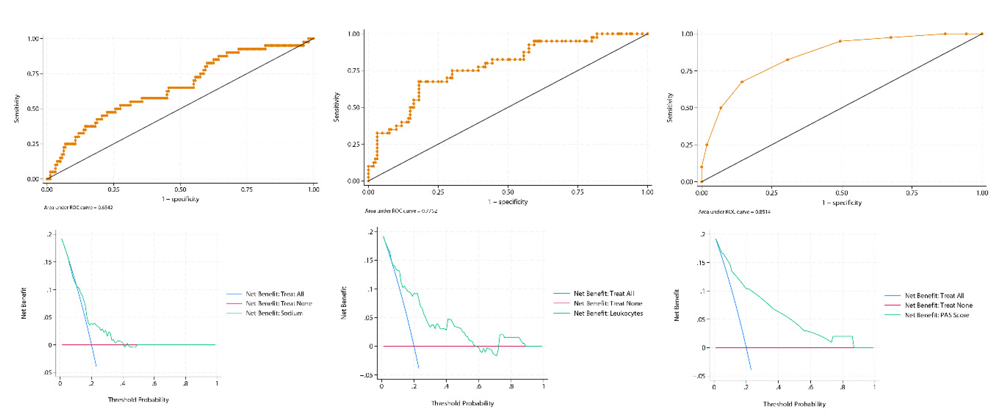
Figure 2.
Decision curve analysis of the Pediatric Appendicitis Score (PAS) under simulated extreme prevalence scenarios. Prevalence scenarios of 5% and 70% were generated by stratified random subsampling of the original dataset. For each subset, the PAS model was refitted and predicted probabilities were recalculated before performing DCA. At a prevalence of 5%, the curve overlaps substantially with the “treat none” strategy beyond a threshold probability of 0.5, illustrating the limited contribution of true positives and the increasing penalty of false positives in a low-prevalence setting. At a prevalence of 70%, the curve shows consistently high net benefit, remaining above both “treat all” and “treat none” across the full range of thresholds, as expected when baseline risk is high and true positives predominate.
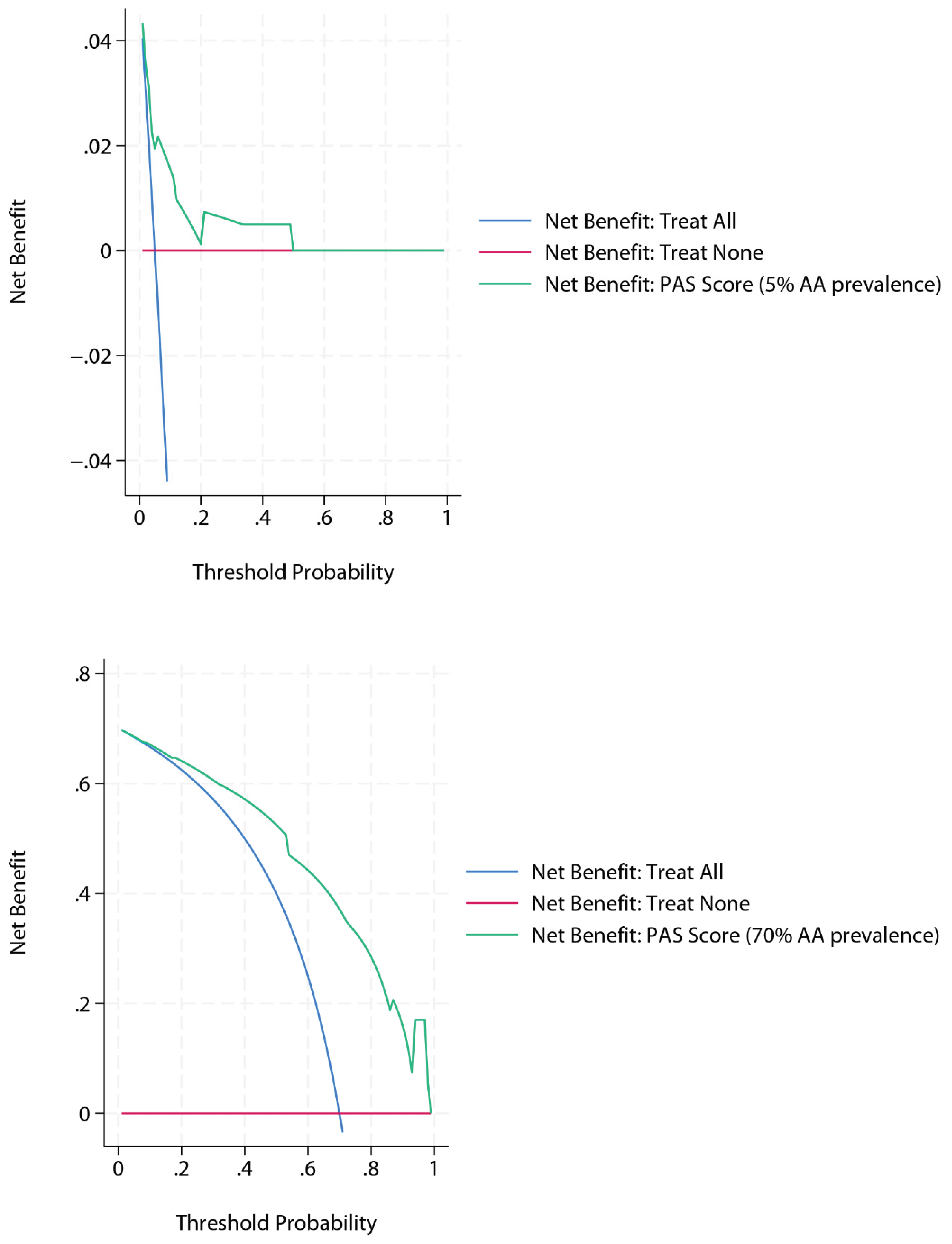
Figure 3.
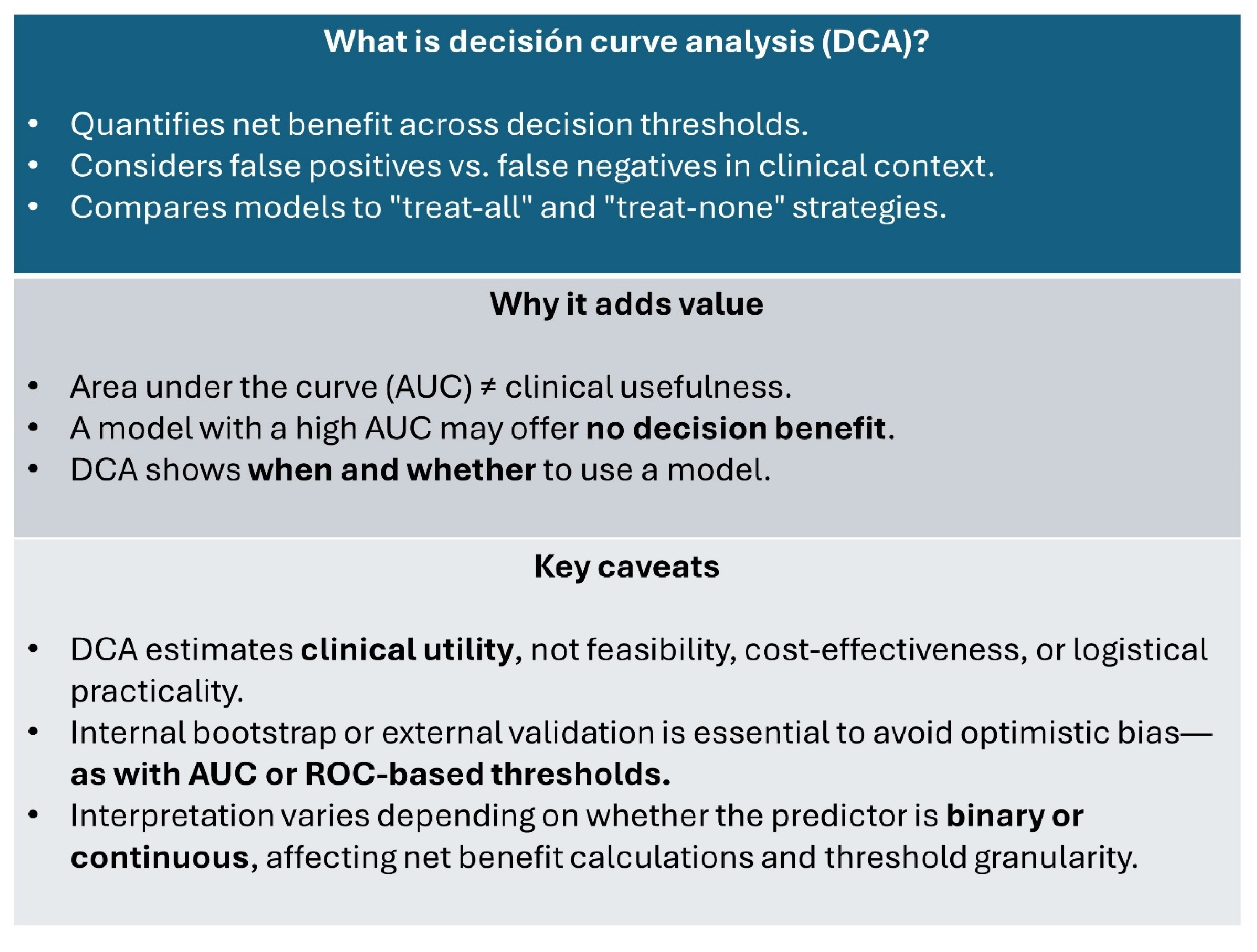
Summary of the core principles of Decision Curve Analysis (DCA). This visual overview outlines what DCA is, how it adds value beyond traditional performance metrics like AUC, and key interpretive caveats. It highlights DCA’s focus on clinical utility—quantifying net benefit across decision thresholds—and its ability to compare models against “treat-all” and “treat-none” strategies. Unlike AUC, DCA shows whether and when a model improves decision-making. However, its interpretation depends on correct threshold specification, external validation, and the nature of the predictor (binary vs. continuous).
Figure 3.
Summary of the core principles of Decision Curve Analysis (DCA). This visual overview outlines what DCA is, how it adds value beyond traditional performance metrics like AUC, and key interpretive caveats. It highlights DCA’s focus on clinical utility—quantifying net benefit across decision thresholds—and its ability to compare models against “treat-all” and “treat-none” strategies. Unlike AUC, DCA shows whether and when a model improves decision-making. However, its interpretation depends on correct threshold specification, external validation, and the nature of the predictor (binary vs. continuous).
Disclaimer/Publisher’s Note: The statements, opinions and data contained in all publications are solely those of the individual author(s) and contributor(s) and not of MDPI and/or the editor(s). MDPI and/or the editor(s) disclaim responsibility for any injury to people or property resulting from any ideas, methods, instructions or products referred to in the content. |
© 2025 by the authors. Licensee MDPI, Basel, Switzerland. This article is an open access article distributed under the terms and conditions of the Creative Commons Attribution (CC BY) license (http://creativecommons.org/licenses/by/4.0/).
Copyright: This open access article is published under a Creative Commons CC BY 4.0 license, which permit the free download, distribution, and reuse, provided that the author and preprint are cited in any reuse.


