Clinical Prediction Models: Foundational Concepts

Javier Arredondo Montero

doi:10.20944/preprints202510.1981.v1

Submitted:

25 October 2025

Posted:

27 October 2025

You are already at the latest version

Abstract

Background: Clinical prediction requires formalizing uncertainty into a statistical model. However, persistent confusion between prediction and inference, and between traditional (stepwise) and modern (penalized) development strategies, leads to unstable, poorly calibrated, and overfit models. A structured statistical framework is essential. Methods: This article is a structured, didactic tutorial that explains the core concepts of clinical prediction. It covers the definition of a prediction model, the fundamental strategies for its construction, and the essential framework for its evaluation. Results: The tutorial demystifies model construction by contrasting robust modern methods (penalized regression, LASSO) against traditional approaches (univariable filtering, stepwise selection). It explains how to manage key pitfalls such as collinearity (VIF), non-linearity (RCS), and interaction terms. Finally, it provides a comprehensive assessment framework by reframing model performance into its three essential domains: discrimination (ranking ability), calibration (probabilistic honesty), and validation (generalizability). Conclusions: This guide provides clinicians with the essential methodological foundation to critically appraise and understand modern prediction models.

Keywords:

clinical prediction models

;

logistic regression

;

LASSO

;

overfitting

;

variable selection

;

calibration

;

validation

;

stepwise

;

tutorial

;

guide

Subject:

Medicine and Pharmacology - Clinical Medicine

Formalizing the 'Clinical Gestalt': A Conceptual Introduction to Prediction

Clinical decision-making is fundamentally the management of uncertainty. Clinicians constantly process multiple data sources—history, examination, labs, and imaging—and mentally prioritize the few truly informative features. In statistical terms, these are the predictors: structured information used to estimate the likelihood of a clearly defined outcome.

Senior clinicians develop an internal “algorithm” through experience: they weigh certain findings more heavily than others and combine them into a probability judgment. A statistical model formalizes this same reasoning process. It is an explicit mathematical equation assigning a coefficient (weight) to each predictor, functioning as the engine that transforms clinical inputs into a risk estimate.

This transformation produces a quantitative prediction—not merely “high suspicion,” but an individualized probability (e.g., 75%) for a specific patient. A predictive model is therefore a structured and testable version of the clinician’s gestalt: a reproducible mechanism that answers a single question — “Given this patient’s profile, what is their personal risk of the outcome?” [1]

The Model's Purpose: Prediction vs. Inference

Now that we have defined our model as an "engine," we must ask what its fundamental purpose is. A model's engine can be built to do two very different jobs [2]:

Job #1: The "Why" Job (Finding the Most Valuable Player)

Sometimes the goal is not to forecast an outcome, but to understand which factor matters most. Here we "isolate the MVP": the question is whether one variable remains independently associated with the outcome after accounting for the others.

Key Question: "Is this one specific factor truly and independently linked to the outcome?"
Goal: To test a single factor’s isolated importance (e.g., “Is a high WBC count strongly linked to perforated appendix on its own?”).
Method: Build a model that adjusts for other variables (like age or symptom duration) to isolate that association.
Limitation: It identifies importance but not predictive usefulness; a factor may be biologically relevant yet contribute little to individual risk estimation.

Job #2: The "What" Job (Predicting the Game)

A different task: instead of explaining why, we estimate "What is this patient's probability?"
Key Question: “What is this specific patient’s personal risk of the outcome?”
Goal: Generate the most accurate forecast, not a causal explanation.
Method: Use all variables that improve prediction — including those not independently associated — just as a “home advantage” predicts the score without reflecting player skill.

Why This Distinction Is Everything

An associated factor may be a poor predictor (a star player who is injured today), while a non-causal factor may be highly predictive (home field advantage). In clinical terms, WBC count is associated with perforation (Job 1), but duration of symptoms >48 hours may better forecast this child’s risk (Job 2).

This guide is concerned exclusively with Job #2: Prediction — building and evaluating models designed to generate accurate patient-level forecasts. Now that we have established our goal is exclusively prediction (Job #2), we must examine the statistical "engine" that allows us to build that forecast.

The Engine of Prediction: A Look Inside

We have defined our predictive model as an "engine" that takes in predictors and outputs a probability. Now, we must look at the mechanics of that engine.

The "Yes/No" Problem

Most clinical outcomes are binary — the diagnosis is present or absent, the patient does or does not develop a complication, or survives or dies. We are not estimating “how much,” but simply whether the event occurs (Yes/No). Examples include:

Diagnosis: Does this patient with right lower quadrant pain actually have appendicitis? (Yes/No)
Morbidity: Will this patient develop a surgical site infection? (Yes/No)
Mortality: Will this specific patient die within 30 days of surgery? (Yes/No)

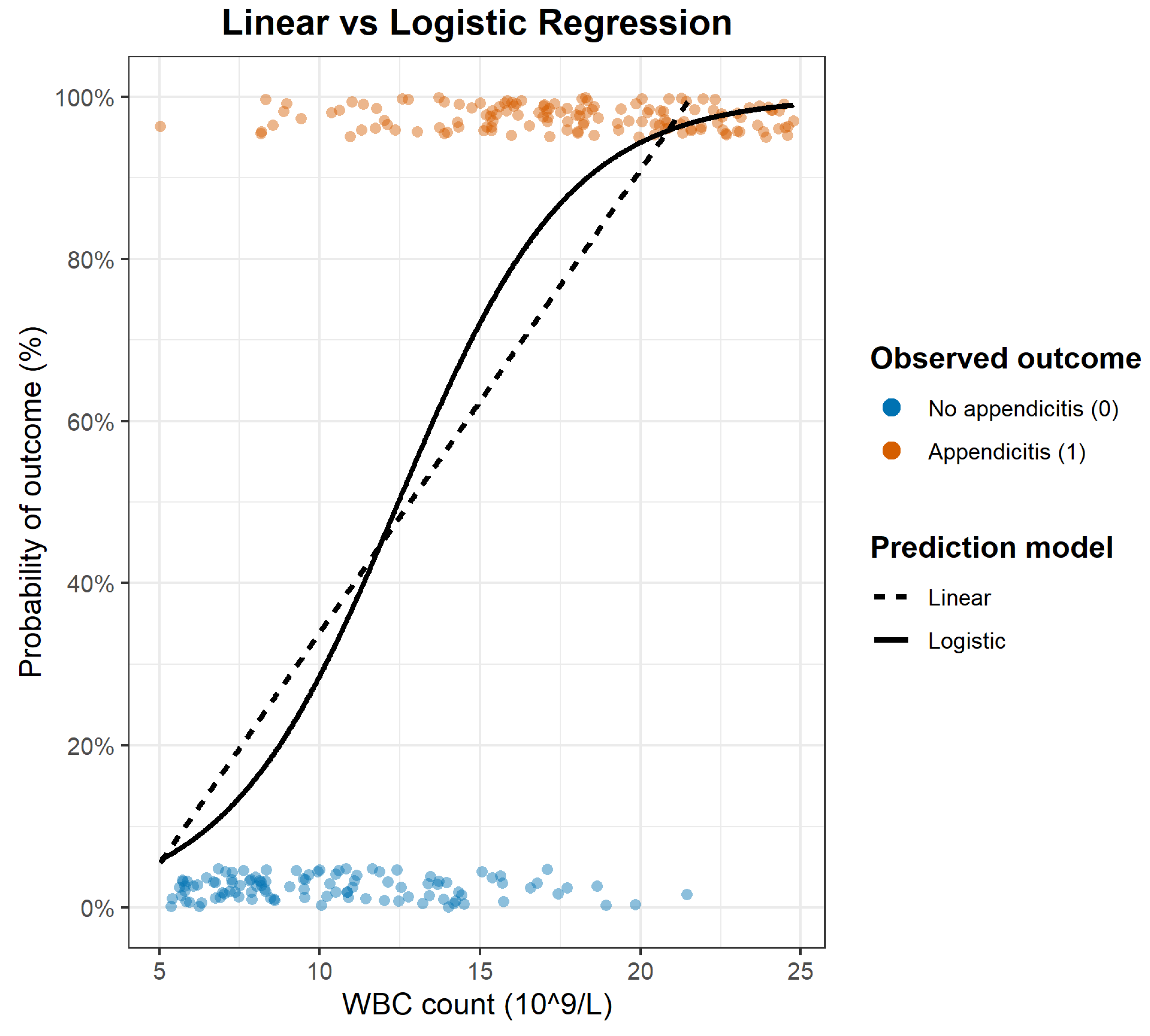
The Foundational Tool: Linear Regression

Regression is the formal process of linking predictors (inputs) to an outcome (output). Linear regression is the simplest version: it fits a straight line describing how a predictor relates to a continuous outcome (e.g., Age vs. Blood Pressure) [3]. However, because this line is unbounded, applying it to binary outcomes produces mathematically impossible results (e.g., −20% or 180% probability), making it unsuitable for prediction in most clinical tasks.

Logistic Regression: The Standard Model for Binary Outcomes

To solve this, we need a bounded engine — logistic regression [3,4]. Instead of a straight line, it applies the logistic function, generating a characteristic S-shaped (“sigmoid”) curve (Figure 1) that asymptotically approaches 0% and 100% and never exceeds those limits. When fitting the model, the engine learns two intuitive features:

Center (Location): where predicted probability crosses ~50% — the tipping point along the predictor scale.
Steepness (Slope): how sharply risk changes near that point — a steep slope signals a strong predictor, a flat one a weak effect.

Logistic regression is a powerful and intuitive foundation, but it is only one model among many. Predictive modeling is a broad field with numerous alternative “engines.” This tutorial focuses on logistic regression because it is widely used and clinically interpretable, but it also has limitations: it assumes a linear predictor-risk relationship, performs poorly with very high-dimensional data, and cannot naturally model complex non-linearity or interactions. Modern extensions — such as penalized regression — were developed specifically to address these limitations. The dual focus of this guide is therefore pragmatic: clinicians must first understand the classical foundation before extending it with modern tools that improve realism, parsimony, and stability.

The Multivariable Challenge: From a Simple Tool to a Real-World Model

While a single-predictor model is useful for illustration, real patients require integrating multiple pieces of information. Risk depends not only on WBC count but also imaging, symptom duration, and other clinical features. Multivariable models must combine these inputs while handling their interrelationships. This introduces three major challenges: collinearity, overfitting, and variable selection — issues we now address.

The Limits of a Single Predictor

A one-variable model is didactic but unrealistic. In actual clinical reasoning, a senior clinician never relies on a single piece of data but implicitly combines several predictors (e.g., WBC, age, symptom duration) to form a probability judgment.

This brings us to the next challenge: how does a model handle multiple predictors simultaneously?

The Multivariable Logistic Regression Engine

A multivariable logistic regression model works through the same two-step mechanism:

Step 1 – Linear Predictor (Score): All predictors are combined into a single number by multiplying each by its coefficient and summing the results — a mathematical translation of the clinical gestalt. This produces an “unbounded” score, just like in linear regression.
Step 2 – Logistic Transformation (Probability): That score is then passed through the logistic (S-shaped) function, which converts it into a valid probability between 0% and 100%.

Modeling Complexity: Non-linearity and Interactions

Standard logistic regression assumes a linear relationship between predictor and risk — that risk rises at a constant rate. Real clinical data rarely behave this way. For example, postoperative risk might remain stable from ages 20–60 and increase sharply only beyond that threshold. If this non-linearity is ignored, the model systematically over- or under-predicts at the extremes, harming calibration.

Restricted Cubic Splines (RCS)

The standard approach for handling non-linear continuous predictors is Restricted Cubic Splines (RCS) [5,6]. Unlike a straight-line assumption, RCS allows the model to follow the actual risk curve observed in the data. The predictor’s range is partitioned using predefined “knots” (often fixed quantiles such as the 10th, 50th, and 90th percentiles), and smooth polynomial segments are fitted between them. This lets the slope change where clinically meaningful changes in risk occur, rather than enforcing a single uniform effect.

This flexibility comes at a cost in degrees of freedom, so knot placement must be economical. In practice, using 3–5 knots captures clinically relevant curvature while avoiding overfitting. RCS therefore improves calibration by aligning the functional form of the predictor with its true biological behavior, instead of forcing it into a misleading linear approximation.

Critical Pitfalls in Predictive Modelling

While the two-step modeling process looks simple, the real difficulty lies in how the model learns the coefficients for multiple predictors. When many variables are included (10, 50, 100+), several methodological threats emerge.

The Problem of Collinearity (Redundant Predictors): Collinearity occurs when predictors provide overlapping information — effectively “echoing” each other [7]. For example, WBC count and Absolute Neutrophil Count describe the same biological process and tend to move together. This makes the model unstable because it cannot determine how to apportion the weight between them. The result can be extreme or contradictory coefficient estimates. Collinearity is diagnosed using the Variance Inflation Factor (VIF): a VIF of 1 indicates independence, while higher values (often >5 or >10) signal inflated variance and coefficient instability [7].
The Problem of "Noise" vs. "Signal" (Overfitting): Clinical reasoning is naturally parsimonious: it prioritizes a few strong predictors and ignores irrelevant noise [6]. Overfitting occurs when a model does the opposite — including too many weak or irrelevant variables for the available sample size. The Events Per Variable (EPV) ratio is a key indicator of this risk. The traditional rule of thumb is 10 EPV [8], but modern studies show this threshold is not universal: the required EPV depends on predictor strength and modeling strategy. Penalized methods like LASSO can safely operate with lower EPV because they constrain complexity, whereas even 10 EPV may be inadequate when predictors are weak. When EPV is too low, the model starts “memorizing” random quirks in the data rather than learning real patterns — classic overfitting. This leads to unstable coefficients and poor performance on new patients, a finding confirmed repeatedly by simulation studies [9]. The dataset used in Figure 2 illustrates the opposite case: high EPV ensures stability.
The Challenge of Missing Data: Missingness is widespread in clinical datasets and can introduce bias if poorly handled [10]. Common but flawed approaches include complete-case analysis (dropping patients with any missing value, reducing power and distorting representativeness) and mean imputation (which falsely shrinks variability). The recommended approach for data that are Missing At Random is Multiple Imputation (MI) [11], which creates several plausible datasets and pools their estimates, yielding unbiased coefficients and correctly estimated uncertainty.

This leads to the central challenge of model development: selecting the small group of true signal predictors and discarding the noise — the core problem of variable selection.

Figure 2. This example uses a different simulated dataset for purely didactic purposes to demonstrate the fundamental principle of the Least Absolute Shrinkage and Selection Operator (LASSO) for building robust predictive models, using a model to predict the binary outcome of appendicitis (yes/no) from four predictors. The horizontal axis represents the penalty strength (log λ): as we move from left to right, the penalty increases, forcing the model to become simpler and more parsimonious. The vertical axis shows the magnitude of the coefficient (β) assigned to each predictor — that is, its predictive contribution to the model (higher absolute values indicate a stronger predictive effect). The horizontal line at zero marks the point at which a variable is effectively removed from the model. In this example, LASSO demonstrates four key actions: first, the Appendix Diameter by Ultrasound (green line) is the most dominant predictor, is the least penalised, and is the last to be shrunk toward zero (dominant predictor). Second, WBC Count (blue line) is a strong predictor that remains active until higher penalty levels (strong predictor). Third, LASSO efficiently resolves the collinearity between the strong White Blood Count (WBC) and the redundant ANC (Absolute Neutrophil Count) (orange dashed line), which is eliminated earlier because it adds overlapping information (redundant predictor). Fourth, Age (grey dotted line) behaves as weak noise, with a small negative coefficient that is rapidly reduced to zero (weak/noise predictor). The dotted vertical lines indicate two common choices for the optimal penalty (λ) identified through cross-validation. λₘᵢₙ represents the penalty that results in the model with the lowest mean cross-validated error—the most accurate model on average. However, the "one-standard-error rule" favors parsimony and selects λ₁ₛₑ. This rule identifies the simplest model (i.e., the one with the highest penalty) whose performance is statistically indistinguishable from the best model (within one standard error of the minimum error). At λₘᵢₙ, the weak 'Age' predictor is still included. By moving to λ₁SE, we accept a marginal, statistically non-significant decrease in performance in exchange for a more robust and simpler model that has correctly shrunk the coefficients for both the weak ('Age') and redundant ('Neutrophil Count') predictors to zero, retaining only the strongest signals.

Building the Model: The Challenge of Variable Selection

Variable selection determines which predictors are retained in the final model — the key decision in Step 1 of model building. When many candidate predictors are available, choosing the few true “signal” variables while excluding “noise” is essential to avoid instability. The methods used for this selection differ widely in statistical validity, which is why we now contrast classical approaches with modern penalized solutions. Table 1 shows the inclusion criteria, downstream effects on the final model, and methodological status of common variable selection methods, contrasting univariable filtering and stepwise with LASSO.

Let's explore the common approaches, from the classical to the modern.

The Classical "Manual" Method: Univariable Filtering

This is an intuitive, two-step manual approach that many researchers have used.

Step 1 (Filter): Run separate univariable regressions for each candidate predictor (e.g., 100 variables, as an illustrative example).
Step 2 (Build): From the results, keep only predictors with a “promising” p-value (e.g., p < 0.10–0.20), rank them by Odds Ratio or coefficient size, and select a fixed number of “top” variables (e.g., 5–10) for the final multivariable model.

Although seemingly logical, this approach is methodologically weak. A variable that appears nonsignificant alone may become highly predictive once adjusted for others (e.g., “Fever” becomes powerful when combined with “Symptom Duration”). The method therefore risks discarding useful predictors and does nothing to resolve collinearity.

The "Automated" Method: Stepwise Regression

Stepwise regression was introduced as an automated alternative to manual filtering [9]. It selects variables based on p-values using two variants:

Forward stepwise: start with no variables and keep adding the “most significant” ones until none meet the entry threshold.
Backward stepwise: start with all candidate predictors and remove the least significant until all remaining satisfy the retention threshold.

This "hands-off" approach appears objective, but the selection rules (the “p-to-enter” and “p-to-remove” thresholds) are arbitrary, which is why stepwise is now recognized as statistically flawed. In practice, it becomes a p-value hunting machine: it captures spurious correlations, amplifies noise, and is structurally designed to overfit.

It is also highly unstable. If stepwise is run on two slightly different samples from the same population, it often selects different predictors, yielding two entirely different “final” models — a clear sign of lack of reproducibility.

Even its apparent advantage in handling collinearity is misleading. Although the algorithm will drop one of two correlated variables, the choice depends solely on which has the slightly better p-value at that moment. With tiny shifts in the data, the preference can flip (e.g., WBC p=0.001 vs ANC p=0.002), causing the opposite variable to be retained. The result is an unstable model driven by chance rather than statistical robustness.

In short, stepwise regression frequently produces fragile, non-generalizable models and is strongly discouraged in predictive modeling [9]. Classical regression texts describe these limitations extensively and show why ordinary least-squares approaches fail in high-dimensional or non-linear settings [12].

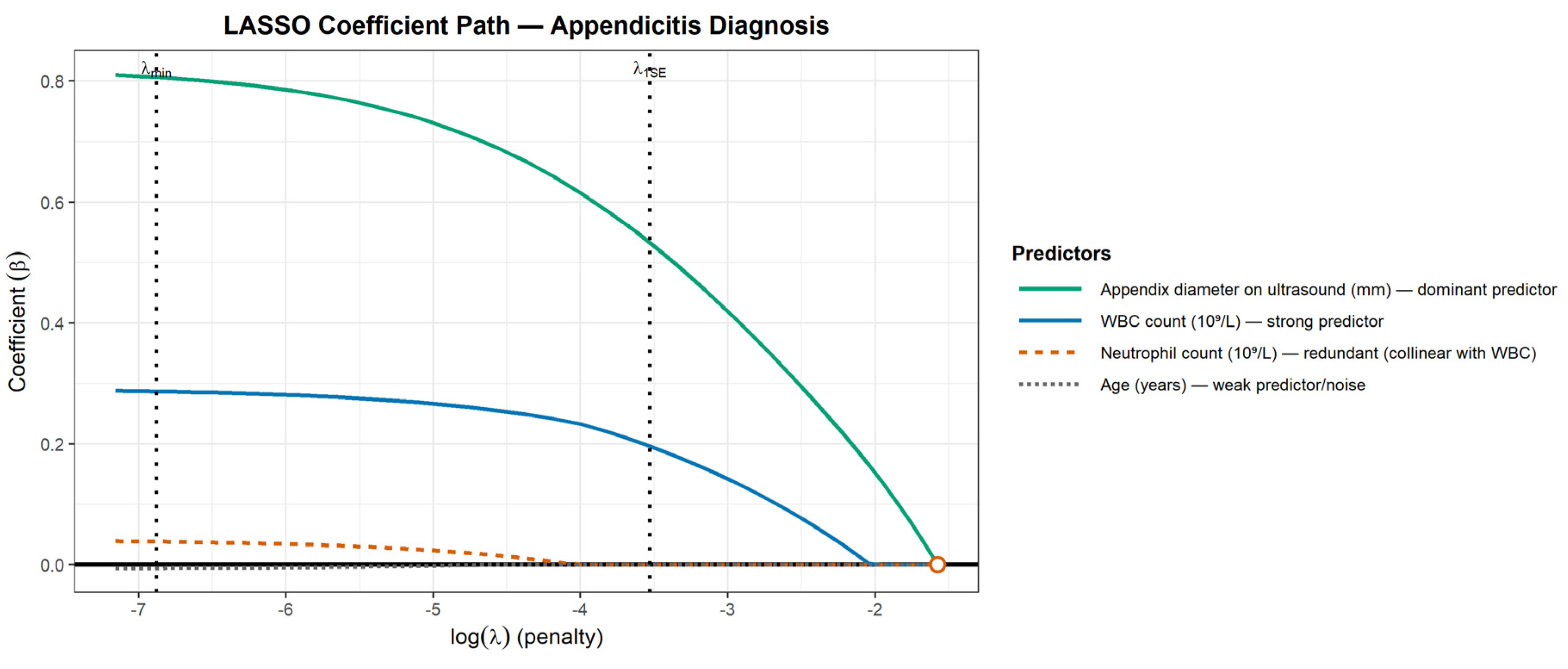
The Modern Solution: LASSO (Least Absolute Shrinkage and Selection Operator) Regression

LASSO is the most widely adopted modern alternative to classical variable selection because it directly targets the two major failures of univariable filtering and stepwise: overfitting and collinearity [13]. Unlike stepwise, which adds or removes variables based on unstable p-values, LASSO begins with all candidate predictors and applies a penalty that discourages unnecessary complexity. This penalty enforces parsimony in the same way an experienced clinician ignores “background noise” and keeps only the information that actually changes the prediction.

The strength of this penalty is governed by λ (lambda):

small λ → minimal shrinkage → more variables retained
large λ → stronger shrinkage → weak predictors forced toward zero

Critically, the optimal λ is not chosen arbitrarily. It is selected via k-fold cross-validation, meaning it is tuned using out-of-sample performance rather than p-values or convenience rules. This makes the method data-driven and far more stable than stepwise.

As λ increases, LASSO gradually shrinks small or redundant coefficients until many become exactly zero, at which point those variables are effectively removed from the model. That is why LASSO performs variable selection and model fitting simultaneously, instead of separating those steps like older methods.

This produces three major advantages:

Prevents overfitting by penalizing unnecessary complexity.
Handles collinearity naturally — between two redundant predictors, one is retained and the other is suppressed.
Improves reproducibility because the selection is based on penalized optimization rather than fragile p-value thresholds.

In short, LASSO does what clinicians intuitively do: it keeps what matters, removes what does not, and does so in a principled, mathematically controlled way — without the instability of stepwise.

LASSO belongs to a broader family of penalized (regularized) methods. Ridge regression is a related approach that also shrinks coefficients but typically does not reduce them to exactly zero, meaning all variables remain in the model with reduced influence. Elastic Net combines both LASSO and Ridge: it can shrink coefficients and retain correlated predictors as a group, which is advantageous when strong collinearity exists (e.g., WBC vs ANC).

Thus, penalized regression is not a single method but a framework. LASSO is preferred when parsimony is the priority; Elastic Net is favored when preserving correlated clinical signals is important; Ridge is useful when stabilization matters more than variable elimination. These represent modern, statistically valid alternatives to classical selection methods and form the foundation for the next stage: evaluating the resulting model’s quality across discrimination, calibration, robustness, and clinical utility.

Table 2 presents the four complementary quality domains—discrimination, calibration, robustness (internal validation), and clinical utility—along with typical metrics and their functional interpretations.

Model Assessment: Validation and Calibration

Breaking Down the Jargon: The ROC Curve

The Receiver Operating Characteristic (ROC) curve is the most widely cited measure of model performance in clinical literature, and because of this ubiquity it is often mistakenly treated as a form of validation. In reality, ROC analysis is a descriptive tool, not a validation method; it summarizes how the existing logistic regression model performs in terms of discrimination [14,15].

Model Linkage: The ROC curve is created by plotting sensitivity against specificity across every possible probability threshold generated by the logistic model. The model is the engine; the ROC simply visualizes how well it separates those with and without the outcome.
Discrimination Assessment: The ROC curve and its summary statistic — the Area Under the Curve (AUC) — quantify discrimination: the model’s ability to correctly rank patients by risk. It answers “Who is higher risk?” but not “How accurate is the predicted probability?”
Methodological Limitations: AUC reflects ranking performance only. A model can have a high AUC yet still be clinically poor if it is miscalibrated or fails to generalize. The ROC-AUC also has well-known limitations:
- insensitivity to calibration
- insensitivity to disease prevalence
- equal weighting of false positives/false negatives
- weak guidance for real clinical decision-making

Therefore, discrimination (AUC) must be paired with calibration assessment and eventually decision-curve analysis to determine true clinical utility.

Building the model is only half the task; we must now determine whether it works in practice. Two questions follow:

Is it generalizable? → this is tested through validation
Is it honest and accurate? → this is tested through calibration

Validation: Testing Generalizability

Testing a model on the same data used to build it is misleading because it simply measures memorization. An overfitted model will always appear to perform “perfectly” on its training data, but this optimism tells us nothing about how it will behave in new patients. True assessment requires evaluating performance on data the model has not seen.

Internal Validation (minimum standard): When no external dataset is available, a pseudo-new dataset must be created from the original sample. Two accepted approaches are:

⚬

k-fold cross-validation: the data are partitioned into k folds; the model is repeatedly trained on k–1 folds and tested on the remaining fold, producing an average performance estimate across all folds [16].

⚬

Bootstrap validation: a more statistically powerful method [17], in which hundreds or thousands of resamples are drawn with replacement to estimate and correct the optimism in performance, yielding an “honest” score.
External Validation (gold standard): The model is then tested on an entirely independent dataset (“Data B”), ideally from a different setting or population. Sustained performance in this new cohort confirms generalizability [18].

Table 3 shows the validation hierarchy — from apparent performance to internal validation, external validation, and transportability —and what each level demonstrates methodologically.

Calibration: Testing "Honesty" and Accuracy

Validation shows whether a model is generalizable, but it does not tell us whether its predicted probabilities are true. This is the purpose of calibration [19]. The core question is: “If the model predicts a 30% risk, do ~30% of those patients actually experience the event?” A model can have excellent discrimination (ranking) yet be numerically untrustworthy if its probabilities are systematically too high or too low.

Calibration is assessed visually and quantitatively:

Visual Assessment

⚬

Calibration Plot: predicted risk on the X-axis vs observed risk on the Y-axis; a perfectly calibrated model lies along the 45° line. A LOESS smoother is often added to show the trend [20].
Quantitative Assessment

⚬

Calibration slope: ideal = 1.0; <1.0 indicates overfitting (predictions too extreme).

⚬

Calibration intercept: ideal = 0.0; deviations indicate systematic over- or underestimation.

⚬

Brier Score: measures average squared prediction error; lower is better, though it mixes discrimination and calibration and is prevalence-dependent [21].

⚬

ICI (Integrated Calibration Index): a modern summary measure of calibration error that isolates numerical miscalibration without conflating it with discrimination.

A well-built model must therefore be both validated (generalizable) and calibrated (honest). Only after these two standards are met should we ask the final question: “Is it actually useful?”

Clinical Utility: The Test of Usefulness (Decision Curve Analysis)

Once a model is validated and calibrated, the final step is determining whether it improves clinical decision-making. A model can be statistically strong yet still fail to influence outcomes in practice.

Clinical utility is evaluated using Decision Curve Analysis (DCA) [22], which assesses net benefit across clinically relevant decision thresholds. Unlike AUC (ranking) or calibration (numerical honesty), DCA answers a practical question: “At the threshold where I would intervene, does using the model outperform treating everyone or treating no one?”

DCA compares three strategies — treat-all, treat-none, and model-guided care. A model has utility only if its net-benefit curve lies above the other two; otherwise, it may be “statistically excellent but clinically useless.”

Characteristics of a High-Value Predictive Model

Validation and calibration confirm statistical soundness, but a model is only clinically useful if it also satisfies practical criteria for adoption.

A high-value predictive model should demonstrate:

Statistical Integrity (Accuracy + Honesty): high discrimination and reliable calibration form the foundation.
Parsimony: use only the predictors necessary for optimal performance; simpler models are more stable and less prone to overfitting.
Interpretability: clinicians must be able to understand why a prediction is generated; penalized regression (e.g., LASSO) preserves transparency by limiting unnecessary variables.
Generalizability: the model must work in new patients and real settings, confirmed through external validation.
Applicability: feasible in routine care — not dependent on rare, expensive, or operationally unrealistic inputs.
Implementation / Accessibility: delivered in a usable form (score, nomogram, calculator, or EHR integration) to enable consistent, low-friction deployment.
Fairness / Equity: performance must be consistent across clinically relevant subgroups. A seminal example is the use of healthcare costs as a proxy for health needs. A model trained on this data incorrectly learns that minority populations, who often have less access to care and thus lower costs for the same level of illness, are "healthier." This leads to the inequitable allocation of healthcare resources and demonstrates how structural biases can be inherited by the model. Even without explicit use of protected attributes, models may inherit bias from proxy variables that encode structural inequities — such as healthcare cost being incorrectly treated as a marker of health need, disproportionately disadvantaging underrepresented groups [23].

A model that satisfies these criteria moves from a statistical artifact to a clinical decision support tool.

External Context: Reporting Standards and Limitations

Reporting Guidelines (The Methodological Checklist)

Once a model is developed, transparent reporting is essential to allow reproducibility and appraisal. The primary guideline is TRIPOD (Transparent Reporting of a Multivariable Prediction Model for Individual Prognosis or Diagnosis) [24], which specifies how a model must be described: handling of missing data, validation method used, and exact performance metrics. For modern ML methods, the updated TRIPOD-AI extension expands requirements to include hyperparameter tuning, model architecture, computational transparency, and fairness considerations [25].

Inherent Limitations of Predictive Modeling

Even when built with robust methodology, predictive models retain structural limitations:

Context dependency: performance depends on the setting and population; generalizability is never universal, especially when transporting models across different health systems, geographic regions, or socioeconomic contexts.
Interpretability trade-off: more complex architectures (e.g., neural networks) may improve accuracy at the expense of transparency.
Obsolescence: models drift over time as practice, diagnostics, or epidemiology change.

Conclusion

This guide sought to formalize the 'clinical gestalt' into a robust methodological framework. It established the rationale for prediction, the mechanics of the logistic engine, the pitfalls of classical model building, and the advantages of penalized regression. A model that is parsimonious, validated, calibrated, interpretable, and applicable becomes a clinically meaningful decision-support tool. The final step is determining clinical impact — assessed through Decision Curve Analysis, which quantifies whether improved prediction translates into real-world patient benefit [22].

CRediT authorship contribution statement

JAM: Conceptualization and study design; literature search and selection; investigation; methodology; project administration; resources; validation; visualization; writing – original draft; writing – review and editing.

Financial Statement/Funding

This review did not receive any specific grant from funding agencies in the public, commercial, or not-for-profit sectors, and the author has no external funding to declare.

Ethical approval

This study did not involve human or animal subjects; therefore, IRB approval was not sought.

Declaration of Generative AI and AI-Assisted Technologies in the Writing Process

During the preparation of this work, the author used ChatGPT 4.0 (OpenAI) exclusively for language polishing. All scientific content, methodological interpretation, data synthesis, and critical analysis were entirely developed by the author.

Conflicts of Interest

The author declares that he has no conflict of interest.

References

Steyerberg EW. Clinical Prediction Models: A Practical Approach to Development, Validation, and Updating. 2nd ed. Cham: Springer; 2019.
Galit Shmueli. "To Explain or to Predict?." Statist. Sci. 25 (3) 289 - 310, August 2010. [CrossRef]
Harrell FE Jr. Regression Modeling Strategies: With Applications to Linear Models, Logistic and Ordinal Regression, and Survival Analysis. 2nd ed. Cham: Springer; 2015. [CrossRef]
Hosmer DW Jr., Lemeshow S, Sturdivant RX. Applied Logistic Regression. 3rd ed. Hoboken, NJ: John Wiley & Sons; 2013. [CrossRef]
Durrleman S, Simon R. Flexible regression models with cubic splines. Stat Med. 1989 May;8(5):551-61. [CrossRef] [PubMed]
Hastie T, Tibshirani R, Friedman J. The Elements of Statistical Learning: Data Mining, Inference, and Prediction. 2nd ed. New York (NY): Springer; 2009.
Mansfield, E. R., & Helms, B. P. (1982). Detecting Multicollinearity. The American Statistician, 36(3a), 158–160. [CrossRef]
Peduzzi P, Concato J, Kemper E, Holford TR, Feinstein AR. A simulation study of the number of events per variable in logistic regression analysis. J Clin Epidemiol. 1996 Dec;49(12):1373-9. [CrossRef] [PubMed]
Steyerberg EW, Eijkemans MJ, Habbema JD. Stepwise selection in small data sets: a simulation study of bias in logistic regression analysis. J Clin Epidemiol. 1999 Oct;52(10):935-42. [CrossRef] [PubMed]
Little RJA, Rubin DB. Statistical Analysis with Missing Data. 2nd ed. Hoboken (NJ): John Wiley & Sons; 2002. 408 p.
Rubin DB. Multiple Imputation for Nonresponse in Surveys. New York: John Wiley & Sons; 1987. Print ISBN: 9780471087052. [CrossRef]
Draper NR, Smith H. Applied Regression Analysis. 3rd ed. New York: John Wiley & Sons; 1998.
13. Robert Tibshirani, Regression Shrinkage and Selection Via the Lasso, Journal of the Royal Statistical Society: Series B (Methodological), Volume 58, Issue 1, January 1996, Pages 267–288, https://doi.org/10.1111/j.2517-6161.1996.tb02080.x. [CrossRef]
Hanley JA, McNeil BJ. The meaning and use of the area under a receiver operating characteristic (ROC) curve. Radiology. 1982 Apr;143(1):29-36. [CrossRef] [PubMed]
Arredondo Montero J, Martín-Calvo N. Diagnostic performance studies: interpretation of ROC analysis and cut-offs. Cir Esp (Engl Ed). 2023 Dec;101(12):865-867. Epub 2022 Nov 24. [CrossRef] [PubMed]
M. Stone, Cross-Validatory Choice and Assessment of Statistical Predictions, Journal of the Royal Statistical Society: Series B (Methodological), Volume 36, Issue 2, January 1974, Pages 111–133, https://. [CrossRef]
Steyerberg EW, Harrell FE Jr, Borsboom GJ, Eijkemans MJ, Vergouwe Y, Habbema JD. Internal validation of predictive models: efficiency of some procedures for logistic regression analysis. J Clin Epidemiol. 2001 Aug;54(8):774-81. [CrossRef] [PubMed]
Siontis GC, Tzoulaki I, Castaldi PJ, Ioannidis JP. External validation of new risk prediction models is infrequent and reveals worse prognostic discrimination. J Clin Epidemiol. 2015 Jan;68(1):25-34. Epub 2014 Oct 23. [CrossRef] [PubMed]
Van Calster B, Nieboer D, Vergouwe Y, De Cock B, Pencina MJ, Steyerberg EW. A calibration hierarchy for risk models was defined: from utopia to empirical data. J Clin Epidemiol. 2016 Jun;74:167-76. Epub 2016 Jan 6. [CrossRef] [PubMed]
Austin PC, Steyerberg EW. Graphical assessment of internal and external calibration of logistic regression models by using loess smoothers. Stat Med. 2014 Feb 10;33(3):517-35. Epub 2013 Aug 23. [CrossRef] [PubMed] [PubMed Central]
Brier GW. Verification of forecasts expressed in terms of probability. Mon Weather Rev. 1950;78(1):1-3.
Vickers AJ, Elkin EB. Decision curve analysis: a novel method for evaluating prediction models. Med Decis Making. 2006 Nov-Dec;26(6):565-74. [CrossRef] [PubMed] [PubMed Central]
Obermeyer Z, Powers B, Vogeli C, Mullainathan S. Dissecting racial bias in an algorithm used to manage the health of populations. Science. 2019 Oct 25;366(6464):447-453. [CrossRef] [PubMed]
Collins GS, Reitsma JB, Altman DG, Moons KG. Transparent reporting of a multivariable prediction model for individual prognosis or diagnosis (TRIPOD): the TRIPOD statement. BMJ. 2015 Jan 7;350:g7594. [CrossRef] [PubMed]
Collins GS, Moons KGM, Dhiman P, Riley RD, Beam AL, Van Calster B, Ghassemi M, Liu X, Reitsma JB, van Smeden M, Boulesteix AL, Camaradou JC, Celi LA, Denaxas S, Denniston AK, Glocker B, Golub RM, Harvey H, Heinze G, Hoffman MM, Kengne AP, Lam E, Lee N, Loder EW, Maier-Hein L, Mateen BA, McCradden MD, Oakden-Rayner L, Ordish J, Parnell R, Rose S, Singh K, Wynants L, Logullo P. TRIPOD+AI statement: updated guidance for reporting clinical prediction models that use regression or machine learning methods. BMJ. 2024 Apr 16;385:e078378. Erratum in: BMJ. 2024 Apr 18;385:q902. doi: 10.1136/bmj.q902. [CrossRef] [PubMed] [PubMed Central]

Figure 1. Comparison of Linear and Logistic Regression for a Binary Outcome (White Blood Count and Appendicitis). This example uses a simulated dataset for purely didactic purposes to illustrate the fundamental distinction between linear and logistic regression and clarifies why the latter is the foundational engine for building binary clinical prediction models. The data points represent observed patients in a clinical scenario with a binary outcome: the presence of appendicitis (1) or its absence (0). These points are vertically jittered (slightly spread out) for visual clarity only, because all observed outcomes lie strictly on 0% or 100%. The horizontal axis uses the white blood cell (WBC) count (measured in units of 10^9 per liter) as a single predictor. The linear regression model (dashed line) attempts to fit a straight line but is fundamentally flawed for this task. Its structure is unbounded, meaning it produces mathematically nonsensical probability estimates below 0% and above 100% . The logistic regression model (solid S-shaped curve) avoids this problem by using a logistic function that constrains predictions to the valid 0%-100% range, ensuring the output is always a clinically interpretable probability.

Table 1. Comparison of Common Variable Selection Methodologies.

Feature	Univariable Filtering	Stepwise Regression	LASSO (Penalized Regression)
Selection Criterion	Univariable p-value (isolated)	p-value (automated)	Cross-Validation (optimizes performance)
Overfitting Risk	High	Very High (structurally designed to overfit)	Low (structurally designed to prevent overfitting)
Handling Collinearity	None (fails)	Unstable (arbitrarily picks one)	Robust (shrinks one predictor to zero)
Model Stability	Low	Very Low (not reproducible)	High (reproducible)
Methodological Status	Discouraged	Strongly Discouraged	Modern Standard

Table 2. Domains of Model Quality and Corresponding Metrics.

Quality Domain	Metric	Typical Range	Function
Discrimination	AUC / ROC	0.5 (chance) to 1.0 (perfect)	Ranks individuals by relative risk.
Calibration (Honesty)	Calibration plot / Brier score / ICI	Brier = 0.0 (perfect)	Assesses the accuracy of predicted probabilities.
Robustness	Internal validation (Bootstrap)	Optimism-corrected performance	Tests the reproducibility on unseen data.
Clinical Utility	Decision Curve Analysis (DCA)	Net Benefit	Evaluates whether using the model improves decision-making.

AUC: Area Under the ROC Curve; ROC: Receiver Operating Characteristic; DCA: Decision Curve Analysis; ICI: Integrated Calibration Index.

Table 3. Hierarchy of Validation.

Validation Level	Type	What It Demonstrates	Methodological Value
Level 0	Apparent performance (resubstitution)	Model tested on its own training data; no optimism correction.	Not valid as performance evidence.
Level 1	Internal validation (CV / Bootstrap)	Corrects for optimism; evaluates reproducibility in the same population.	Minimum acceptable standard.
Level 2	External validation (independent dataset)	Demonstrates reproducibility across institutions or settings.	Gold standard for generalizability.
Level 3	Transportability (context shift)	Confirms robustness across changes in prevalence, case-mix, or system.	Highest credibility threshold.

CV: Cross-Validation.

Disclaimer/Publisher’s Note: The statements, opinions and data contained in all publications are solely those of the individual author(s) and contributor(s) and not of MDPI and/or the editor(s). MDPI and/or the editor(s) disclaim responsibility for any injury to people or property resulting from any ideas, methods, instructions or products referred to in the content.

© 2025 by the authors. Licensee MDPI, Basel, Switzerland. This article is an open access article distributed under the terms and conditions of the Creative Commons Attribution (CC BY) license (http://creativecommons.org/licenses/by/4.0/).

Copyright: This open access article is published under a Creative Commons CC BY 4.0 license, which permit the free download, distribution, and reuse, provided that the author and preprint are cited in any reuse.