
Submitted:
03 October 2025
Posted:
08 October 2025
You are already at the latest version
Abstract
There is a growing interest in applying statistical machine learning methods, such as LASSO regression and its extensions, to analyze healthcare datasets. One representative recent study conducted by Huang et al. has examined LASSO and group LASSO regression with categorical predictors that are widely used in healthcare studies to represent variables with nominal or ordinal categories. Despite the success of these studies, statistical inference procedures and quantifying uncertainty for regression with categorical predictors have largely been overlooked, partly due to the theoretical challenges practitioners face when applying these methods in behavioral research. In this article, we aim to fill this gap by investigating from a Bayesian perspective. Specifically, we conduct Bayesian LASSO analysis with categorical predictors under different coding strategies, and thoroughly investigate the impact of four representative coding strategies on variable selection and prediction. In particular, we have conducted uncertainty quantification in terms of marginal Bayesian credible intervals by leveraging the advantage that fully Bayesian analysis can enable exact statistical inference even on finite samples. In this study, we demonstrate that the variable selection, estimation and prediction of Bayesian LASSO are influenced by the coding strategies with the real-world Medical Expenditure Panel Survey (MEPS) data. The performance of Bayesian LASSO has also been compared with LASSO and linear regression.
Keywords:
Bayesian inference
; Bayesinan LASSO
; regularization
; categorical predictors
; multiple sclerosis
; Markov Chain Monte Carlo
1. Introduction
Categorical predictors are widely used in healthcare data analysis as many key variables in medical research are naturally categorical, such as disease status, treatment groups, and demographic factors like gender, race, and socioeconomic status. These predictors allow researchers to assess differences across groups, identify risk factors, and tailor medical treatments to specific populations. Additionally, categorical variables often play a crucial role in clinical decision-making, where classifications like disease severity or diagnostic test results influence patient management. Properly incorporating categorical predictors in statistical models enables robust analysis, guiding evidence-based healthcare policies and personalized medicine. Different from numerical predictors, categorical predictors usually need to be transformed into a numeric format through an appropriate encoding method before being included in the statistical models ([2]). This transformation is necessary because statistical models typically require numerical inputs for computation. It must be decided how to encode categorical variables, with common methods including dummy coding, Helmert coding, and orthogonal contrasts, each emphasizing different aspects of category comparisons. The choice of encoding affects the interpretation of model coefficients, as different schemes highlight various contrasts among categories, such as comparisons to a reference group or overall mean differences. Consequently, a single categorical predictor can be represented in multiple ways within a model, influencing the insights drawn from the analysis and requiring careful selection to align with the study’s objectives.
The impact of coding strategy on variable selection and prediction with linear regression and least absolute shrinkage and selection operator, or LASSO ([3]), has been investigated in [1], which shows that although different coding schemes for categorical predictors do not affect the performance of linear regression, they do impact the performance of LASSO. Despite the success of their study, the results are based on using the point estimates produced from LASSO regression. Uncertainty quantification and statistical inference of LASSO regression using categorical predictors under different coding systems have not been considered. Such a technical gap has motivated us to tackle the problem from an Bayesian perspective, as it is well-acknowledged that fully Bayesian analysis can yield the entire posterior distributions of model parameters (including regression coefficients), therefore statistical inference with Bayesian credible intervals, posterior inclusion probabilities ([4]), and hypothesis testing can be readily performed for a more comprehensive uncertainty assessment ([5]). Specifically, we propose to assess the performance of Bayesian LASSO ([6]) in regression analysis with categorical predictors, which complements the analysis in [1] by incorporating inference procedures. Furthermore, our limited literature search reveals that Bayesian analysis and inference with categorical predictors have rarely been reported ([7]).
Beyond its methodological contributions, our proposed analysis is also novel in terms of the data utilized. In particular, Bayesian techniques have been seldom applied in analyzing chronic autoimmune diseases such as Multiple Sclerosis (MS) ([8,9]). Multiple Sclerosis (MS) is a complex and chronic autoimmune neuroinflammatory disorder that affects the central nervous system and leads to a wide range of physical, cognitive, and emotional impairments. The disease typically manifests in early adulthood and progresses over time, contributing to long-term disability and substantially diminishing health-related quality of life (HRQoL). MS also places a significant economic burden on patients, families, and healthcare systems due to ongoing medical treatments, hospitalizations, and loss of productivity ([10,11]). Understanding the predictors and risk factors associated with MS is essential for early detection, personalized management, and resource allocation. However, many of the relevant predictors—such as sex, race, region, educational attainment, and degree status—are categorical variables, requiring careful statistical handling. Exploring the performance and inference with Bayesian approaches will lead to more robust, interpretable, and clinically meaningful insights into the factors that influence MS onset, progression, and outcomes.
In this study, we investigate the impact of different coding strategies on categorical predictors in prediction, estimation, and inference procedures with Bayesian LASSO using the 2017–2022 Medical Expenditure Panel Survey (MEPS) from the Household Component (HC) and the corresponding Full-Year Consolidated data files. MEPS is a nationally representative survey of the U.S. civilian noninstitutionalized population, collecting detailed information on healthcare utilization, expenditures, insurance coverage, and sociodemographic characteristics. The study sample includes adult individuals aged 18 years and older, with and without a diagnosis of MS. Adults without MS were included in the non-MS group, which allows for the examination of sociodemographic characteristics, health conditions, and healthcare access between MS and non-MS adult populations in the US. Health-related quality of life (HRQoL) was measured using the Veterans RAND 12-Item Health Survey (VR-12) in the MEPS-HC, which yields two standardized scores: the Physical Component Summary (PCS) and the Mental Component Summary (MCS) ([12]). In this study, the response variable of interest is the PCS score, which reflects general physical health, activity limitations, role limitations due to physical health and pain. The dataset includes categorical predictors like sex, race, region, education degree, insurance level, age, and Number of Elixhauser comorbidity conditions ([13]), among which there are categorical predictors such as sex and education, as well as continuous predictors such as age and exhauster Number of Elixhauser comorbidity conditions.
The structure of the article is as follows. First, we demonstrate four classic coding strategies, dummy coding, deviation coding, sequential coding, and Helmert coding, through fitting Bayesian linear regression with simulated data. We then provide a brief introduction to linear regression and LASSO, and use the inference procedure to motivate Bayesian LASSO. In a case study of MEPS data, Bayesian Lasso and alternative methods including linear regression have been to the data for estimation, prediction, and statistical inference. Bayesian analysis yields promising numeric results that have important practical implications, making it particularly powerful in uncertainty quantification, which provides insights for decision-making and scientific interpretation in complex disease analysis.
2. Bayesian Linear Regression with Categorical Predictors
2.1. Coding Strategies with Categorical Predictors
In linear regression analysis, dummy coding is a routine practice to convert the categorical predictor into a group of binary indicators (or dummy variables) which are coded based on choosing a baseline category a priori. In simple linear regression models with standard binary coding, the regression coefficients of binary indicators represent the mean difference in the response variable between the two groups. Therefore, testing the significance of the regression coefficients indicates whether the difference between the two categories is statistically significant. These important statistical implications could potentially benefit healthcare analysis where linear regression with categorical predictors is widely used to include variables such as disease status, treatment groups, and risk classifications. Unlike continuous variables, categorical variables do not have an inherent numerical structure, making direct inclusion infeasible. Encoding strategies, such as dummy coding, transform categorical predictors into binary or numerical representations that capture differences among categories or relationships within the data. Therefore, it improves the interpretability and statistical implications of the corresponding regression coefficients. Additionally, the choice of encoding strategy influences how group comparisons are made, impacting hypothesis testing and inference. Properly encoding categorical predictors is essential for ensuring accurate estimation, meaningful statistical interpretation, and reliable predictions in regression models. Here we adopted four coding strategies for comparison, which are dummy, deviation, sequential and Helmert coding ([14,15]). Regarding the dummy coding we have just discussed, it creates binary indicators for a categorical variable with k categories, where 0’s indicate the baseline category and 1’s indicate one of the remaining categories. Therefore, it is feasible to assess group differences with respect to the baseline level. In addition to the dummy coding that has been widely adopted in regression analysis, other types of coding schemes have also been adopted in areas such as experimental psychology, educational measurement and biomedical studies, where they are used to facilitate specific hypothesis testing, compare ordered categories, or interpret effects relative to the grand mean ([14,16]). For example, deviation coding contrasts each category with the overall mean, providing insight into how each category deviates from the average. It is the same as dummy coding except that the reference group is coded with -1 instead of 0. Besides, sequential coding compares each category to the preceding (or following) one, making it particularly useful for modeling predictors with ordered categories. Specifically, the reference category is coded with 0’s across all binary indicators, and each subsequent category adds a ’1’ to one additional indicator compared to the previous category. Furthermore, Helmert coding compares each category to the mean of all subsequent categories, allowing for progressive contrasts in hierarchical analyses. For all the above coding strategies, a categorical variable with k categories leads to indicators.
To better illustrate the idea, we apply the above 4 coding strategies to encode a categorical variable Education with 5 categories (no degree, high school or GED, bachelor’s degree, master’s and doctorate degree, other degree), from MEPS data where the Physical Component Summary scores, or PCS score, is used as the response variable. These four coding strategies are given in the Table 1, Table 2, Table 3, Table 4, respectively. The five categories of the predictor Education Level are converted into four indicators. The interpretation of the associated coefficients depends on the coding strategy employed. For example, if dummy coding is used by setting “No Degree” as the reference group, the coefficient of binary indicator in Table 1 represents the difference in the average PCS score between individuals with a master’s or doctorate degree and those without a degree. Under deviation coding, the coefficient of in Table 2 indicates how the PCS score of individuals with a bachelor’s degree deviates from the overall mean of all educational levels. In sequential coding, each coefficient represents the contrast between a given category and the category immediately preceding it in the ordered hierarchy. As shown in Table 3, the binary indicator takes the value 1 for individuals with a Master’s or Doctorate degree, as well as those in any subsequent category (e.g., “Other Degree”), and 0 for all lower categories. Consequently, the coefficient for quantifies the mean difference in the outcome between individuals whose highest educational attainment is at least a Master’s or Doctorate degree and those whose highest degree is a Bachelor’s degree. In Helmert coding, each coefficient represents the contrast between a given category and the mean of all subsequent higher categories in the hierarchy. As shown in Table 4, the binary contrast compares individuals with a Bachelor’s degree to the average of those with a Master’s or Doctorate degree and those with another type of degree. Accordingly, the coefficient for quantifies the mean difference in the PCS score between these two groups, indicating how much higher or lower the score is for Bachelor’s degree holders relative to the average score of individuals in the higher education categories. Different coding strategies generate different predictor variables, and the interpretation of each coefficient is strictly determined by the specific coding scheme applied in the regression model.
2.2. Investigation of the Coding Strategies with Bayesian Linear Regression
Reference [1] have demonstrated how to interpret estimated coefficients from linear regression using different coding schemes. Here we provide the Bayesian alternative through the following working example with a continuous response variable y and a categorical predictor of five levels. Unlike the standard linear regression that yields the point estimates of least square regression coefficients, Bayesian linear regression returns the entire posterior distribution of regression coefficients from Markov Chain Monte Carlo (MCMC) so exact statistical inference can be performed even on finite samples.
Using dummy coding, we convert the predictors with five categories group 1 to group 5 into four dummy variables, which can be used to simulate y through the following model:
where are dummy variables obtained from five levels, y is the response variable and is a random error generated from a normal distribution with mean 0 and a variance of 1.5. We set , respectively. Then the response y can be simulated based on the model (1). We fit a Bayesian linear regression model to the simulated data with y and the four dummy indicators ([5]). For each estimated regression coefficient, we collect the posterior samples from MCMC to draw the corresponding posterior distributions, as shown in Figure 1. In addition to the plots of posterior distribution, we also denote the posterior median and associated 95% credible intervals. These intervals represent the range within which the true value of each regression coefficient lies with 95% posterior probability, given the model and observed data.
The posterior inference is given based on the full posterior distribution of each coefficient. Rather than relying on point estimates and p-values as in frequentist inference, the Bayesian framework allows us to summarize the uncertainty in each parameter using credible intervals and posterior densities. Specifically, we computed the posterior median and 95% credible interval for each coefficient, which are visualized using density plots that highlight both the posterior distribution and the location of central estimates and intervals. The posterior median for , associated with predictor , corresponding to the difference between group 2 and the reference group (group 1), is 1.38, with a 95% credible interval of (0.80, 1.98), indicating strong evidence for a positive effect on the response variable. This implies that, the average effect of group 2 is 1.38 times higher than that of group 1. The 95% credible interval supports a substantial positive association and the significance of in the final model. The coefficient represents the contrast between group 3 and group 1. The posterior median is –0.67, with a 95% credible interval of (–1.27, –0.05). Since the entire interval falls below zero, this provides strong evidence of a negative association, indicating that the average effect of the individuals in group 3 tends to have significantly lower outcomes than those in group 1. is significant as the credible interval doesn’t cover zero. The coefficient corresponds to the difference between group 4 and group 1. The posterior median was 0.92, with a 95% credible interval of (0.34, 1.55), indicating that the average effect in group 4 is higher than in group 1. The coefficient captures the contrast between group 5 and group 1. The 95% credible interval is (1.75, 2.92), indicating a strong and statistically significant positive association. The entire credible interval lies well above zero, which suggests that individuals in group 5 have, on average, substantially higher outcomes than those in group 1. The width of the interval also suggests that the magnitude of this effect is relatively stable across the posterior distribution.
To examine the impact of different coding strategies, we fit Bayesian linear regression models using each of the four coding schemes, enabling a direct comparison of their effects on parameter estimates and interpretations. The model coefficients are given in Table 5.
Using the values of - from model 1 and the estimated coefficients from Table 5, we get the predicted score for Group 2 for each coding strategy.
We can find that across the four coding schemes, the predicted scores for group 2 from the Bayesian linear regression model are similar but not identical. This is because in Bayesian linear regression, the posterior estimates combine the likelihood with prior distributions on the regression coefficients. When independent priors are assigned to the coefficients, changing the coding scheme alters the scaling and correlation of the predictors in the design matrix, which in turn influences the estimates. As a result, posterior medians and corresponding predicted scores vary slightly across coding strategies. In contrast, in linear regression, the fitted values are invariant to full-rank linear transformations of the predictors. Different coding schemes for the same categorical variable produce design matrices that are linear transformations of one another, so the estimation yields identical predicted scores even though the individual coefficients and their interpretations differ, which has also been confirmed by [1].
3. Bayesian LASSO Regression
Published literature suggests that LASSO regression has been increasingly adopted in social and behavioral science due to its advantage in handling a large number of predictors compared to standard linear regression ([1,17]). In our study, our focus is on investigating regression analysis with categorical predictors using the Bayesian alternative of LASSO, or Bayesian LASSO ([6]). While Bayesian and frequentist methodologies represent distinct statistical paradigms, they are deeply interconnected. To motivate the use of Bayesian LASSO in our analysis, we begin with a brief overview of frequentist linear regression and LASSO, as well as the corresponding uncertainty quantification procedures.
3.1. Linear Regression, LASSO and Statistical Inference
Consider the following linear regression model with n subjects and p predictors:
where vector of denotes the response variable, and is an design matrix with the corresponding regression coefficient vector . The random error follows the multivariate normal distribution with unknown variance parameter .
In classical linear regression, the ordinary least squares (OLS) method is the most widely used approach for estimating regression coefficients . It seeks to find an estimated that minimizes the following prediction error in terms of least square loss:
where denotes the L2 norm. Such a least square regression only works when the sample size n is larger than the number of predictors p. In other words, we can only obtain a valid least square estimator in the low-dimensional (i.e., large sample size, low dimensionality) settings. Notably, this does not require any assumptions on the distribution of the error terms. However, to develop statistical inference procedures in order to quantify the uncertainty of , we need to assume that model errors follow independent and identically normal distributions with mean zero and constant variance , which eventually leads to statistical inference procedures in terms of p-values and confidence intervals.
Statistical inference plays an important role in linear regression analysis, especially when the predictors are categorical. For example, as discussed in the previous section, in linear regression with a group of binary indicators obtained through the dummy coding, the regression coefficients represent the mean difference between the category of interest and the baseline category. Even if the estimated regression coefficient is non-zero, we cannot conclude that the two groups differ at the population level, as the dataset represents only a small sample drawn from the entire population. We can only claim that the difference is statistically significant if the associated p-value is less than 0.05 or the corresponding 95% confidence interval does not include zero. Quantifying uncertainty is crucial for providing scientifically sound conclusions.
In the presence of a large number of features, linear regression is no longer suitable, especially when the goal is to identify a subset of predictors associated with the response variable y. Therefore, LASSO ([3]) has been developed as a penalized least square regression with penalty of the following form:
where denotes the L1 norm, and is a tuning parameter indicating the amount of shrinkage imposed on regression coefficients . LASSO can be viewed as a regularized least squares regression with a constraint on the magnitude of in terms of its L1 norm . When =0, there is no shrinkage on estimating , and LASSO reduces to least squares regression. As , the constraint on becomes increasingly stringent, leading to more zero-valued components in . In other words, the model becomes increasingly sparse. When the regression coefficient, say , is zero, the corresponding jth predictor is no longer associated with y. Therefore, as increases, model complexity decreases, and fewer predictors are selected in the final model. Choosing an appropriate tuning parameter is thus crucial in LASSO to retain a meaningful subset of predictors ([18]).
Reference [1] have conducted a detailed analysis on the impact of coding strategy choice in LASSO regression with categorical predictors; however, statistical inference procedures of LASSO have not been investigated. In fact, although methods for quantifying uncertainty in LASSO regression have been extensively developed in the literature, such as in [19,20,21,22], among many others ([7]), they are primarily grounded in theoretical studies, making them difficult for practicing statisticians and researchers in the behavioral and social sciences to apply in substantive research. This discrepancy between the availability of frequentist LASSO inference procedures and their limited application in the behavioral and social sciences has motivated us to explore the Bayesian alternative to LASSO in this study.
3.2. From LASSO to Bayesian LASSO
We first illustrate the major difference between frequentist and Bayesian realms using the linear regression model outlined in (2). In the frequentist framework, the model parameters of model (2), consisting of regression coefficient and variance parameter , are treated as fixed but unknown constants. For , we fit a least square regression model to obtain its estimate and then derive the inference measures in terms of p-value and confidence intervals for uncertainty quantification. On the other hand, within the Bayesian framework, all model parameters, including , are treated as random variables, with a prior distribution placed on them. We then follow the Bayes’ theorem to derive its entire posterior distributions ([5]):
where the full posterior distribution of can be obtained via posterior sampling using Markov Chain Monte Carlo (MCMC). This fully Bayesian analysis enables us not only to derive point estimates, such as the posterior mean, median, or any percentile of interest, but also to conduct inference through Bayesian credible intervals or false discovery rates (FDR).
When applying Bayesian alternatives of LASSO to deal with a large number of predictors is of interest, it is crucial to develop an appropriate shrinkage prior on to induce Bayesian LASSO. The following independent and identical Laplace prior has been proposed on , () ([6]),
which is conditional on and thus leads to the posterior distribution with unimodality. With the normality assumption on model errors that , the likelihood function of model (2) can be concisely expressed as :
where ∝ denotes that the likelihood function is proportional to the exponential kernel up to certain normalizing constant not involving . We can then derive the posterior distribution of following the Bayes rule (4) by multiplying the conditional Laplace prior (5) from 1 to p across j to the likelihood function (6),
The connection between LASSO and its Bayesian counterpart can be clearly revealed by comparing the penalized least square formulation in (3) and its posterior distribution in (7). Minimizing the penalized least square loss is equivalent to maximizing (7). Therefore, the frequentist LASSO estimate is equivalent to the corresponding maximum a posteriori (MAP) estimate (i.e., Bayesian posterior mode estimate) under the Bayesian framework. [6] have shown that the conditional Laplace prior on defined in (5) guarantees that the resulting posterior mode is unique.
As we discussed in Section 3.1, the theoretical nature of inference with LASSO has made it less accessible to practitioners in the social and behavioral sciences. In contrast, fully Bayesian analysis leverages posterior samples drawn from MCMC to conduct posterior inference on model parameters. As long as practitioners are familiar with standard Bayesian analysis, they can run Bayesian LASSO and readily use the posterior samples to conduct inference on . LASSO regression with categorical predictors has been carefully examined in [1]. However, the lack of conducting statistical inference with LASSO, due to the aforementioned theoretical challenges, has motivated us to explore bridging this gap using the Bayesian LASSO.
4. Real Data Analysis
To explore the potential impacts of coding strategy on important predictors, we analyze the 5-year real-world MEPS data using Bayesian LASSO, LASSO and linear regression. The MEPS data set has a sample of 98,163 participants. In the analysis, the response of interest is the PCS score. We consider six categorical predictors: MS (2 categories), Sex (2 categories), Race (4 categories), Region (4 categories), Education (5 categories), Insurance (3 categories), and two continuous variables: Age and ECI (Number of Elixhauser comorbidity conditions). The performance of three models under comparison has been examined under different coding strategies in terms of variable selection, prediction, and inference procedures.
4.1. Variable Selection
We investigate whether the choice of coding strategy influences the variable selection with Bayesian LASSO. The results are provided in Table 6, which shows that selected variables vary under different coding strategies. For example, variable Race corresponds to three predictors after conversion. With dummy coding, all three race binary indicators are included in the model. With deviation coding, the predictor measuring the difference between non-Hispanic black and the average is excluded from the final model. However, the sequential coding strategy excludes the predictor indicating the difference between Hispanic and other, while the Helmert coding strategy excludes the predictor representing the difference between non-Hispanic black and other. From this example, we can find that a researcher may conclude that the PCS scores differ across the race of Hispanic and other with the dummy coding strategy, while using the sequential coding strategy, the opposite conclusions will be made. Variable selection with different coding strategies has also been assessed using LASSO and linear regression, as shown in Table A3 and Table A4 in the Appendix, respectively. Notice that linear regression alone cannot perform variable selection. For a direct comparison to the other two methods. we compute the 95% confidence interval for each regression coefficient, and exclude predictors if the corresponding confidence intervals cover zero. We can find that the important predictors identified through linear regression and LASSO vary depending on the coding strategy, as different coding schemes alter the model’s parameterization and thus the estimated regression coefficients.
A cross-comparison of results from Table 6, Table A3 and Table A4 indicates that on MEPS data, Bayesian LASSO leads to exclusion of variables under all four types of coding. The number of excluded features under Dummy, Deviation, Sequential, and Helmert coding schemes are 2, 1, 1, and 2, respectively. In comparison, linear regression excludes 0, 1, 1, and 2 features under the same codings. The selection results between the two methods are more similar, as LASSO eliminates 0, 1, 0, and 1 variables, respectively. Although it may initially seem surprising that the variable selection results from Bayesian LASSO and linear regression are more similar to each other, a closer examination provides a clear explanation. Both Bayesian LASSO and linear regression rely on inference-based measures—such as confidence or credible intervals—for feature selection. In contrast, LASSO selects variables by applying regularization and eliminating features whose coefficient estimates are exactly zero. Overall, it can be concluded that the variable selection in both Bayesian LASSO, linear regression and LASSO is influenced by the choice of coding strategies for categorical variables.
4.2. Prediction Accuracy
Under different coding strategies, we have assessed the prediction performance for all methods under comparison in terms of (1) predicted category scores and (2) the least absolute deviation (LAD) error, which is defined as . Choosing Education as an example, we examine whether the predicted score for each education level is the same under different coding strategies using Bayesian LASSO. Table 7 shows predicted PCS scores using Bayesian LASSO corresponding to the five levels of Education, with the last column representing the actual category means. It can be observed that under different coding strategies, the predicted scores are of the same magnitude for the same category, with slight differences. Although the predicted scores are close to the actual category means, there are no models where the predicted scores are equal to the true category means. Similar patterns can be found with LASSO in Table A2 in the Appendix. However, the predicted category scores are exactly the same when using linear regression, which are also equal to the actual category means, as shown in Table A1 in the Appendix. Mathematically, any coding transformation corresponds to a change in the coefficient estimates but maintains the same fitted values in linear regression, as the full model space is explored without restriction.
Next, we assess predictive performance by computing the previously defined LAD error for all the three models by including all categorical and continuous variables under different coding strategies. The results are listed in Table 8. In the case of linear regression, the LAD error remains unchanged across different coding strategies because the predicted values are invariant to how categorical variables are encoded. However, for Bayesian LASSO, shrinkage effects are not the same under different coding schemes, leading to different penalized estimates and, consequently, varying prediction errors in terms of LAD. Under the 4 parameterizations, the model performance is impacted under Bayesian LASSO and LASSO, while remaining the same with linear regression.
4.3. Statistical Inference
Inference procedures play a crucial role in statistical analysis. However, frequentist high-dimensional methods, including LASSO, typically rely on complex asymptotic theory to develop inference procedures ([23]). This reliance poses significant challenges for practitioners seeking to understand and apply these methods to real-world data analysis. A more detailed discussion of the obstacles associated with implementing frequentist inference procedures in practical settings can be found in [7]. On the other hand, Bayesian approaches overcome this difficulty by providing a principled and coherent framework of conducting statistical inference through posterior sampling regarding all model parameters ([5]). By building up Bayesian hierarchical models that leverage strength from prior information and observed data, fully Bayesian analysis can characterize the entire posterior distribution of model parameters via sampling based on Markov Chain Monte Carlo (MCMC) and techniques alike. Therefore, uncertainty quantification measures including standard summary statistics (such as median, mean and variance), credible intervals and posterior estimates with false discovery rates (FDR) can be readily obtained.
We perform statistical inference in terms of marginal Bayesian credible intervals with Bayesian LASSO on the MEPS dataset under the four coding systems. Figure 2 shows posterior distributions of three regression coefficients resulting from converting Race following dummy coding strategy. Using Hispanic individuals as the reference group, for Non-Hispanic white individuals, the posterior median is -0.45 with a 95% credible interval ranging from -0.58 to -0.31. Since this interval does not include zero, it suggests a statistically significant negative association compared to Hispanic individuals, indicating that Non-Hispanic whites have a significantly lower level of PCS score than the reference group. For Non-Hispanic black individuals, the posterior median is -0.73 with a 95% credible interval of -0.90 to -0.53. This interval also excludes zero, providing strong evidence of a significant negative difference in the outcome relative to the Hispanic group. Similarly, for individuals classified as other, the posterior median is -0.68, and the 95% credible interval extends from -0.90 to -0.46. This interval likewise does not include zero, indicating a statistically significant negative association with PCS score compared to Hispanic individuals. Taken together, these results demonstrate that all three racial groups exhibit significantly lower PCS scores compared to the Hispanic reference group. As the posterior credible intervals exclude zero, it suggests these predictors should be kept in the final model, which corresponds to the variable selection results in Table 6.
The posterior median, 95% credible interval and the corresponding interval length of regression coefficients associated with all predictors under the four coding strategies using Bayesian LASSO have been shown in Table A5 in the Appendix. The covariates with the credible interval excluding zero are considered to be significantly associated with the outcome and are included in the final model, which is listed in Table 6. We can find that while the posterior medians and credible intervals of regression coefficients vary across different coding strategies, their overall magnitudes are close. Although the underlying relationships between the predictors and outcome remain the same across coding strategies, the parameterization changes. Thus, while the parameter estimates and their associated uncertainty intervals differ, the substantive conclusions about the strength and direction of associations remain relatively stable. This explains why the posterior medians and credible intervals vary numerically but reflect comparable effect sizes across coding strategies. This suggests that although the numerical representations of the categorical variables influence the specific parameter estimates and their associated uncertainty ranges, the underlying effect sizes are consistently captured across coding strategies. These differences in posterior summaries highlight the sensitivity of Bayesian LASSO inference to the choice of coding strategies, yet the comparable magnitude of estimates indicates that the substantive conclusions about variable importance remain relatively stable. As a comparison, we present estimation results along with information on confidence intervals by fitting linear regression in Table A6 in the Appendix. Table A7 in the Appendix shows the estimation results using LASSO, which is similar to the analysis conducted in [1] where only point estimates of LASSO have been considered. In the linear regression analysis, the estimated coefficients remain consistent across different coding strategies. In contrast, the LASSO approach exhibits greater sensitivity to coding choices and certain coefficients are shrunk exactly to zero under some strategies, while the same coefficients are retained as nonzero under others. Unlike Bayesian methods, both linear regression and LASSO provide only point estimates of the coefficients, without a direct framework for quantifying uncertainty.
4.4. Convergence
Assessing convergence of Markov Chain Monte Carlo (MCMC) is critical in Bayesian analysis, as the validity of all Bayesian posterior estimates and inferences depends on that MCMC has converged and reached the corresponding stationary distribution ([5]). If the chains do not converge properly, the posterior samples drawn from may not accurately characterize correct underlying posterior distributions, leading to biased estimates and inferences, as well as misleading conclusions ([24]). To assess the reliability of posterior estimates, we evaluated standard MCMC convergence diagnostics for all model parameters with the potential scale reduction factor (PSRF) ([25]). By running multiple MCMC chains on the same dataset, PSRF compares the variance within chains to the variance between chains. If all chains have converged to the target posterior distribution, these variances should be similar, leading to a value close to 1. Otherwise, the chains do not mix well if PSRF value is much larger than 1.
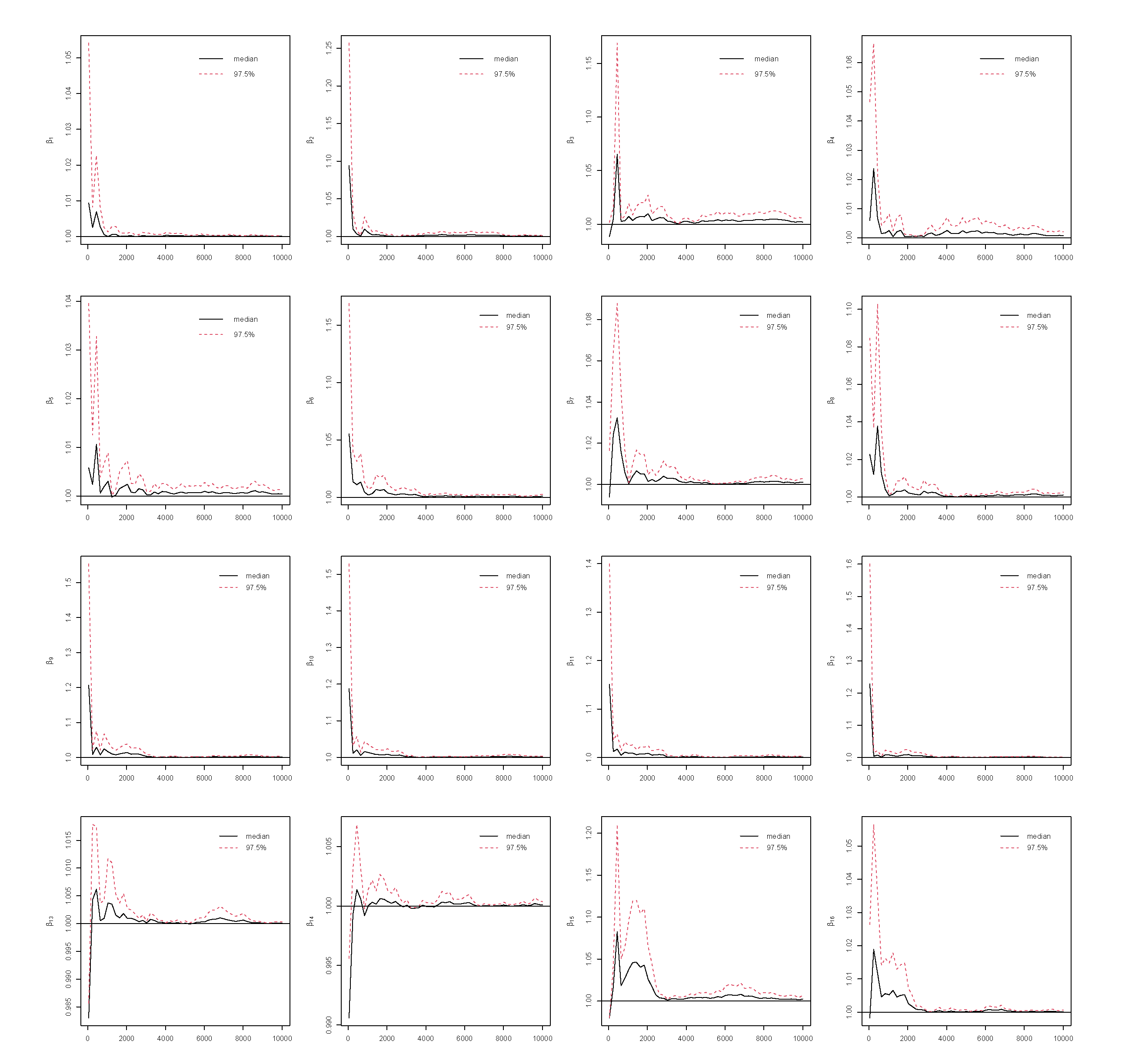
In this study, we use PSRF ≤ 1.1 ([26]) as the cut-off point which indicates that chains converge to a stationary distribution. In MCMC, the initial iterations are often affected by the choice of starting values and may not adequately represent draws from the stationary posterior distribution. To mitigate this influence and reduce bias in posterior estimation, these early samples are commonly discarded as burn-in iterations ([5]). In this study, the Gibbs sampling is implemented with 10,000 iterations with the first 5000 as burn-ins. The convergence of the MCMC chains after burn-ins has been checked for all predictors under the four coding strategies, which can be found in Figure A1, Figure A2, Figure A3 and Figure A4 in the Appendix. Take Race from dummy coding as an example in Figure 3. The PSRF trajectories for the three Race dummy variables corresponding to Non-Hispanic white, Non-Hispanic black, and other race categories, respectively. For each parameter, the median PSRF (solid black line) rapidly approaches and stabilizes near 1.00, and the upper 97.5% quantile (dashed red line) remains well below the commonly used threshold of 1.1 after early iterations. This pattern indicates good mixing and convergence of the Markov chains for all three race coefficients. The initial variability observed in the early iterations diminishes quickly, further supporting the conclusion that the chains have converged. These results suggest that posterior inference for the race-related coefficients is reliable and based on well-converged MCMC samples.
5. Discussion
In this study, we investigate the impact of coding strategies on categorical predictors in variable selection, prediction, and statistical inference with Bayesian LASSO in MEPS data. Comparisons against frequentist approaches such as linear regression and LASSO have also been performed. Our study complements existing work, such as [1], by adopting a Bayesian framework and incorporating formal statistical inference procedures into the analysis. Huang et al. ([1]) have also evaluated group LASSO as an alternative to LASSO on regression with categorical predictors, and concluded that group LASSO leads to overfitting few instead of all dummy predictors within the same group are needed. While we agree with their conclusion regarding the application of group LASSO, we want to point out that sparse group LASSO ([27,28]) is a promising regularization method that seeks to achieve sparsity on both group level and within group level. Therefore, sparse group LASSO type of methods are potentially promising in the scenario when selection of important categorical predictors within groups are of interest.
Due to heterogeneity of complex diseases such as multiple sclerosis and cancers, disease phenotypes of interest usually follow heavy-tailed distributions and have outlying observation. Therefore, robust statistical methods, especially robust regularization and variable selection methods that can safeguard against outliers and skewed distributions are demanded ([18]). Recently, the advantages of robust Bayesian variable selection methods over their frequentist counterparts, particularly in the context of statistical inference, have been investigated in [7]. It will be interesting to explore how robust Bayesian analysis can facilitate modeling with categorical predictors. For example, the robust Bayesian sparse group LASSO model proposed in [29] offers uncertainty quantification, which is typically unavailable in corresponding frequentist approaches ([27,28]). In future work, we also plan to extend the current methodology to other types of phenotypic traits, such as survival and longitudinal outcomes.
Author Contributions
Conceptualization, Xi Lu, Jieni Li, Rajender R. Aparasu and Cen Wu; methodology, Xi Lu and Cen Wu; software, Xi Lu and Nebil Yusuf; validation, Xi Lu, Jieni Li, Rajender R. Aparasu and Cen Wu; formal analysis, Xi Lu; investigation, Cen Wu; data curation, Jieni Li and Rajender R. Aparasu; writing—original draft preparation, Xi Lu; writing—review and editing, Xi Lu, Cen Wu, Jieni Li and Rajender R. Aparasu. All authors have read and agreed to the published version of the manuscript.
Funding
This research received no external funding.
Institutional Review Board Statement
The study was approved by the University of Houston’s Institutional Review Board under the exempt category.
Informed Consent Statement
Not applicable.
Data Availability Statement
The datasets generated during and/or analyzed during the current study are available from the corresponding author on reasonable request.
Conflicts of Interest
Rajender R. Aparasu has received research funding from Incyte, Novartis, Gilead, and Astellas outside the submitted work. The other authors declare no conflicts of interest.
Appendix A. Additional Results

Table A1.
Predicted scores for different coding strategies by linear regression.
| Education Level | Dummy | Deviation | Sequential | Helmert | Actual mean |
|---|---|---|---|---|---|
| No Degree | 46.0823 | 46.0823 | 46.0823 | 46.0823 | 46.0823 |
| High School Diploma/GED | 47.6153 | 47.6153 | 47.6153 | 47.6153 | 47.6153 |
| Bachelor’s Degree | 51.4337 | 51.4337 | 51.4337 | 51.4337 | 51.4337 |
| Master’s/Doctorate Degree | 51.4983 | 51.4983 | 51.4983 | 51.4983 | 51.4983 |
| Other Degree | 48.5679 | 48.5679 | 48.5679 | 48.5679 | 48.5679 |
Table A2.
Predicted scores for different coding strategies by LASSO.
| Education Level | Dummy | Deviation | Sequential | Helmert | Actual mean |
|---|---|---|---|---|---|
| No Degree | 59.6511 | 57.2106 | 59.6527 | 57.2065 | 46.0823 |
| High School Diploma/GED | 57.2106 | 58.3172 | 60.7578 | 58.3160 | 47.6153 |
| Bachelor’s Degree | 63.1154 | 58.3172 | 63.1909 | 60.7127 | 51.4337 |
| Master’s/Doctorate Degree | 63.8870 | 61.4876 | 63.9152 | 61.5013 | 51.4983 |
| Other Degree | 61.4729 | 59.0968 | 61.5856 | 59.1230 | 48.5679 |
Table A3.
Variable selection for different coding strategies by linear regression on MEPS data. Note: Variables with a white background were selected to be in the model, and variables with a gray background were not selected.
Table A3.
Variable selection for different coding strategies by linear regression on MEPS data. Note: Variables with a white background were selected to be in the model, and variables with a gray background were not selected.
| Variable | Dummy | Deviation | Sequential | Helmert |
|---|---|---|---|---|
| Marital Status | no–yes | no–Average | no–yes | yes–Average (no) |
| Sex | Female–Male | Female–Average | Female–Male | Male–Average (Female) |
| Race | Non-Hispanic White–Hispanic | Non-Hispanic White–Average | Non-Hispanic White–Hispanic | Hispanic–Average (White, Black, Other) |
| Non-Hispanic Black–Hispanic | Non-Hispanic Black–Average | Non-Hispanic Black–Hispanic | White–Average (Black, Other) | |
| Other–Hispanic | Other–Average | Other–Hispanic | Black–Other | |
| Region | Mid West–North East | Mid West–Average | Mid West–North East | North East–Average (Mid West, South, West) |
| South–North East | South–Average | South–North East | Mid West–Average (South, West) | |
| West–North East (Usual) | West–Average | West–North East | South–West | |
| Education | High School Diploma/GED–No Degree | High School Diploma/GED–Average | High School Diploma/GED–No Degree | No Degree–Average (HS/GED, Bachelor’s, Master’s/Doctorate, Other) |
| Bachelor’s Degree–No Degree | Bachelor’s Degree–Average | Bachelor’s Degree–No Degree | HS/GED–Average (Bachelor’s, Master’s/Doctorate, Other) | |
| Master’s/Doctorate–No Degree | Master’s/Doctorate–Average | Master’s/Doctorate–No Degree | Bachelor’s–Average (Master’s/Doctorate, Other) | |
| Other Degree–No Degree | Other Degree–Average | Other Degree–No Degree | Master’s/Doctorate–Other Degree | |
| Insurance | Public Only–Any Private | Public Only–Average | Public Only–Any Private | Any Private–Average (Public Only, Uninsured) |
| Coverage | Uninsured–Any Private | Uninsured–Average | Uninsured–Any Private | Public Only–Uninsured |
Table A4.
Variable selection for different coding strategies by LASSO on MEPS data. Note: Variables with a white background were selected to be in the model, and variables with a gray background were not selected.
Table A4.
Variable selection for different coding strategies by LASSO on MEPS data. Note: Variables with a white background were selected to be in the model, and variables with a gray background were not selected.
| Variable | Dummy | Deviation | Sequential | Helmert |
|---|---|---|---|---|
| Marital Status | no–yes | no–Average | no–yes | yes–Average (no) |
| Sex | Female–Male | Female–Average | Female–Male | Male–Average (Female) |
| Race | Non-Hispanic White–Hispanic | Non-Hispanic White–Average | Non-Hispanic White–Hispanic | Hispanic–Average (White, Black, Other) |
| Non-Hispanic Black–Hispanic | Non-Hispanic Black–Average | Non-Hispanic Black–Hispanic | White–Average (Black, Other) | |
| Other–Hispanic | Other–Average | Other–Hispanic | Black–Other | |
| Region | Mid West–North East | Mid West–Average | Mid West–North East | North East–Average (Mid West, South, West) |
| South–North East | South–Average | South–North East | Mid West–Average (South, West) | |
| West–North East (Usual) | West–Average | West–North East | South–West | |
| Education | High School Diploma/GED–No Degree | High School Diploma/GED–Average | High School Diploma/GED–No Degree | No Degree–Average (HS/GED, Bachelor’s, Master’s/Doctorate, Other) |
| Bachelor’s Degree–No Degree | Bachelor’s Degree–Average | Bachelor’s Degree–No Degree | HS/GED–Average (Bachelor’s, Master’s/Doctorate, Other) | |
| Master’s/Doctorate–No Degree | Master’s/Doctorate–Average | Master’s/Doctorate–No Degree | Bachelor’s–Average (Master’s/Doctorate, Other) | |
| Other Degree–No Degree | Other Degree–Average | Other Degree–No Degree | Master’s/Doctorate–Other Degree | |
| Insurance | Public Only–Any Private | Public Only–Average | Public Only–Any Private | Any Private–Average (Public Only, Uninsured) |
| Coverage | Uninsured–Any Private | Uninsured–Average | Uninsured–Any Private | Public Only–Uninsured |
Table A5.
Inference results with Bayesian LASSO on MEPS data. Note: Variable names followed with an underscore denote ordinal variables, which can be found in Table 6. Since the reference category differs across coding strategies, we use numbers for easier notation.
Table A5.
Inference results with Bayesian LASSO on MEPS data. Note: Variable names followed with an underscore denote ordinal variables, which can be found in Table 6. Since the reference category differs across coding strategies, we use numbers for easier notation.
| Dummy | Deviation | Sequential | Helmert | |||||||||||||
|---|---|---|---|---|---|---|---|---|---|---|---|---|---|---|---|---|
| Variable | Post. Median | Lower | Upper | Len. | Post. Median | Lower | Upper | Len. | Post. Median | Lower | Upper | Len. | Post. Median | Lower | Upper | Len. |
| intercept | 58.5066 | 58.3573 | 58.6596 | 0.3023 | 58.8036 | 58.6655 | 58.9429 | 0.2775 | 58.4924 | 58.3385 | 58.6492 | 0.3107 | 58.8056 | 58.6750 | 58.9272 | 0.2522 |
| ms | -11.0924 | -12.0778 | -10.1862 | 1.9166 | -11.0904 | -12.0813 | -10.1328 | 1.9789 | -11.0480 | -12.0527 | -10.0994 | 1.9533 | -11.0861 | -12.0527 | -10.0994 | 1.9533 |
| sex | -0.7173 | -0.8056 | -0.6260 | 0.1795 | -0.7119 | -0.8042 | -0.6221 | 0.1822 | -0.7186 | -0.8140 | -0.6235 | 0.1819 | -0.7185 | -0.8062 | -0.6255 | 0.1807 |
| race_1 | -0.4395 | -0.5665 | -0.3094 | 0.2570 | 0.6487 | 0.5316 | 0.7658 | 0.2342 | -0.4462 | -0.5764 | -0.3137 | 0.2627 | 0.8647 | 0.7072 | 1.0234 | 0.3162 |
| race_2 | -0.7137 | -0.8976 | -0.5380 | 0.3597 | 0.0075 | -0.0811 | 0.0969 | 0.1779 | -0.2734 | -0.4518 | -0.1031 | 0.3487 | 0.3339 | 0.1969 | 0.4722 | 0.2752 |
| race_3 | -0.6770 | -0.8987 | -0.4566 | 0.4422 | -0.3197 | -0.4531 | -0.1919 | 0.2613 | 0.0398 | -0.2090 | 0.2895 | 0.4985 | 0.0138 | -0.2306 | 0.2596 | 0.4902 |
| region_1 | -0.5054 | -0.6740 | -0.3321 | 0.3419 | 0.5404 | 0.4250 | 0.6573 | 0.2323 | -0.4951 | -0.6692 | -0.3334 | 0.3358 | 0.7201 | 0.5652 | 0.8781 | 0.3128 |
| region_2 | -0.7978 | -0.9489 | -0.6545 | 0.2944 | -0.2454 | -0.3499 | -0.1413 | 0.2086 | -0.2963 | -0.4398 | -0.1496 | 0.2902 | -0.0960 | -0.2354 | 0.0430 | 0.2784 |
| region_3 | -0.0048 | -0.1611 | 0.1526 | 0.3136 | -0.5262 | -0.6144 | -0.4399 | 0.1745 | 0.7932 | 0.6455 | 0.9357 | 0.2902 | -0.7552 | -0.9070 | -0.6029 | 0.3041 |
| education_1 | 1.4466 | 1.2754 | 1.6018 | 0.3265 | -2.1544 | -2.2973 | -2.0117 | 0.2857 | 1.4571 | 1.2942 | 1.6197 | 0.3255 | -2.6935 | -2.8741 | -2.5156 | 0.3586 |
| education_2 | 3.9013 | 3.6999 | 4.0903 | 0.3903 | 1.0065 | -1.0951 | -0.9199 | 0.1752 | 2.4536 | 2.3000 | 2.6107 | 0.3107 | -2.0591 | -2.1798 | -1.9395 | 0.2403 |
| education_3 | 4.6650 | 4.4398 | 4.8947 | 0.4549 | 1.3744 | 1.2580 | 1.4950 | 0.2369 | 0.7656 | 0.5509 | 0.9717 | 0.4208 | 0.4795 | 0.3045 | 0.6545 | 0.3501 |
| education_4 | 2.2389 | 2.0041 | 2.4732 | 0.4691 | 2.0987 | 1.9573 | 2.2408 | 0.2835 | -2.4233 | -2.6677 | -2.1722 | 0.4956 | 2.4073 | 2.1631 | 2.6559 | 0.4928 |
| inscov_1 | -3.5208 | -3.6525 | -3.3882 | 0.2643 | 1.4106 | 1.3237 | 1.5008 | 0.1771 | -3.5179 | -3.6501 | -3.3837 | 0.2664 | 2.1199 | 1.9825 | 2.2551 | 0.2726 |
| inscov_2 | -0.1096 | -0.3202 | 0.1044 | 0.4246 | -2.3115 | -2.4153 | -2.2062 | 0.2090 | 3.4049 | 3.1733 | 3.6339 | 0.4606 | -3.1994 | -3.4330 | -2.9731 | 0.4599 |
| age | -0.1365 | -0.1397 | -0.1335 | 0.0063 | -0.1353 | -0.1384 | -0.1323 | 0.0061 | -0.1363 | -0.1397 | -0.1330 | 0.0066 | -0.1354 | -0.1383 | -0.1323 | 0.0060 |
| eci | -1.8420 | -1.8754 | -1.8090 | 0.0664 | -1.8443 | -1.8773 | -1.8106 | 0.0667 | -1.8429 | -1.8758 | -1.8092 | 0.0666 | -1.8446 | -1.8771 | -1.8125 | 0.0646 |
Table A6.
Estimation results with linear regression on MEPS data. Note: Variable names followed with an underscore denote ordinal variables, which can be found in Table A3. Since the reference category differs across coding strategies, we use numbers for easier notation.
Table A6.
Estimation results with linear regression on MEPS data. Note: Variable names followed with an underscore denote ordinal variables, which can be found in Table A3. Since the reference category differs across coding strategies, we use numbers for easier notation.
| Dummy | Deviation | Sequential | Helmert | |||||||||||||
|---|---|---|---|---|---|---|---|---|---|---|---|---|---|---|---|---|
| Variable | Coef. | Lower | Upper | Len. | Coef. | Lower | Upper | Len. | Coef. | Lower | Upper | Len. | Coef. | Lower | Upper | Len. |
| intercept | 59.7027 | 59.4218 | 59.9835 | 0.5617 | 59.4063 | 59.2083 | 59.6044 | 0.3961 | 59.7027 | 59.2083 | 59.6044 | 0.3961 | 59.4063 | 59.2083 | 59.6044 | 0.3961 |
| ms | -11.145 | -12.1336 | -10.1565 | 1.9771 | -11.145 | -12.1336 | -10.1565 | 1.9771 | -11.145 | -12.1336 | -10.1565 | 1.9771 | -11.145 | -12.1336 | -10.1565 | 1.9771 |
| sex | -0.8176 | -0.9295 | -0.7057 | 0.2238 | -0.8176 | -0.9295 | -0.7057 | 0.2238 | -0.8176 | -0.9295 | -0.7057 | 0.2238 | -0.8176 | -0.9295 | -0.7057 | 0.2238 |
| race_1 | -0.6053 | -0.7655 | -0.4452 | 0.3202 | 0.5958 | 0.4764 | 0.7152 | 0.2388 | -0.6053 | 0.4764 | 0.7152 | 0.2388 | 0.7944 | 0.6352 | 0.9536 | 0.3184 |
| race_2 | -0.8954 | -1.0964 | -0.6944 | 0.4020 | -0.0095 | -0.1031 | 0.0841 | 0.1872 | -0.2901 | -0.1031 | 0.0841 | 0.1872 | 0.2836 | 0.1376 | 0.4296 | 0.2920 |
| race_3 | -0.8825 | -1.1188 | -0.6462 | 0.4726 | -0.2996 | -0.4307 | -0.1685 | 0.2622 | 0.0129 | -0.4307 | -0.1685 | 0.2622 | -0.0129 | -0.2645 | 0.2386 | 0.5031 |
| region_1 | -0.8166 | -1.0032 | -0.6299 | 0.3732 | 0.5751 | 0.4582 | 0.6921 | 0.2339 | -0.8166 | 0.4582 | 0.6921 | 0.2339 | 0.7668 | 0.6109 | 0.9228 | 0.3118 |
| region_2 | -1.1297 | -1.3013 | -0.9580 | 0.3433 | -0.2414 | -0.3460 | -0.1368 | 0.2092 | -0.3131 | -0.3460 | -0.1368 | 0.2092 | -0.0746 | -0.2173 | 0.0681 | 0.2855 |
| region_3 | -0.3543 | -0.5365 | -0.1721 | 0.3644 | -0.5545 | -0.6446 | -0.4644 | 0.1802 | 0.7754 | -0.6446 | -0.4644 | 0.1802 | -0.7754 | -0.9235 | -0.6273 | 0.2962 |
| education_1 | 1.1349 | 0.9592 | 1.3107 | 0.3514 | -2.2002 | -2.3424 | -2.0581 | 0.2843 | 1.1349 | -2.3424 | -2.0581 | 0.2843 | -2.7503 | -2.9280 | -2.5726 | 0.3554 |
| education_2 | 3.5723 | 3.3631 | 3.7815 | 0.4183 | -1.0653 | -1.1568 | -0.9739 | 0.1829 | 2.4374 | -1.1568 | -0.9739 | 0.1829 | -2.1538 | -2.2807 | -2.0270 | 0.2537 |
| education_3 | 4.3592 | 4.1245 | 4.5940 | 0.4696 | 1.3720 | 1.2529 | 1.4912 | 0.2383 | 0.7870 | 1.2529 | 1.4912 | 0.2383 | 0.4253 | 0.2506 | 0.6000 | 0.3494 |
| education_4 | 1.9348 | 1.6928 | 2.1767 | 0.4839 | 2.1590 | 2.0153 | 2.3027 | 0.2873 | -2.4245 | 2.0153 | 2.3027 | 0.2873 | 2.4245 | 2.1813 | 2.6677 | 0.4864 |
| inscov_1 | -3.6080 | -3.7423 | -3.4737 | 0.2686 | 1.3256 | 1.2321 | 1.4192 | 0.1871 | -3.6080 | 1.2321 | 1.4192 | 0.1871 | 1.9885 | 1.8482 | 2.1288 | 0.2806 |
| inscov_2 | -0.3689 | -0.5891 | -0.1488 | 0.4403 | -2.2824 | -2.3857 | -2.1790 | 0.2068 | 3.2391 | -2.3857 | -2.1790 | 0.2068 | -3.2391 | -3.4721 | -3.0060 | 0.4661 |
| age | -0.1439 | -0.1474 | -0.1403 | 0.0071 | -0.1439 | -0.1474 | -0.1403 | 0.0071 | -0.1439 | -0.1474 | -0.1403 | 0.0071 | -0.1439 | -0.1474 | -0.1403 | 0.0071 |
| eci | -1.8275 | -1.8606 | -1.7945 | 0.0661 | -1.8275 | -1.8606 | -1.7945 | 0.0661 | -1.8275 | -1.8606 | -1.7945 | 0.0661 | -1.8275 | -1.8606 | -1.7945 | 0.0661 |
Table A7.
Estimation results with LASSO on MEPS data. Note: Variable names followed with an underscore denote ordinal variables, which can be found in Table A4. Since the reference category differs across coding strategies, we denote them with numbers for easier notation.
Table A7.
Estimation results with LASSO on MEPS data. Note: Variable names followed with an underscore denote ordinal variables, which can be found in Table A4. Since the reference category differs across coding strategies, we denote them with numbers for easier notation.
| Variable | Dummy | Deviation | Sequential | Helmert |
|---|---|---|---|---|
| intercept | 59.6511 | 59.3654 | 59.6527 | 59.3719 |
| ms | -11.0354 | -10.9795 | -10.9707 | -10.9469 |
| sex | -0.8042 | -0.7995 | -0.8012 | -0.7973 |
| race_1 | -0.5241 | 0.5588 | -0.5747 | 0.7473 |
| race_2 | -0.8217 | 0.0000 | -0.2777 | 0.2457 |
| race_3 | -0.7934 | -0.2817 | 0.0000 | -0.0053 |
| region_1 | -0.7520 | 0.5277 | -0.8007 | 0.7357 |
| region_2 | -1.0672 | -0.2176 | -0.2784 | -0.0397 |
| region_3 | -0.2807 | -0.5362 | 0.7359 | -0.7555 |
| education_1 | 1.0369 | -2.1548 | 1.1051 | -2.7067 |
| education_2 | 3.4643 | -1.0482 | 2.4331 | -2.1297 |
| education_3 | 4.2459 | 1.3494 | 0.7243 | 0.4006 |
| education_4 | 1.8218 | 2.1222 | -2.3296 | 2.3783 |
| inscov_1 | -3.6080 | 1.3197 | -3.5880 | 1.9838 |
| inscov_2 | -0.3409 | -2.2775 | 3.1820 | -3.2296 |
| age | -0.1437 | -0.1435 | -0.1435 | -0.1433 |
| eci | -1.8271 | -1.8272 | -1.8276 | -1.8267 |
Appendix B. Assessment of the Convergence of MCMC Chains
Figure A1.
Potential scale reduction factor (PSRF) against iterations for all coefficients under the dummy coding strategy. Note: The black line denotes the PSRF and the red dotted line indicates the upper limit of the 95% confidence interval for the PSRF.
Figure A1.
Potential scale reduction factor (PSRF) against iterations for all coefficients under the dummy coding strategy. Note: The black line denotes the PSRF and the red dotted line indicates the upper limit of the 95% confidence interval for the PSRF.

Figure A2.
Potential scale reduction factor (PSRF) against iterations for all coefficients under the deviation coding strategy. Note: The black line denotes the PSRF and the red dotted line indicates the upper limit of the 95% confidence interval for the PSRF.
Figure A2.
Potential scale reduction factor (PSRF) against iterations for all coefficients under the deviation coding strategy. Note: The black line denotes the PSRF and the red dotted line indicates the upper limit of the 95% confidence interval for the PSRF.

Figure A3.
Potential scale reduction factor (PSRF) against iterations for all coefficients under the sequential coding strategy. Note: The black line denotes the PSRF and the red dotted line indicates the upper limit of the 95% confidence interval for the PSRF.
Figure A3.
Potential scale reduction factor (PSRF) against iterations for all coefficients under the sequential coding strategy. Note: The black line denotes the PSRF and the red dotted line indicates the upper limit of the 95% confidence interval for the PSRF.

Figure A4.
Potential scale reduction factor (PSRF) against iterations for all coefficients under the Helmert coding strategy. Note: The black line denotes the PSRF and the red dotted line indicates the upper limit of the 95% confidence interval for the PSRF.
Figure A4.
Potential scale reduction factor (PSRF) against iterations for all coefficients under the Helmert coding strategy. Note: The black line denotes the PSRF and the red dotted line indicates the upper limit of the 95% confidence interval for the PSRF.
References
- Huang, Y.; Tibbe, T.D.; Tang, A.; Montoya, A.K. Lasso and Group Lasso with Categorical Predictors: Impact of Coding Strategy on Variable Selection and Prediction. Journal of Behavioral Data Science 2023, 3, 15–42. [Google Scholar] [CrossRef]
- James, G.; Witten, D.; Hastie, T.; Tibshirani. , R. An Introduction to Statistical Learning. Springer 2021. [Google Scholar]
- Tibshirani, R. Regression shrinkage and selection via the lasso. Journal of the Royal Statistical Society. Series B (Methodological) 1996, 58, 267–288. [Google Scholar] [CrossRef]
- Lu, X.; Fan, K.; Ren, J.; Wu, C. Identifying gene–environment interactions with robust marginal Bayesian variable selection. Frontiers in Genetics 2021, 12, 667074. [Google Scholar] [CrossRef]
- Gelman, A.; Carlin, J.B.; Stern, H.S.; Rubin, D.B. Bayesian data analysis; Chapman and Hall/CRC, 1995.
- Park, T.; Casella, G. The Bayesian Lasso. Journal of the American Statistical Association 2008, 103, 681–686. [Google Scholar] [CrossRef]
- Fan, K.; Subedi, S.; Yang, G.; Lu, X.; Ren, J.; Wu, C. Is Seeing Believing? A Practitioner’s Perspective on High-Dimensional Statistical Inference in Cancer Genomics Studies. Entropy 2024, 26, 794. [Google Scholar] [CrossRef]
- Scalfari, A.; Neuhaus, A.; Daumer, M.; DeLuca, G.C.; Muraro, P.A.; Ebers, G.C. Early Relapses, Onset of Progression, and Late Outcome in Multiple Sclerosis. JAMA Neurol 2013, 70, 214–222. [Google Scholar] [CrossRef]
- Bergamaschi, R.; Quaglini, S.; Trojano, M.; Amato, M.P.; Tavazzi, E.; Paolicelli, D.; Zipoli, V.; Romani, A.; Fuiani, A.; Portaccio, E.; et al. Early prediction of the long term evolution of multiple sclerosis: the Bayesian Risk Estimate for Multiple Sclerosis (BREMS) score. J Neurol Neurosurg Psychiatry 2007, 78, 757–759. [Google Scholar] [CrossRef]
- Bebo, B.; Cintina, I.; LaRocca, N.; Ritter, L.; Talente, B.; Hartung, D.; Ngorsuraches, S.; Wallin, M.; Yang, G. The Economic Burden of Multiple Sclerosis in the United States: Estimate of Direct and Indirect Costs. Neurology 2022, 98, e1810–e1817. [Google Scholar] [CrossRef]
- Rezaee, M.; Keshavarz, K.; Izadi, S.; Jafari, A.; Ravangard, R. Economic burden of multiple sclerosis: a cross-sectional study in Iran. Health Economics Review volume 2022, 12. [Google Scholar] [CrossRef]
- Li, J.; Zakeri, M.; Hutton, G.J.; Aparasu, R.R. Health-related quality of life of patients with multiple sclerosis: analysis of ten years of national data. Multiple Sclerosis and Related Disorders 2022, 66, 104019. [Google Scholar] [CrossRef]
- Moore, B.J.; White, S.; Washington, R.; Coenen, N.; Elixhauser, A. Identifying increased risk of readmission and in-hospital mortality using hospital administrative data: the AHRQ Elixhauser Comorbidity Index. Medical care 2017, 55, 698–705. [Google Scholar] [CrossRef] [PubMed]
- Kugler, K.C.; Dziak, J.J.; Trail, J. Coding and interpretation of effects in analysis of data from a factorial experiment. In Optimization of behavioral, biobehavioral, and biomedical interventions: Advanced topics; Springer, 2018; pp. 175–205.
- UCLA Statistical Consulting Group. Coding systems for categorical variables in regression analysis. https://stats.oarc.ucla.edu/r/library/r-library-contrast-coding-systems-for-categorical-variables/. Accessed: 2025-08-12.
- Hayes, A.F.; Preacher, K.J. Statistical mediation analysis with a multicategorical independent variable. British journal of mathematical and statistical psychology 2014, 67, 451–470. [Google Scholar] [CrossRef] [PubMed]
- McNeish, D. On using Bayesian methods to address small sample problems. Structural Equation Modeling: A Multidisciplinary Journal 2016, 23, 750–773. [Google Scholar] [CrossRef]
- Wu, C.; Ma, S. A selective review of robust variable selection with applications in bioinformatics. Briefings in bioinformatics 2015, 16, 873–883. [Google Scholar] [CrossRef]
- Lockhart, R.; Taylor, J.; Tibshirani, R.J.; Tibshirani, R. A significance test for the lasso. Annals of statistics 2014, 42, 413. [Google Scholar] [CrossRef]
- Lee, J.D.; Sun, D.L.; Sun, Y.; Taylor, J.E. Exact post-selection inference, with application to the lasso 2016.
- Zhang, C.H.; Zhang, S.S. Confidence intervals for low dimensional parameters in high dimensional linear models. Journal of the Royal Statistical Society Series B: Statistical Methodology 2014, 76, 217–242. [Google Scholar] [CrossRef]
- Javanmard, A.; Montanari, A. Confidence intervals and hypothesis testing for high-dimensional regression. The Journal of Machine Learning Research 2014, 15, 2869–2909. [Google Scholar]
- Dezeure, R.; Bühlmann, P.; Meier, L.; Meinshausen, N. High-dimensional inference: confidence intervals, p-values and R-software hdi. Statistical science 2015, pp. 533–558.
- Cowles, M.K.; Carlin, B.P. Markov chain Monte Carlo convergence diagnostics: a comparative review. Journal of the American statistical Association 1996, 91, 883–904. [Google Scholar] [CrossRef]
- Brooks, S.P.; Gelman, A. General methods for monitoring convergence of iterative simulations. Journal of computational and graphical statistics 1998, 7, 434–455. [Google Scholar] [CrossRef]
- Gelman, A.and Carlin, J.; Stern, H.; Dunson, D.; Vehtari, A.; Rubin, D. Bayesian Data Analysis. Chapman and Hall/CRC 2004.
- Simon, N.; Friedman, J.; Hastie, T.; Tibshirani, R. A sparse-group lasso. Journal of computational and graphical statistics 2013, 22, 231–245. [Google Scholar] [CrossRef]
- Friedman, J.; Hastie, T.; Tibshirani, R. A note on the group lasso and a sparse group lasso. arXiv preprint arXiv:1001.0736, arXiv:1001.0736 2010.
- Ren, J.; Zhou, F.; Li, X.; Ma, S.; Jiang, Y.; Wu, C. Robust Bayesian variable selection for gene–environment interactions. Biometrics 2023, 79, 684–694. [Google Scholar] [CrossRef]
Figure 1.
Posterior distributions of to for the simulated data. The grey dashed lines denote the lower and upper bounds of the 95% credible interval, and the blue solid line represents the median.
Figure 1.
Posterior distributions of to for the simulated data. The grey dashed lines denote the lower and upper bounds of the 95% credible interval, and the blue solid line represents the median.
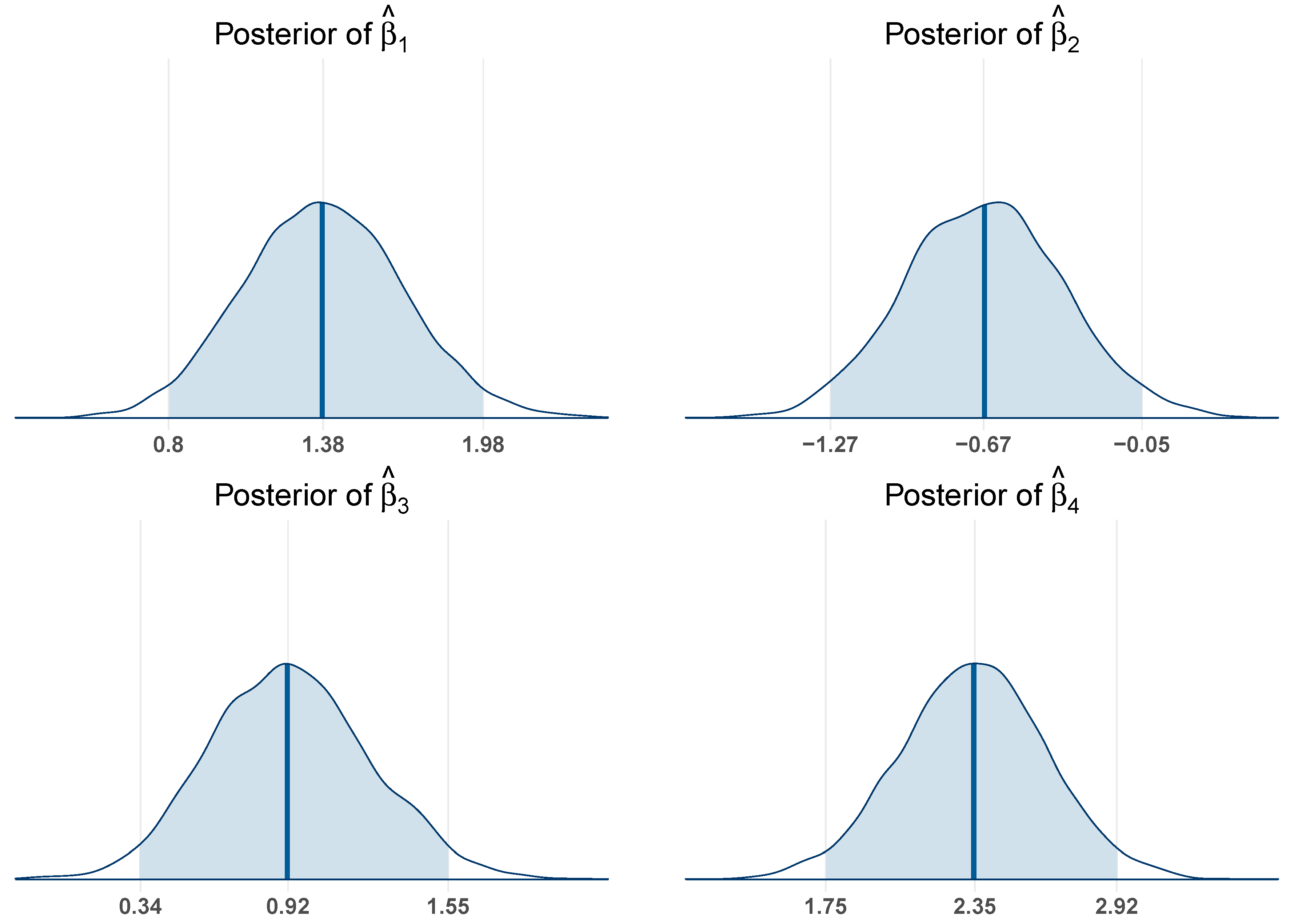
Figure 2.
Posterior distributions of the regression coefficients associated with Race under dummy coding. The grey dashed lines denote the lower and upper bounds of the 95% credible interval, and the blue solid line represents the median.
Figure 2.
Posterior distributions of the regression coefficients associated with Race under dummy coding. The grey dashed lines denote the lower and upper bounds of the 95% credible interval, and the blue solid line represents the median.
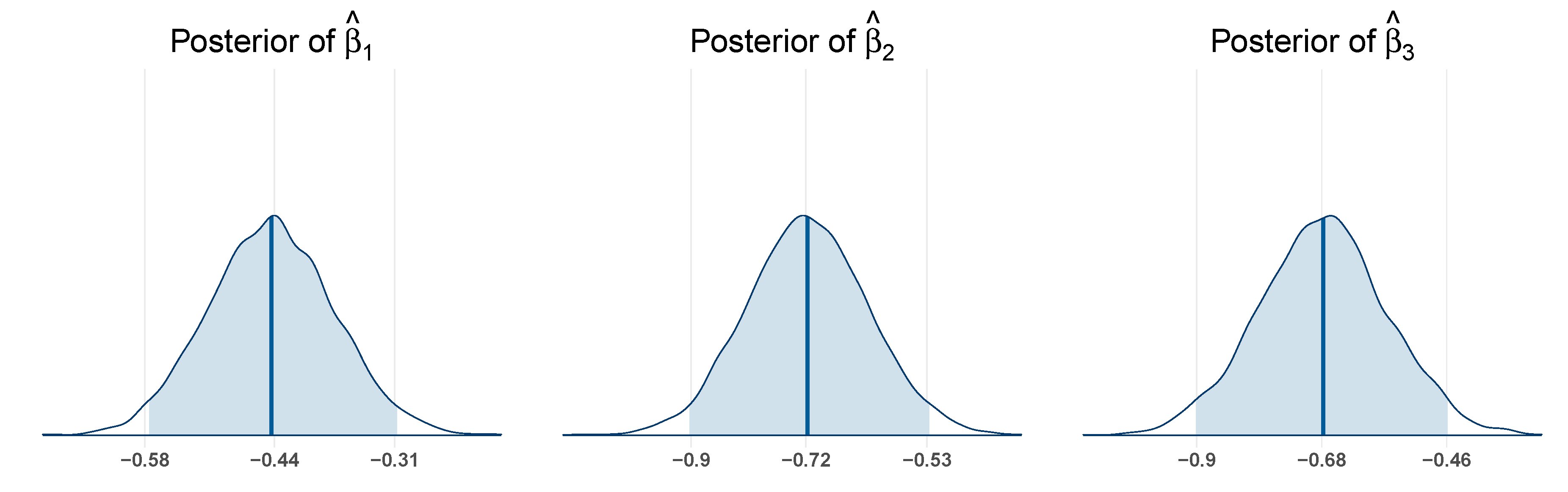
Figure 3.
Potential scale reduction factor (PSRF) against iterations for the three coefficients associated with Race under dummy coding. The black line shows the PSRF, and the red dotted line marks the upper limit of the 95% confidence interval.
Figure 3.
Potential scale reduction factor (PSRF) against iterations for the three coefficients associated with Race under dummy coding. The black line shows the PSRF, and the red dotted line marks the upper limit of the 95% confidence interval.
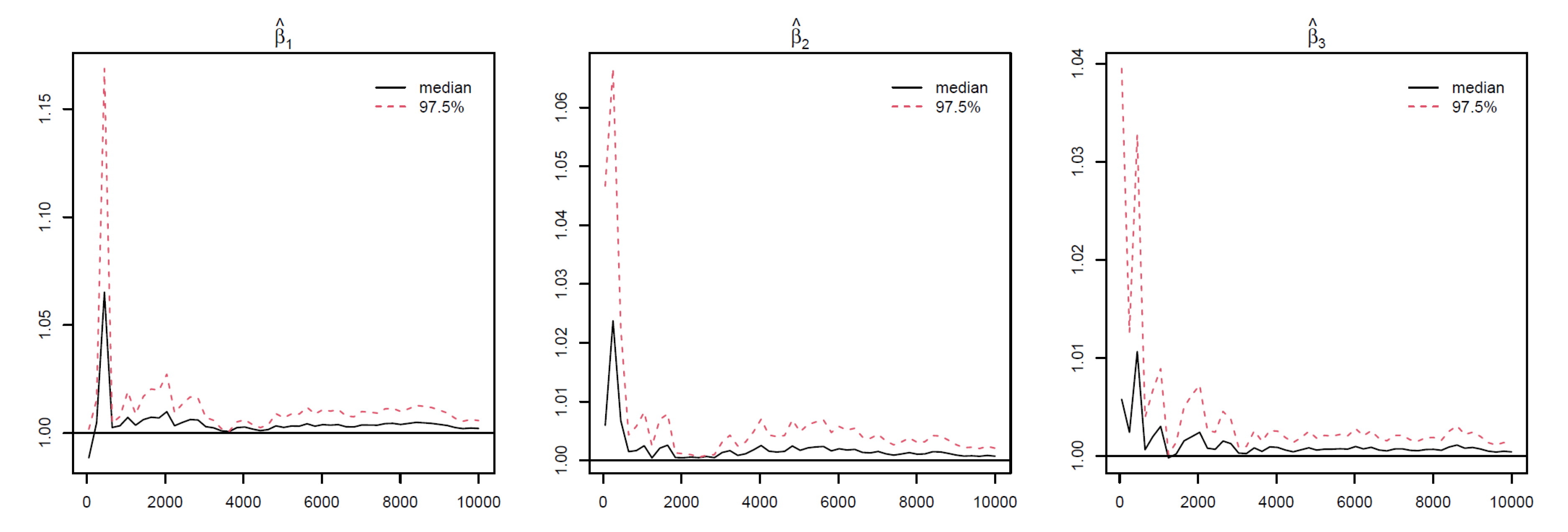
Table 1.
Dummy coding for education levels. Note: One category is set as a reference, and other categories are compared to it. No degree is selected as the reference group (coded 0 on all indicators).
Table 1.
Dummy coding for education levels. Note: One category is set as a reference, and other categories are compared to it. No degree is selected as the reference group (coded 0 on all indicators).
| Education Level | ||||
|---|---|---|---|---|
| No Degree | 0 | 0 | 0 | 0 |
| High School Diploma or GED | 1 | 0 | 0 | 0 |
| Bachelor’s Degree | 0 | 1 | 0 | 0 |
| Master’s or Doctorate Degree | 0 | 0 | 1 | 0 |
| Other Degree | 0 | 0 | 0 | 1 |
Table 2.
Deviation coding for education levels. Note: Compares each category with the mean rather than a single reference category. Other degree is selected as the omitted category (coded on all indicators).
Table 2.
Deviation coding for education levels. Note: Compares each category with the mean rather than a single reference category. Other degree is selected as the omitted category (coded on all indicators).
| Education Level | ||||
|---|---|---|---|---|
| No Degree | 1 | 0 | 0 | 0 |
| High School Diploma or GED | 0 | 1 | 0 | 0 |
| Bachelor’s Degree | 0 | 0 | 1 | 0 |
| Master’s or Doctorate Degree | 0 | 0 | 0 | 1 |
| Other Degree | -1 | -1 | -1 | -1 |
Table 3.
Sequential coding for education levels. Note: Compares each category to the one before it in an ordered fashion. Each subsequent category scores 1 on one more indicator than the previous.
Table 3.
Sequential coding for education levels. Note: Compares each category to the one before it in an ordered fashion. Each subsequent category scores 1 on one more indicator than the previous.
| Education Level | ||||
|---|---|---|---|---|
| No Degree | 0 | 0 | 0 | 0 |
| High School Diploma or GED | 1 | 0 | 0 | 0 |
| Bachelor’s Degree | 1 | 1 | 0 | 0 |
| Master’s or Doctorate Degree | 1 | 1 | 1 | 0 |
| Other Degree | 1 | 1 | 1 | 1 |
Table 4.
Helmert coding for education levels. Note: Each category is compared to the average of all higher categories.
Table 4.
Helmert coding for education levels. Note: Each category is compared to the average of all higher categories.
| Education Level | ||||
|---|---|---|---|---|
| No Degree | 0 | 0 | 0 | |
| High School Diploma or GED | 0 | 0 | ||
| Bachelor’s Degree | 0 | |||
| Master’s or Doctorate Degree | ||||
| Other Degree |
Table 5.
Bayesian linear regression estimates for different coding strategies.
| Coefficient | Dummy | Deviation | Sequential | Helmert |
|---|---|---|---|---|
| 2.0982 | 2.5409 | 2.1038 | 2.5411 | |
| 1.3411 | -0.4512 | 1.3418 | -0.5625 | |
| -1.0812 | 0.9021 | -2.4029 | 1.0504 | |
| 0.2286 | -1.5095 | 1.2956 | -2.0459 | |
| 1.7198 | -0.2159 | 1.4903 | -1.4811 |
Table 6.
Variable selection for different coding strategies by Bayesian LASSO on MEPS data. Note: Variables with a white background were selected to be in the model, and variables with a gray background were not selected.
Table 6.
Variable selection for different coding strategies by Bayesian LASSO on MEPS data. Note: Variables with a white background were selected to be in the model, and variables with a gray background were not selected.
| Variable | Dummy | Deviation | Sequential | Helmert |
|---|---|---|---|---|
| MS Status | no–yes | no–Average | no–yes | yes–Average (no) |
| Sex | Female–Male | Female–Average | Female–Male | Male–Average (Female) |
| Race | Non-Hispanic White–Hispanic | Non-Hispanic White–Average | Non-Hispanic White–Hispanic | Hispanic–Average (Non-Hispanic White, Non-Hispanic Black, Other) |
| Non-Hispanic Black–Hispanic | Non-Hispanic Black–Average | Non-Hispanic Black–Hispanic | Non-Hispanic White–Average (Non-Hispanic Black, Other) | |
| Other–Hispanic | Other–Average | Other–Hispanic | Non-Hispanic Black–Other | |
| Region | Mid West–North East | Mid West–Average | Mid West–North East | North East–Average (Mid West, South, West) |
| South–North East | South–Average | South–North East | Mid West–Average (South, West) | |
| West–North East (Usual) | West–Average | West–North East | South–West | |
| Education | High School Diploma/GED–No Degree | High School Diploma/GED–Average | High School Diploma/GED–No Degree | No Degree–Average (High School Diploma/GED, Bachelor’s, Master’s/Doctorate, Other) |
| Bachelor’s Degree–No Degree | Bachelor’s Degree–Average | Bachelor’s Degree–No Degree | High School Diploma/GED–Average (Bachelor’s, Master’s/Doctorate, Other) | |
| Master’s/Doctorate–No Degree | Master’s/Doctorate–Average | Master’s/Doctorate–No Degree | Bachelor’s Degree–Average (Master’s/Doctorate, Other) | |
| Other Degree–No Degree | Other Degree–Average | Other Degree–No Degree | Master’s/Doctorate–Other Degree | |
| Insurance | Public Only–Any Private | Public Only–Average | Public Only–Any Private | Any Private–Average (Public Only, Uninsured) |
| Coverage | Uninsured–Any Private | Uninsured–Average | Uninsured–Any Private | Public Only–Uninsured |
Table 7.
Predicted scores for different coding strategies by Bayesian LASSO. Note: The last column is the actual mean of each category.
Table 7.
Predicted scores for different coding strategies by Bayesian LASSO. Note: The last column is the actual mean of each category.
| Education Level | Dummy | Deviation | Sequential | Helmert | Actual mean |
|---|---|---|---|---|---|
| No Degree | 45.7169 | 46.0027 | 45.7132 | 46.0042 | 46.0823 |
| High School Diploma/GED | 47.6149 | 47.5916 | 47.6170 | 47.5893 | 47.6153 |
| Bachelor’s Degree | 51.4306 | 51.3722 | 51.4324 | 51.3734 | 51.4337 |
| Master’s/Doctorate Degree | 51.4991 | 51.4014 | 51.4980 | 51.4010 | 51.4983 |
| Other Degree | 48.5689 | 48.4416 | 48.5656 | 48.4481 | 48.5679 |
Table 8.
Prediction error with Bayesian LASSO, LASSO, and linear regression using different coding strategies.
Table 8.
Prediction error with Bayesian LASSO, LASSO, and linear regression using different coding strategies.
| Dummy | Deviation | Sequential | Helmert | |
|---|---|---|---|---|
| Bayesian LASSO | 6.6268 | 6.6247 | 6.6247 | 6.6247 |
| LASSO | 6.6130 | 6.6131 | 6.6134 | 6.6134 |
| Linear Regression | 6.6132 | 6.6132 | 6.6132 | 6.6132 |
Disclaimer/Publisher’s Note: The statements, opinions and data contained in all publications are solely those of the individual author(s) and contributor(s) and not of MDPI and/or the editor(s). MDPI and/or the editor(s) disclaim responsibility for any injury to people or property resulting from any ideas, methods, instructions or products referred to in the content. |
© 2025 by the authors. Licensee MDPI, Basel, Switzerland. This article is an open access article distributed under the terms and conditions of the Creative Commons Attribution (CC BY) license (http://creativecommons.org/licenses/by/4.0/).
Copyright: This open access article is published under a Creative Commons CC BY 4.0 license, which permit the free download, distribution, and reuse, provided that the author and preprint are cited in any reuse.


