
Submitted:
19 August 2025
Posted:
21 August 2025
You are already at the latest version
Abstract
This work develops a coupled simulation framework between a 1-D thermofluid network process model and a 3-D CFD air-side model of a natural draft direct dry cooling system (NDDDCS) for a supercritical carbon dioxide (sCO2) power cycle. The method leverages the computational efficiency of the network model to capture sCO₂-side property distributions within the heat exchanger tubes, while harnessing the high-fidelity capabilities of CFD to resolve intricate airflow phenomena on the air-side. An NDDDCS sized for a 50 MWe sCO2 application is simulated under no-wind conditions. Heat exchangers, serving both the precooler (PC) and intercooler (IC) heat loads, are included in the same cooling tower, featuring vertically arranged tube banks around the circumference. Results show that the model captures airflow effects such as recirculation at the heat exchangers and flow separation from the internal tower walls, which reduce the overall air mass flow rate by 6.25 % and heat transfer rate by 13.85 %, in comparison to a previous 1-D model, raising the sCO2-side outlet temperatures. Furthermore, the model investigates the variation in system performance of a lumped configuration, where the PC and IC tube banks are grouped, and an alternating configuration, where the tube banks are interspersed. The alternating configuration yields a relative performance increase of 1.88 % in the air mass flow rate and 1.02 % in heat transfer, as chaotic mixing and swirling flows are minimised, producing more uniform airflow through the tower. To assess whether implementing this alternating arrangement is justified, performance under crosswind conditions should be investigated.
Keywords:
natural draft direct dry cooling system
; supercritical CO2
; computational fluid dynamics
; process modelling
; co-simulation
1. Introduction
As global energy systems transition toward sustainable technologies, finding a means to address variability and dispatchability issues related to renewable options is necessary. Here concentrated solar power (CSP) applications have a definitive advantage as these systems can integrate with thermal energy storage which can be used during adverse operating conditions to ensure stable energy generation [1,2]. CSP plants need larger initial capital investment in comparison to other renewable alternatives such as photovoltaic solar or wind turbines [3]. To potentially alleviate this disadvantage, researchers have proposed integrating supercritical carbon dioxide (sCO2) Brayton cycles into power blocks for these applications, as this technology offers both superior operating efficiencies and reduced equipment costs [4]. The adoptability of sCO2 cycles into CSP is further emphasized by the reduced component sizes required when utilising dry cooling technologies [5]. This can prove to be beneficial for plant operation by minimising water consumption given that CSP plants are normally located in semi-arid to dry regions where water is scarce.
Mechanical draft air-cooled condensers (ACCs) or indirect natural draft dry cooling systems are typically used in thermal power generation using steam as working fluid. Both systems present a list of advantages and disadvantages faced during construction and operational phases. For example, ACCs consume a significant amount of parasitic power in the fan drive trains which also need regular maintenance and inspections, adding to operation cost [6]. Still, the direct condensation from ACCs yields high operating thermal efficiencies. On the other hand, the ease of operation of the indirect natural draft counter parts reduces auxiliary power, but high material and construction costs along with added system complexity, from the shell-and-tube condensers and pumping networks, reduce their favourability. Natural draft direct dry cooling systems (NDDDCSs) aim to combine the benefits of both dry cooling technologies by using the reduced operational complexity of indirect systems along with the higher associated efficiencies from the direct cooling of ACCs. This technology can therefore be explored for sCO2 cycle applications by determining overall system performance and resulting effects on cycle operation. However, during cooling of sCO2 large variations in thermophysical properties cause heat transfer and pressure drops to be highly irregular, necessitating modelling techniques to include discretised heat exchanger networks to estimate correct thermofluid behaviour. Multiple studies have integrated discretised heat exchanger networks into different dry cooling technologies. However, since this work focusses specifically on natural draft cooling systems, only studies investigating this configuration will be highlighted, and relevant recommendations from the conclusions will be incorporated into the present analysis.
One-dimensional (1-D) numerical models developed by Duniam, et al. [7] and Ehsan, et al. [8] compare direct and indirect natural draft dry cooling systems for sCO2 applications. The results from both studies confirm that the direct sCO2 to air heat transfer option requires a significantly smaller cooling tower and total heat exchanger area to reject the cycle heat load. Furthermore, Duniam, et al. [7] employed a direct cooling model to investigate how ambient temperature variations affect recompression cycle performance. For ambient temperatures below the design point, they incorporated a bypass arrangement to prevent the sCO2 from overcooling and maintain stable cycle operation. For ambient temperatures beyond the design point value, cycle efficiency is significantly affected by the additional work required by the compressors to operate at elevated inlet conditions. This emphasises the sensitivity of the sCO2 cycle to changes in ambient conditions and therefore consideration should be given to the climate where proposed future plants are to be constructed.
Lock, et al. [9] investigate the performance of an NDDDCS for a recompression sCO2 cycle with a 1-D element-based discretised heat exchanger model. In this investigation, the authors of the study compare different internal forced convection heat transfer correlations and reveal that typical constant property correlations significantly underpredict the convective heat transfer behaviour within the heat exchanger tubes, resulting in overdesigned heat exchangers. The study recommends the use of correlations developed by Wang, et al. [10,11], as these coefficients were derived from heat transfer behaviour of sCO2 in large diameter tubes.
In previous work by the authors of this paper, the design and off-design operation of an NDDDCS is investigated [12]. Preliminary work uses a lumped parameter modelling approach, with linearly averaged properties across the heat exchanger, to select a cooling system geometry. A parametric study was completed by varying cooling tower geometric ratios as well as total heat exchanger passes, with the result aimed at minimizing the total lost work through the heat exchangers as well as total system material cost. The most cost-effective system geometry is incorporated into a discretised 1-D heat exchanger model solving with the thermofluid network modelling (TNM) approach, which addresses the limitations of lumped parameter modelling approaches. In this context of sCO2 heat transfer modelling, the lumped approach consistently overpredicts heat transfer performance in both the precooler (PC) and intercooler (IC) since the correct property gradients are not accounted for, highlighting its inadequacy for capturing the underlying behaviour [12].
However, the aforementioned studies rely on 1-D methods, which, due to their limited fidelity, are incapable of capturing detailed flow airflow behaviours. Strydom [13] reveals that 1-D modelling used to predict steady state NDDDCS performance for Rankine cycles consistently overpredict performance metrics under no-wind conditions in comparison to 3-D computational fluid dynamics (CFD) models. This results from the inability of 1-D methods to account for phenomena such as recirculation vortices in front of the vertically arranged heat exchanger tube banks and flow separation from the internal cooling tower shell, as detailed in [14]. To the best of the authors’ knowledge, currently no study employs an air-side CFD model to investigate the performance of an NDDDCS for an sCO2 application. Therefore, studies from literature which have applied such methods to steam applications are insightful, and their modelling techniques and recommendations are evaluated in the following discussion.
Kong, et al. [15,16,17] produced multiple papers on this topic with primary focus on large coal-fired power plants. The numerical models developed in their work consisted of utilising radiator model of ANSYS Fluent to represent the finned tube heat exchangers in the system geometry. Here the required energy- and momentum source terms are added to the respective transport equations to model the air flow through the heat exchangers. In the first publication from Kong, et al. [15], a tower with horizontally arranged heat exchanger tube bundles within the tower base is compared to a configuration with vertical bundles around the tower circumference. Here the vertical arrangements outperform the horizontal geometry under no-wind and windy conditions. Following up on this work, the authors determined that for a heat exchanger with the same frontal area, an annularly arranged geometry obtains better performance compared to one with an apex angle of 60° between each tube bank [16]. These changes in geometry can be applied to investigations involving sCO2 to reduce the cooling tower size while enhancing performance.
Strydom, et al. [14] extend the investigation of NDDDCS applications to medium scale CSP plants and smaller scale desalination plants. The CFD model developed in their work uses a porous media to represent the vertical heat exchangers arranged around the circumference of the cooling tower with detailed energy- and momentum source terms included. Notably the momentum source term used in [14] also includes the air flow resistance encountered by inlet louvres and tower supports as recommended by Kröger [18], which is neglected in the work from [15,16,17]. Furthermore, the model from [14] includes detailed flat finned tube heat exchanger characteristics along with the steam side heat transfer conductance, whereas in [15,16,17] only a polynomial equation is used for the air-side heat transfer while neglecting the steam side. As NDDDCSs rely on buoyancy driven flow, Strydom, et al. [14] adopts an isothermal atmosphere with added atmospheric pressure gradient to better represent the actual density gradient encountered during operation. The model is also capable of picking up recirculation and reverse flow effects by viewing the temperatures on the inlet of the heat exchangers owing to reductions in observed air mass flow rate and heat transfer. Furthermore, the thickness of the cooling tower shell is also included in the model, enabling the investigation of cold inflows that may degrade system performance. In contrast, [15,16,17] only model the tower shell as a surface, neglecting these effects.
This study combines a 1-D TNM to simulate the sCO2-side with a CFD model of the air-side to establish a highly-accurate coupled numerical model of steady-state NDDDCS performance for an sCO2 application. The air-side CFD model follows a similar approach to that developed by Strydom, et al. [14], utilizing the same system geometry as detailed in [12]. To capture the complex thermal interactions arising from reduced air mass flow rates in natural draft operation, the air-side CFD model is coupled with a discretised process-level sCO2 heat exchanger model that resolves detailed thermofluid performance on the sCO2-side of the cooling system. This work presents several novel contributions to the field: it represents the first application of CFD modelling for sCO2 cooling systems in natural draft dry-cooling configurations, the first co-simulation coupling between Flownex SE and ANSYS Fluent CFD for natural draft cooling tower analysis, and the first detailed CFD-based evaluation of combined precooler and intercooler effects within a single cooling tower geometry. The coupled model enables comprehensive investigation of detailed airflow patterns within and around the cooling tower structure and their resulting effects on sCO2-side thermal performance under windless operating conditions.
2. Case Study: Power Cycle and System Geometry
In this work, the cycle of interest is a 50 MWe partial cooling with reheat (PCRH) sCO2 cycle for operation in a CSP application. This cycle is selected as a result of favourable operating thermal efficiencies and lower costs, highlighted by the following discussion. du Sart, et al. [19] used detailed recuperator models and high-level component cost analyses to compare the PCRH cycle to the recompression with intercooling and reheat (RCICRH) cycle. Here the authors recognise the higher thermal efficiency of the RCICRH cycle, but the results suggest that the PCRH cycle requires a smaller central receiver, turbomachinery components and thermal energy storage system, therefore potentially outweighing the benefits of the RCICRH cycle [19]. The suitability of this cycle is further emphasised by the works of Turchi, et al. [20], Neises and Turchi [21], and Crespi, et al. [22]. These studies credit the resilience of the cycle to the larger temperature difference that can be achieved across the main heater, granting the potential of less expensive thermal energy storage systems and high efficiency receivers [20,21,22]. An example of the cycle layout is given in Figure 1 where both the PC and IC are placed within the same cooling tower geometry. This aims to potentially reduce the overall plant footprint. As described by Ehsan, et al. [23], when separate cooling towers are designed for the PC and IC, each heat exchanger requires a cooling tower of similar size to reject the cycle heat load. This configuration can result in a larger area occupied by the cycle component infrastructure.
The selection and design of an appropriate cost-effective NDDDCS geometry was completed in a prior study [12]. For the sake of brevity, the full design methodology and results are not revisited but an overview of the sizing process and final system geometry is discussed. A lumped parameter model was employed to provide an estimated size of the cooling tower based on the required cycle heat load as well as minimising the total system cost and sCO2-side pressure drop. The cooling system design was required to ensure an sCO2 outlet temperature of 45°C for both heat exchangers while operating at an atmospheric air temperature of 40°C. This temperature represents the ambient temperature that is surpassed 1% of the time over a typical year at the plant’s location. This approach is consistent with similar design methodologies of mechanical draft ACCs in CSP applications [24]. The air-side of the cooling system employs a hyperbolic cooling tower with vertically arranged heat exchanger tube banks around the circumference of the tower, with a constant apex angle of 60° between each sequential tube bank (banks are arranged in typical delta configuration). Figure 2a provides a graphical representation of the air-side of the cooling tower geometry modelled in this work, where is the total height of the cooling tower, is the heat exchanger inlet height, d3 is the cooling tower inlet diameter and d5 the outlet diameter. Strydom, et al. [14] and Kong, et al. [15] use a tower throat height in their modelled geometries, which is also included in this work as Htt. A clapboard is placed over the heat exchanger deltas to redirect the cooling air to only flow over the tube bundles. The overall dimensions of the cooling tower geometry are provided in Table 1.
From Figure 2b the height of a single tube bank corresponds to the total inlet height of the cooling tower, , consisting of individual heat exchanger elements stacked on top of one another. These elements are made up from a defined number of transverse and longitudinal tube rows resulting in the total sCO2-side tube passes. Figure 2c provides an example of an 8-pass element that can be implemented into the tube banks. This sCO2-side flow arrangement is used to keep the internal velocities at reasonable values. This ensures that the internal forced convection heat transfer does not impede the overall effectiveness of the heat exchanger as well as approximating a counter flow operation. The hot sCO2 is distributed into the inlet headers of each tube bank from the main supply piping network, whereafter it flows into the first transverse tube of the element situated at the air flow exit location. From there the sCO2 passes through to the transverse tube below, still in the same longitudinal row and after exiting, enters the next set of longitudinal tube rows by flowing into the transverse tube in the same transverse plane. This arrangement is repeated until the sCO2 collects at the outlet headers of the tube bank at the air flow inlet location. For the air-side of the heat exchanger, both the PC and IC employ the same staggered arrangement of circular finned tubes originally described in [18] and later employed in the works of Duniam, et al. [7] for sCO2 applications. The number of passes per element does however differ between the heat exchangers, where the PC uses an 8-pass element and the IC a 24-pass element, meaning four longitudinal- and two transverse tubes for the PC and likewise four longitudinal- and six transverse tubes for the IC. Furthermore, the PC occupies 35 of the total 76 tube banks around the circumference of the cooling tower in comparison to the 41 for the IC. Additional details on the specific geometry of the heat exchangers are summarised in Table 2.
3. Materials and Methods
The co-simulation model employed in this work consists of an air-side CFD model developed in ANSYS Fluent 2024 R2 and an sCO2-side process model developed in FLOWNEX SE 2024. The relevant theory, namely the integrated component characteristics and governing transport equations that are solved in both process- and CFD models are provided below. Note that in our approach the interface between the process and CFD sides of the co-simulation model is the mean heat exchanger wall temperature of each tube bank in the domain. Here, the process model solves the heat transfer rate from the sCO2-side to the tube wall and the CFD model from the corresponding tube wall to the air-side.
3.1. sCO2-Side Process-Level Modelling
3.1.1. Governing Equations
The sCO2 process model is solved via the TNM approach, using the finite volume method to discretise the flow domain into nodes and 1-D elements. In this case elements represent the sCO2-side heat exchanger pipes with nodes being the connection points between sequential elements as well as the solid tube walls where the wall temperature of each element is to be solved. The method solves the governing mass and energy balance equations at the nodes whereas the momentum balance is determined for each element, thereby applying a semi-staggered grid approach. The methodology allows for the implementation of detailed component characteristics into the respective governing equations to ensure the necessary flow behaviours are accounted for. The interested reader is directed to the works of Laubscher, et al. [25] and Flownex [26], as these manuscripts provide further detail on the TNM approach applied to different applications. For simplicity, the differential form of the steady state governing equations, ignoring the potential energy terms, that are applied to the heat exchanger network, are given as:
In these equations is the fluid velocity, the fluid density, refers to the static pressure of the fluid, is the spatial dimension, is the static enthalpy of the fluid, and is the total heat transfer and work rates entering or leaving an element. In the momentum equation is the total pressure loss gradient through an element due secondary and frictional flow losses and is the pressure gradient through the element due to pressure gain from work input such as compressors and fans. The integrated equations can be seen below, with the momentum equation representing the modelling of real gas momentum transport on a thermofluid network.
In these equations, represents the mass flows rates from the node to the successor (downstream) nodes along that edge between these nodes and similarly represents the mass flow rates along the edges between the predecessor nodes and the node . In the discretised integral-form energy balance equation, is the stagnation enthalpy of node and is the stagnation enthalpy of the predecessor nodes connected via edge . is the heat transfer rates calculated along edge and similarly is the work transfer rate along edges . For the momentum equation, written as shown in the Equation (6) above, and subscripts indicate the downstream and upstream nodes respectively. is the stagnation nodal pressure, the nodal velocity, the work input along edge and the pressure loss along edge .
3.1.2. Component Characteristics
As mentioned before, the elements within the process model represent the sCO2-side of the heat exchanger pipes. Multiple of these elements are added in series, to discretise the flow path of an individual tube bank. An example of a single sCO2-side heat exchanger element is illustrated in Figure 3, which includes the convective heat transfer resistance between the sCO2 and the tube wall. The heat transfer rate, applied at the wall as an energy source, is obtained from the CFD model which solves the air-side of the thermal resistance network for a single tube bank. This total heat transfer rate is then uniformly distributed across all tube wall nodes of a discretised individual tube bank. Based on this input, the process model subsequently solves for the corresponding wall temperature distribution. The convective heat transfer rate from the sCO2 to the tube wall is calculated by means of the effectiveness-NTU method to account for the logarithmic variation of temperature between the inlet and outlet of a single element as follows:
where is the sCO2 mass flow rate, the mean constant specific heat, the heat transfer effectiveness, the temperature of the process fluid at the predecessor node of the element, the resulting wall temperature of the element, the internal forced convection heat transfer coefficient and is the total tube side heat transfer area of the element. Note that the effectiveness equation used only considers the heat transfer conductance and heat capacity rate of the sCO2-side.
The total pressure loss, from Equation (6), resulting from internal frictional effects, is evaluated by means of the Darcy-Weisbach friction factor relation as:
where is the Darcy friction factor, is the mean bulk density, is the tube length of an element, and is the inner diameter of the tube. Yoon, et al. [27] reviewed heat transfer and pressure drop characteristics of sCO2 and recommended that the following Blasius correlation should be used for turbulent flow in smooth horizontal tubes
with the Reynolds number, , evaluated at bulk conditions in the element.
The internal heat transfer coefficient in Equation (8) is calculated from the correlations derived by the works from [10,11], who numerically investigated the cooling of sCO2 in large diameter tubes. This correlation is specifically recommended in [9] which highlights the sensitivity of sCO2 to different heat transfer correlations. The equations are as follows:
In this case the subscripts and respectively refer to fluid properties evaluated at either the film temperature or wall temperature conditions. Furthermore, is the thermal conductivity of the fluid, is the internal diameter of the heat exchanger tube, is the Nusselt number and is the Nusselt number at constant wall temperature conditions. is the Prandtl number, is the dynamic viscosity and is the specific heat corrected for the influence of the wall temperature with , , , and corresponding to the enthalpy and temperature at static conditions, evaluated at either wall or bulk fluid conditions.
3.2. Air-Side CFD Modelling
3.2.1. Transport Equations
The air flow- and temperature fields are determined by the steady-state Reynolds averaged continuity-, momentum-, and energy conservation equations. These equations are as follows:
where is the velocity vector, is the turbulent viscosity, and are the respective momentum and energy source terms as well as representing the energy dissipation term. The air density in the domain is solved with the use of the ideal gas equation of state and such that in Eq. (18) the gravitational field vector, , is included to solve the difference in buoyancy force between the inside and outside of the cooling tower. This is explicitly done as this effect is the main driver of air flow across the finned tubes. A pressure gradient (refer to section 3.2.3) is further included into the domain to ensure that the changes in density within the atmosphere are accounted for.
3.2.2. Turbulence Modelling
The Reynolds-averaging in the transport equations cause Reynolds stresses to arise from the varying velocity gradients in the momentum equation (Eq. (18)). This is estimated by means of the Boussinesq approximation as well as a two-equation turbulence closure, selected as the shear-stress transport (SST) model with the enhanced wall treatment option included. This turbulence closure is distinguished at handling flow separation and variations in pressure within a domain, and therefore is supported for most industrial applications [28]. Furthermore, the works from Kong, et al. [15,16,17] employ the realisable turbulence model whereas Strydom, et al. [14] include the SST model. However, in a sensitivity analysis completed by comparing the overall change in NDDDCS performance to different turbulence models, [14] indicates that a very small difference is observed when employing a different turbulence closure to approximate the turbulence in the domain.
3.2.3. Atmospheric Conditions
The atmospheric domain of the air-side CFD model assumes an isothermal temperature field with integrated pressure gradient aimed to approximate the real behaviour of air around the NDDDCS. The pressure gradient is determined from the ideal gas law equation of state and expressed as function of the height above the reference pressure measurement, as is done in [14]. This is given as:
where is the adjusted pressure of a cell, is the selected operating pressure defined for the domain, is the elevation of the of the cell above the reference plane, is the universal gas constant, is the static temperature of the cell and is the molecular mass of air.
3.2.4. Porous Media Heat Exchanger
To reduce the computational complexity of the model, the heat exchanger tube banks are represented by a porous media zone with included volumetric energy- and momentum source terms. The source terms are applied on a per cell basis and used to solve the thermo-flow behaviour through the tube banks by integrating the relevant component characteristics of the defined finned tube heat exchanger. ANSYS [29] defines the volumetric energy source term applied for the cell in the porous zone as:
In this case, the heat transfer rate from Equation (21) is the convective heat transfer rate from the tube wall to the air-side of the thermal resistance network and therefore the energy source term applied is as follows:
where is the air-side convective heat transfer coefficient, is the finned surface effectiveness, is the mean wall temperature of an individual tube bank (calculated by the process model), is the air temperature within the cell and is the volume of the cell. Finally, is the total external air-side heat transfer area for a single cell , which is calculated as with defined as the air-side heat transfer area to volume ratio. To formulate this expression, a repeating section of the air-side of the heat exchanger geometry is identified whereafter the total air-side heat transfer area and total volume occupied in this section could be extracted for the depth of a single fin along the length of the tubes.
Here and refer to the outer fin diameter and fin root diameter respectively, is the mean fin thickness and ,, and are the transverse and longitudinal tube and fin pitches. The air-side heat transfer coefficient is determined from the correlations proposed by Ganguli, et al. [30] for multi-pass counter flow circular finned tube heat exchangers.
The ratio of is the total fin surface area to un-finned surface area of the heat exchanger. The Reynolds number, , is based on the free stream velocity through the heat exchanger and therefore in the model the physical velocity formulation is used to account for the contraction of air flow over the tubes and fins. This requires the implementation of the heat exchanger porosity which is given as in Kröger [18]. The finned surface effectiveness in Equation (22) is calculated based on the method from the VDI Heat Atlas for heat transfer to or from circular finned surfaces [31], as:
where is the fin efficiency, is the total fin surface area and is the total air-side area including the finned and un-finned surfaces.
The momentum source term formulation in Fluent for porous media zones is made up of two parts: a viscous loss coefficient, , and an inertial loss coefficient, . This is shown in the equation below:
For this application only the inertial loss coefficient is used, and this factor includes the non-dimensional loss coefficients for the inlet louvres, , tower supports , and heat exchanger frictional effects . This is done to match the pressure drop back to a corresponding body force, in the momentum equation, that acts through the normal direction of the heat exchanger. Furthermore, it is common practice to neglect the viscous terms when simulating heat exchangers with porous media zones [29]. The tower supports and inlet louvres are not directly represented in the system geometry, but the flow effects each induce on the incoming air are included in the inertial loss coefficient as:
where is the air flow depth of the heat exchanger. The frictional losses through the heat exchanger are accounted for using the correlation proposed by Robinson and Briggs [32], given below as:
For a considered cell in the porous zone, is the air density, is the resulting pressure drop, is the air mass flow rate, is the frontal area, is the free flow area and is the number of longitudinal tubes in the airflow direction. The friction factor correlation defines as the air-side friction factor with the diagonal pitch. The formulation of the equations (30-32) requires the air mass flow rate through the heat exchanger tubes and fins per cell, which can be calculated as:
where is the physical (interstitial) velocity magnitude of the air as it passes through the reduced air flow area within the heat exchanger. This equation is substituted back into Equation (30), where the resulting expression reveals a term that represents a ratio of the free flow area to frontal area, , effectively describing the porosity of the heat exchanger. A similar simplification can be applied to Equation (31), where the expression reduces to a function of the air density and velocity.
4. Model Development
4.1. Coupling of Simulation Codes
Coupled 1-D process and higher fidelity three-dimensional (3-D) CFD model simulations have been investigated for various applications, ranging from utility scale boilers [33], transient start-up characteristics of natural draft air-cooled condensers [13] and forced draft ACCs [34]. This methodology has the advantage of being able to accurately determine the complex exchange between different fluid streams while reducing the required computational time and complexity of the overall model. In the present work, a discretised 1-D process model is used to capture the variation in thermodynamic properties of each heat exchanger tube bank placed around the circumference of the cooling tower. This level of discretisation allows for sufficient accuracy while maintaining low computational cost. Conversely, the airflow in- and around the cooling tower exhibits complex 3-D behaviour, which cannot accurately be resolved with 1-D methods. For this reason, CFD is favoured to simulate the air-side domain, where the increased computational expense is justified by the need to resolve detailed flow structures and the corresponding effects on the system’s thermal performance.
The coupling between the process and CFD model is facilitated by a Python script which implements the PyFluent module to communicate to ANSYS Fluent and a Flownex SE Python API that allows communication from Python to the process model. The schematic in Figure 4 details the solution procedure followed during co-simulation. Note the different coloured steps in the procedure corresponding to a different software component, where green is the Python script, red denotes Flownex SE, and blue is ANSYS Fluent. The script starts by loading the process model and a fully solved flow field of the CFD model for a specified boundary condition, to reduce the total co-simulation time. A set number of co-simulation iterations are specified and thereafter the process model is called to solve until convergence is reached. The mean tube bank wall temperatures, , are extracted for each tube bank and read into Python. These values are then assigned to the respective energy source terms for each of the porous media tube banks within the CFD model. The CFD model is instructed by the Python script to simulate for a number of iterations, called M. When these internal iterations are completed, , the total heat transfer rate from each tube bank to the adjacent air is determined and extracted by the Python script, which is then communicated to the tube bank components in the process model. Convergence of the co-simulation model is achieved if both the process model and CFD model have reached a converged solution. This is done by monitoring overall performance parameters such as the air mass flow rate through the heat exchangers, total heat transfer rate and the variation in the mean tube bank wall temperatures from one co-simulation iteration to the next.
4.2. Process-Model
As previously mentioned, the process model incorporates a discretised heat exchanger network for both the PC and IC to account for the variation in thermophysical properties during cooling. A linear discretisation scheme is employed, wherein multiple heat exchanger elements (such as the one illustrated in Figure 3) of equal length are connected in series to represent the full tube length and internal heat transfer area of a single tube bank. This approach allows for the inclusion of fully discretised individual tube banks around the circumference of the cooling tower. The complete sCO2-side heat exchanger network is formed by combining the PC and IC tube banks respectively, with boundary conditions applied at the inlet and outlet nodes. Figure 5 illustrates the discretised heat exchanger network, including the tube bank configuration, elemental formulation, applied boundary conditions, and the corresponding linear applied energy sources. The defined stagnation boundary conditions applied to the respective inlet and outlet nodes of both the PC and IC are given in Table 3. Note that the total mass flow rates through both heat exchangers differ from previous work [12], since the CFD model only considers half of the tower geometry, which is consistent with the works from Strydom, et al. [14] and Kong, et al. [15].
4.3. Air-Side CFD Model
All air-side CFD simulations are completed with the use of a pressure-based solver, implementing the SIMPLE pressure-velocity coupling algorithm. All variables and governing equations, except for pressure which uses PRESTO!, are spatially discretised using a second order upwind differencing scheme. The atmospheric domain and cooling tower geometry considered, shown in Figure 6a, has a large enough radius and total height to ensure a realistic operation of the cooling tower is captured as recommended by [15]. The domain uses a pressure outlet on the top boundary with a defined value from Equation (20), and a gradient is applied for the two pressure inlets. At both boundaries the turbulence intensity and viscosity ratio is set to 0.1% and 0.1 respectively [15]. The ground surface of the domain is set as a no-slip wall and similarly done to the clapboard and tower shell. As this work considers an NDDDCS designed for a CSP application in South Africa, the operating ambient temperature is set to 40 °C and the pressure to 101.325 kPa.
The modelled geometry of this work considers both the PC and IC in the same tower, meaning the process fluid flow distribution to the individual heat exchanger tube banks can be varied and the resulting air-side thermal performance effects studied. For example, the main PC sCO2 side duct to the cooling tower can deliver the process fluid from the low temperature recuperator into a ring main flow distributor that connects to all PC tube banks lumped to one side of the cooling tower. The same can be done for the IC tube banks placed in the remaining tube bank positions around the tower circumference. Figure 6b gives an example of this lumped layout along with another geometry considering an alternating pattern between the PC and IC tube banks around the circumference of the tower. Notably, as per Table 2, the system geometry includes more IC tube banks in the domain than PC tube banks with both being uneven numbers, therefore to stay consistent with the symmetrical boundary one of the tube banks is split in half to occupy the needed half IC and PC tube bank.
In previous 1-D modelling approaches, the effect of tube bank placement variations on system performance could not be examined due to inherent model assumptions. These include perfect mixing of airflow downstream of the heat exchangers and uniform temperature distributions for both sCO2 and air entering individual heat exchanger sections. These are limitations that stem from the 1-D air-side modelling approximation. For this reason, the co-simulation model will investigate the steady state performance of the noted lumped and alternating heat exchanger grouping options as seen below in Figure 6.
The discretisation and meshing strategy applied in the domain ensures that mesh quality metrics are within the recommended ranges [35]. In this instance the minimum orthogonal quality is kept above 0.15 and the average surface mesh skewness held below 0.85. Inflation layers are not included in this work, consequently omitting the assessment of values on the tower shell, clapboard and ground wall surfaces. This is consistent with the work of Strydom, et al. [14], as the aim of this investigation is to determine overall system behaviour. Moreover, the effect of these boundary layers on system performance is expected to be negligible considering the scale of the simulation. As such, including this does not justify the additional computational cost required.
In this case, two separate simulations will be completed. These include the lumped heat exchanger configuration and alternating configuration under the same air-side atmospheric boundary conditions and sCO2-side power cycle conditions. In both scenarios the CFD-side of the model continually iterates until the desired convergence level is reached for the governing balance equations as well as system performance parameters such as total air mass flow rate and heat transfer rate. These two variables were tracked and considered converged when the difference between successive iterations was below 5e-4. The governing equation convergence monitors were as follows: 5e-4 for continuity, 2e-6 for the momentum in the x, y and z directions, and 1e-6 for the energy balance.
5. Results and Discussion
5.1. Mesh Sensitivity and Uncertainty
A mesh sensitivity and uncertainty analysis was completed for the air-side CFD model with the lumped heat exchanger system geometry under constant wall temperature boundary conditions for both the PC and IC. This sensitivity analysis follows the procedure for estimating discretisation error from Celik, et al. [36], called a grid convergence index or GCI calculation. By completing this calculation, the selected (sufficiently refined) mesh can be applied to both the lumped and alternating heat exchanger configuration. The total heat rejection and air mass flow rates are selected as the monitored criteria for which an extrapolated error, , and GCI value is calculated with a defined safety factor of 1.25, as recommended by [36]. The evaluated grid sizes were 10.01e6, 17.08e6 and 24.53e6 cells for the coarse, medium and fine grids respectively. This resulted in a refinement ratio of 1.2 between the coarse and medium grid, denoted as 21, and a refinement ratio of 1.13 between the medium and fine grid, noted as 32.
The resulting relative extrapolation errors and GCI values, summarised in Table 4, for both the heat rejection and air mass flow rates between the coarse and medium grids demonstrate good accuracy, since both values are below the recommended 5% for detailed CFD models and simulation [36]. The coarse grid would prove to be sufficient in this application, but a conservative approach is taken, and the medium grid of 17.08e6 cells is implemented into all simulations from here on forth.
5.2. System Performance
To validate the model developed in this work through comparison is difficult as no experimental data or CFD modelling of NDDDCSs for sCO2 applications exist. The overall performance parameters of the model can however be compared to previous work completed by the authors using a 1-D model. This comparison is summarised in the top section of Table 5. The difference in total heat transfer and air mass flow rates between the models are 13.85% and 6.25%, respectively. This deviation from the predicted performance variables of the 1-D model are very close to the observed differences that Strydom [13] notes between a 1-D and higher fidelity CFD model of an NDDDCS for a steam application. These consistent differences indicate that the airflow behaviour captured in the present model aligns with that reported in the work of [14].
The verification of the co-simulation model is further confirmed by the streamline and contour plots of Figure 7, as these exhibit the same air-side flow effects described in [14]. Firstly, by investigating Figure 7a a recirculation vortex develops in front of the heat exchanger tube banks as a result of the entrained air above the clapboard colliding with the higher velocity air flowing into the cooling tower. Here the air turning over the front edge of the clapboard separates from the wall where a velocity gradient exists between the high and low velocity air streams, generating a shear layer and causing the formation of a recirculation vortex.
These recirculation zones impede the overall air mass flow rate flowing through a single tube bank while also increasing the air inlet temperature, thus further reducing the overall heat transfer rate. The increased air inlet temperature is a result of the low velocity air becoming trapped in this recirculation vortex and heating up as it passes through the tube bank more than once. The phenomenon is visualised by the non-uniform temperature distribution over the tube banks inlets, as shown in Figure 7c, where the higher air temperatures correspond to the regions where recirculation vortices form. Elevated temperatures are also observed along the leading edges of the heat exchangers because of the air interacting with the front edges of the tube banks, marginally separating and forming small stagnation zones. The same effect applies, where the low-velocity air becomes trapped, increasing the surrounding air temperature and resulting in the observed temperature distribution.
Strydom, et al. [14] describe an underutilisation of the cooling tower hyperbolic shape due to a stagnation zone forming near the internal tower shell, suggesting that shape optimisation could be completed to ensure efficient use of the air flow volume within the tower. This same flow behaviour is observed here, characterised by the low velocity zone close to the tower wall after the heat exchanger outlet in Figure 7b. However, the flow separation observed in this work is less prominent in comparison to [14] due to the lower inlet air velocities caused by the larger relative tower inlet height. In this case the air has less momentum and therefore does not flow as far into the tower volume. Instead, the air begins to rise earlier within the tower, reattaching to the inner wall before exiting through the outlet. This variation in airflow behaviour highlights the sensitivity of NDDDCSs to changes in the geometric configuration and reinforces the importance of using detailed CFD models to evaluate alternative designs and identify optimised solutions.
The complex air flow patterns noted above result in the observed differences and performance underpredictions compared to our 1-D results from previous work, since the co-simulation model can capture the effects which cause diminished overall air mass flow rates through both PC and IC heat exchangers. This reduces the total heat transfer rate from the sCO2 to the air as presented in Table 5. The results from Table 5 also indicate that both the PC and IC suffer the same relative air mass flow rate performance deterioration (compared to 1-D predictions), but the total heat rejection rate from the IC is more significantly affected. This is due to the sCO2 operating pressure and temperature of this heat exchanger, where changes in the temperature result in larger variations in thermophysical properties of sCO2, directly effecting the performance parameters such as heat rejection. The lower heat transfer rates raise the mean operating temperatures, causing lower mean densities and consequently higher velocities. This influences the total-to-total pressure drop between the inlet and outlet of both the PC and IC, ultimately requiring the low-pressure and high-pressure compressors to perform additional work to restore the cycle back to the intended design point operating pressures.
Table 6 provides a relative performance parameter comparison between the lumped and alternating system geometries. These results indicate that a marginal performance increase is achieved when implementing the alternating heat exchanger arrangement by obtaining a higher air mass flow rate, driving potential and heat rejection rate. The small changes in system performance does also affect the individual PC and IC steady state operating points, which is graphically presented in Figure 8. This figure uses the lumped geometry as the base for comparison to the alternating arrangement. For both the PC and IC in the alternating geometry, the total air mass flow rate through each heat exchanger is increased, resulting is better heat transfer to the air-side of the NDDDCS. This leads to a lower sCO2 outlet temperature for either heat exchanger. The enhanced heat transfer performance further decreases the mean operating temperatures within the heat exchanger tubes which result in higher sCO2 densities and lower velocities, consequently reducing the pressure drop. The effect of using the alternating arrangement should be studied to quantify the actual change in cycle performance, to establish whether its implementation would be justified.
The underlying flow phenomenon causing the observed differences in performance parameters between the two geometries, are established by investigating the contour plots in Figure 9. Note that in these plots, the left-hand side column corresponds to the lumped geometry and right-hand side the alternating geometry. To keep the comparison consistent between the two cases, the contour plot legend ranges are fixed for both arrangements. The temperature contour plots from Figure 9a,b, taken at half the heat exchanger inlet height, reveal that in the case of the lumped system geometry a thermocline forms between the hotter outlet air from the PC and the cooler air from the IC, with very little mixing occurring in the base of the cooling tower volume. The alternating geometry also exhibits limited mixing between the air streams but as the air moves farther into the tower volume the temperature profile becomes more uniform. The separated temperature distribution from the lumped scenario causes a density gradient within the tower, creating an uneven buoyancy force to exist. The combination of this density variation and difference in velocities result in the formation of large vortices within the cooling tower volume as seen in Figure 9c. These coherent fluid structures are seen to continue throughout the tower volume, evident by the swirling distribution of temperature and velocity at the cooling tower outlet in Figure 9e,g. Consequently, the unbalanced driving force in the flow field causes the airflow to become distorted and irregular, ultimately contributing to the observed reduced air mass flow rate, since the swirling, irregular motion promotes energy dissipation and limits the effective momentum transfer driving the flow.
On the other hand, the flow field within the tower from the alternating case still showcases a significant temperature gradient within the tower domain, but the formation of swirling vortices is minimised. This results in a more uniform distribution of the buoyancy force over the air volume, evident from the smoother temperature and velocity contour plots of the cooling tower outlet in Figure 9f,h. Therefore, this tower configuration provides a more stable driving potential, resulting in more effective momentum transfer to the incoming air which leads to higher air mass flow rates and greater total hear rejection. Notably, the tower outlet temperature plot reveals an interesting observation. The hotter PC exhaust air stays closer to the tower wall, whereas the cooler air from the IC flows deeper into the tower volume. This is due to the colder air exhibiting a smaller buoyancy force, allowing it to stay in the centre of the cooling tower, whereas the warmer air immediately rises after navigating the heat exchanger.
The minimal relative performance enhancement from the alternating geometry should be further investigated by extending the simulations to crosswind scenarios from multiple directions. Crosswinds significantly deteriorate the performance of NDDDCSs [14] and the uneven buoyancy force already existing in the lumped arrangement may cause even further performance decreases in comparison to the alternating geometry. These results would assist to establish whether it is worthwhile including the additional piping in the cooling system to deliver the process fluid to the respective tube banks of the alternating array.
6. Conclusions
This work develops a co-simulation model of an NDDDCS for an sCO2 power cycle, integrating the PC and IC heat exchangers within the same tower. The model comprises a fully discretised 1-D process model of both heat exchangers, with recommended heat transfer and pressure drop correlations for sCO2 flow, and a detailed 3-D CFD model of the air-side, including finned tube heat exchanger characteristics to model the air flow. The model is used to evaluate how different placements of the PC and IC tube banks around the circumference of the cooling tower inlet affect overall system performance, while also examining the resulting changes in flow and temperature distributions on both the sCO2- and air-sides.
The co-simulation results confirm the occurrence of localised recirculation and separation effects which are also reported in other work. Furthermore, the differences observed between preliminary 1-D modelling of the system geometry and the higher fidelity co-simulation model are consistent with findings from other studies, confirming that the same key flow phenomena are accounted for. An investigation into different system geometries reveals that the relative performance difference between the lumped configuration, where all PC and IC tube banks are grouped together and the alternating configuration, where PC and IC banks are interspersed, is marginal. The alternating geometry does offer slight improvements in system performance, primarily by promoting more uniform airflow distribution through the cooling tower, which enhances heat transfer and results in lower sCO2 outlet temperatures. However, this analysis should be extended to include the effects of varying crosswind conditions, as such results would provide insight into whether the added design complexity of the alternating configuration is justified, or if the simpler lumped arrangement remains adequate for effective heat rejection under realistic operating scenarios.
References
- C. McGregor, J. P. Pretorius, A. Attieh, and J. Hoffmann, Techno-economic assessment of electricity generation from a medium-scale CSP-PV hybrid plant using long-duration storage, in SolarPACES Conference Proceedings, 2023, vol. 2.
- C. A. Pan and F. Dinter, Combination of PV and central receiver CSP plants for base load power generation in South Africa, Solar Energy, vol. 146, pp. 379-388, 2017.
- A. Boretti and S. Castelletto, Cost and performance of CSP and PV plants of capacity above 100 MW operating in the United States of America, Renewable Energy Focus, vol. 39, pp. 90-98, 2021.
- F. Crespi, G. Gavagnin, D. Sánchez, and G. S. Martínez, Supercritical carbon dioxide cycles for power generation: A review, Applied Energy, vol. 195, pp. 152-183, 2017. [CrossRef]
- T. M. Conboy, M. D. Carlson, and G. E. Rochau, Dry-cooled supercritical CO2 power for advanced nuclear reactors, Journal of Engineering for Gas Turbines and Power, vol. 137, no. 1, p. 012901, 2015. [CrossRef]
- H. Njoku and O. E. Diemuodeke, Techno-economic comparison of wet and dry cooling systems for combined cycle power plants in different climatic zones, Energy Conversion and Management, vol. 227, p. 113610, 2021.
- S. Duniam, I. Jahn, K. Hooman, Y. Lu, and A. Veeraragavan, Comaprison of direct and indirect cooling tower of the sCO2 Brayton cycle for concentrated solar power plants, Applied Thermal Engineering, vol. 130, pp. 1070-1080, 2018. [CrossRef]
- M. M. Ehsan, Z. Guan, A. Klimenko, and X. Wang, Design and comparison of direct and indirect cooling system for 25 MW solar power plant operated with supercritical CO2 cycle, Energy conversion and management, vol. 168, pp. 611-628, 2018. [CrossRef]
- A. Lock, K. Hooman, and G. Zhiqiang, A detailed model of direct dry-cooling for the supercritical carbon dioxide Brayton power cycle, Applied Thermal Engineering, vol. 163, p. 114390, 2019. [CrossRef]
- J. Wang et al., Numerical study on cooling heat transfer of turbulent supercritical CO2 in large horizontal tubes, International journal of heat and mass transfer, vol. 126, pp. 1002-1019, 2018. [CrossRef]
- J. Wang, Z. Guan, H. Gurgenci, K. Hooman, A. Veeraragavan, and X. Kang, Computational investigations of heat transfer to supercritical CO2 in a large horizontal tube, Energy conversion and management, vol. 157, pp. 536-548, 2018. [CrossRef]
- C. H. van Niekerk, J. P. Pretorius, and R. Laubscher, Thermofluid network simulation of a natural draft direct dry cooling system for a 50MWe sCO2 power cycle for a CSP application in 6th Edition of the European Conference on Supercritical CO2 (sCO2) for Energy Systems: April 09-11,2025, Delft, Netherlands, Conference Proceedings of the European sCO2 Conference, pp. 68-78. [CrossRef]
- W. Strydom, “Natural Draft Direct Dry Cooling System Performance at Various Application Scales Under Steady and Transient Conditions,” Ph.D., Stellenbosch University, 2024.
- W. Strydom, J. P. Pretorius, and J. E. Hoffmann, Natural draft direct dry cooling system performance at various application scales under windless and windy conditions, Applied Thermal Engineering, p. 123181, 2024. [CrossRef]
- Y. Kong, W. Wang, L. Yang, X. Du, and Y. Yang, Thermo-flow performances of natural draft direct dry cooling system at ambient winds, International Journal of Heat and Mass Transfer, vol. 116, pp. 173-184, 2017. [CrossRef]
- Y. Kong, W. Wang, Y. Yang, X. Du, and Y. Yang, Annularly arranged air-cooled condenser to improve cooling efficiency of natural draft direct dry cooling system, International Journal of Heat and Mass Transfer, vol. 118, pp. 587-601, 2018. [CrossRef]
- Y. Kong, W. Wang, Y. Yang, X. Du, and Y. Yang, Wind leading to improve cooling performance of natural draft air-cooled condenser, Applied Thermal Engineering, vol. 136, pp. 63-83, 2018. [CrossRef]
- D. G. Kröger, Air-cooled Heat Exchangers and Cooling Towers. Tulsa Oklahoma: Pennwell Corp, 2004.
- C. F. du Sart, P. Rousseau, and R. Laubscher, Comparing the partial cooling and recompression cycles for a 50 MWe sCO2 CSP plant using detailed recuperator models, Renewable Energy, vol. 222, p. 119980, 2024. [CrossRef]
- C. S. Turchi, Z. Ma, T. W. Neises, and M. J. Wagner, Thermodynamic study of advanced supercritical carbon dioxide power cycles for concentrating solar power systems, Journal of Solar Energy Engineering, vol. 135, no. 4, p. 041007, 2013. [CrossRef]
- T. W. Neises and C. S. Turchi, A comparison of supercritical carbon dioxide power cycle configurations with an emphasis on CSP applications, Energy Procedia, vol. 49, pp. 1187-1196, 2014. [CrossRef]
- F. Crespi, G. Gavagnin, D. Sánchez, and G. S. Martínez, Analysis of the thermodynamic potential of supercritical carbon dioxide cycles: a systematic approach, Journal of Engineering for Gas Turbines and Power, vol. 140, no. 5, p. 051701, 2018. [CrossRef]
- M. M. Ehsan, S. Duniam, J. Li, Z. Guan, H. Gurgenci, and A. Klimenko, A comprehensive thermal assessment of dry cooled supercritical CO2 power cycles, Applied Thermal Engineering, vol. 166, p. 114645, 2020. [CrossRef]
- J. Du Plessis and M. Owen, Techno-economic analysis of hybrid ACC performance under different meteorological conditions, Energy, vol. 255, p. 124494, 2022.
- R. Laubscher, P. Rousseau, J. van der Spuy, C. Du Sart, and J. P. Pretorius, Development of a 1D network-based momentum equation incorporating pseudo advection terms for real gas sCO2 centrifugal compressors which addresses the influence of the polytropic path shape, Thermal Science and Engineering Progress, vol. 55, p. 102921, 2024.
- Flownex, Flownex SE Theory Manual, 2024.
- S. H. Yoon, J. H. Kim, Y. W. Hwang, M. S. Kim, K. Min, and Y. Kim, Heat transfer and pressure drop characteristics during the in-tube cooling process of carbon dioxide in the supercritical region, International journal of refrigeration, vol. 26, no. 8, pp. 857-864, 2003.
- F. Menter, R. Sechner, and A. Matyushenko, Best practice: RANS turbulence modeling in Ansys CFD, Ansys Germany GmbH A. Matyushenko, NTS, St. Petersburg, Russia, 2021.
- ANSYS, ANSYS Fluent theory guide, 2024.
- A. Ganguli, S. Tung, and J. Taborek, Parametric Study of Air-Cooled Heat Exchanger Finned Tube Geometry, AIChE Symposium Series, vol. 81, pp. 122-128, 1985.
- V. Gesellschaft, VDI Heat Atlas (Heat Transfer to Finned Tubes). Springer Berlin Heidelberg, 2010.
- K. K. Robinson and D. E. Briggs, Pressure drop of air flowing across triangular pitch banks of finned tubes, in Chem. Eng. Prog. Symp. Ser, 1966, vol. 62, no. 64, pp. 177-184.
- R. Laubscher and P. Rousseau, Coupled simulation and validation of a utility-scale pulverized coal-fired boiler radiant final-stage superheater, Thermal Science and Engineering Progress, vol. 18, p. 100512, 2020.
- R. Engelbrecht, R. Laubscher, and J. van der Spuy, A Co-Simulation Approach to Modeling Air-Cooled Condensers in Windy Conditions, in Turbo Expo: Power for Land, Sea, and Air, 2020, vol. 84058: American Society of Mechanical Engineers, p. V001T10A013.
- H. K. Versteeg and W. Malalasekera, An introduction to computational fluid dynamics: the finite volume method. Pearson education, 2007.
- B. Celik, U. Ghia, P. J. Roache, C. J. Freitas, H. Coleman, and P. E. Raad, Procedure for Estimation and Reporting of Uncertainty Due to Discretization in CFD Applications, Journal of Fluids Engineering, vol. 130, no. 7, 2008. [CrossRef]
Figure 1.
Schematic of the partial cooling with reheat cycle [12].
Figure 1.
Schematic of the partial cooling with reheat cycle [12].
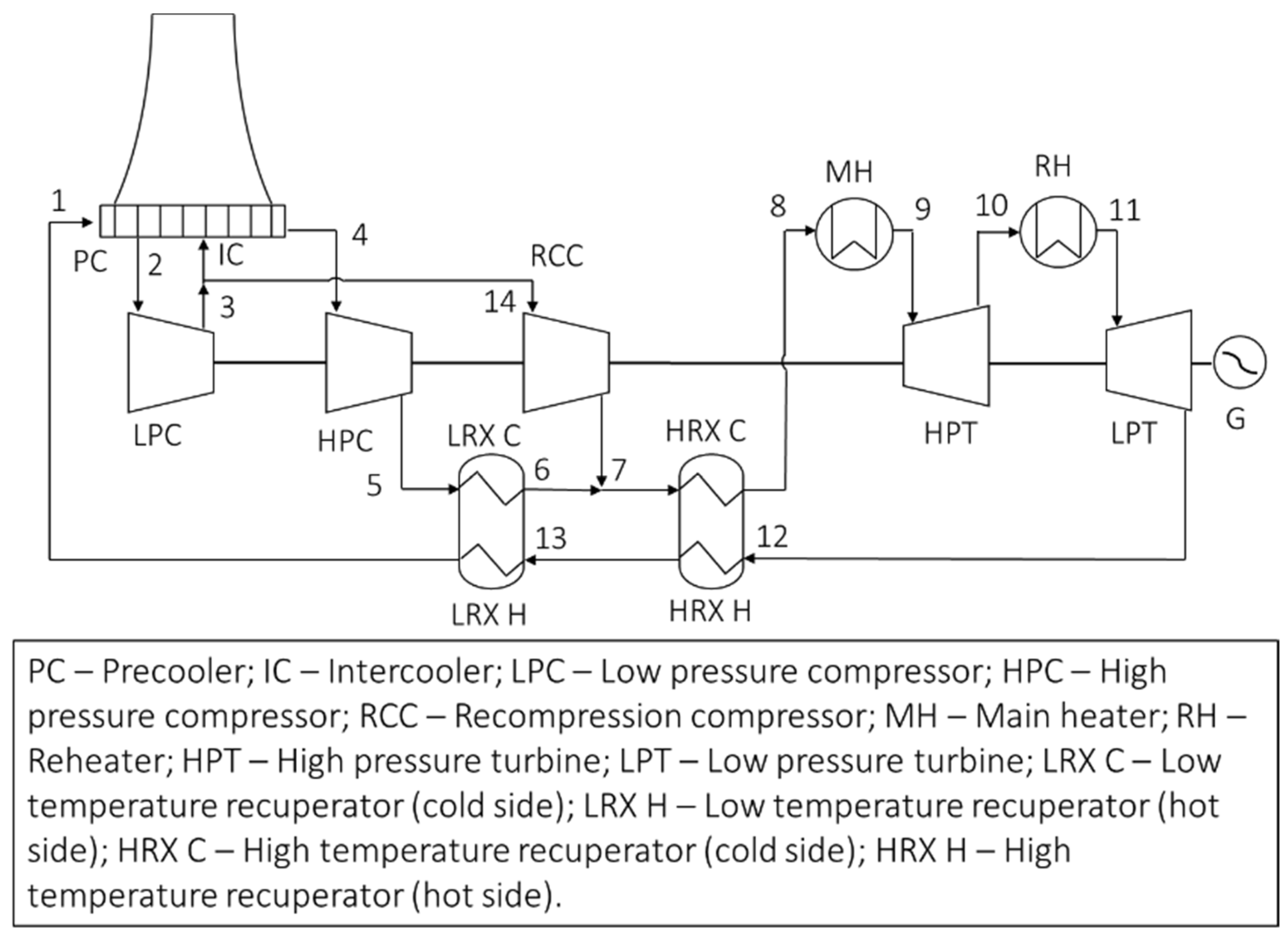
Figure 2.
Example of the front view of the cooling tower (a), side-on view of a single heat exchanger tube bank (b), single heat exchanger element with 8 sCO2-side passes (c). Adopted from [12].
Figure 2.
Example of the front view of the cooling tower (a), side-on view of a single heat exchanger tube bank (b), single heat exchanger element with 8 sCO2-side passes (c). Adopted from [12].
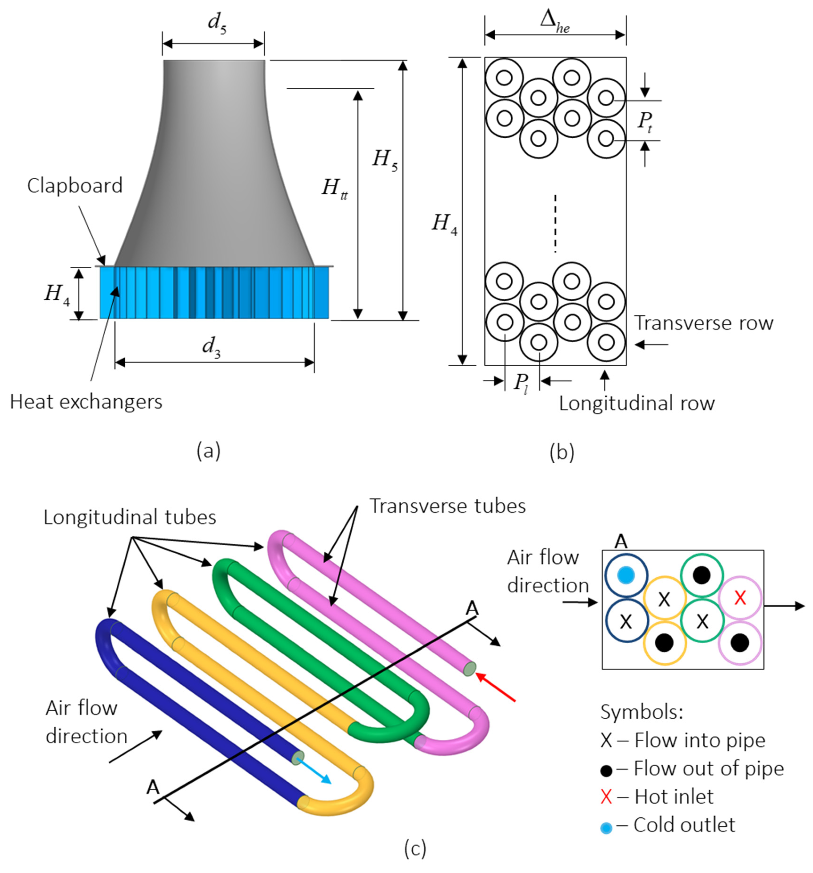
Figure 3.
Single sCO2-side heat exchanger element.
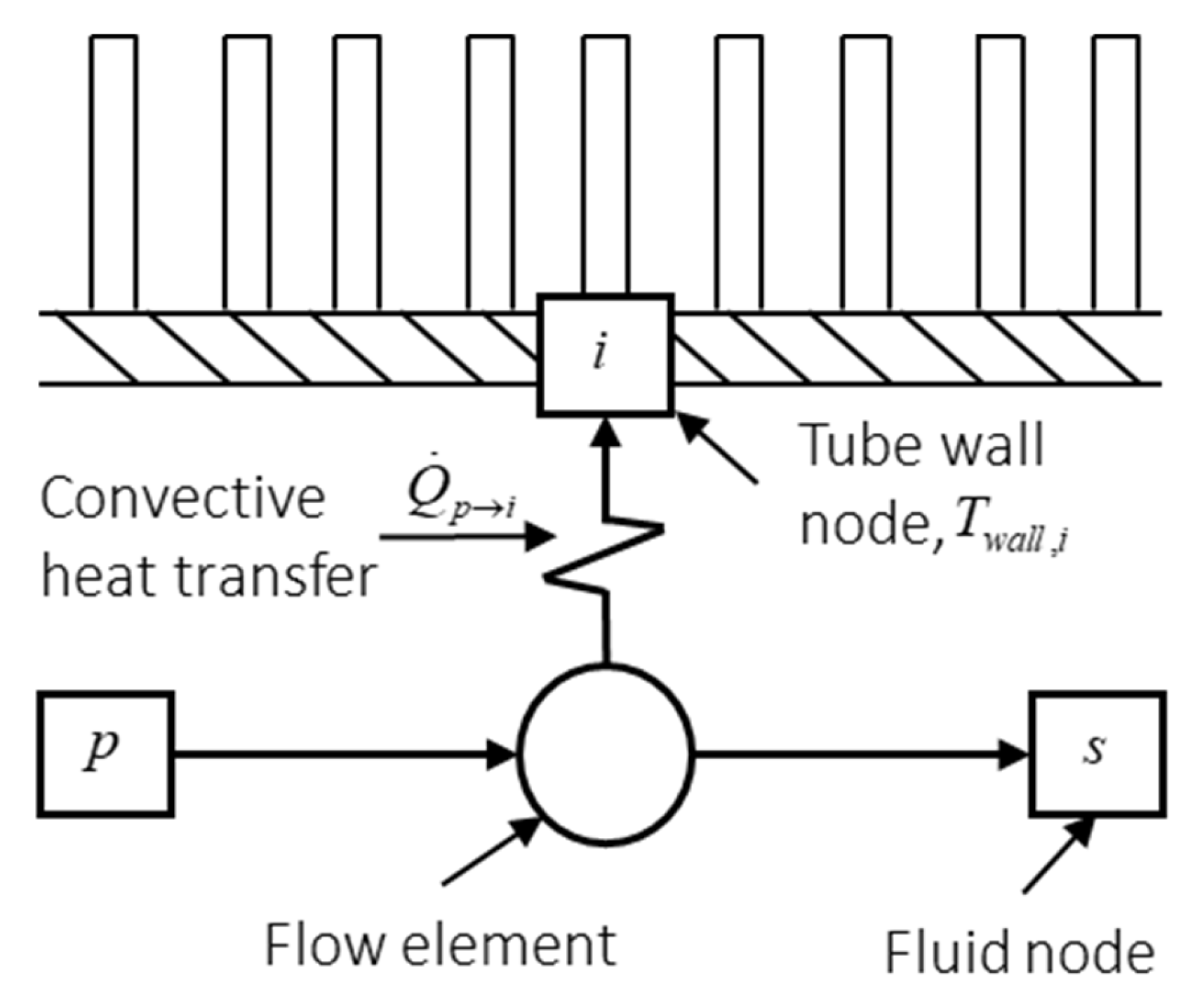
Figure 4.
Co-simulation model solution procedure flow diagram.
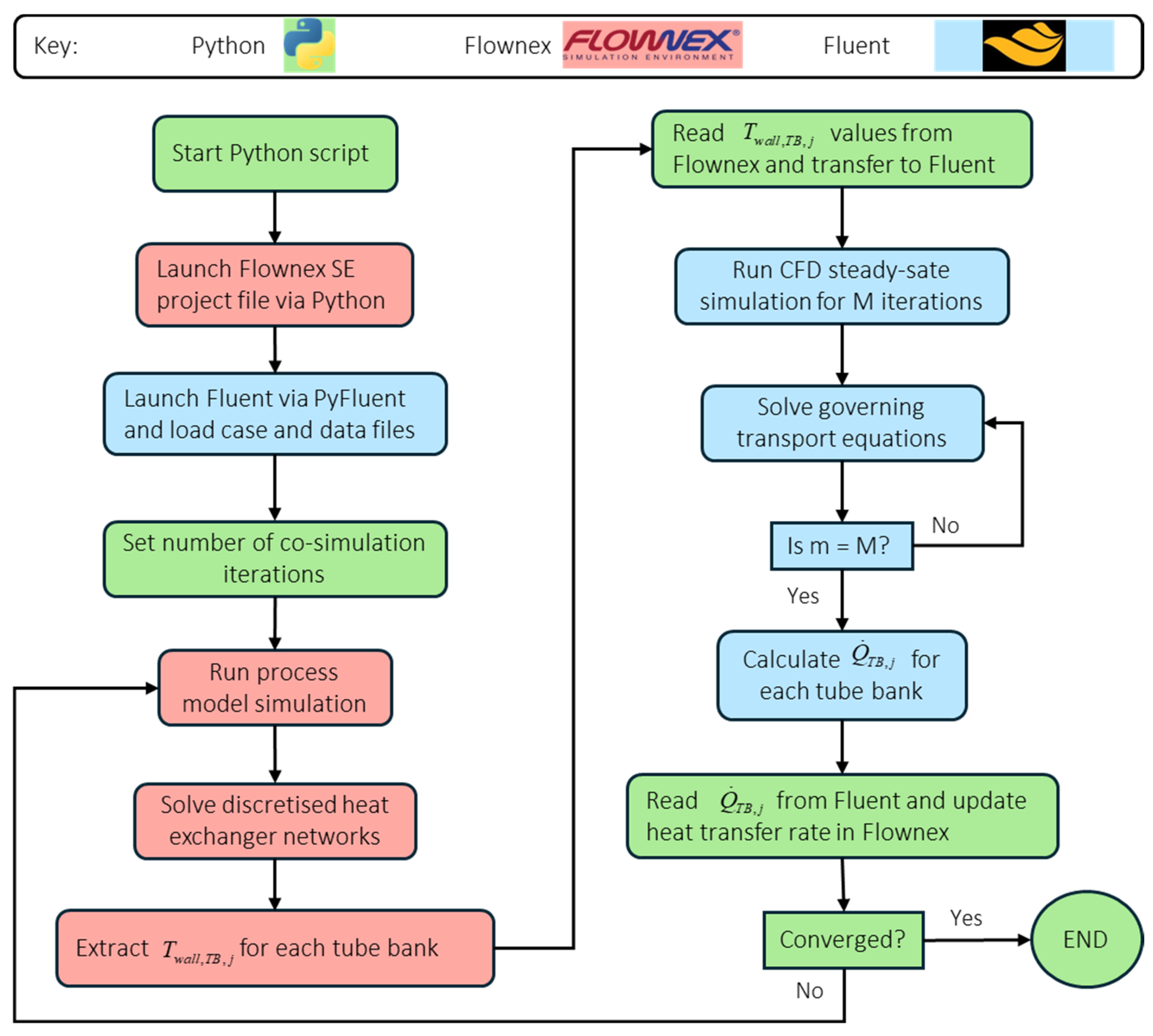
Figure 5.
Discretisation of process model heat exchanger network.
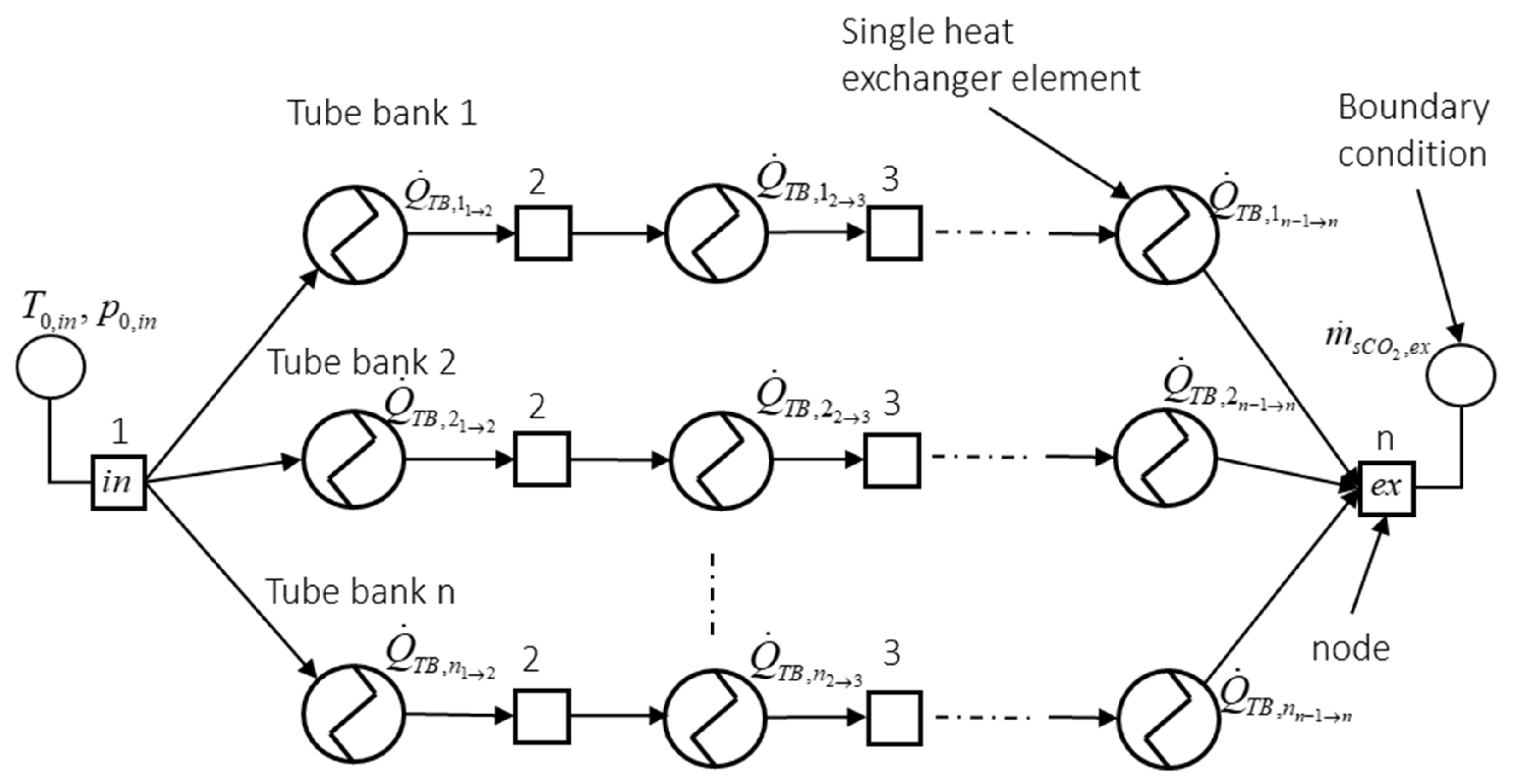
Figure 6.
Boundary condition placements and definitions of computational domain (a), lumped and alternating heat exchanger geometry options.
Figure 6.
Boundary condition placements and definitions of computational domain (a), lumped and alternating heat exchanger geometry options.
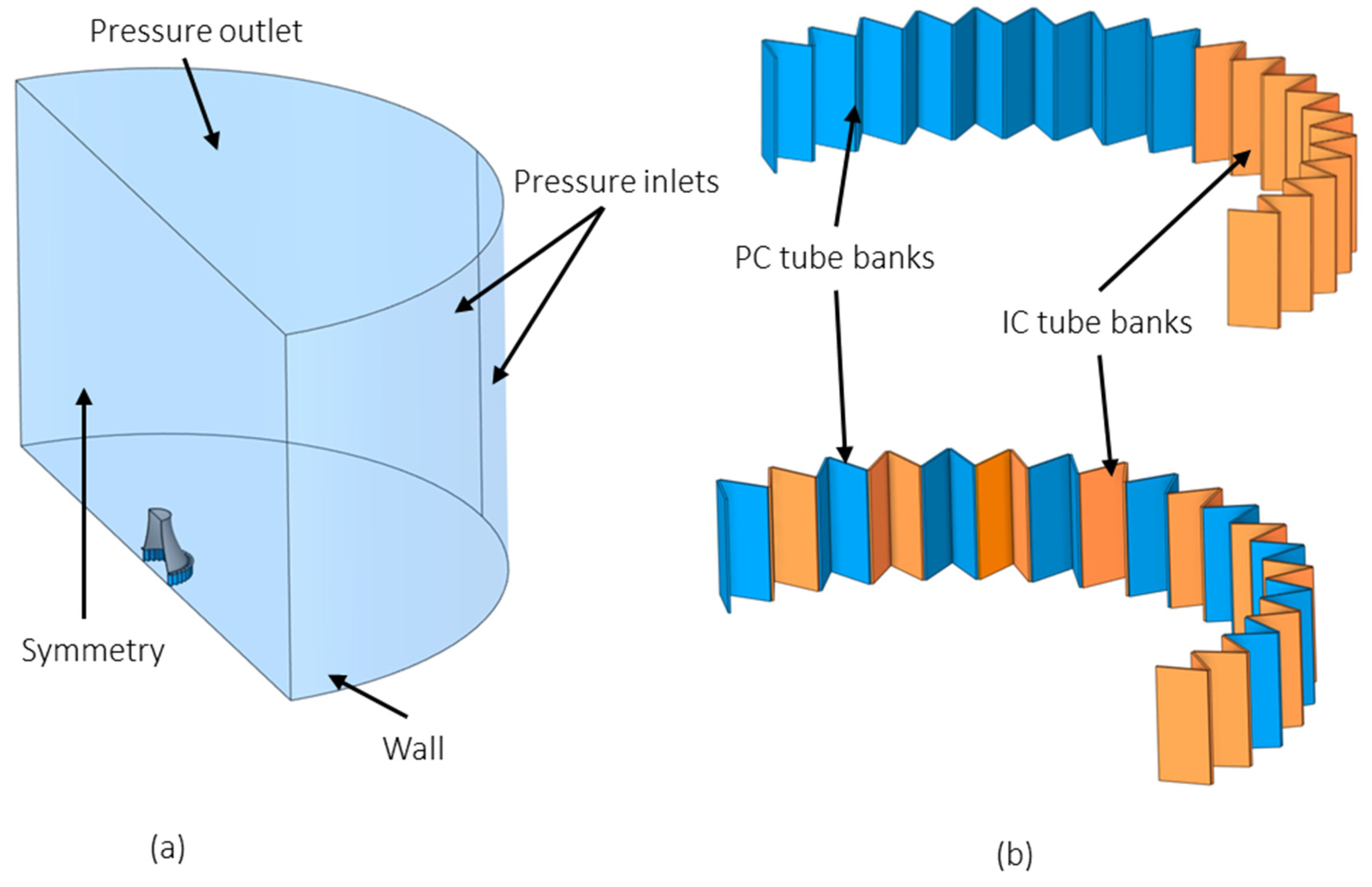
Figure 7.
Recirculation of air in front of heat exchanger (a), velocity contour of half the tower domain (b), resulting temperatures on heat exchanger surfaces from recirculation (c).
Figure 7.
Recirculation of air in front of heat exchanger (a), velocity contour of half the tower domain (b), resulting temperatures on heat exchanger surfaces from recirculation (c).
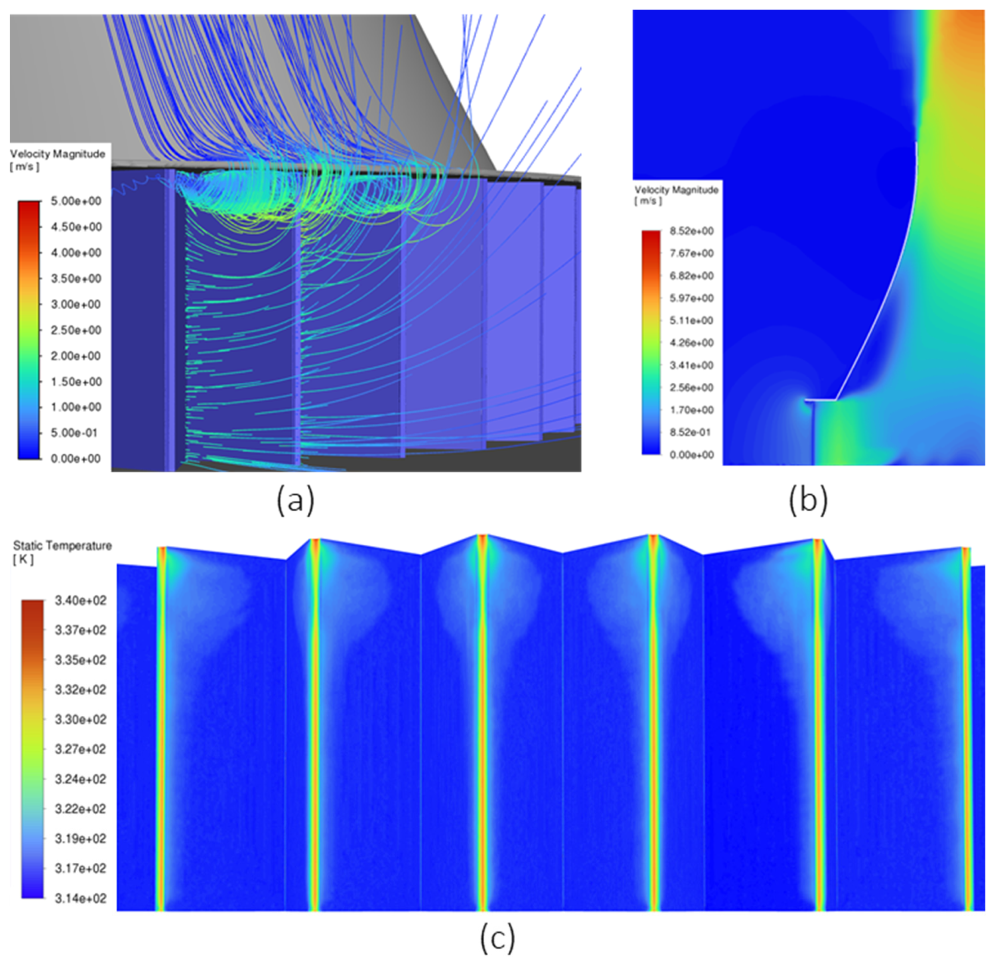
Figure 8.
Relative performance of the lumped and alternating geometries.
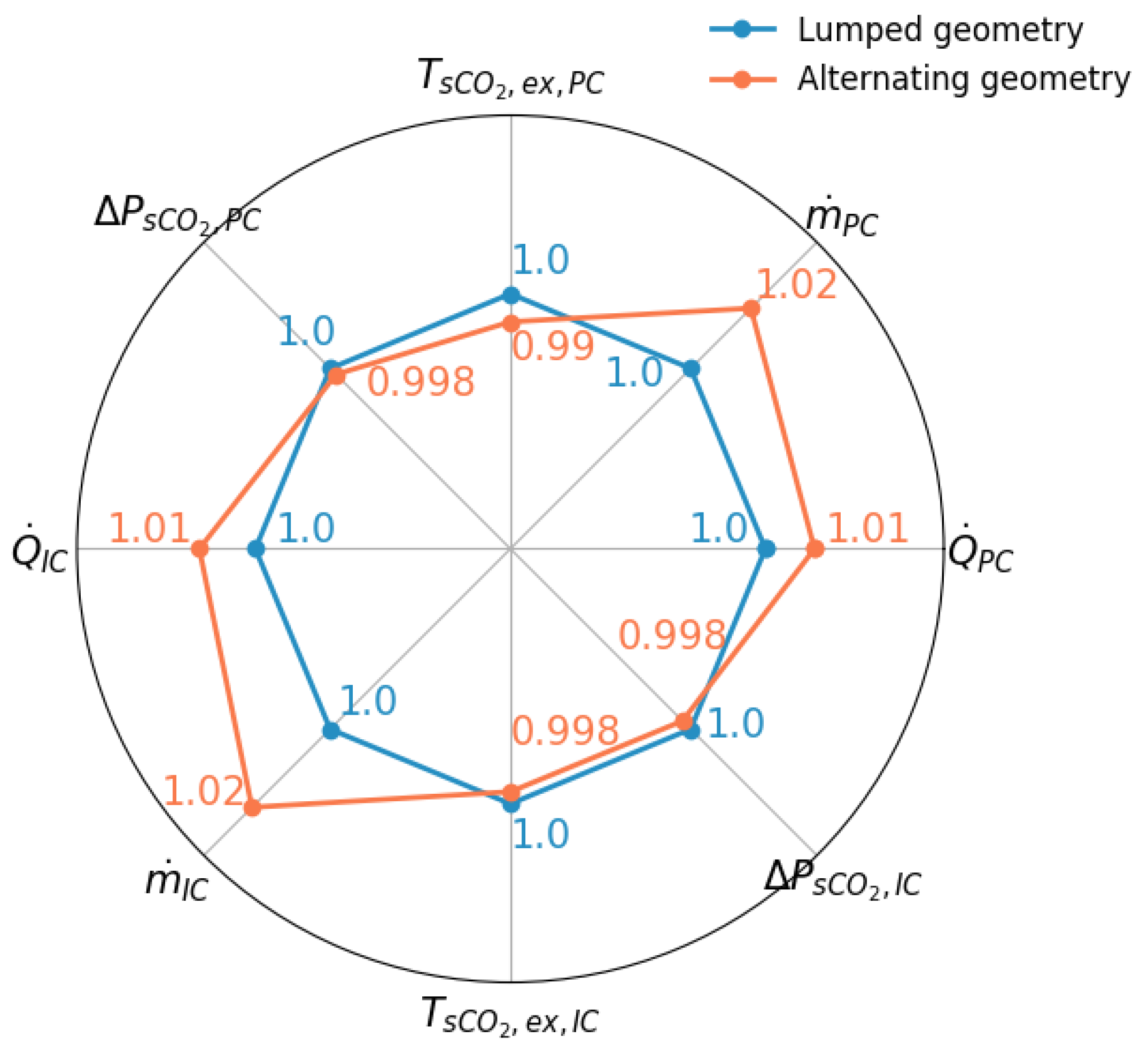
Figure 9.
Temperature and velocity contour plots of the lumped- (a,c) and alternating geometry (b,d). Tower outlet temperature and velocity plots of the lumped- (e,g) and alternating geometry (f,h).
Figure 9.
Temperature and velocity contour plots of the lumped- (a,c) and alternating geometry (b,d). Tower outlet temperature and velocity plots of the lumped- (e,g) and alternating geometry (f,h).
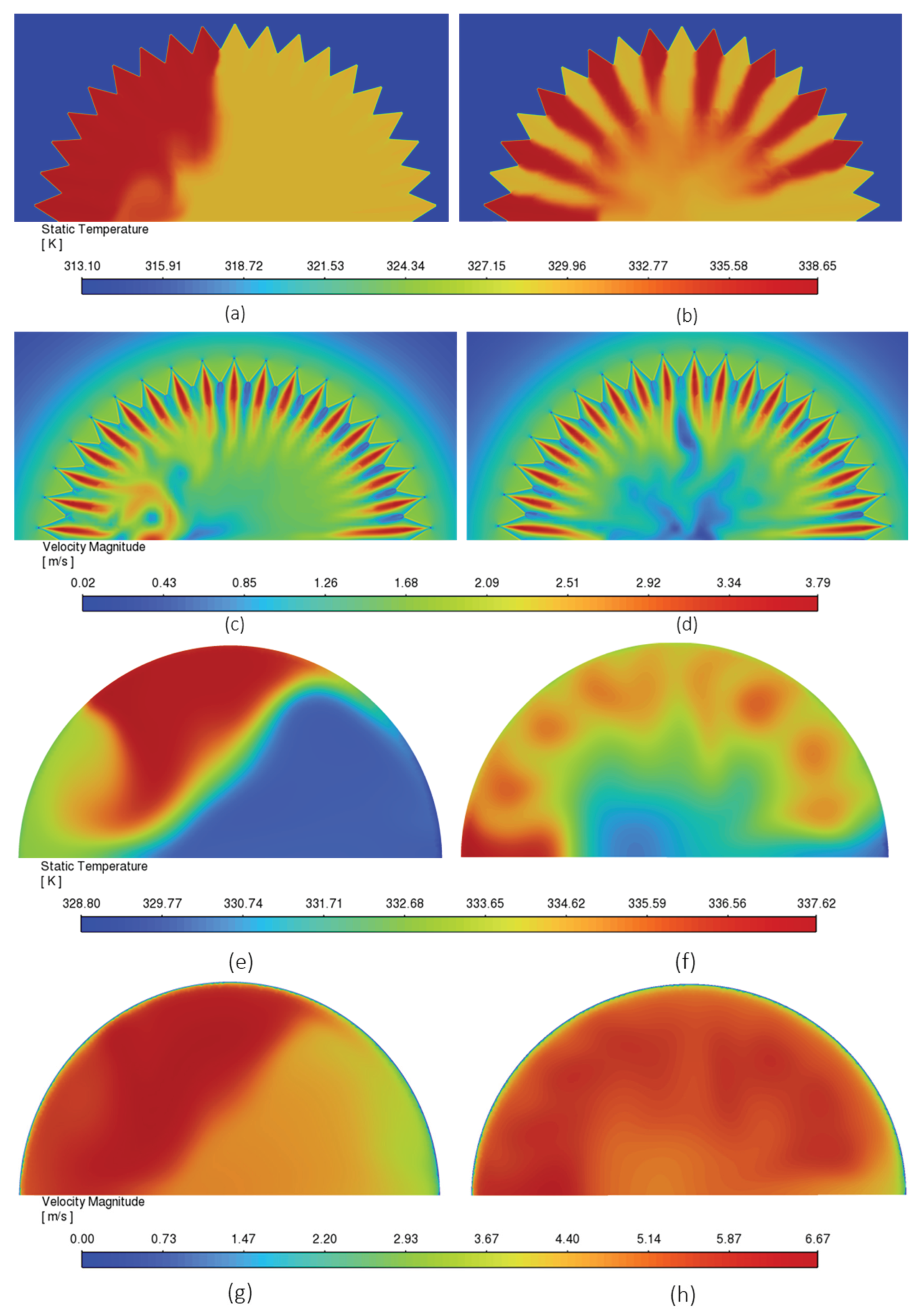

Table 1.
Air-side cooling tower dimensions.
| Parameter | Symbol | Value (m) |
|---|---|---|
| Tower height | 55.79 | |
| Heat exchanger inlet height | 11.14 | |
| Inlet diameter | 55.79 | |
| Outlet diameter | 27.89 | |
| Throat height | 50.81 |
Table 2.
Heat exchanger geometry and dimensions.
| Parameter | Symbol | Value |
|---|---|---|
| PC element passes | - | 8 |
| No. of PC tube banks | - | 35 |
| IC element passes | - | 24 |
| No. of IC tube banks | - | 41 |
| Tube material | - | Mild steel |
| Fin material | - | Aluminium |
| Tube thermal conductivity | 50 W/m∙K | |
| Fin thermal conductivity | 204 W/m∙K | |
| Transverse pitch | 58 mm | |
| Longitudinal pitch | 50.22 mm | |
| Inner tube diameter | 21.6 mm | |
| Outer tube diameter | 25.4 mm | |
| Fin outer diameter | 57.2 mm | |
| Fin root diameter | 27.6 mm | |
| Mean fin thickness | 0.5 mm | |
| Fin pitch | 2.8 mm | |
| Air flow depth | 207.86 mm |
Table 3.
sCO2-side boundary conditions.
| Parameter | PC | IC | Units |
|---|---|---|---|
| Inlet stagnation temperature | 95.35 | 72.75 | °C |
| Inlet stagnation pressure | 7.35 | 10.34 | MPa |
| Total design point mass flow rate | 275.5 | 179.1 | kg/s |
Table 4.
GCI results.
| Parameter | Mass flow rate (%) | Heat transfer rate (%) |
|---|---|---|
| Coarse to medium mesh (21) | ||
| 0.548 | 0.426 | |
| 0.682 | 0.53 | |
| Medium to fine mesh (32) | ||
| 0.264 | 0.181 | |
| 0.33 | 0.226 |
Table 5.
Comparison between discretised 1-D model from [12] and co-simulation model.
Table 5.
Comparison between discretised 1-D model from [12] and co-simulation model.
| Parameter | Discretised 1-D model | Co-simulation model | % Difference |
|---|---|---|---|
| Overall | |||
| Heat rejection rate (MW) | 81.24 | 71.35 | 13.85 |
| Air mass flow rate (kg/s) | 3671 | 3455 | 6.25 |
| Driving potential (Pa) | 36.42 | 35.75 | 1.87 |
| Precooler | |||
| Heat rejection rate (MW) | 43.72 | 40.12 | 8.97 |
| Air mass flow rate (kg/s) | 1684 | 1583 | 6.35 |
| sCO2 pressure drop (kPa) | 13.53 | 14.59 | -7.25 |
| sCO2 outlet temperature (°C) | 45.89 | 48.88 | -6.12 |
| Intercooler | |||
| Heat rejection rate (MW) | 37.52 | 31.23 | 20.13 |
| Air mass flow rate (kg/s) | 1987 | 1871 | 6.17 |
| sCO2 pressure drop (kPa) | 50.09 | 54.54 | -8.16 |
| sCO2 outlet temperature (°C) | 46.09 | 48.5 | -4.97 |
Table 6.
Overall performance comparison between lumped and alternating geometries.
| Parameter | Lumped geometry | Alternating geometry | % Difference |
|---|---|---|---|
| Heat rejection rate (MW) | 71.35 | 72.08 | 1.02 |
| Air mass flow rate (kg/s) | 3455 | 3520 | 1.88 |
| Driving potential (Pa) | 35.75 | 36.52 | 1.3 |
Disclaimer/Publisher’s Note: The statements, opinions and data contained in all publications are solely those of the individual author(s) and contributor(s) and not of MDPI and/or the editor(s). MDPI and/or the editor(s) disclaim responsibility for any injury to people or property resulting from any ideas, methods, instructions or products referred to in the content. |
© 2025 by the authors. Licensee MDPI, Basel, Switzerland. This article is an open access article distributed under the terms and conditions of the Creative Commons Attribution (CC BY) license (http://creativecommons.org/licenses/by/4.0/).
Copyright: This open access article is published under a Creative Commons CC BY 4.0 license, which permit the free download, distribution, and reuse, provided that the author and preprint are cited in any reuse.


