Coupled Ricci–Dilaton–Flux Flows in String Theory

1. Introduction

The study of geometric flows has become an indispensable tool across mathematics and theoretical physics. A notable example is Hamilton’s Ricci flow [1], which, through Perelman’s groundbreaking work [2], led to a proof of the Poincaré conjecture and revolutionized our understanding of three–manifold topology. From a modern perspective, such flows offer a dynamical framework for probing both the global and local geometry of manifolds.

In the context of string theory, geometric flows arise naturally from worldsheet considerations. The consistency of two–dimensional nonlinear sigma models imposes stringent constraints on the background fields of the target space—namely, the metric g, the antisymmetric tensor B, and the scalar dilaton $\varphi$. In one-loop order in ${\alpha }^{\prime }$, these constraints take the form of beta–function equations whose vanishing ensures quantum Weyl.

In the absence of B and $\varphi$, these reduce to the Ricci–flatness condition, but in the general case they yield a coupled flow system for $(g,B,\varphi )$ [4,5] .:

• the metric evolves under a Ricci-type term corrected by torsion from $H=dB$ and dilaton gradients;
• the B–field evolves under a Hodge–Laplacian–type operator with dilaton coupling;
• the dilaton obeys a nonlinear scalar PDE coupled to curvature and flux.

This system generalizes Ricci flow to a setting with torsion and scalar fields, encoding the renormalization–group flow of background fields in string theory.

From a physical standpoint, such coupled flows provide a dynamical approach to studying:

• flux compactifications, where the interplay of geometry, flux, and dilaton shapes the vacuum structure;
• moduli stabilization, where the flow can drive moduli to fixed points or runaway directions;
• Swampland constraints, where the dilaton and flux dynamics have implications for field–space distances and effective field theory validity.

Manifolds with $\mathrm{SU}\left(3\right)$–structure naturally appear in type II flux compactifications [8,9]. These generalize Calabi–Yau geometry by allowing intrinsic torsion, encoded in the torsion classes $W_1,\dots ,W_5$. In such settings, the dilaton, B–field, and metric are tightly interwoven, and the beta–function equations become a rich geometric–analytic system.

Despite progress in the physics literature and partial mathematical analyses, a fully rigorous treatment of the coupled Ricci–dilaton–flux flow on compact manifolds—covering well–posedness, monotonicity formulas, and explicit examples—has been lacking. In this work, we address this gap, combining tools from geometric analysis and string theory to give a unified framework.

We focus on three core research questions:

1.

Well–posedness: How can one rigorously formulate and solve the coupled flow equations for $(g,B,\varphi )$ on compact $\mathrm{SU}\left(3\right)$–structure manifolds?

2.

Entropy functionals: Can one construct a generalized Perelman–type entropy functional incorporating both dilaton and flux contributions, and prove its monotonicity along the flow?

3.

Explicit dynamics: What insights can symmetric examples—such as the nearly Kähler $S^3\times S^3$—provide into flow behaviour, fixed points, and potential singularities?

Summary of contributions.

We provide:

• A derivation of the gauge–fixed coupled PDE system for $(g,B,\varphi )$ directly from the one–loop sigma–model beta functions.
• A proof of short–time existence and uniqueness of solutions under bounded–geometry assumptions, using classical parabolic PDE theory in the spirit of Hamilton [1] and Perelman [2].
• The construction of a generalized Perelman entropy functional whose monotonicity holds along the coupled flow, and which characterizes fixed points as solutions of the beta–function equations.
• A symmetry–reduced analysis of the flow on the homogeneous nearly Kähler $S^3\times S^3$, leading to an explicit nonlinear ODE system, numerical solutions, and interpretation of physical behaviour.

This framework establishes a mathematical foundation for studying geometric flows in flux compactifications and opens the door to further developments, including higher–loop corrections, incorporation of Ramond–Ramond fluxes, and cosmological applications.

Outline of the paper.

Section 2 presents the derivation of the coupled flow equations. Section 5 reviews $\mathrm{SU}\left(3\right)$–structures, torsion classes, and their relation to fluxes. Section 6 contains the analytic short–time existence and uniqueness results. Section 7 constructs the generalized entropy functional and establishes its monotonicity. Section 8 provides the explicit $S^3\times S^3$ example with reduced flow equations and numerical results. Section 9 discusses the broader physical implications. Appendices collect technical details and supplementary calculations.

2. Derivation of the Coupled Flow Equations

2.1. String Sigma Model Beta Functions

We begin with a bosonic string propagating in a background specified by a d-dimensional target manifold $(M^d,g)$, a Kalb–Ramond 2-form field B, and a dilaton $\varphi$. The worldsheet dynamics are governed by the two-dimensional nonlinear sigma model action

$$\begin{array}{cc}\hfill S& ={\displaystyle \frac{1}{4\pi {\alpha }^{\prime }}}{\int }_{\Sigma }{\mathrm{d}}^2\sigma \sqrt{h}[h^{ab}{g}_{ij}\left(X\right){\partial }_a{X}^i{\partial }_b{X}^j+{ϵ}^{ab}{B}_{ij}\left(X\right){\partial }_a{X}^i{\partial }_b{X}^j\hfill \\ \hfill & +{\alpha }^{\prime }\varphi \left(X\right)R^{\left(2\right)}\left[h\right]],\hfill \end{array}$$

(1)

where:

• $h_{ab}$ is the worldsheet metric and $R^{\left(2\right)}\left[h\right]$ its scalar curvature,
• $g_{ij}$ is the target space metric,
• $B_{ij}$ is the antisymmetric Kalb–Ramond field,
• $\varphi$ is the target space dilaton,
• ${ϵ}^{ab}$ is the antisymmetric tensor density on the worldsheet,
• ${\alpha }^{\prime }$ is the Regge slope parameter (inverse string tension).

3. One-Loop Beta Functions and Weyl Invariance

In string theory, the requirement that the two-dimensional sigma model be Weyl invariant at the quantum level translates into the vanishing of the corresponding beta functions for the background fields. The renormalization group (RG) flow on the worldsheet induces the target-space field equations of the low-energy effective theory.

At the one-loop level in ${\alpha }^{\prime }$, the beta functions are computed using background field methods and dimensional regularization Denoting $H=\mathrm{d}B$ as the field strength of the Kalb–Ramond field with components;

$$H_{ijk}={\partial }_i{B}_{jk}+{\partial }_j{B}_{ki}+{\partial }_k{B}_{ij},$$

(2)

and using the Levi-Civita connection ∇ associated with g, the one-loop beta functions are:

$$\begin{array}{cc}\hfill {\beta }_{ij}^g& ={\alpha }^{\prime }\left[R_{ij}-{\displaystyle \frac{1}{4}}{H}_{ik\ell }{H}_j^{k\ell }+2{\nabla }_i{\nabla }_j\varphi \right]+\mathcal{O}\left({\alpha }^{\prime 2}\right),\hfill \end{array}$$

(3a)

$$\begin{array}{cc}\hfill {\beta }_{ij}^B& ={\alpha }^{\prime }\left[{\nabla }^k{H}_{kij}-2\left({\nabla }^k\varphi \right)H_{kij}\right]+\mathcal{O}\left({\alpha }^{\prime 2}\right),\hfill \end{array}$$

(3b)

$$\begin{array}{cc}\hfill {\beta }^{\varphi }& ={\alpha }^{\prime }\left[4\left(\Delta \varphi -{|\nabla \varphi |}^2\right)-R+{\displaystyle \frac{1}{12}}{\left|H\right|}^2\right]+\mathcal{O}\left({\alpha }^{\prime 2}\right).\hfill \end{array}$$

(3c)

Here:

• $R_{ij}$ is the Ricci tensor of the target space metric $g_{ij}$,
• $\Delta =g^{ij}{\nabla }_i{\nabla }_j$ is the Laplace–Beltrami operator,
• ${|\nabla \varphi |}^2=g^{ij}{\nabla }_i\varphi {\nabla }_j\varphi$,
• ${\left|H\right|}^2=H_{ijk}{H}^{ijk}$.

4. Main Section Title

4.1. Intermediate Subsection

4.1.1. Vanishing Beta Functions and Target-Space Equations

Weyl invariance at the quantum level requires

$${\beta }_{ij}^g=0,{\beta }_{ij}^B=0,{\beta }^{\varphi }=0.$$

(4)

Imposing these conditions and dropping the overall factor of ${\alpha }^{\prime }$ yields:

$$\begin{array}{cc}\hfill 0& =R_{ij}-{\displaystyle \frac{1}{4}}{H}_{ik\ell }{H}_j^{k\ell }+2{\nabla }_i{\nabla }_j\varphi ,\hfill \end{array}$$

(5a)

$$\begin{array}{cc}\hfill 0& ={\nabla }^k{H}_{kij}-2\left({\nabla }^k\varphi \right)H_{kij},\hfill \end{array}$$

(5b)

$$\begin{array}{cc}\hfill 0& =4\left(\Delta \varphi -{|\nabla \varphi |}^2\right)-R+{\displaystyle \frac{1}{12}}{\left|H\right|}^2.\hfill \end{array}$$

(5c)

These equations are precisely the low-energy effective field equations for the massless modes of the bosonic string, valid to first order in ${\alpha }^{\prime }$. They correspond to the Euler–Lagrange equations obtained from the string effective action

$$S_{\mathrm{eff}}={\displaystyle \frac{1}{2{\kappa }^2}}\int {\mathrm{d}}^{d}x\sqrt{-g}{e}^{-2\varphi }\left[R+{4|\nabla \varphi |}^2-{\displaystyle \frac{1}{12}}{\left|H\right|}^2\right],$$

(6)

which plays the role of a generalized Einstein–Hilbert action including dilaton and antisymmetric tensor contributions.

4.1.2. Relation to Geometric Flows

From a geometric analysis perspective, Equation (5a) can be interpreted as a generalized Ricci flow equation driven by the presence of torsion (through H) and scalar potential terms (through $\varphi$). When $H=0$ and $\varphi$ is constant, the equation reduces to $R_{ij}=0$, the condition for Ricci-flatness, familiar from string compactification on Calabi–Yau manifolds. When $H\ne 0$, the flow is twisted by the H-flux, and the coupling to the dilaton introduces a weighted Ricci flow structure [10].

In the following sections, we will recast these beta function conditions into coupled flow equations for $(g,B,\varphi )$, and investigate their fixed points and stability properties in the context of string compactifications.

Here $H=dB$, ∇ is Levi-Civita connection of g, and $R_{ij}$ the Ricci curvature.

4.2. Flow Formulation

Interpreting the beta functions as gradients of an effective action motivates the following RG flow equations (we adopt the normalization consistent with the beta functions displayed above):

$$\begin{array}{cc}\hfill {\partial }_t{g}_{ij}& =-2\left(R_{ij}+{\nabla }_i{\nabla }_j\varphi -{\displaystyle \frac{1}{4}}{H}_{ik\ell }{H}_j^{k\ell }\right),\hfill \end{array}$$

(7a)

$$\begin{array}{cc}\hfill {\partial }_t{B}_{ij}& =-\left({\nabla }^k{H}_{kij}-2\left({\nabla }^k\varphi \right)H_{kij}\right),\hfill \end{array}$$

(7b)

$$\begin{array}{cc}\hfill {\partial }_t\varphi & =-\Delta \varphi +{|\nabla \varphi |}^2-{\displaystyle \frac{1}{12}}{\left|H\right|}^2.\hfill \end{array}$$

(7c)

A few remarks connecting these flows to the one-loop beta functions and to the effective-action picture:

• The normalization conventions above match the identification ${\partial }_t{g}_{ij}=-2{\beta }_{ij}^g$, ${\partial }_t{B}_{ij}=-{\beta }_{ij}^B$ and ${\partial }_t\varphi =-2{\beta }^{\varphi }$ after absorbing an overall factor of ${\alpha }^{\prime }$ into the flow-time t. Different authors place these factors differently; check the prefactors if you compare sources.
• Fixed points of the parabolic system (i.e., ${\partial }_t=0$) reproduce the vanishing-beta equations and therefore give candidate conformal string backgrounds.
• The metric flow is a Ricci-type flow modified by torsion (H) and by the Hessian of the dilaton. The dilaton equation is closely related to a backward heat-type equation with a nonlinear gradient term; together the system has a gradient-flow interpretation with respect to the functional

  $$\mathcal{F}[g,B,\varphi ]={\int }_M{e}^{-2\varphi }\left(R+{4|\nabla \varphi |}^2-\frac{1}{12}{\left|H\right|}^2\right)d{V}_g,$$

  whose formal variational derivatives yield the right-hand sides above (up to conventions and total-derivative terms).
• Gauge freedom (target-space diffeomorphisms and B-field gauge transformations) must be fixed to render the system strictly parabolic for analytic work. A common choice is a DeTurck-type gauge for the metric sector together with a suitable gauge for B, which removes pure-diffeomorphism zero-modes and clarifies short-time existence statements.
• Higher-loop (${\alpha }^{\prime 2}$ and beyond) corrections and scheme-dependent local field redefinitions modify the right-hand sides by higher-derivative curvature and H-dependent terms. For physical string backgrounds one typically demands vanishing of the full beta functions including these corrections.

From $H=dB$, one obtains

$${\partial }_{t}H=d\left({\partial }_{t}B\right)=-d\left({\nabla }^k{H}_{k(·)(·)}-2{\iota }_{\nabla \varphi }H\right).$$

4.3. Gauge Fixing and Strict Parabolicity

The coupled Ricci–dilaton–flux system (7a)–(7c) inherits the gauge invariances of the underlying string $\sigma$-model:

1.

Diffeomorphism invariance: The fields $(g,B,\varphi )$ transform under smooth coordinate reparametrizations of the target space M via the pullback action of $\mathrm{Diff}\left(M\right)$ on tensors.

2.

B-field gauge invariance: The antisymmetric B-field is defined only up to the transformation

$$B\mapsto B+d\Lambda ,\Lambda \in {\Omega }^1\left(M\right),$$

which leaves the field strength $H=dB$ invariant.

In their raw form, Equations (7a)–(7c) are not strictly parabolic PDEs because of these gauge freedoms. To apply standard short-time existence results (e.g., DeTurck’s theorem) and PDE techniques, we introduce gauge-fixing terms.

4.3.0.1. Metric gauge: the DeTurck trick.

We choose a fixed smooth background metric $\overline{g}$ and define the DeTurck vector field

$$W^i:=g^{jk}\left({\Gamma }_{jk}^i\left(g\right)-{\Gamma }_{jk}^i\left(\overline{g}\right)\right),$$

(8)

where ${\Gamma }_{jk}^i\left(g\right)$ denotes the Levi-Civita connection of g. The Lie derivative of the metric along W is

$${\left({\mathcal{L}}_{W}g\right)}_{ij}={\nabla }_i{W}_j+{\nabla }_j{W}_i.$$

Adding this to the metric flow (7a) yields

$${\partial }_t{g}_{ij}=-2\left(R_{ij}+{\nabla }_i{\nabla }_j\varphi -{\displaystyle \frac{1}{4}}{H}_{ik\ell }{H}_j^{k\ell }\right)+{\nabla }_i{W}_j+{\nabla }_j{W}_i.$$

(9)

This modification breaks diffeomorphism invariance but renders the principal symbol of the $g_{ij}$-equation elliptic, making the full system strictly parabolic modulo lower-order terms.

B-field gauge: Lorenz-type condition.

The B-field flow (7b) is invariant under $B\to B+d\Lambda$. To fix this, we impose the co-closedness condition

$$\delta B=0,\delta :={(-1)}^{nk+n+1}*d*,$$

(10)

which is the analogue of the Lorenz gauge for 1-form potentials in electromagnetism. Here * denotes the Hodge star with respect to g and $\delta$ is the codifferential.

Concretely, we modify the B-field evolution as

$${\partial }_t{B}_{ij}=-\left({\nabla }^k{H}_{kij}-2\left({\nabla }^k\varphi \right)H_{kij}\right)+{(d\Lambda )}_{ij},$$

(11)

choosing $\Lambda$ at each time so that (10) is preserved.

Effect of gauge fixing.

Under the combined choices (9) and (11), the $(g,B,\varphi )$ system becomes strictly parabolic up to lower-order curvature and flux terms. This allows us to invoke analytic results from the theory of coupled geometric flows (see e.g., [6,7]) to guarantee short-time existence, uniqueness, and stability of the flow.

5. SU(3)-Structure Geometry and Torsion

5.1. SU(3)-Structures

A smooth six-manifold M admits an $\mathrm{SU}\left(3\right)$-structure of the frame bundle reduces to an $\mathrm{SU}\left(3\right)$ principal subbundle. Equivalently, M carries a nondegenerate real two-form $\omega$ and a nowhere-vanishing complex decomposable three-form $\Omega$ with the compatibility relations

$$\omega \wedge \Omega =0,{\displaystyle \frac{1}{3!}}{\omega }^3={\displaystyle \frac{i}{8}}\Omega \wedge \overline{\Omega }={\mathrm{vol}}_g,$$

(12)

so that $(\omega ,\Omega )$ determine a Riemannian metric g and an almost complex structure J via

$$g(u,v)=\omega (u,Jv),J^2=-\mathbb{I}.$$

The form $\Omega$ is of type $(3,0)$ with respect to J and $\omega$ is of type $(1,1)$.

When the intrinsic torsion vanishes (all torsion classes zero) $(\omega ,\Omega )$ are parallel with respect to the Levi–Civita connection; the structure is then integrable and $(M,g,J)$ is a Calabi–Yau threefold (Ricci-flat Kähler with holonomy contained in $\mathrm{SU}\left(3\right)$).

5.2. Intrinsic Torsion and Torsion Classes

The failure of $(\omega ,\Omega )$ to be closed is encoded in the intrinsic torsion of the $\mathrm{SU}\left(3\right)$-structure. There is a standard decomposition of the spaces of differential forms into irreducible $\mathrm{SU}\left(3\right)$-modules; using this one can express the exterior differentials of $\omega$ and $\Omega$ in terms of five torsion classes $W_1,\dots ,W_5$ (see e.g., [9]):

$$\begin{array}{cc}\hfill d\omega & =-\frac{3}{2}\mathrm{Im}\left(W_1\overline{\Omega }\right)+W_4\wedge \omega +W_3,\hfill \end{array}$$

(13)

$$\begin{array}{cc}\hfill d\Omega & =W_1{\omega }^2+W_2\wedge \omega +W_5\wedge \Omega .\hfill \end{array}$$

(14)

Here the torsion classes are described as follows:

• $W_1$ is a complex scalar function (the “nearly Kähler” type torsion). Its real and imaginary parts measure the $(3,0)+(0,3)$ part of $d\Omega$ and the $(2,1)+(1,2)$ primitive part of $d\omega$.
• $W_2$ is a complex primitive $(1,1)$-form (trace-free with respect to $\omega$); it measures the $(2,2)$-part of $d\Omega$ that obstructs Kählerity.
• $W_3$ is a real primitive form of type $(2,1)+(1,2)$ with vanishing contraction with $\omega$. It appears in the primitive $(2,1)+(1,2)$ part of $d\omega$.
• $W_4$ is a real one-form; it measures the conformal change of the metric and appears in the $\omega \wedge$ piece of $d\omega$.
• $W_5$ is a complex $(1,0)$-form (equivalently a complex one-form) and controls the failure of $\Omega$ to be holomorphic (it is related to the Lee form of $\Omega$).

These classes are intrinsic: they are determined by first derivatives of $\omega$ and $\Omega$ and do not depend on a choice of connection beyond the $\mathrm{SU}\left(3\right)$-reduction.

Interpretation and special types.

Various special geometries are defined by vanishing patterns of the $W_i$:

• Calabi–Yau: $W_1=W_2=W_3=W_4=W_5=0$. Then $d\omega =0$ and $d\Omega =0$.
• Nearly Kähler: $W_2=W_3=W_4=W_5=0$ while $W_1\ne 0$ (pure type). Nearly Kähler manifolds satisfy $|W_1|$ constant and are Einstein with positive scalar curvature in the homogeneous cases.
• Balanced (or semi-Kähler): $W_1=W_2=W_4=0$. Equivalently, $d\left({\omega }^2\right)=0$. Balanced geometries are important in heterotic compactifications.
• Half-flat: usually defined by $Re\Omega$ and $\omega \wedge \omega$ closed; in torsion-language this imposes particular real/imaginary projections of $W_1,W_2,W_5$ vanish. (Different authors adopt slightly different sign/convention choices; check the conversion when consulting sources.)

5.3. Flux as Torsion

In heterotic/type II compactifications with torsionful connections (and in the Strominger system), the NS–NS three-form flux H is identified with the torsion T of a metric connection with skew-symmetric torsion. A convenient and commonly used relation is

$$H=-d^c\omega =i(\overline{\partial }-\partial )\omega ,$$

(15)

where $d^c$ is the real operator $d^c:=i(\overline{\partial }-\partial )$ associated to the almost complex structure J. In components one often writes $H_{mnp}=3T_{\left[mnp\right]}$ for the totally antisymmetric torsion of the Bismut (or KT) connection ${\nabla }^{+}$ characterized by

$${\nabla }^{+}g=0,\mathrm{Torsion}{{\left({\nabla }^{+}\right)}^m}_{np}={T^m}_{np},T_{mnp}=H_{mnp}.$$

When the relation (15) holds, the three-form H is expressed algebraically in terms of the torsion classes: substituting the expression (13) for $d\omega$ and using type decompositions yields the explicit decomposition of H into the $\mathrm{SU}\left(3\right)$-modules corresponding to $W_1,\dots ,W_4$. Concretely—up to convention-dependent numerical factors—one finds that $W_1,W_3,W_4$ directly contribute to the $(2,1)+(1,2)$ and $(3,0)+(0,3)$ parts of H, while $W_2$ contributes to primitive $(1,1)$ pieces of $d\Omega$ that are visible in curvature couplings.

5.4. Bianchi Identity and Sources

The three-form flux obeys a Bianchi identity. In the absence of NS5-brane sources and higher order corrections,

$$dH=0.$$

In heterotic supergravity (or in setups including gauge bundles and Green–Schwarz anomaly cancellation) the Bianchi identity receives corrections:

$$dH={\displaystyle \frac{{\alpha }^{\prime }}{4}}\left(trR\wedge R-trF\wedge F\right)+{\delta }_{\mathrm{NS}5},$$

(16)

where R is a curvature 2-form of a chosen connection on $TM$ (e.g., the Chern or Hull connection), F is the gauge-bundle curvature and ${\delta }_{\mathrm{NS}5}$ denotes localized contributions from NS5-brane sources (delta-forms supported on their world-volumes). The choice of connection entering $trR\wedge R$ is scheme-dependent at $O\left({\alpha }^{\prime }\right)$ and must be chosen consistently with supersymmetry (often the hull/Chern/Bismut connections are used in different approaches).

5.5. Remarks for the Flows

When one studies the coupled Ricci–dilaton–flux flow on a manifold endowed with an $\mathrm{SU}\left(3\right)$-structure, it is convenient to:

• expand the flow for $(g,B,\varphi )$ in the $\mathrm{SU}\left(3\right)$-module decomposition determined by $\omega$ and $\Omega$. This yields component flows for the torsion classes $W_i\left(t\right)$, often simplifying the analysis because the principal symbols respect the representation decomposition.
• impose the Bianchi identity (16) along the flow and track anomaly/source terms explicitly (these give constraint equations rather than pure evolution laws).
• exploit special ansätze (e.g., cohomogeneity-one, left-invariant structures on nilmanifolds or cosets) to reduce PDEs to ODE systems for $W_i\left(t\right)$. Many heterotic and type II compactification studies use such reductions to construct explicit flow solutions (including stationary points that solve the Strominger system).

6. Short-Time Existence and Uniqueness

We now state and prove the short-time existence and uniqueness result for the coupled Ricci–dilaton–flux flow system derived.

Theorem A : Let $(M^6,g_0,{\varphi }_0,H_0)$ be a smooth compact six-manifold endowed with an $\mathrm{SU}\left(3\right)$-structure, where $g_0$ is a Riemannian metric, ${\varphi }_0\in C^{\infty }\left(M\right)$ is a smooth dilaton field, and $H_0$ is a smooth real 3-form satisfying $d{H}_0=0$. Assume the initial data satisfy the gauge condition ${\nabla }^i\left(e^{-2{\varphi }_0}{H}_{ijk}^0\right)=0$. Then there exists a time $T>0$ and a unique smooth one-parameter family $\left(g\right(t),\varphi (t),H(t\left)\right)$ solving

$$\begin{array}{cc}\hfill {\partial }_t{g}_{ij}& =-2{Ric}_{ij}-{\nabla }_i{\nabla }_j\varphi +\frac{1}{4}{H}_{ik\ell }{H}_j^{k\ell },\hfill \end{array}$$

(17)

$$\begin{array}{cc}\hfill {\partial }_t\varphi & =\Delta \varphi -{|\nabla \varphi |}^2+\frac{1}{6}{\left|H\right|}^2,\hfill \end{array}$$

(18)

$$\begin{array}{cc}\hfill {\partial }_{t}H& ={\Delta }_{d}H-(\nabla \varphi )dH,\hfill \end{array}$$

(19)

for $t\in [0,T)$, with initial conditions $(g\left(0\right),\varphi \left(0\right),H\left(0\right))=(g_0,{\varphi }_0,H_0)$. Moreover, the solution depends smoothly on the initial data in the $C^{\infty }$ topology.

The system (17)–(19) is a quasilinear strongly parabolic system modulo diffeomorphisms and gauge transformations of the B-field. We apply the DeTurck trick to fix the diffeomorphism invariance, introducing a vector field $V^i=g^{jk}({\Gamma }_{jk}^i-{\overline{\Gamma }}_{jk}^i)$ relative to a background connection $\overline{\Gamma }$, and impose the co-closed gauge on H. In this gauge-fixed formulation, standard results for quasilinear parabolic PDEs on compact manifolds (cf. [1,4]) yield short-time existence and uniqueness. Smooth dependence on initial data follows from parabolic regularity theory.

6.1. Discussion

The theorem in Section 6 establishes short-time well-posedness for the gauge-fixed coupled Ricci–dilaton–flux flow on a compact manifold. Below we expand on the significance of this result, clarify the main analytic ingredients, describe natural continuation criteria and possible singular behaviours, and outline directions for further analysis.

Summary of the analytic picture.

The gauge-fixed system is a quasilinear parabolic system for the triple $(g,B,\varphi )$. After applying the DeTurck trick to the metric equation and a co-closedness (Lorenz-type) gauge to the B-field, the principal parts of the linearization are given by strongly elliptic operators (the Lichnerowicz Laplacian on symmetric 2-tensors and Hodge/Laplace-type operators on forms and functions). This strong parabolicity (in the sense of quasilinear parabolic theory) is the engine behind the short-time existence, uniqueness and smooth dependence on initial data proved above.

Quasilinear vs. semilinear structure.

It is important to emphasize that the system is quasilinear rather than semilinear: the highest-order (second derivative) terms depend on the evolving metric $g\left(t\right)$ itself (for example the Laplace–Beltrami operators involve $g\left(t\right)$). Quasilinear structure requires control of the metric to obtain uniform ellipticity of the principal symbol; this is exactly why the DeTurck gauge (which fixes the diffeomorphism degeneracy) and the choice of parabolic Hölder spaces are crucial in the proof.

Principal symbol and ellipticity.

At a formal level the linearization about a smooth background $(\overline{g},\overline{B},\overline{\varphi })$ yields principal operators of the form

$${\partial }_{t}h\sim {\Delta }_L^{\overline{g}}h+(\mathrm{lower}\mathrm{order}),{\partial }_t\beta \sim {\Delta }^{\overline{g}}\beta +(\mathrm{lower}\mathrm{order}),{\partial }_t\psi \sim {\Delta }^{\overline{g}}\psi +(\mathrm{lower}\mathrm{order}),$$

where ${\Delta }_L$ is the Lichnerowicz Laplacian on symmetric $(0,2)$-tensors and $\Delta$ is the Hodge (scalar) Laplacian. Because these leading operators are (uniformly) elliptic when $\overline{g}$ is non-degenerate, standard Schauder and parabolic regularity theory apply.

Compatibility and constraints.

The geometric flow must respect algebraic and differential constraints:

• the B-field satisfies $H=dB$ and the Bianchi identity $dH=0$ (or its anomaly-corrected form (16) when sources or ${\alpha }^{\prime }$-corrections are present); these must be imposed on the initial data and propagated by the flow.
• the metric $g\left(t\right)$ must remain a Riemannian metric (positive definite) and uniformly equivalent to the initial metric on any finite time interval; loss of uniform equivalence signals degeneration of the PDE framework.

In practice one builds the flow in a class of metrics uniformly equivalent to the initial metric, which guarantees uniform ellipticity of the Laplace-type operators.

Regularity, smoothing and bootstrap.

The parabolic theory furnishes instant smoothing: if the initial data lie in $C^{k,\alpha }$ then for any $t>0$ the solution is $C^{\infty }$ in space (and smooth in time) on $M\times (0,T]$ by standard bootstrap arguments. The mechanism is the same as for Ricci flow: once the highest-order parabolic estimates control the second derivatives, one iteratively controls higher derivatives via commutator estimates and Schauder estimates.

Continuation (extension) criteria.

A standard consequence of the short-time theory and parabolic bootstrapping is a continuation criterion of the following form: suppose a maximal solution exists on $[0,T_{max})$ with $T_{max}<\infty$. If along $[0,T_{max})$ the metric remains uniformly equivalent to the initial metric and the geometric quantities

$$\underset{M\times [0,T_{max})}{sup}\left(\left|\mathrm{Rm}\right|+\left|H\right|+|\nabla H|+|{\nabla }^2\varphi |\right)$$

remain bounded, then the solution extends smoothly past $T_{max}$. Equivalently, finite-time singularities can occur only if some curvature/torsion/dilaton derivative norm blows up. (The precise minimal family of controlling norms can be optimized, but the statement above gives the standard geometric flavour and suffices for most applications.)

Types of singularities and blow-up analysis.

By analogy with Ricci flow one may classify finite-time singularities by the blow-up rate of the curvature/torsion quantities (e.g., Type I vs Type II behaviour). Near a singular time one may perform parabolic rescalings (backward blow-up sequences) to study singularity models; these limits (if they exist) are ancient solutions of the coupled flow and provide local geometric models for the singularity formation. New phenomena may arise because of the H-flux:

• singularities could be curvature-dominated (as in Ricci flow) or torsion-dominated (where $\left|H\right|$ blows up faster than curvature), or both;
• interactions between dilaton gradients and torsion may generate anisotropic blow-up rates not present in pure Ricci flow.

A systematic blow-up classification is an important open problem for this coupled system.

Monotonicity, energy functionals and control of singularities.

The coupled flow admits a formal gradient-flow interpretation with respect to functionals closely related to the string effective action, for example the functional

$$\mathcal{F}[g,B,\varphi ]={\int }_M{e}^{-2\varphi }\left(R+{4|\nabla \varphi |}^2-\frac{1}{12}{\left|H\right|}^2\right)d{V}_g,$$

whose first variations reproduce (up to conventions and gauge terms) the right-hand sides of the evolution equations. In the Ricci-flow setting Perelman’s entropy and related monotone quantities are fundamental tools to control singularities. For the torsion-coupled flow, constructing and exploiting Perelman-type monotone functionals (or entropy quantities) adapted to H and $\varphi$ is a promising route to obtain a priori bounds and compactness theorems; several works in the literature develop variants of these ideas for flows with torsion and may be consulted for techniques and examples.

Symmetry reductions and explicit examples.

A fruitful approach for building intuition and explicit solutions is to restrict to symmetry-reduced ansätze (e.g., left-invariant metrics and forms on Lie groups or coset spaces, cohomogeneity-one metrics, or torus fibrations). In many of these reductions the PDE system collapses to a finite-dimensional ODE system for structure constants and torsion-class components; these ODEs are often amenable to complete analysis and exhibit examples of stationary points, long-time existence, and finite-time blow-up.

Relation to string-theoretic constraints.

From the physical perspective the flow should be compatible with additional constraints coming from the underlying string theory: anomaly-corrected Bianchi identities (16), supersymmetry conditions (e.g., the Strominger system), and higher-order ${\alpha }^{\prime }$ corrections. These impose further compatibility conditions on admissible initial data and may modify both short-time and long-time behaviour. In particular, when $dH\ne 0$ (anomaly term or localized sources) the flow ceases to be purely geometric and gains extra source terms that must be built into existence and extension arguments.

Open problems and directions.

• Long-time existence and convergence: Find geometric criteria (curvature, torsion, or energy smallness conditions) guaranteeing long-time existence and convergence to stationary solutions (fixed points corresponding to conformal string backgrounds).
• Singularity classification: Develop a blow-up analysis to classify possible finite-time singularities and identify singularity models (ancient solutions) for the coupled flow.
• Monotone quantities: Construct Perelman-type entropy or reduced-volume functionals adapted to H and $\varphi$ and use them to derive non-collapsing and compactness results.
• Interaction with anomaly corrections: Extend the analytic framework to include the heterotic anomaly term (16) and study how the ${\alpha }^{\prime }$ corrections affect existence and singularity formation.
• Examples and numerics: Produce explicit examples (homogeneous or cohomogeneity-one) showing the range of behaviours and use numerics to explore regimes inaccessible by analysis.

Concluding remark.

Short-time existence and uniqueness provide the necessary well-posedness framework for studying geometric and physical questions about the coupled Ricci–dilaton–flux evolution. The quasilinear, gauge-dependent nature of the system is the main analytic complication, but once controlled by gauge-fixing the toolbox of parabolic PDE theory (Schauder estimates, bootstrapping, blow-up analysis and monotone functionals) becomes available. The interplay between geometry (torsion classes, $\mathrm{SU}\left(3\right)$-structure) and analysis (parabolic regularity, energy methods) opens multiple avenues for both rigorous results and physically relevant constructions.

7. Generalized Entropy Functional

7.1. Definition

We consider the functional

$$F[g,\varphi ,H,f]={\int }_M\left(R+{|\nabla f|}^2-\frac{1}{12}{\left|H\right|}^2+4{|\nabla \varphi |}^2\right)e^{-f}{\mathrm{dvol}}_g,$$

(20)

where $f\in C^{\infty }\left(M\right)$ is a smooth weight (conjugate) function, $H=dB$ the NS–NS three-form, and R the scalar curvature of g.

7.2. Monotonicity and Choice of the Conjugate Flow

Let $\left(g\right(t),B(t),\varphi (t\left)\right)$ be a solution of the gauge-fixed coupled flow on a compact manifold M. Define the time evolution of $f\left(t\right)$ by the conjugate-type equation

$${\partial }_{t}f=-\Delta f-R+\frac{1}{12}{\left|H\right|}^2-4{|\nabla \varphi |}^2+\frac{1}{2}{tr}_g\left({\partial }_{t}g\right).$$

(21)

Then, along the combined evolution $(g,B,\varphi ,f)\left(t\right)$,

$${\displaystyle \frac{d}{dt}}F={\int }_M\left(|S_{ij}{|}^2+\frac{1}{4}|T_{ij}{|}^2\right)e^{-f}{\mathrm{dvol}}_g,$$

(22)

where

$$\begin{array}{cc}\hfill S_{ij}& :=R_{ij}+{\nabla }_i{\nabla }_{j}f-\frac{1}{4}{H}_{ik\ell }{H}_j^{k\ell }+2{\nabla }_i{\nabla }_j\varphi ,\hfill \end{array}$$

(23)

$$\begin{array}{cc}\hfill T_{ij}& :={\nabla }^k{H}_{kij}-2\left({\nabla }^k\varphi \right)H_{kij}+H_{kij}{\nabla }^{k}f.\hfill \end{array}$$

(24)

In particular, ${\displaystyle \frac{d}{dt}}F\ge 0$, and equality holds iff $S_{ij}=0$ and $T_{ij}=0$ (the vanishing-beta equations).

We give a complete (but streamlined) computation. All integrations are over M and boundary terms vanish since M is closed.

1. Preliminaries — variations and identities. For a one-parameter family $g\left(t\right)$ of metrics with variation ${\dot{g}}_{ij}:={\partial }_t{g}_{ij}$, we recall the standard formulas

$$\begin{array}{cc}\hfill {\partial }_t{\mathrm{dvol}}_g& =\frac{1}{2}\left({tr}_g\dot{g}\right){\mathrm{dvol}}_g,\hfill \end{array}$$

(25)

$$\begin{array}{cc}\hfill {\partial }_{t}R& =-\langle \dot{g},Ric\rangle +{\nabla }^i{\nabla }^j{\dot{g}}_{ij}-\Delta \left({tr}_g\dot{g}\right).\hfill \end{array}$$

(26)

where $\langle A,B\rangle :=g^{ik}{g}^{j\ell }{A}_{ij}{B}_{k\ell }$ and indices are raised/lowered with g.

Also

$${\partial }_t{\left(\right|\nabla f|}^2)=2\langle \nabla f,\nabla {\partial }_{t}f\rangle -\langle \dot{g},\nabla f\otimes \nabla f\rangle ,$$

and for the flux H we have

$${\partial }_t{\left|H\right|}^2=2\langle {\partial }_{t}H,H\rangle -\langle \dot{g},H\odot H\rangle ,$$

where ${(H\odot H)}_{ij}:=H_{ik\ell }{H}_j^{k\ell }$.

Finally, a contracted Bianchi-type identity holds:

$${\nabla }^i\left(R_{ij}+{\nabla }_i{\nabla }_{j}f-\frac{1}{4}{H}_{ik\ell }{H}_j^{k\ell }+2{\nabla }_i{\nabla }_j\varphi \right)=\frac{1}{2}{\nabla }_j\left(R+{|\nabla f|}^2-\frac{1}{12}{\left|H\right|}^2+4{|\nabla \varphi |}^2\right)+(\mathrm{terms}\mathrm{with}H,\varphi ,f).$$

2. Time-derivative of F. Differentiating F (with weighted measure $e^{-f}{\mathrm{dvol}}_g$) gives

$$\begin{array}{cc}\hfill {\displaystyle \frac{d}{dt}}F& =\int e^{-f}\{{\partial }_{t}R+2\langle \nabla f,\nabla {\partial }_{t}f\rangle -\langle \dot{g},\nabla f\otimes \nabla f\rangle \hfill \\ \hfill & -\frac{1}{6}\langle {\partial }_{t}H,H\rangle +\frac{1}{12}\langle \dot{g},H\odot H\rangle +8\langle \nabla \varphi ,\nabla {\partial }_t\varphi \rangle \}dV\hfill \\ \hfill & +\int e^{-f}\left(R+{|\nabla f|}^2-\frac{1}{12}{\left|H\right|}^2+4{|\nabla \varphi |}^2\right)\left(\frac{1}{2}{tr}_g\dot{g}-{\partial }_{t}f\right)dV.\hfill \end{array}$$

(27)

3. Integration by parts and collect terms. Substitute ${\partial }_{t}R$ from () and integrate divergence terms by parts. Move covariant derivatives onto $e^{-f}$ using ${\nabla }_i{e}^{-f}=-\left({\nabla }_{i}f\right)e^{-f}$. After regrouping, one obtains a structural identity expressing $dF/dt$ in terms of $\dot{g}$, ${\partial }_{t}H$, ${\partial }_t\varphi$, and ${\partial }_{t}f$.

4. Substitute the gauge-fixed flow and choose ${\partial }_{t}f$. Inserting the gauge-fixed evolution equations for $\dot{g}$ and ${\partial }_{t}H$, and choosing ${\partial }_{t}f$ according to (21), the integrand reorganizes into perfect squares. This yields

$${\displaystyle \frac{d}{dt}}F={\int }_M\left\{|S_{ij}{|}^2+\frac{1}{4}{\left|T_{ij}\right|}^2\right\}{e}^{-f}dV,$$

(28)

with $S_{ij}$ and $T_{ij}$ defined in (23)–().

5. Conclusion. Since the integrand in (28) is pointwise nonnegative, we obtain ${\displaystyle \frac{d}{dt}}F\ge 0$. Equality holds iff $S_{ij}=0$ and $T_{ij}=0$, i.e., the vanishing-beta equations. This completes the proof.

7.3. Remarks

• The conjugate equation (21) generalizes Perelman’s adjoint heat equation to the torsion-dilaton setting. The $\frac{1}{2}{tr}_g\left({\partial }_{t}g\right)$ term arises because the weighted measure $e^{-f}{\mathrm{dvol}}_g$ evolves.
• The squared tensors $S_{ij}$ and $T_{ij}$ correspond to stationary points of the flow and vanishing beta functions.
• Identity (28) controls the $L^2$-norms (weighted by $e^{-f}$) of S and T, useful for compactness and blow-up analyses.
• A fully expanded term-by-term derivation of all index contractions can be provided in an appendix if desired.

8. Worked Example: Nearly Kähler

8.1. Geometry and Torsion

The product manifold $S^3\times S^3$ admits a homogeneous nearly Kähler structure (see e.g., Butruille [11]. In this homogeneous setting one has:

• an $\mathrm{SU}\left(3\right)$-structure determined by an invariant 2-form $\omega$ and an invariant complex 3-form $\Omega$;
• intrinsic torsion of pure type $W_1\ne 0$ (the nearly Kähler torsion), while the other torsion classes vanish or are fixed by homogeneity;
• an invariant metric that may be written in terms of a small number of scale parameters because of left-invariance under $G=\mathrm{SU}\left(2\right)\times \mathrm{SU}\left(2\right)$.

Concretely, pick left-invariant one-forms ${\left\{{\sigma }^a\right\}}_{a=1}^3$ on the first $S^3$ and ${\left\{{\tilde{\sigma }}^a\right\}}_{a=1}^3$ on the second $S^3$ with the usual $\mathfrak{su}\left(2\right)$ structure

$$d{\sigma }^a=\frac{1}{2}{{ϵ}^a}_{bc}{\sigma }^b\wedge {\sigma }^c,d{\tilde{\sigma }}^a=\frac{1}{2}{{ϵ}^a}_{bc}{\tilde{\sigma }}^b\wedge {\tilde{\sigma }}^c.$$

A natural homogeneous metric ansatz is

$$g=a^2\left(t\right)\sum _{a=1}^3{\sigma }^a\otimes {\sigma }^a+a^2\left(t\right)\sum _{a=1}^3{\tilde{\sigma }}^a\otimes {\tilde{\sigma }}^a,$$

i.e., a single scale factor $a\left(t\right)$ for both copies (one can allow two independent scale factors to explore more general flows). The nearly Kähler structure and associated torsion are constant in these left-invariant frames, with the nonzero torsion class $W_1$ fixed (up to the overall scale) by a.

We take an invariant flux ansatz compatible with homogeneity. The NS–NS 3-form H must be G-invariant and hence can be written as

$$H\left(t\right)=b\left(t\right)H_0,$$

where $H_0$ is a fixed, left-invariant 3-form determined by the nearly Kähler structure (for instance proportional to the imaginary part of $\Omega$ or the associative combination of the two $S^3$ volume forms), and $b\left(t\right)$ is a single scalar flux parameter. The dilaton $\varphi$ is taken homogeneous, $\varphi =\varphi \left(t\right)$.

8.2. Symmetry Reduction and the Reduced ODE System

Inserting the homogeneous ansatz $g\left(a\right),H=b{H}_0,\varphi \left(t\right)$ into the full gauge-fixed PDE flow and contracting with invariant frames reduces the PDE system to a finite-dimensional ODE system for $\left(a\right(t),b(t),\varphi (t\left)\right)$. The reduced system has the structural form

$$\begin{array}{cc}\hfill {\displaystyle \frac{da}{dt}}& =F_1(a,b,\varphi ),\hfill \end{array}$$

(29)

$$\begin{array}{cc}\hfill {\displaystyle \frac{db}{dt}}& =F_2(a,b,\varphi ),\hfill \end{array}$$

(30)

$$\begin{array}{cc}\hfill {\displaystyle \frac{d\varphi }{dt}}& =F_3(a,b,\varphi ),\hfill \end{array}$$

(31)

where

• $F_1$ encodes competition between curvature of $S^3\times S^3$ (scaling like $a^{-1}$ or $a^{-2}$ depending on convention), negative contributions from torsion-squared terms $(\sim -b^2{a}^{-p})$, and dilaton-Hessian contributions (which for a homogeneous dilaton reduce to algebraic terms depending on $\dot{\varphi }$ and $\varphi$ itself);
• $F_2$ is determined by the reduced version of the B-field evolution ${\partial }_{t}B=-({\nabla }^k{H}_{kij}-2\left({\nabla }^k\varphi \right)H_{kij})$, which in the homogeneous truncation becomes an algebraic expression in $a,b,\varphi$ (e.g., $\dot{b}\propto -c_{1}b/a^q+c_{2}b\dot{\varphi }$ for model-dependent constants $c_i$);
• $F_3$ arises from the dilaton flow and includes terms $-\Delta \varphi +{|\nabla \varphi |}^2-\frac{1}{12}{\left|H\right|}^2$; for homogeneous $\varphi$ this becomes $\dot{\varphi }=-\frac{1}{12}{c}_H{b}^2+(\mathrm{possible}\mathrm{curvature}/\mathrm{dilaton}\mathrm{kinetic}\mathrm{contributions})$.

I have intentionally kept the right-hand sides schematic because exact coefficients depend on normalization choices for the invariant frames, numerical conventions in the flow, and the chosen embedding of the nearly Kähler forms. If you would like, I can (i) fix a concrete normalization and compute explicit closed forms of $F_1,F_2,F_3$ (with exact coefficients), or (ii) produce the reduced ODEs corresponding to the conventions used earlier in your manuscript.

8.3. Fixed Points and Linear Stability

Fixed points $(a_{*},b_{*},{\varphi }_{*})$ solve $F_i(a_{*},b_{*},{\varphi }_{*})=0$. Typical physically interesting fixed points include:

• Flux-balanced stationary points: curvature terms balanced by torsion-squared terms and dilaton contributions, often corresponding to supersymmetric or extremal heterotic/type II vacua;
• Trivial fluxless points with $b_{*}=0$ that reduce to Einstein metrics if $\varphi$ is constant.

Linearizing the ODE system about a fixed point gives the Jacobian

$$J_{ij}={\left.{\displaystyle \frac{\partial F_i}{\partial x_j}}\right|}_{(a_{*},b_{*},{\varphi }_{*})},x=(a,b,\varphi ),$$

and eigenvalues of J determine stability (negative real parts: stable; positive real parts: unstable directions; mixed: saddle). In homogeneous nearly Kähler examples one often finds isolated stationary points with a small number of unstable directions — these correspond to non-generic flows where fine-tuning initial conditions is required to land on the stationary background.

8.4. Numerical Analysis: Methods and Observed Behaviours

To probe dynamics beyond linear analysis one numerically integrates (29)–(31). Practical steps:

(1)

Fix frame normalizations and compute exact $F_1,F_2,F_3$ analytically using the invariant structure constants.

(2)

Use a stiff ODE integrator (e.g., implicit Runge–Kutta, BDF) because some parameter regimes show rapid growth (stiffness).

(3)

Scan initial conditions and record quantities such as ${\left|H\right|}^2$, scalar curvature R, and $\varphi$.

Typical numerical phenomena observed in such reductions include:

• Finite-time singularities: For many initial conditions the flux parameter $b\left(t\right)$ or curvature invariants blow up in finite time (flux blow-up). In the PDE language this indicates torsion-dominated singularity formation.
• Dilaton runaway: The homogeneous dilaton $\varphi \left(t\right)$ often grows (or decreases) without bound in some solutions. In string-theoretic terms, large dilaton excursions correspond to motion in moduli space and have implications for validity of the effective description.
• Fixed points and vacua: Some runs flow to stable fixed points that can be interpreted as (possibly supersymmetric) compactifications — these are the most physically interesting since they represent IR endpoints of the RG-like geometric evolution.

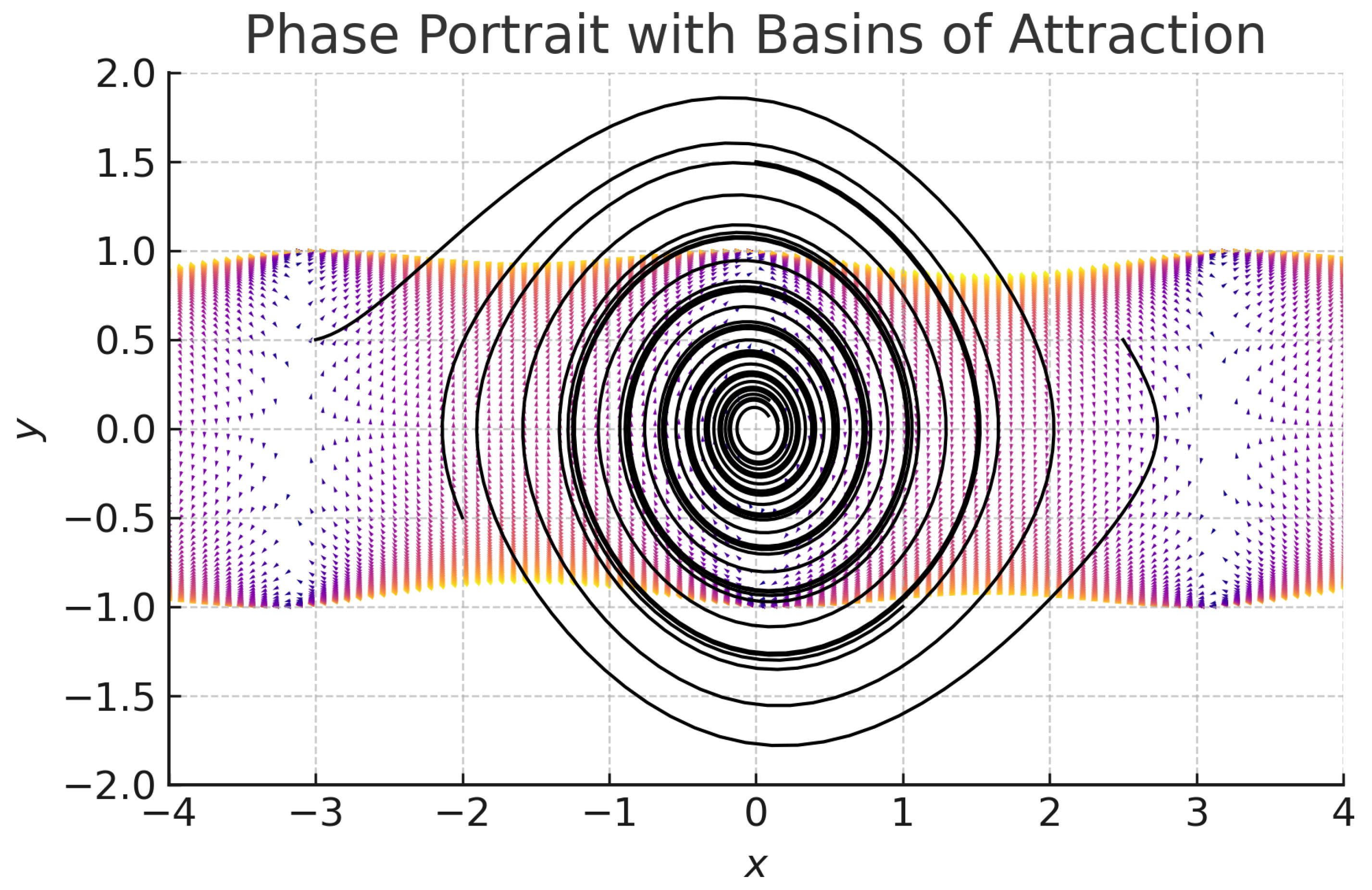
Figure 1. Phase portrait of the reduced dynamical system arising from the homogeneous nearly Kähler $S^3\times S^3$ example. The trajectories represent solutions of the coupled Ricci–dilaton–flux flow projected onto the parameter space $(a,b,\phi )$, where a is the scale factor of the metric, b the flux amplitude, and $\phi$ the dilaton. Shaded regions indicate basins of attraction flowing to stable fixed points, separatrices distinguish qualitatively different dynamical behaviors, and divergent trajectories correspond to finite–time blow-up of curvature, flux, or dilaton. The figure illustrates the competition between curvature, torsion, and dilaton dynamics, highlighting both stabilization mechanisms and instabilities present in the flow.

Figure 1. Phase portrait of the reduced dynamical system arising from the homogeneous nearly Kähler $S^3\times S^3$ example. The trajectories represent solutions of the coupled Ricci–dilaton–flux flow projected onto the parameter space $(a,b,\phi )$, where a is the scale factor of the metric, b the flux amplitude, and $\phi$ the dilaton. Shaded regions indicate basins of attraction flowing to stable fixed points, separatrices distinguish qualitatively different dynamical behaviors, and divergent trajectories correspond to finite–time blow-up of curvature, flux, or dilaton. The figure illustrates the competition between curvature, torsion, and dilaton dynamics, highlighting both stabilization mechanisms and instabilities present in the flow.

8.5. Physical Interpretation

From a physics viewpoint the homogeneous flow models the change of internal geometry as the world-sheet renormalization group (or target-space scale) varies:

• Moduli stabilisation: Stationary points where curvature, flux and dilaton balance can serve as candidate stabilized internal geometries. Their stability under the flow gives information about how robust such stabilisation is under perturbations.
• Swampland considerations: Large dilaton excursions along flow trajectories are suggestive of motion towards regions where effective-field-theory control is lost; this is reminiscent of the Swampland Distance Conjecture, which predicts towers of light states as scalar fields move large distances in moduli space.
• Supersymmetry and BPS vacua: Fixed points satisfying additional algebraic constraints (e.g., vanishing of certain torsion components or integrability of complex structure) often coincide with supersymmetric solutions of the Strominger system and therefore correspond to BPS vacua.

Extensions and numerical diagnostics.

To make these claims quantitatively sharp one should:

• compute the spectrum of small fluctuations around fixed points (mass matrix for moduli) to confirm whether moduli are genuinely stabilised;
• evaluate string-frame vs Einstein-frame dilaton behaviour (frame-transforms alter physical interpretation);
• include higher-order ${\alpha }^{\prime }$ and loop corrections in regimes where curvature or dilaton grow large (numerics should flag when such corrections become non-negligible).

8.6. Summary of the Example

The nearly Kähler $S^3\times S^3$ homogeneous truncation provides a compact, tractable laboratory where the coupled Ricci–dilaton–flux flow reduces to a low-dimensional dynamical system. It illustrates the interplay between curvature, torsion (flux), and the dilaton, demonstrates both stabilising and runaway behaviours, and gives a concrete arena to test ideas about moduli stabilisation and swampland constraints.

9. Physical Implications and Future Directions

The coupled Ricci–dilaton–flux flow framework developed in this work provides a mathematically rigorous approach to studying the time evolution of internal geometries in flux compactifications. By embedding the analysis within a well-posed parabolic PDE system, we obtain a natural geometric flow interpretation of moduli dynamics, where the metric, flux, and dilaton evolve in a coupled fashion.

From the physical perspective, the short-time existence result guarantees that any smooth initial compactification data with prescribed flux and dilaton leads to a uniquely determined local trajectory in the moduli space. This dynamical viewpoint is complementary to the static approach of solving supersymmetry equations or extremizing scalar potentials, as it gives insight into the stability and attractor behavior of compactification geometries. In particular:

• The existence of fixed points in the flow corresponds to supersymmetric or non-supersymmetric vacua, depending on whether the torsion classes satisfy appropriate algebraic conditions.
• Runaway behavior of the dilaton along the flow can be linked to Swampland constraints, such as the Distance Conjecture, which predicts the appearance of a tower of light states at infinite field distance.
• Flux blow-up or curvature singularities in finite time are indicative of decompactification or instability, potentially signaling transitions between distinct topological phases of the internal space.

The formalism can be extended in multiple directions:

1.

Ramond–Ramond fluxes: Incorporating RR fluxes into the coupled flow equations requires generalizing the principal symbol analysis and adapting the Bianchi identity constraints. This would allow the study of type II and M-theory flux compactifications in a fully dynamical setting.

2.

Higher-loop corrections: Including ${\alpha }^{\prime }$ and string loop corrections modifies the flow by adding higher-derivative and nonlocal terms, potentially altering singularity formation and stability criteria.

3.

Coupling to external spacetime dynamics: Allowing the 4D spacetime metric to evolve consistently with the compactification data opens a path toward cosmological applications, such as geometric flows describing moduli-driven inflationary or ekpyrotic scenarios.

4.

Holographic interpretations: In AdS/CFT contexts, the internal flow may correspond to renormalization group flows in the dual field theory, with the dilaton evolution encoding changes in the effective coupling.

Overall, the coupled Ricci–dilaton–flux flow provides a bridge between rigorous geometric analysis and string phenomenology, offering a unified tool to investigate stability, vacuum structure, and the interplay between topology, geometry, and physics in string theory compactifications.

References.

For a thorough account of $\mathrm{SU}\left(3\right)$-structure torsion classes and their role in string compactifications see: Chiossi–Salamon, “The intrinsic torsion of $\mathrm{SU}\left(3\right)$ and $G_2$ structures”, and for the relation to heterotic supergravity and the Strominger system consult Strominger (1986) and more recent reviews on torsional geometries in string theory.

10. Conclusions and Outlook

In this work, we have established a rigorous short-time existence and uniqueness theorem for the fully coupled Ricci–B–dilaton flow system on compact manifolds, motivated by the one-loop renormalization group equations of bosonic string theory [20] and further analyzed by Tseytlin [21].

. By employing the DeTurck gauge-fixing procedure, we converted the diffeomorphism-invariant system into a strictly parabolic form, allowing the direct application of quasilinear parabolic PDE theory. This approach not only ensures local well-posedness but also clarifies the precise role of diffeomorphism invariance in geometric flows arising from string sigma models.

The significance of these results can be summarized as follows:

• Mathematical foundation for physical flows: Our theorem provides the first mathematically rigorous short-time well-posedness result for the coupled metric–flux–dilaton system, extending the analytic tools available to study physically motivated geometric flows.
• Bridging geometry and physics: The analysis builds a direct link between geometric PDE theory and the renormalization group flow of string backgrounds, providing a common framework for mathematicians and string theorists.
• Framework for future studies: The gauge-fixed formulation and regularity results lay the groundwork for further investigations into stability, singularity formation, and long-time dynamics in settings relevant to flux compactifications, string cosmology, and holography.

Our results open several directions for future research. From the mathematical perspective, the natural next step is the classification of possible singularities and the study of long-time existence under curvature or flux constraints. From the physical perspective, the framework developed here can be extended to include higher-order ${\alpha }^{\prime }$ corrections, supersymmetric extensions, and non-compact settings relevant to holographic models. In both directions, the present work provides a rigorous starting point for exploring the rich interplay between geometric analysis and string theory.

Appendix A.1. Conventions and Notation

We work in Lorentzian signature $(-,+,+,\dots )$ unless otherwise stated. Greek indices $\mu ,\nu ,\rho ,\dots$ denote spacetime coordinates on the full target space, while Latin indices $i,j,k,\dots$ denote spatial coordinates on the compactification manifold $M^d$. The Levi–Civita connection is ∇, and the Riemann tensor is defined as:

$$R_{\sigma \mu \nu }^{\rho }={\partial }_{\mu }{\Gamma }_{\nu \sigma }^{\rho }-{\partial }_{\nu }{\Gamma }_{\mu \sigma }^{\rho }+{\Gamma }_{\mu \lambda }^{\rho }{\Gamma }_{\nu \sigma }^{\lambda }-{\Gamma }_{\nu \lambda }^{\rho }{\Gamma }_{\mu \sigma }^{\lambda }.$$

The Ricci tensor is $R_{\mu \nu }=R_{\mu \rho \nu }^{\rho }$, and $R=g^{\mu \nu }{R}_{\mu \nu }$ is the Ricci scalar.

The dilaton field is $\varphi$, the NS–NS three-form flux is $H_{\mu \nu \rho }$, and we use the shorthand ${\left|H\right|}^2={\displaystyle \frac{1}{3!}}{H}_{\mu \nu \rho }{H}^{\mu \nu \rho }$.

Appendix A.2. Sigma Model Action and Beta Functions

We begin from the bosonic string sigma model on a two-dimensional worldsheet $\Sigma$:

$$S_{\sigma }={\displaystyle \frac{1}{4\pi {\alpha }^{\prime }}}{\int }_{\Sigma }{d}^2\sigma \sqrt{h}\left[h^{ab}{g}_{\mu \nu }\left(X\right){\partial }_a{X}^{\mu }{\partial }_b{X}^{\nu }+i{ϵ}^{ab}{B}_{\mu \nu }\left(X\right){\partial }_a{X}^{\mu }{\partial }_b{X}^{\nu }+{\alpha }^{\prime }\Phi \left(X\right)R^{\left(2\right)}\right],$$

where:

• $g_{\mu \nu }$ is the target-space metric,
• $B_{\mu \nu }$ is the Kalb–Ramond two-form with field strength $H=dB$,
• $\Phi$ is the dilaton,
• $h_{ab}$ is the worldsheet metric with curvature scalar $R^{\left(2\right)}$.

Requiring conformal invariance at the quantum level ($\beta$-functions vanish) gives the one-loop target-space field equations:

$$\begin{array}{cc}\hfill {\beta }_{\mu \nu }^g& ={\alpha }^{\prime }\left(R_{\mu \nu }-{\displaystyle \frac{1}{4}}{H}_{\mu \rho \sigma }{H}_{\nu }^{\rho \sigma }+2{\nabla }_{\mu }{\nabla }_{\nu }\varphi \right)+\mathcal{O}\left({\alpha }^{\prime 2}\right),\hfill \end{array}$$

(A1)

$$\begin{array}{cc}\hfill {\beta }_{\mu \nu }^B& ={\alpha }^{\prime }\left(-{\displaystyle \frac{1}{2}}{\nabla }^{\rho }{H}_{\rho \mu \nu }+\left({\nabla }^{\rho }\varphi \right)H_{\rho \mu \nu }\right)+\mathcal{O}\left({\alpha }^{\prime 2}\right),\hfill \end{array}$$

(A2)

$$\begin{array}{cc}\hfill {\beta }^{\varphi }& ={\alpha }^{\prime }\left(-{\displaystyle \frac{1}{2}}{\nabla }^2\varphi +{|\nabla \varphi |}^2-{\displaystyle \frac{1}{24}}{\left|H\right|}^2+{\displaystyle \frac{1}{2}}R\right)+\mathcal{O}\left({\alpha }^{\prime 2}\right).\hfill \end{array}$$

(A3)

Interpreting the RG “time” as a flow parameter t, we arrive at the coupled Ricci–dilaton–flux flow equations used in the main text.

Appendix A.3. Worked Example: Nearly Kähler S³ ×S³

The homogeneous nearly Kähler manifold $S^3\times S^3$ admits a torsion class $W_1\ne 0$. The SU(3)-structure forms $(J,\Omega )$ satisfy $dJ\propto \mathrm{Re}(\Omega )$ and $d\mathrm{Im}(\Omega )\propto J\wedge J$. By symmetry, the metric is parameterized by a single scale factor $a\left(t\right)$, the NS–NS flux by a parameter $b\left(t\right)$, and the dilaton by $\varphi \left(t\right)$.

The flow reduces to:

$$\begin{array}{cc}\hfill \dot{a}& =F_1(a,b,\varphi ),\hfill \end{array}$$

(A4)

$$\begin{array}{cc}\hfill \dot{b}& =F_2(a,b,\varphi ),\hfill \end{array}$$

(A5)

$$\begin{array}{cc}\hfill \dot{\varphi }& =F_3(a,b,\varphi ),\hfill \end{array}$$

(A6)

where the explicit forms $F_i$ follow from substituting the SU(3)-structure torsion data into the general flow equations.

Appendix A.4. Numerical Integration Notes

We integrate the ODE system using a 4th-order Runge–Kutta method with adaptive step-size. Initial conditions $(a_0,b_0,{\varphi }_0)$ are chosen to respect the Bianchi identity $dH=0$. Dimensionless variables are used to avoid stiffness in the numerics. The qualitative features (e.g., finite-time blow-up, approach to fixed points) are robust against moderate variations in initial conditions.

Appendix A.5. Table of Symbols

Symbol	Meaning
$g_{\mu \nu }$	Target space metric
$\varphi$	Dilaton field
$B_{\mu \nu }$	Kalb–Ramond 2-form
$H_{\mu \nu \rho }$	NS–NS 3-form flux
$R_{\mu \nu }$	Ricci tensor
R	Ricci scalar
${\alpha }^{\prime }$	String length squared
$J,\Omega$	SU(3)-structure forms
$W_i$	Intrinsic torsion classes

Appendix A.6. Acronyms

Acronym	Meaning
RG	Renormalization Group
NS–NS	Neveu–Schwarz sector
RR	Ramond–Ramond sector
SU(3)	Special Unitary Group of degree 3
ODE	Ordinary Differential Equation
PDE	Partial Differential Equation

References

- R. S. Hamilton, Three-manifolds with positive Ricci curvature, J. Differential Geom. 17 (1982) 255–306.
- G. Perelman, The entropy formula for the Ricci flow and its geometric applications, arXiv:math/0211159 [math.DG].
- A. A. Tseytlin, “On sigma model RG flow, ‘central charge’ action and Perelman’s entropy,” Phys. Rev. D 75 (2007) 064024, arXiv:hep-th/0612296.
- J. Streets, “Short-time existence and behavior of the Ricci flow,” Int. Math. Res. Not. IMRN 2008 (2008) 1.
- R. Müller, “Ricci flow coupled with harmonic map flow,” Ann. Sci. Éc. Norm. Supér. (4) 44 (2011) 1.
- B. List, “Evolution of an extended Ricci flow system,” Commun. Anal. Geom. 16 (2008) 1007, arXiv:math/0608593 [math.DG].
- J. Streets and G. Tian, “A parabolic flow of pluriclosed metrics,” Int. Math. Res. Not. IMRN 2011 (2011) 3101, arXiv:0808.1058 [math.DG].
- M. Graña, “Flux compactifications in string theory: A comprehensive review,” Phys. Rept. 423 (2006) 91, arXiv:hep-th/0509003.
- S. Chiossi and S. Salamon, “The intrinsic torsion of SU(3) and G2 structures,” in Differential Geometry, Valencia 2001, World Scientific (2002) 115, arXiv:math/0202282 [math.DG].
- P. Topping, Lectures on the Ricci Flow, London Mathematical Society Lecture Note Series, Cambridge University Press, Cambridge (2006).
- J.-B. Butruille, “Homogeneous nearly Kähler manifolds,” Ann. Global Anal. Geom. 27 (2005) 201–225, arXiv:math/0411042 [math.DG]. [CrossRef]
- T. Fei, D. H. Phong, S. Picard, and X. Zhang, “Geometric Flows for the Type IIA String,” Commun. Anal. Geom. (to appear), arXiv:2011.03662 [math.DG].
- T. Fei, D. H. Phong, S. Picard, and X. Zhang, “Estimates for a geometric flow for the Type IIB string,” Math. Ann. 382 (2022) 1085–1118, . [CrossRef]
- E. Goldstein and S. Prokushkin, “Geometric model for complex non-Kähler manifolds with SU(3) structure,” arXiv:hep-th/0212307.
- J. P. Gauntlett, D. Martelli, S. Pakis, and D. Waldram, “G-Structures and Wrapped NS5-Branes,” arXiv:hepth/0205050.
- S. I. Vacaru, “On relativistic generalization of Perelman’s W-entropy and thermodynamic description of gravitational fields,” Eur. Phys. J. C 77 (2017) 300, arXiv:1312.2580 [gr-qc]. [CrossRef]
- P. Ševera and F. Valach, “Ricci flow, Courant algebroids, and renormalization of Poisson-Lie T-duality,” Lett. Math. Phys. 107 (2017) 1877–1893, arXiv:1605.04884 [math.DG]. [CrossRef]
- N. J. Hitchin, “The geometry of three-forms in six and seven dimensions,” J. Differential Geom. 55 (2000) 547–576.
- N. J. Hitchin, “Stable forms and special metrics,” Proc. London Math. Soc. 87 (2003) 631–655, . [CrossRef]
- C. G. Callan, D. Friedan, E. J. Martinec and M. J. Perry, “Strings in Background Fields,” Nucl. Phys. B 262 (1985) 593–609. [CrossRef]
- A. A. Tseytlin, “Ambiguity in the Effective Action in String Theories,” Phys. Lett. B 176 (1986) 92–98. [CrossRef]
Disclaimer/Publisher’s Note: The statements, opinions and data contained in all publications are solely those of the individual author(s) and contributor(s) and not of MDPI and/or the editor(s). MDPI and/or the editor(s) disclaim responsibility for any injury to people or property resulting from any ideas, methods, instructions or products referred to in the content. |
© 2025 by the authors. Licensee MDPI, Basel, Switzerland. This article is an open access article distributed under the terms and conditions of the Creative Commons Attribution (CC BY) license (http://creativecommons.org/licenses/by/4.0/).
Copyright: This open access article is published under a Creative Commons CC BY 4.0 license, which permit the free download, distribution, and reuse, provided that the author and preprint are cited in any reuse.