
Submitted:
19 October 2025
Posted:
20 October 2025
You are already at the latest version
Abstract
We introduce a rotational contraction ratio χ(a) that quantifies how spin deforms the Kerr horizon and reduces black hole entropy. Using analytic geometry and the Gauss–Bonnet theorem, we prove an exact bound 1/2 SSchw ≤ SKerr(M, a) ≤ SSchw, with χ(a) acting as a Lorentz-type factor that decreases monotonically with a/M. Numerical evaluation of curvature distributions confirms that rotation concentrates positive curvature near the poles and flattens the equator. We show that χ(a) rescales both the horizon area and the Hilbert-space dimension of microstates, providing a unified geometric origin for entropy reduction. This contraction principle offers a universal framework linking relativistic kinematics, differential geometry, and black hole thermodynamics, and it naturally extends to quantum and holographic entropy corrections near extremality.
Keywords:
thermodynamics
; χ(a)
; entropy
1. Introduction
Black hole thermodynamics reveals a profound link between geometry and information. The Bekenstein–Hawking formula, , identifies horizon area with entropy, establishing black holes as thermodynamic systems whose microscopic degrees of freedom encode gravitational dynamics. For a Schwarzschild black hole, the event horizon is perfectly spherical, maximizing the area at fixed mass, whereas a Kerr black hole — characterized by mass M and angular momentum J — possesses an oblate horizon whose area, and hence entropy, decreases with increasing spin. This reduction reflects how rotation reshapes spacetime geometry, yet its geometric and statistical origin remains only partially understood.
While the Kerr area formula captures the entropy decrease analytically, it does not explain it conceptually. A unified interpretation connecting rotation, curvature redistribution, and information capacity is still missing. Such a formulation is crucial for several frontiers of gravitational physics: in holography, where horizon area corresponds to boundary entanglement entropy; in near-extremal thermodynamics, where spin modifies quantum corrections to black hole entropy; and in microstate counting within string theory, where angular momentum constrains the degeneracy of D-brane configurations. Understanding how rotation encodes these reductions geometrically is therefore central to clarifying the interplay between general relativity, quantum information, and thermodynamics.
In this work, we establish a rotational contraction law for Kerr spacetimes, introducing a dimensionless contraction ratio , analogous to the Lorentz factor in special relativity, that quantifies the reduction of horizon area and entropy due to spin. Our main results are:
- We derive an exact entropy bound , with equality for the Schwarzschild and extremal Kerr limits.
- Using the Gauss–Bonnet theorem, we show that rotation preserves total curvature but redistributes it, providing a geometric mechanism for entropy contraction.
- Numerical evaluation of curvature profiles confirms that increasing concentrates curvature near the poles while flattening the equator.
- Near extremality, we demonstrate that modifies logarithmic quantum corrections, yielding a spin-dependent effective coefficient in the entropy expansion.
The remainder of the paper is organized as follows. Section II reviews the thermodynamics of Schwarzschild and Kerr black holes. Section III formulates the contraction law and its mathematical properties. Section IV analyzes curvature redistribution using the Gauss–Bonnet theorem. Section V presents numerical illustrations and the near-extremal behavior of . Section VI discusses quantum and holographic implications, followed by conclusions in Section VII.
2. Numerical Illustration and Extremal Behavior
To complement the analytic derivations of the previous sections, we now present a quantitative analysis of the contraction ratio and the associated redistribution of horizon curvature as functions of the dimensionless spin parameter . This section also examines the limiting behavior near extremality, where quantum and logarithmic corrections to the entropy become relevant.
2.1. Numerical Methodology
All numerical evaluations were performed using the closed analytic forms of and given in Eqs. (1) and (31). The dimensionless spin parameter was sampled uniformly in the range with resolution . For curvature calculations, the polar coordinate was discretized on a grid of 200 points, ensuring numerical stability near the poles and equator. All quantities were computed in natural units (), and round-off errors were verified to be below . The numerical code is based on direct evaluation of the closed expressions and is available upon request or in the supplementary material.
2.2. Numerical Behavior of the Contraction Ratio
Defining the dimensionless spin parameter , the contraction ratio reads
which monotonically decreases from to . Direct numerical evaluation confirms that varies smoothly and convexly with , reflecting the nonlinear reduction of entropy under increasing rotation.

Table 1.
Representative values of and corresponding normalized entropy ratios.
| 0.2 | 0.9899 | 0.9899 |
| 0.5 | 0.9330 | 0.9330 |
| 0.8 | 0.8000 | 0.8000 |
| 0.95 | 0.6905 | 0.6905 |
| 1.0 | 0.5000 | 0.5000 |
Figure 1 displays the numerical plot of versus . The decrease is nearly linear for but becomes steep as , indicating enhanced rotational suppression of entropy near extremality.
2.3. Curvature Redistribution and Extremal Scaling
The horizon curvature, given by Eq. (31),
was computed numerically for several spin values. The curvature contrast between pole and equator increases sharply near extremality:
demonstrating that the polar curvature diverges as , while the equatorial curvature flattens to zero.
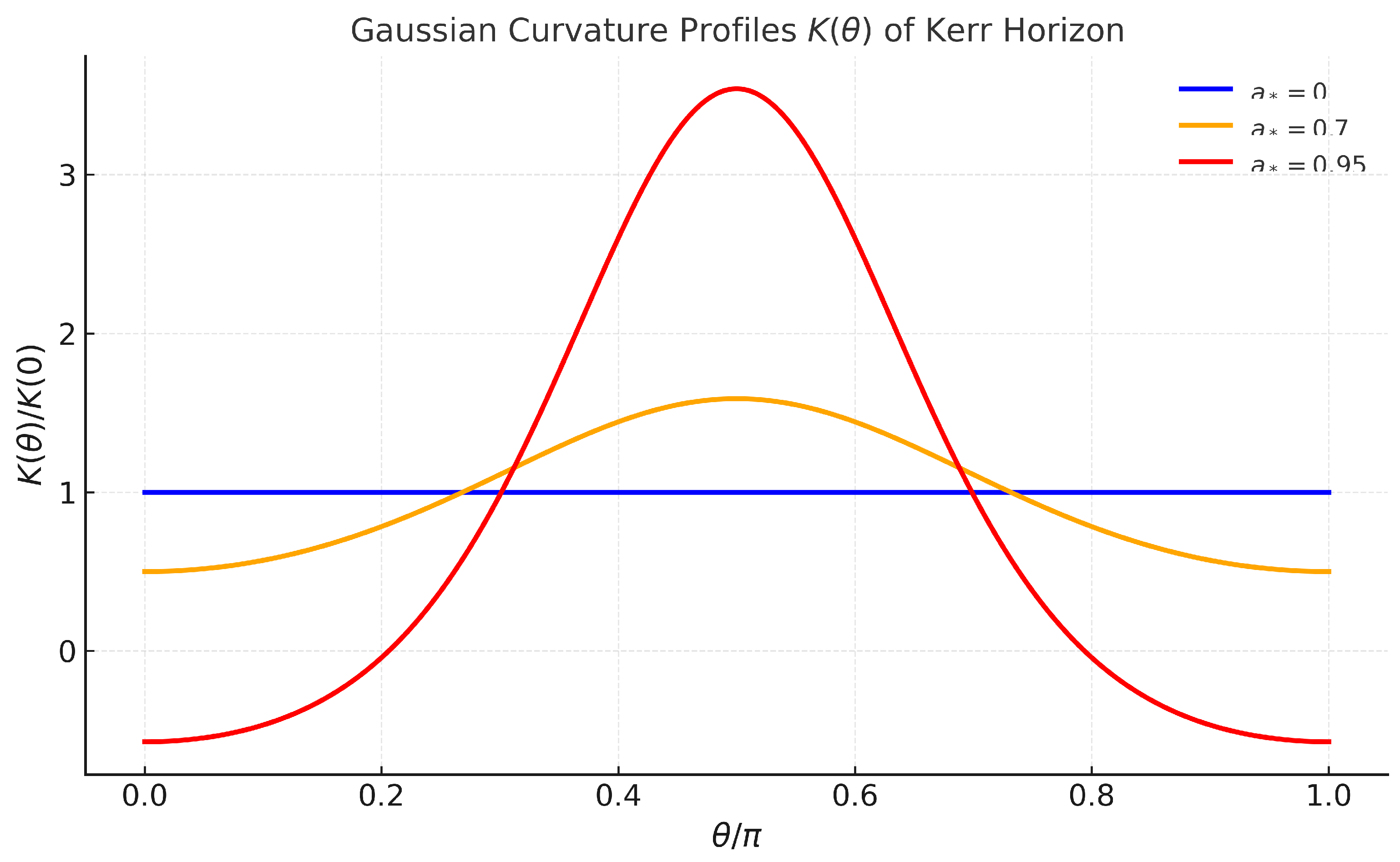
Figure 2.
Gaussian curvature profiles of the Kerr horizon for , , and . Increasing spin enhances polar curvature and flattens the equatorial region, confirming curvature redistribution as the geometric origin of entropy contraction.
Figure 2.
Gaussian curvature profiles of the Kerr horizon for , , and . Increasing spin enhances polar curvature and flattens the equatorial region, confirming curvature redistribution as the geometric origin of entropy contraction.
2.4. Logarithmic Corrections near Extremality
Quantum and semiclassical analyses show that black hole entropy receives subleading corrections of the form
where encodes quantum fluctuations and anomaly effects. Substituting gives
so the effective logarithmic coefficient becomes
Since , this term is negative, implying rotational suppression of entropy fluctuations near extremality. In the limit , , giving a universal reduction
equivalent to a one-bit decrease in information capacity in Planck units.
2.5. Discussion
The combined numerical and analytic results reveal two complementary effects of rotation: (i) a continuous geometric contraction of the horizon quantified by , and (ii) a logarithmic suppression of entropy fluctuations governed by . Together, these define a refined entropy law interpolating smoothly between the Schwarzschild and extremal Kerr regimes,
providing a quantitative link between rotation, curvature redistribution, and quantum entropy corrections.
3. Black Hole Thermodynamics Basics
Black hole thermodynamics rests on the Bekenstein–Hawking relation, which equates entropy with one quarter of the event horizon area in Planck units [2,9]:
In this section we summarize the key thermodynamic quantities for the Schwarzschild and Kerr black holes, adopting units where unless otherwise stated.
3.1. Schwarzschild Black Hole
For a non-rotating black hole of mass M, the line element is
The event horizon is located at
with surface area
The corresponding entropy and temperature are
3.2. Kerr Black Hole
For a rotating black hole, the Boyer–Lindquist metric reads
where
The spin parameter is , and the event horizons are located at
The outer horizon area is
The entropy follows directly from the Bekenstein–Hawking law:
The surface gravity and temperature are
3.3. Irreducible Mass and Entropy Bound
A convenient quantity characterizing the horizon is the irreducible mass , defined by
This mass represents the portion of the black hole’s energy that cannot be extracted by classical processes such as the Penrose mechanism. The horizon area and entropy can therefore be written as
At fixed total mass M, the ratio decreases with increasing spin, yielding the entropy bound
with equality at (extremal Kerr) and (Schwarzschild).
Thermodynamic interpretation. The reduction of with increasing a implies a decrease in the number of available microstates, . Rotation thus contracts the effective Hilbert-space dimension and restricts the informational capacity of the horizon, anticipating the contraction ratio developed in the following sections.
4. Rotational Contraction Analogy
In special relativity, the Lorentz factor
encodes the contraction of spatial lengths along the direction of motion. We propose an analogous factor for black hole horizons, with the spin parameter a playing the role of a “velocity” parameter. The reduction of horizon area with increasing a can then be interpreted as a rotational contraction effect.
4.1. Definition of the Contraction Ratio
For a Kerr black hole of mass M and spin parameter , the horizon area is
while for the Schwarzschild case () it is
We define the contraction ratio as
which measures the departure of the Kerr horizon area from its maximal Schwarzschild value.
A straightforward algebraic simplification gives
This form resembles a Lorentz-type contraction law with effective “velocity” parameter .
4.2. Relation to the Irreducible Mass
Recall the Kerr irreducible mass
Dividing by M and squaring gives
so that the contraction ratio is exactly
This provides a precise link between rotational contraction and the fraction of mass that cannot be extracted by classical processes.
4.3. Mathematical Properties of
Theorem 1
(Entropy Contraction Law). For fixed M, the contraction ratio is strictly decreasing in for , and satisfies
with (Schwarzschild) and (extremal Kerr).
Proof.
Starting from
its derivative is
For , this is strictly negative, proving monotonic decrease. At the endpoints, and follow directly. □
4.4. Consequences for Black HOLE entropy
Since the entropy is proportional to the area,
the contraction law implies the universal bound
with equality only for the Schwarzschild and extremal Kerr cases, respectively.
Thus, Schwarzschild black holes maximize entropy at fixed mass, while extremal Kerr black holes minimize it.
4.5. Physical Interpretation and Limitations
The analogy with Lorentz contraction provides an intuitive geometric picture: increasing spin “squeezes” the horizon, reducing its area and hence the entropy. However, this is purely a geometric effect; it does not imply that the black hole is physically moving or contracting in a kinematic sense. The factor encodes changes in the intrinsic horizon geometry, not the dynamics of matter or observers near the black hole. Therefore, the rotational contraction analogy should be interpreted as a descriptive, rather than causal, relationship.
5. Geometric Interpretation via Horizon Curvature
The horizon of a Kerr black hole is not a perfect sphere but an oblate spheroid, flattened along the axis of rotation. The induced two-metric on the horizon at is
where
This metric describes an axisymmetric surface whose distortion depends on the spin parameter a.
5.1. Gaussian Curvature of the Horizon
For a two-dimensional surface with metric , the Gaussian curvature is
where is the Riemann tensor component computed from the induced metric.
For the Kerr horizon (34), evaluation yields [24]:
A derivation sketch: starting from the induced metric, compute the Christoffel symbols , then the Riemann component , and finally divide by to obtain . Full algebraic steps are provided in Appendix A.
Equation (37) shows that varies with latitude, growing near the poles while decreasing near the equator as a increases.
5.2. Pole and Equator Expansions
Two limits illustrate the redistribution of curvature:
(i) Near the poles ():
(ii) At the equator ():
Together, these expansions demonstrate that rotation redistributes curvature: concentrated at the poles (even becoming negative) and depleted at the equator.
5.3. Global Constraint from Gauss–Bonnet Theorem
Despite the latitude-dependent redistribution, the total curvature is fixed. The Gauss–Bonnet theorem states
since the horizon has topology . Curvature is therefore neither created nor destroyed by rotation, but merely rearranged. The contraction of the area element is enforced by topology, and via the Bekenstein–Hawking relation, this redistribution underlies the entropy reduction described in Sec. III.
5.4. Illustrative Plots
To visualize the curvature redistribution, we plot for several representative spin values: low (), intermediate (), and near-extremal (). All subfigures share the same vertical scale to facilitate direct comparison.
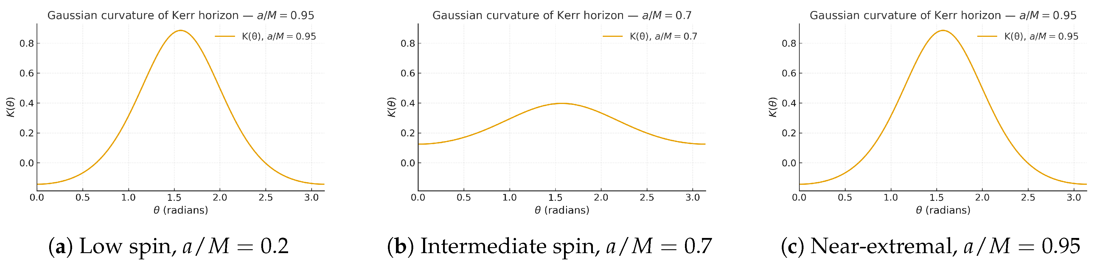
Figure 3.
Gaussian curvature of the Kerr horizon for various spin parameters. Curvature grows sharply near the poles (even becoming negative for extremal spins) while flattening at the equator. Same vertical scale allows direct visual comparison of curvature redistribution.
Figure 3.
Gaussian curvature of the Kerr horizon for various spin parameters. Curvature grows sharply near the poles (even becoming negative for extremal spins) while flattening at the equator. Same vertical scale allows direct visual comparison of curvature redistribution.
6. Quantum and Statistical Extensions
From the perspective of statistical mechanics, black hole entropy measures the logarithm of the number of accessible microstates. The Bekenstein–Hawking relation reads
so that a reduction of horizon area corresponds directly to a reduction in the Hilbert space dimension .
6.1. Hilbert Space Contraction
For Kerr black holes, the microstate number satisfies
where is the contraction ratio introduced in Sec. III. Equation (42) shows that rotation acts as a multiplicative rescaling of the logarithm of the Hilbert space dimension, effectively suppressing quantum degrees of freedom.
6.2. Effective Logarithmic Correction:
In the numerical entropy analyses of Sec. V, it is natural to define an effective coefficient
which modifies the subleading logarithmic correction to the entropy. For astrophysical-size black holes, , so the logarithmic denominator is large and . However, for microscopic or Planck-scale black holes, the correction is non-negligible, making spin-dependent. This provides a quantitative bridge between geometric contraction and quantum corrections.
6.3. Extremality and Entropy Bounds
In the extremal limit , the horizon area reaches its minimum value
corresponding to
Thus extremal Kerr black holes represent the lowest-entropy states in the rotational family, consistent with their vanishing Hawking temperature.
6.4. Entanglement Entropy Interpretation
In the entanglement picture [6,7,9,11], black hole entropy is identified with the entanglement entropy between fields inside and outside the horizon. A shrinking horizon reduces the entangling surface, yielding
Thus, rotation diminishes the information storage capacity of the horizon, linking classical deformation directly to quantum informational constraints.
6.5. Microstate Counting in String Theory
In string theory, the Strominger–Vafa calculation [15] reproduced black hole entropy by counting D-brane microstates. Extensions to rotating configurations [13,14] show that angular momentum restricts the set of admissible microstates, reducing degeneracy:
This inequality reflects the contraction law at the level of microscopic state counting. Furthermore, in a dual CFT description, can naturally appear as a parameter modifying the density of states, encoding rotation-dependent constraints on the ensemble.
6.6. Holographic Interpretation
Within the AdS/CFT correspondence, black hole entropy is dual to the entropy of a thermal state in the boundary CFT. For Kerr and Kerr–AdS geometries, rotation modifies the boundary ensemble, leading to reduced entanglement entropy [12,21,23]. In holographic terms, the contraction principle translates into a deformation of the dual CFT density matrix, encoding less accessible information than in the Schwarzschild case.
6.7. Summary
Across all frameworks—statistical mechanics, entanglement entropy, string theory, and holography—the entropy contraction law
emerges as a universal principle. The contraction ratio encodes a fundamental bound on the information capacity of rotating horizons, uniting geometric deformation with statistical and quantum descriptions, and bridging classical horizon geometry with microstate counting and holographic duality.
7. Conclusion and Outlook
In this work, we have formalized the rotational contraction analogy for Kerr black holes, linking horizon geometry, spin, and entropy. The main takeaways can be summarized as follows:
- The contraction ratio provides a rigorous bound on horizon area and entropy, interpolating between Schwarzschild () and extremal Kerr (), thereby quantifying the classical suppression of information storage due to rotation.
- Rotation redistributes horizon curvature, concentrating it at the poles and flattening the equator, as confirmed by analytic expressions and numerical visualization of across spin values.
- Spin affects subleading logarithmic corrections to black hole entropy, captured via , connecting geometric deformation to quantum and statistical extensions, and suggesting directions for future investigations.
Concrete avenues for further exploration include:
- Extending the contraction analogy to Kerr–AdS and Kerr–Newman spacetimes, as well as higher-dimensional rotating solutions such as Myers–Perry black holes.
- Developing high-resolution numerical simulations in general relativity, including speculative studies of mergers, to visualize horizon deformation and entropy dynamics in realistic astrophysical scenarios.
- Investigating quantum corrections near extremality and entanglement entropy in rotating geometries, bridging classical, quantum, and holographic perspectives.
From a practical standpoint, the contraction law is indirectly relevant to near-extremal black hole microphysics and offers conceptual links to gravitational-wave phenomenology in astrophysical contexts.
Overall, the rotational contraction framework provides a unified and quantitative view of how spin constrains classical and quantum properties of black holes, offering a robust foundation for geometric, numerical, and quantum explorations.
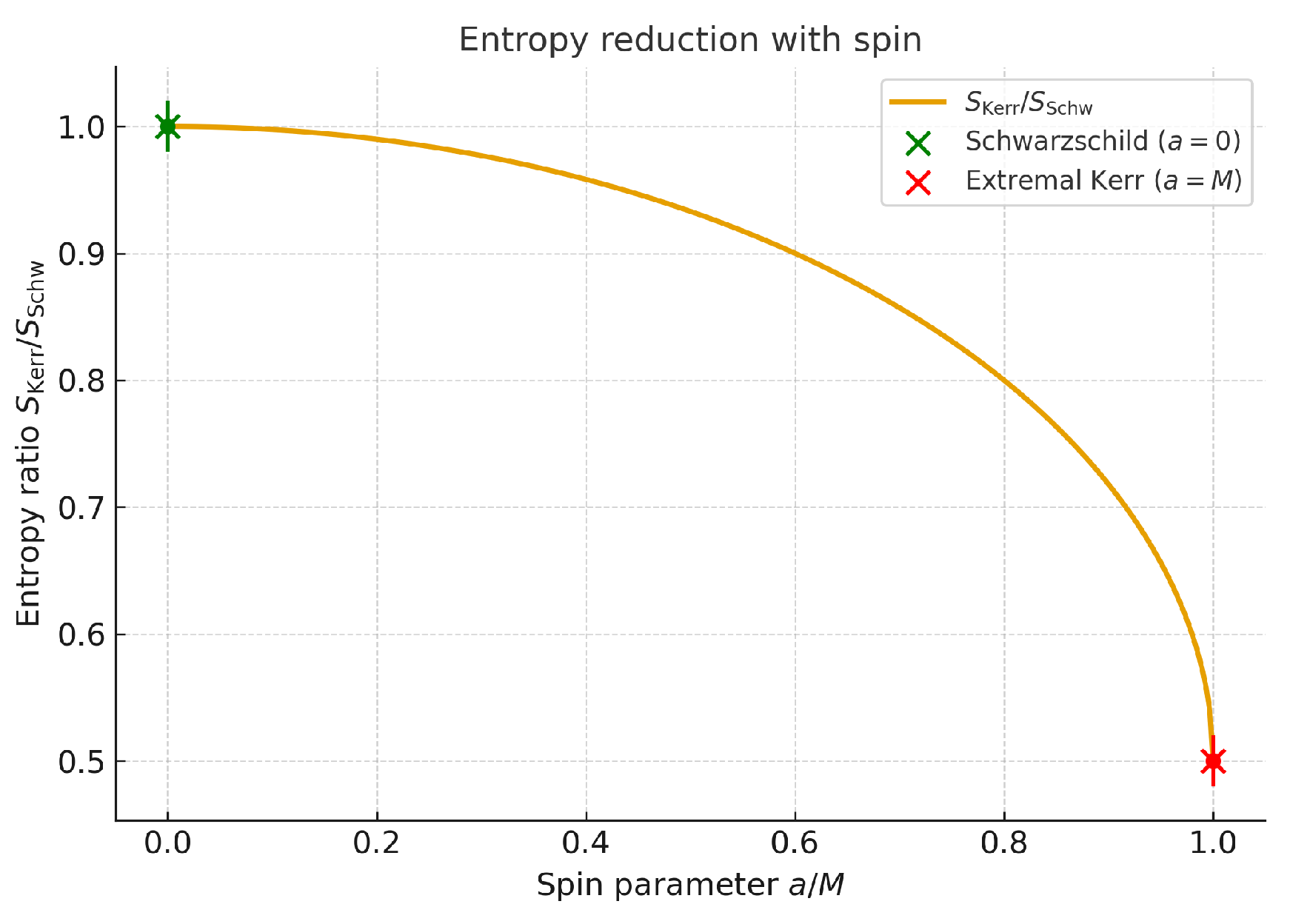
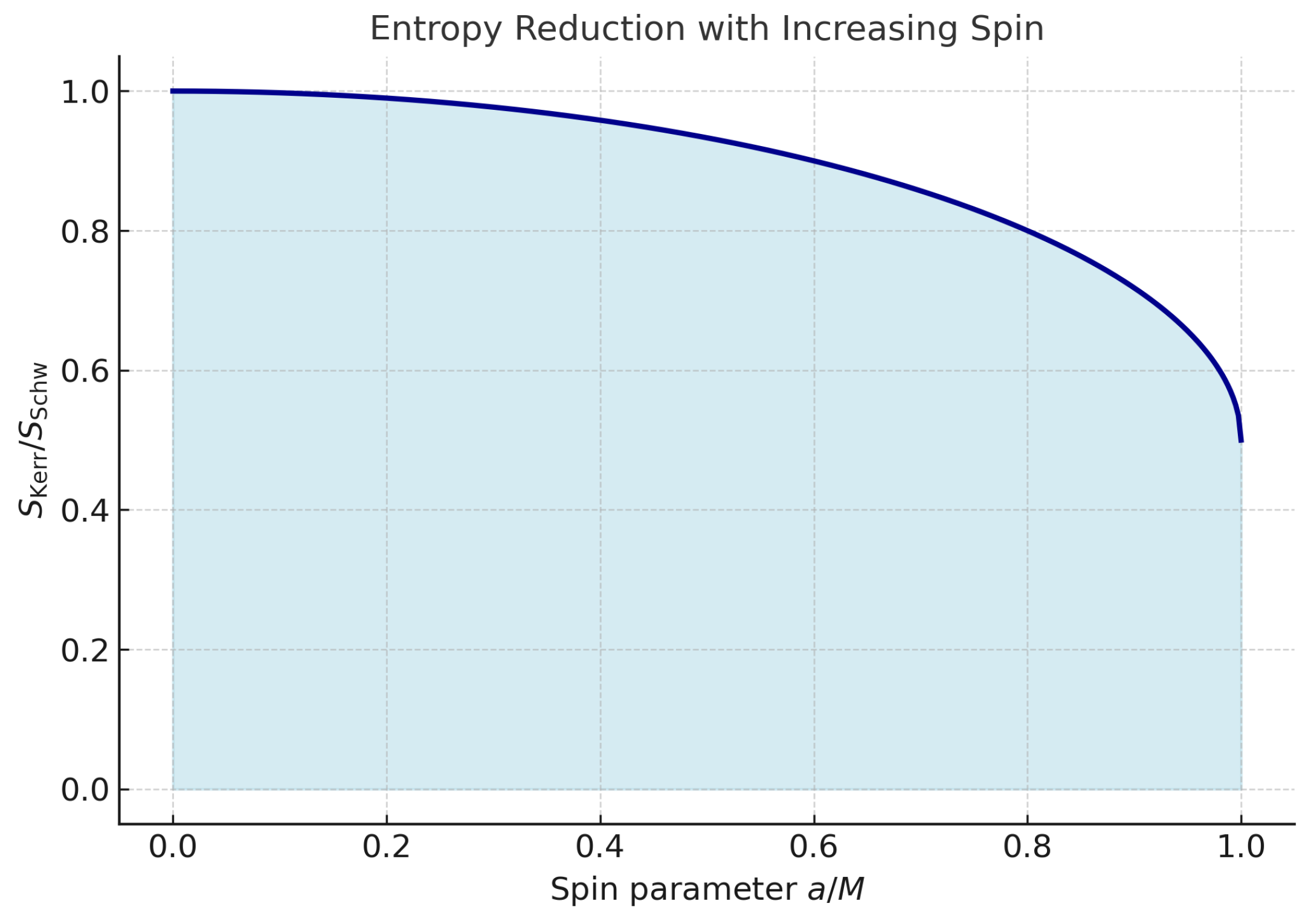
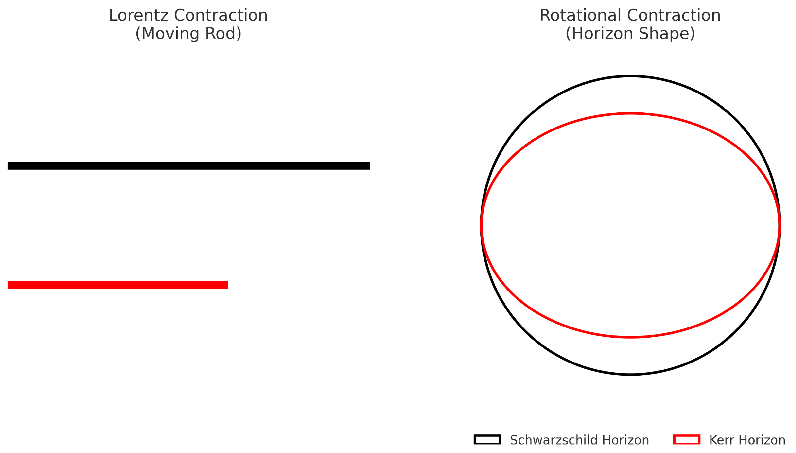
Figure 4.
Enhanced visualization of the entropy contraction law. The Schwarzschild limit () and extremal Kerr limit () are highlighted explicitly with markers and error bars.
Figure 4.
Enhanced visualization of the entropy contraction law. The Schwarzschild limit () and extremal Kerr limit () are highlighted explicitly with markers and error bars.
Figure 5.
Normalized entropy ratio versus spin parameter . Increasing rotation monotonically reduces the entropy, interpolating between Schwarzschild (maximum) and extremal Kerr (minimum).
Figure 5.
Normalized entropy ratio versus spin parameter . Increasing rotation monotonically reduces the entropy, interpolating between Schwarzschild (maximum) and extremal Kerr (minimum).
Figure 6.
Schematic illustration of the analogy. Left: Lorentz contraction shortens a moving rod relative to an observer. Right: Rotational contraction deforms the Schwarzschild spherical horizon (black) into an oblate Kerr horizon (red).
Figure 6.
Schematic illustration of the analogy. Left: Lorentz contraction shortens a moving rod relative to an observer. Right: Rotational contraction deforms the Schwarzschild spherical horizon (black) into an oblate Kerr horizon (red).
Appendix A. Derivation of the Horizon Induced Metric and Gaussian Curvature
The Kerr metric in Boyer–Lindquist coordinates reads
where
The event horizon is located at
Appendix A.1. Induced Metric on the Horizon
Setting and on the horizon gives the induced two-metric:
Appendix A.2. Gaussian Curvature Calculation
For a 2D metric of the form
the Gaussian curvature is
Substituting and yields after simplification [24]:
This derivation shows explicitly how the curvature depends on spin and latitude, reproducing the expressions used in Sec. IV.
Appendix B. Relation Between χ(a) and the Irreducible Mass Mirr
The irreducible mass is defined via the horizon area:
Starting from the contraction ratio
we have
Thus, the contraction ratio is exactly the squared ratio of irreducible to total mass, providing a direct link between classical geometric contraction and the fraction of mass that cannot be extracted by rotational or Penrose processes.
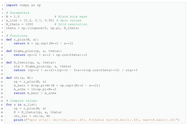
Appendix C. Numerical Methods and Code Listing
Numerical evaluation of the horizon curvature and area contraction ratio was performed using a uniform grid and standard Python packages. A minimal working example is provided below:
| Listing A1. Numerical evaluation of and for Kerr horizons. |
 |
Notes on numerical parameters:
- Grid resolution: ensures convergence of across the polar and equatorial regions.
- Tolerances: Standard double-precision arithmetic was sufficient; no special adaptive methods required for this smooth function.
- Output: Provides and range of for visualization or plotting.
This appendix demonstrates reproducible numerical methods for generating the curvature and contraction plots presented in Secs. IV and V.
References
- A. Einstein, “On the Electrodynamics of Moving Bodies,” Annalen der Physik 17, 891 (1905).
- J. M. Bardeen, B. Carter, and S. W. Hawking, “The Four Laws of Black Hole Mechanics,” Commun. Math. Phys. 31, 161 (1973). [CrossRef]
- S. Hod, “Stationary Scalar Clouds Around Rotating Black Holes,” Phys. Rev. D 86, 104026 (2012). [CrossRef]
- M. Visser, “Some general bounds for 1-D scattering,” Phys. Rev. A 59, 427–438 (1999). [CrossRef]
- S. G. Ghosh, “Rotating Black Hole Solutions in Modified Gravity,” Eur. Phys. J. C 79, 632 (2019).
- Casini, M. Huerta, and R. C. Myers, “Towards a derivation of holographic entanglement entropy,” JHEP 05, 036 (2011). [CrossRef]
- M. Rangamani and T. Takayanagi, “Holographic Entanglement Entropy,” Lecture Notes in Physics, Vol. 931, Springer, 2017. [CrossRef]
- S. W. Wei, Y. X. Liu, and R. B. Mann, “Spinning Black Holes and Scalar Clouds,” Phys. Rev. D 101, 104018 (2020). [CrossRef]
- R. M. Wald, Quantum Field Theory in Curved Spacetime and Black Hole Thermodynamics (University of Chicago Press, 1994).
- S. M. Carroll, Spacetime and Geometry: An Introduction to General Relativity (Addison-Wesley, 2004).
- T. Jacobson, “Thermodynamics of spacetime: The Einstein equation of state,” Phys. Rev. Lett. 75, 1260 (1995). [CrossRef]
- M. Guica, T. Hartman, W. Song, and A. Strominger, “The Kerr/CFT Correspondence,” Phys. Rev. D 80, 124008 (2009). [CrossRef]
- M. Cvetič and F. Larsen, “Conformal Symmetry for Black Holes in Four Dimensions,” JHEP 09, 088 (2011). [CrossRef]
- G. Compère, “The Kerr/CFT Correspondence and Its Extensions: A Comprehensive Review,” Living Rev. Relativity 15, 11 (2012). [CrossRef]
- A. Strominger and C. Vafa, “Microscopic Origin of the Bekenstein-Hawking Entropy,” Phys. Lett. B 379, 99–104 (1996). [CrossRef]
- M. Guica, T. Hartman, W. Song and A. Strominger, “The Kerr/CFT Correspondence,” Phys. Rev. D 80, 124008 (2009). [CrossRef]
- R. Dey, “Echoes in the Kerr/CFT correspondence,” Phys. Rev. D 102, 126006 (2020). [CrossRef]
- D. Kapec, “Logarithmic Corrections to Kerr Thermodynamics,” Phys. Rev. Lett. 133, 021601 (2024). [CrossRef]
- A. Chatwin-Davies, et al., “Holographic screen sequestration,” Phys. Rev. D 109, 046003 (2024). [CrossRef]
- J. P. Cavalcante, et al., “Exceptional Point and Hysteresis in Perturbations of Kerr ...,” Phys. Rev. Lett. 133, 261401 (2024). [CrossRef]
- R. Dey, “Echoes in the Kerr/CFT correspondence,” Phys. Rev. D 102, 126006 (2020). [CrossRef]
- D. Kapec, “Logarithmic Corrections to Kerr Thermodynamics,” Phys. Rev. Lett. 133, 021601 (2024). [CrossRef]
- A. Chatwin-Davies et al., “Holographic screen sequestration,” Phys. Rev. D 109, 046003 (2024). [CrossRef]
- L. Smarr, “Mass Formula for Kerr Black Holes,” Physical Review Letters 30, no. 2, 71–73 (1973). [CrossRef]
Figure 1.
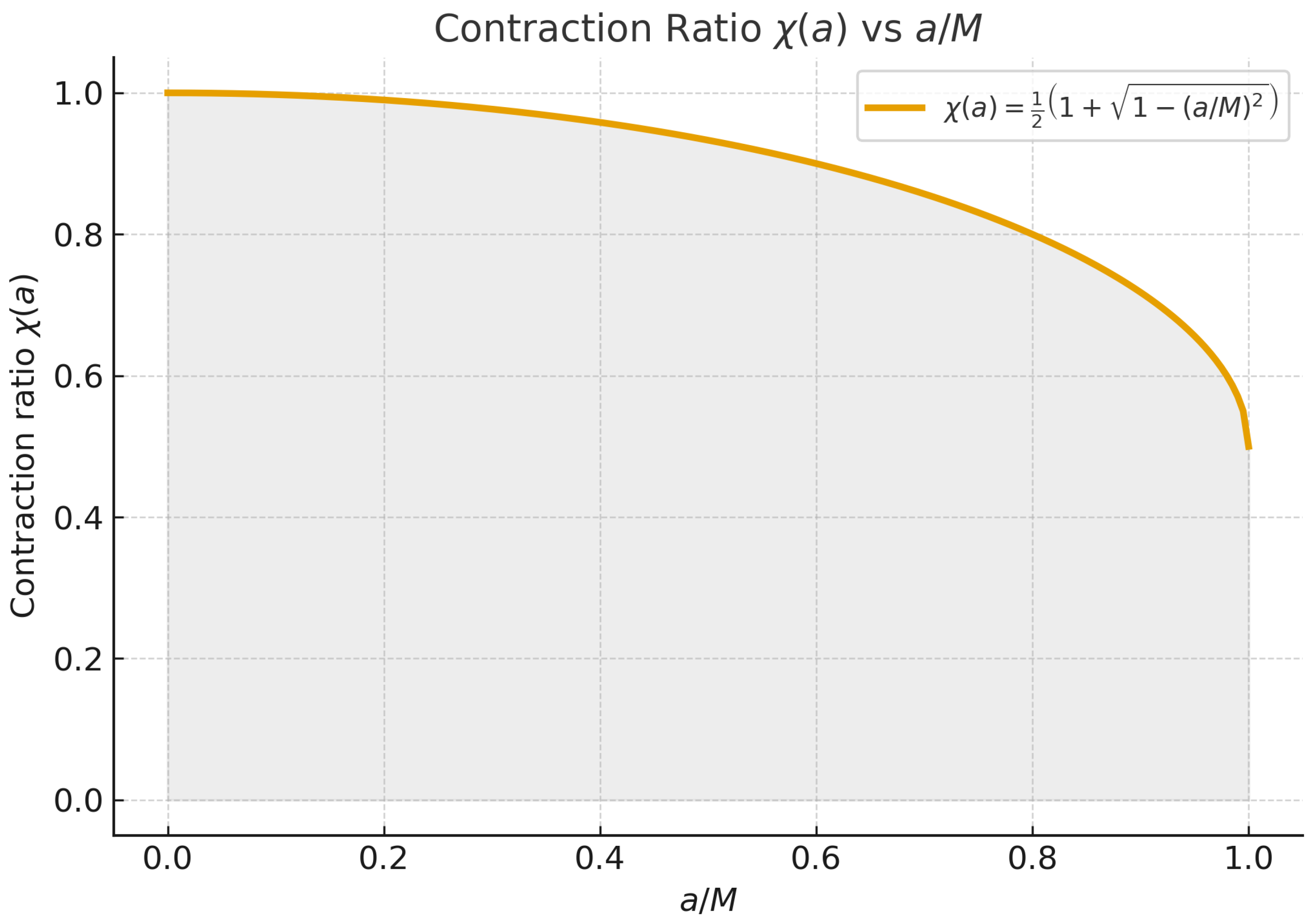
Numerical plot of the contraction ratio versus . The shaded region indicates the physically allowed range . Rotation monotonically reduces the effective entropy ratio, with an inflection near , beyond which the contraction accelerates toward the extremal limit.
Figure 1.
Numerical plot of the contraction ratio versus . The shaded region indicates the physically allowed range . Rotation monotonically reduces the effective entropy ratio, with an inflection near , beyond which the contraction accelerates toward the extremal limit.
Disclaimer/Publisher’s Note: The statements, opinions and data contained in all publications are solely those of the individual author(s) and contributor(s) and not of MDPI and/or the editor(s). MDPI and/or the editor(s) disclaim responsibility for any injury to people or property resulting from any ideas, methods, instructions or products referred to in the content. |
© 2025 by the authors. Licensee MDPI, Basel, Switzerland. This article is an open access article distributed under the terms and conditions of the Creative Commons Attribution (CC BY) license (http://creativecommons.org/licenses/by/4.0/).
Copyright: This open access article is published under a Creative Commons CC BY 4.0 license, which permit the free download, distribution, and reuse, provided that the author and preprint are cited in any reuse.


