
Submitted:
13 August 2025
Posted:
15 August 2025
You are already at the latest version
Abstract
With the increasing saturation of renewable energy sources (RES), there are growing limitations on the ability to connect new sources due to the lack of suitable locations or grid constraints. The existing renewable sources connected to the grid, in turn, pose problems related to generation variability, requiring the maintaining of costly reserves, and overproduction, resulting in forced outages. Therefore, grid operators were forced to adopt a more flexible approach when issuing connection permits, the so-called "cable pooling", which limits only the power fed into the network in a given node, not the total power of the connected sources. The article shows a method for optimal (from the investor's point of view) sizing of combination of different RES sources connected to the high-voltage network under cable pooling conditions. The most frequently used RES technologies: photovoltaics and wind turbines supplemented by the lithium-ion battery energy storage system are used. The main aim of the work is to examine the relationship between the optimally selected composition of devices and variables such as the investor's financial goal, the type of market from which they will derive revenues and prices on that market with an emphasis on the profitability of energy storage system.
Keywords:
optimal sizing
; hybrid renewable energy sources
; cable pooling
; energy storage systems
1. Introduction
With the increasing saturation of renewable energy sources (RES), there are growing limitations on the ability to connect new sources due to the lack of suitable locations or grid constraints [1]. The existing renewable sources connected to the grid, in turn, pose problems related to generation variability, requiring the maintaining of costly reserves, and overproduction, resulting in forced outages. Therefore, grid operators who previously assumed the sum of the power of various sources and storage devices connected at one connection point in the grid connection conditions are forced to adopt a more flexible approach, the so-called “cable pooling”, which limits only the power fed into the network in a given node and not the total power of the connected sources. This allows for a more economical and flexible solution consisting of connecting several different RES technologies and energy storage systems (ESS) to one network node, together forming a hybrid renewable energy source (HRES). This makes it possible to locate RES of higher capacity in a given location while creating a more stable power source. This issue has been already reflected in the regulations. In Poland, the existing regulation [2] enables the connection of two or more renewable energy source installations, which may belong to one or more producers, to the common connection point and the submitted amendment [3] proposes the inclusion of ESS in the cable pooling formula. Hungary has introduced mandatory ESS co-location for solar photovoltaic (PV) assets above a certain size. In France co-located ESS and PV can participate in the Contract for Differences (auctions with high strike prices) [4]. The issue of connecting various renewable energy sources limited by the connection power or considering the connection cost is the subject of a few articles. Among others, the work [5] discusses the issue of connecting a hydroelectric power plant with floating PV (FPV) located in the reservoir next to the power plant, the work [6] – connecting FPV with an offshore wind farm and wave energy converters. S. Golroodbari et al. in the article [7] try to assess the feasibility of adding an offshore FPV farm to an existing Dutch offshore wind farm in the North Sea, under the constraint of a certain fixed cable capacity. The specific capacity of the cable that connects the offshore park to the onshore grid is not fully used due to the limited capacity factor of the wind farm.
The issue of FPV is also related to the work [8], which concludes with the possibility of integrating different renewable technologies with the existing FPVs and highlights the benefits of doing so with some examples. The possibilities of increasing the PV potential by locating new sources at the connection points of the existing hydroelectric plants are shown in the article [9]. The RES installed power and energy increase by combining PV and wind turbine (WT) sources is shown in articles [10] and [11]. K. Obradović et al. [12] analyze how the physical design of PV/WT HRES differs from single-technology facilities, with a particular focus on spatial layout optimization, electrical design, and macro siting. Problems related to the location of WT and PV farms in the same area and the shading of panels by turbine structures and rotor blades, are discussed in [13]. An example of a spatio-temporal decision-making model which evaluates utility-scale PV, onshore WT, and hybrid PV/WT power development while techno-economic potential considers technology-specific parameters and infrastructure costs is presented in [14].
The task of optimizing the composition of HRES also appears in several publications. Most of them concern isolated HRES, often based on solutions for real locations without grid connection. In publication [15] the Mixed Integer Linear Programming (MILP) optimization algorithm has been developed to design an optimal hybrid system composed by solar, wind and diesel generators together with a battery storage for a mountain hut located in South Tyrol (Italy). The particle swarm optimization for optimal sizing of a solar-wind-battery HRES for a rural community in Rivers State, Nigeria was designed in [16]. The objective is to minimize the total economic cost, the total annual system cost and the levelized cost of energy. A two-step approach was used. The Hybrid Optimization Model for Multiple Energy Resources (HOMER) Pro Software was used in [17] to minimize the net present cost, cost of energy, and CO2 emissions of the hybridized energy system (i.e., solar, wind, and diesel) with battery storage in Bangladesh’s northern area. Medina-Santana et al. in [18] proposed a sizing methodology that includes long short-term memory cells to predict weather conditions in the long term, multivariate clustering to generate different weather scenarios, and a nonlinear mathematical formulation to find the optimal sizing of an HRES for a rural community in the Pacific Coast of Mexico. K. Kusakana et al. in [19] proposed linear programming to optimize the initial cost of the system’s components in PV/WT islanded HRESs. The task to optimize the sizing of the system components for smooth system operation and cost-effectiveness was solved in [20], with a new hybrid optimizer setup called the Jaya-Grey Wolf Optimizer. The combined objectives of minimizing net annual cost and loss of supply power probability were achieved for a standalone microgrid environment. Genetic Algorithm and Particle Swarm Optimization tools were applied in [21] to select the optimum size of RES consisting of PV modules, WT, and battery ESS (BESS).
The issue of the optimal selection of HRES structure to ensure the coverage of the demand of customers connected to the grid or to minimize the exchange with the network was presented in the following publications. M. A. Mohamed et al. in [22] optimize on-grid renewable energy systems using a variety of renewable energy sources, with a particular focus on large-scale applications designed to meet the energy demand of a certain load. The study employs the Walrus Optimization Algorithm, Coati Optimization Algorithm, and Osprey Optimization Algorithm to determine the optimal system size and energy management strategies aimed at minimizing the cost of energy for grid-based electricity. An optimal sizing strategy for a grid-connected PV/WT hybrid system with demand side scheduling was proposed in [23]. To do this, the energy consumption related to different load types were modeled for scheduling. Paper [24] presents results based on linear programming optimization models for PV/WT HRES, which show how effective they are in minimizing the use of energy from the power grid in wine production. The paper [15] shows an optimal sizing method for hybrid energy systems incorporating PV, WT and BESS components where the total monthly solar and wind energy amounts should meet the monthly energy demand. Supplying the base load in Helsinki area was the main goal of the optimization of HRES size in publication [25]. The results indicate that an HRES is at least 10.5 times more cost-efficient compared to a single RES system.
In publication [26] the authors of this article presented a method of selecting the energy-supply structure of residential premises based on hourly energy consumption and generation. The method was adopted here for the purpose of the optimal (from the investor’s point of view) sizing of HRES source connected to the high-voltage network under cable pooling conditions. The authors decided to choose the most frequently used RES technologies: PV and WT supplemented by the lithium-ion battery energy storage system. The aim of the work was to examine the relationship between the optimally selected composition of devices and variables such as the investor’s financial goal, the type of market from which they will derive revenues and prices on that market. The authors were particularly interested in examining when it is profitable to use ESS. The authors decided to choose a grid-size installation because currently only such installations are involved in some of the markets under consideration.
2. Definition of the Optimization Problem
The optimization task is to determine the power and capacity of a set of sources consisting of PV, WT and lithium-ion battery ESS installations ensuring the maximization of the financial goal of the investment, while limiting the exchange of active power with the grid at any time to a given constant value. For the purposes of this article, this limit is assumed to be 100 MW. The NPV method was adopted to calculate investment efficiency. Three variants of the financial objective were considered:
- 1.
- Maximizing NPV/CAPEX;
- 2.
- Maximizing NPV while ensuring a minimum NPV/CAPEX. For the purposes of this article, NPV≥0.9·CAPEX (average yearly income ≥3%) was assumed;
- 3.
- Maximizing NPV with limited CAPEX. For the purposes of this article, CAPEX≤300 $M (3,000 $/kW connection capacity) was assumed.
For each of them, three variants of sources of installation revenue were considered:
- 1.
- Power Purchase Agreement (PPA), a PPA price range of 50–250 $/MWh was considered (for values lower than 50 $/MWh the investment was unprofitable);
- 2.
- Day Ahead Market (DAM), the range of DAM price changes considered was ×0.25–×4;
- 3.
- Capacity Market (CM) plus DAM, a CM price range of 40–300 $/MW was considered.
For the sake of comparison, the issue was also solved for individual technologies. A 30-year lifetime of the installation was assumed (based on [27,28,29]) except the battery with 15-year lifetime. A repeatable annual generation cycle based on weather data for the PV installation [30] and the actual generation existing at the site of the planned investment (WT, own data from real installation) was also assumed. Similarly, a repeatable annual cycle was adopted for the DAM, based on data from [31]. Naturally, such an approach is subject to uncertainty, especially related to DAM fluctuations, which was considered through the simulation for various DAM price levels. In the longer term, generation may also change due to climate change, but the extent of these changes is difficult to determine. An additional parameter considered was the reduction of ESS investment costs through available subsidies. Another simplification was to adopt an hourly generation interval. To reduce calculation uncertainty, a shorter cycle can be assumed depending on the available data. All data was taken from the available current sources for actual installations and is included in Appendix A.
3. Mathematical Model
The optimization problem for the financial objective 1 is a nonlinear problem (NLP) with linear constraints and the objective function being the quotient of first-degree polynomials. For financial objectives 2 and 3, the problem is a linear problem (LP).
The search variables are:
| – | installed WT power [MW]; | |
| – | installed PV panels power [MWp]; | |
| – | installed ESS power [MW]; | |
| – | installed ESS useful capacity [MWh], the battery capacity was assumed to be between 1 and 10 h. |
The following parameters are used in calculations:
To investigate the dependence on energy prices on DAM:
– coefficient changing EPDAM values [–], ;
To investigate the dependence on ESS subsidy:
– reduction of ESS CAPEX due to subsidy [–], .
Other variables used in the model:
| – | used wind energy at the i-th hour [MWh]; | |
| – | used solar energy at the i-th hour [MWh]; | |
| – | ESS charging energy at the i-th hour [MWh]; | |
| – | ESS discharging energy at the i-th hour [MWh]; | |
| – | energy stored in ESS at the end of the i-th hour [MWh]; | |
| – | electricity sale to grid at the i-th hour [MWh]; | |
| – | electricity bought from grid at the i-th hour [MWh]; | |
| – | ESS power assigned to CM [MW]; | |
| – | ESS active market participation indicator [Boolean]. |
Multiplier calculating NPV for years of equal year cash flow at discount rate R:
| Case 11 | – | PPA, financial objective 1; |
| Case 12 | – | PPA, financial objective 2; |
| Case 13 | – | PPA, financial objective 3; |
| Case 21 | – | DAM, financial objective 1; |
| Case 22 | – | DAM, financial objective 2; |
| Case 23 | – | DAM, financial objective 3; |
| Case 31 | – | CM, financial objective 1; |
| Case 32 | – | CM, financial objective 2; |
| Case 33 | – | CM, financial objective 3. |
Common constraints:
Empty storage at the year’s start:
For cases 11, 12 and 13, energy cannot be bought from the grid:
4. Calculations and Results
The problem was modeled in the Mosel® language and the calculations were performed by Xpress® IVE [32] software with default settings. In addition to the search variables, the annual energy consumed and supplied to the grid, losses in the internal installation and in the ESS as well as the reduction of PV and WT generation were also calculated. The data corresponding to the maximum NPV was taken as the starting point in the NLP calculations. The global extremum for NLP feasible problems has always been reached with computation time not exceeding several minutes, while the LP problems were solved in several seconds. The results were transferred to and analyzed in an Excel spreadsheet. The main emphasis in the analyses was placed on examining the profitability of ESS. The selected results are presented below.
Case 11: It can be seen in Table 1 and Figure 1 that ESS is not profitable for any of the PPA prices analyzed. The results not presented here show that this is also the case for a subsidy covering up to 90% of the ESS CAPEX. Due to the higher CAPEX but also the higher efficiency of WT, their share increases as the PPA price increases. The RES output reduction is negligible independently of the PPA price. The last rows of the table show that the increase in the NPV/CAPEX value compared to the use of single PV technology is relatively small. This is also the case for single WT technology for PPA prices >60 $/MWh. Grid output is larger for single WT technology than for energy mix for PPA prices <90 $/MWh while in other cases HRES gives greater output.
Case 12: Table 2 shows the lack of solutions for the assumed average profit level of 3% and PPA price <80 $/MWh. Without subsidies, the participation of ESS is profitable only at a PPA price >150 $/MW. The results not presented here show that with an increasing ESS subsidy, both its capacity and energy expressed in [h] increase. Single ESS leads to a lack of solutions for all PPA prices. The RES output reduction increases with the PPA price increase. The last rows of the table show that the increase in the NPV value and grid output compared to the use of single PV (especially) or WT technology is significant.
Case 13: As can be seen in Table 3, ESS is not profitable for any of the PPA prices analyzed. Further calculations show that only for PPA prices >150 $/MWh and ESS CAPEX subsidy >85% small ESS were selected. Due to the higher CAPEX but also the higher efficiency of WT, their power increases as the PPA price increases while PV size remains stable. The RES output reduction is very low independently of the PPA price. The last rows of the table show that the increase in the NPV value and grid output compared to the use of single PV (especially) or WT technology is significant.
Case 21: Table 4 shows that installation is profitable only for DAM price multiplier >0.33 and that ESS is not profitable for any of the DAM price mulitipliers analyzed. Further calculations show that only for DAM price multiplier >2.0 and ESS CAPEX subsidy >80% ESS were selected. Depending on the DAM price multiplier share of PV/WT power differs significantly. The RES output reduction is very low independently of the DAM price multiplier. The last rows of the table show that the increase in the NPV/CAPEX value compared to the use of single PV and WT technologies is significant for single PV technology and, for larger DAM price multipliers, also with single WT technology. The grid output is largest for single WT technology.
Case 22: As can be seen in Table 5 and Figure 2 no solution exists for the assumed average profit level of 3% and the DAM price multiplier <0.75. The participation of ESS is profitable for the DAM price multiplier >1.0. The results not presented here show that ESS only case leads to a lack of solutions for all DAM price multipliers. The RES output reduction is very significant for nearly all DAM price multipliers. The last rows of the table show that the increase in the NPV value and grid output is significant compared to the use of single PV (especially) or WT technology.
Case 23: Table 6 shows that ESS is not profitable for any of the DAM price mulitipliers analyzed. Further calculations show that ESS were selected, beginning with the DAM price multiplier =0.75 and ESS CAPEX subsidy =90%. The higher DAM price multiplier the lower subsidy level was needed for the ESS selection. For the DAM price multiplier <0.5 only PV and ESS were selected. The RES output reduction is <10% independently of the DAM price multiplier. The last rows of the table show that the increase in the NPV value and grid output is significant for the DAM price multiplier >0.33 compared to the use of single PV, WT or ESS technology.
Case 31: It can be seen in Table 7 that ESS is profitable for any of the CM prices >120 $/kW, for the CM price >160 $/kW only ESS is selected. The results not shown here show that the lower the DAM price multiplier, the lower the CM price at which ESS is profitable (always with power equal to MCP=100 MW and minimum allowed capacity 1 h). For the DAM price multiplier >2.0 only WT are selected, for the DAM price multiplier <0.5 only PV and ESS are selected. The RES output reduction is negligible independently of the CM price. The last rows of the table show that the increase in the NPV/CAPEX value and grid output compared to the use of single technologies depend on the CM price and technology.
Case 32: Table 8 shows that for any of the CM prices analyzed the same energy mix is selected: 196.5 MW PV, 239.6 MW WT and 100 MW/1 h ESS. Further calculations show that for the DAM price multiplier >1.0 the higher DAM prices, the higher values of PV&WT power are selected together with higher ESS capacities [h], for the DAM price multiplier <0.75 no solution exists for CM prices <120 $/kW, for the DAM price multiplier <0.5 only PV and ESS are selected. The RES output reduction strongly depends on the DAM price multiplier. The last rows of the table show that the increase in the NPV value and grid output for HRES is significant compared to the use of single PV, WT or ESS technology.
Case 33: It can be seen in Table 9 and Figure 3 that while WT and PV installed power decreases with the CM price increase, the ESS power increases up to MCP=100 MW (always with 1 h capacity). The results not presented here show that the lower the DAM prices, the lower the CM price values for which ESS are selected (always with power 100 MW and capacity 1 h), for the DAM price multiplier <0.5 only PV and ESS are selected. The RES output reduction strongly depends on the DAM price multiplier. The last rows of the table show that while the increase in the NPV value is significant compared to the use of single PV (especially), WT or ESS technology for all CM prices, grid output for CM price >100 $/kW is greatest for single WT sources.
5. General Observations
It should be noted that all results are site-specific and depend on the proportion and distribution of PV and WT generation, as well as price volatility on the DAM. The following patterns can be observed:
- The optimal composition of sources depends on the financial objective of the investment, which for DAM is shown in Figure 4 below.
- The optimal composition of sources depends on the investment source of income, which for financial objective 1 is shown in Figure 5 below.
- When participating in CM, the selection of sources is also influenced by the DAM prices as shown in Figure 6 below.
- For PPA and all financial objectives as well as for DMA and financial objective 1 the ESS generally is not profitable, independently of the subsidies. For DAM and financial goals 2 & 3, the subsidies to ESS CAPEX help to achieve profitability at lower DAM prices (see Figure 7 below). Without subsidies ESS are selected primarily for CM participation, and then in some cases they are the only selected sources.
- Production variability of HRES was much lower than for single technologies, for example in May in Case 23 coefficient of variation was equal: 1.12 for PV only, 0.99 for WT only and 0.69 for HRES.
6. Summary and Conclusions
According to the authors, the presented method allows for determining a starting point for selecting the optimal source mix while limiting the active power fed into the grid. As can be seen, this strongly depends on the financial objective and the source of revenue. Since there is also a strong dependence on DAM prices, if they are a source of revenue, further analysis should be carried out by calculating the financial result for the selected variant with various changes in DAM prices. This is particularly important when DAM is the sole source of revenue. In the case of long-term, fixed-value contracts (PPA and CM – if revenues from the CM market alone ensure at least investment profitability), the relationship with generation changes can be examined, but long-term forecasts are subject to significant uncertainty, especially for wind. Analyses can be performed by calculating NPV using a method like the one used in this paper.
7. Future Research
The authors’ further goal is to carry out the analyses given in the previous point, considering the variability forecasts in statistical terms.
Author Contributions
M.S., Conceptualization, Methodology, Supervision, Formal analysis, Writing-original draft preparation. A.W., Formal analysis, Investigation, Data curation; Validation, Writing-review & editing; T.S., Investigation, Validation, Data curation; Writing-editing. All authors have read and agreed to the published version of the manuscript.
Funding
This research received no external funding
Data Availability Statement
Dataset available on request from the authors. The raw data supporting the conclusions of this article will be made available by the authors on request.
Conflicts of Interest
The authors declare no conflicts of interest. The authors declare that they have no known competing financial interests or personal relationships that could have appeared to influence the work reported in this paper.
Appendix A. Symbols and Variables
Summary of data used in the article and their symbols:
Technical data:
| number of hours [h], , | |
| maximum active power exchange with the grid [MW], assumed | |
| WT energy output at the i-th hour [MWh/MW], (own data from real installation) | |
| PV energy output at the i-th hour [MWh/MWp], [30] | |
| one-way energy storage efficiency [–], (corresponding to A/C–A/C | |
| round trip efficency at invertor = 0.85 [33]) | |
| installation auxiliary energy losses, (3% of transmitted energy) [34] | |
| expected installation lifetime [year], (based on [27,28,29]) | |
| expected ESS battery lifetime [year], [27] | |
| expected battery life [cycles], [33] |
Economic data:
| contracted electricity price at the PPA market [$/MWh], [35] | |
| day-ahead market (DAM) prices at the i-th hour [$/MWh] [31] | |
| contracted capacity market (CM) price [$/kW], [36] | |
| average cost of imbalance [$/MWh], [37] | |
| transmission fee [$/MWh], [38] | |
| R | discount rate [–], [39] |
| CAPEX common for the whole site: transformer, interconnection, land acquisition, control, | |
| common electrical works [$/kW], (estimated on the base of [27]) | |
| fixed O&M annual cost common for the entire site: transformer, interconnection, control, | |
| security [$/kW], (estimated on the base of [40]) | |
| WT CAPEX [$/kW], [40] | |
| WT fixed O&M annual cost [$/kW], [40] | |
| PV CAPEX [$/kW], [40] | |
| PV fixed O&M annual cost [$/kW], [40] | |
| ESS power CAPEX [$/kW], [27] | |
| ESS power fixed O&M annual cost [$/kW], [27] | |
| ESS capacity CAPEX [$/kWh], $/kWh [27] | |
| ESS battery replacement CAPEX [$/kW], [27] | |
| ESS capacity fixed O&M annual cost [$/kWh], [27] |
References
- Wędzik, A.; Siewierski, T.; Szypowski, M. The Use of Black-Box Optimization Method for Determination of the Bus Connection Capacity in Electric Power Grid. Energies 2020, 13, 41. [Google Scholar] [CrossRef]
- Ustawa z dnia 17 sierpnia 2023, r. o zmianie ustawy o odnawialnych źródłach energii oraz niektórych innych ustaw. Dz.U. 2023, poz. 1762. https://dziennikustaw.gov.pl/DU/rok/2023/pozycja/1762, 2023.
- Sejm, RP. Rządowy projekt ustawy o zmianie niektórych ustaw w celu dokonania deregulacji w zakresie energetyki. Druk nr 1310. https://www.sejm.gov.pl/Sejm10.nsf/druk.xsp?nr=1310, 2025.
- Review Energy. Top markets for renewable and co-location: Germany, GB, Ireland, and Poland. https://www.review-energy.com/otras-fuentes/top-markets-for-renewable-and-co-location-germany-gb-ireland-and-poland, 2024.
- Alhassan, M.O.; Opoku, R.; Uba, F.; Obeng, G.Y.; Sekyere, C.K.; Nyanor, P. Techno-economic and environmental estimation assessment of floating solar PV power generation on Akosombo dam reservoir in Ghana. Energy Reports 2023, 10, 2740–2755. [Google Scholar] [CrossRef]
- Kazemi-Robati, E.; Silva, B.; Bessa, R.J. Stochastic optimization framework for hybridization of existing offshore wind farms with wave energy and floating photovoltaic systems. Journal of Cleaner Production 2024, 454, 142215. [Google Scholar] [CrossRef]
- Golroodbari, S.; Vaartjes, D.; Meit, J.; van Hoeken, A.; Eberveld, M.; Jonker, H.; van Sark, W. Pooling the cable: A techno-economic feasibility study of integrating offshore floating photovoltaic solar technology within an offshore wind park. Solar Energy 2021, 219, 65–74. [Google Scholar] [CrossRef]
- Garrod, A.; Neda Hussain, S.; Ghosh, A.; Nahata, S.; Wynne, C.; Paver, S. An assessment of floating photovoltaic systems and energy storage methods: A comprehensive review. Results in Engineering 2024, 21, 101940. [Google Scholar] [CrossRef]
- Jurasz, J.; Tomczyk, P.; Bochenek, B.; Kuriqi, A.; Kasiulis, E.; Chen, D.; Ming, B. Solar-hydro cable pooling – Utilizing the untapped potential of existing grid infrastructure. Energy Conversion and Management 2024, 306, 118307. [Google Scholar] [CrossRef]
- Li, Y.; Janik, P.; Schwarz, H. Cable Pooling for Extending the Share of Renewable PV and Wind Generation - a Regional Perspective. In Proceedings of the 2023 International Conference on Clean Electrical Power (ICCEP), Terrasini, Italy; 6 2023; pp. 487–491. [Google Scholar] [CrossRef]
- Mertens, S. Design of wind and solar energy supply, to match energy demand. Cleaner Engineering and Technology 2022, 6, 100402. [Google Scholar] [CrossRef]
- Obradović, K.; Dkhili, N.; Sied, M.E.; Réthoré, P.E.M.; Das, K. From the idea to construction: Aspects of relevance of the optimized physical design of renewable hybrid power plants. Sustainable Energy Technologies and Assessments 2025, 78, 104325. [Google Scholar] [CrossRef]
- Dekker, N.J.; Slooff, L.H.; Jansen, M.J.; de Graaff, G.; Hovius, J.; Jonkman, R.; Zuurbier, J.; Pronk, J. Wind turbine dynamic shading: The effects on combined solar and wind farms. Journal of Renewable and Sustainable Energy 2023, 15, 063703. [Google Scholar] [CrossRef]
- Elkadeem, M.R.; Younes, A.; Jurasz, J.; AlZahrani, A.S.; Abido, M.A. A spatio-temporal decision-making model for solar, wind, and hybrid systems – A case study of Saudi Arabia. Applied Energy 2025, 383, 125277. [Google Scholar] [CrossRef]
- Gursoy, G.; Baysal, M. Improved optimal sizing of hybrid PV/wind/battery energy systems. In Proceedings of the 2014 International Conference on Renewable Energy Research and Application (ICRERA), Milwaukee, WI, USA; 10 2014; pp. 713–716. [Google Scholar] [CrossRef]
- Ukoima, K.N.; Okoro, O.I.; Obi, P.I.; Akuru, U.B.; Davidson, I.E. Optimal Sizing, Energy Balance, Load Management and Performance Analysis of a Hybrid Renewable Energy System. Energies 2024, 17, 5275. [Google Scholar] [CrossRef]
- Ahmed, M.R.; Hasan, M.R.; Al Hasan, S.; Aziz, M.; Hoque, M.E. Feasibility Study of the Grid-Connected Hybrid Energy System for Supplying Electricity to Support the Health and Education Sector in the Metropolitan Area. Energies 2023, 16, 1571. [Google Scholar] [CrossRef]
- Medina-Santana, A.A.; Cárdenas-Barrón, L.E. Optimal Design of Hybrid Renewable Energy Systems Considering Weather Forecasting Using Recurrent Neural Networks. Energies 2022, 15, 9045. [Google Scholar] [CrossRef]
- Kusakana, K.; Vermaak, H.; Numbi, B. Optimal sizing of a hybrid renewable energy plant using linear programming. In Proceedings of the IEEE Power and Energy Society Conference and Exposition in Africa: Intelligent Grid Integration of Renewable Energy Resources (PowerAfrica), IEEE Power and Energy Society, Johannesburg, South Africa; 7 2012; pp. 1–5. [Google Scholar] [CrossRef]
- Arfa, M.; Bilal, M.; Muhammad, F. An Optimization Approach Towards Optimal Sizing of Stand-Alone Microgrid With Renewable Energy Sources and Battery Management System. In Proceedings of the 2024 International Conference on Frontiers of Information Technology (FIT), COMSATS University, Islamabad, Pakistan, 12 2024, Islamabad (CUI); pp. 1–5. [CrossRef]
- Ashagire, A.A.; Adjallah, K.H.; Bekele, G. Optimal sizing of Hybrid energy Sources by Using Genetic Algorithm and Particle Swarm Optimization algorithms considering Life Cycle Cost. In Proceedings of the 2021 International Conference on Electrical, Computer,, Mauritius, Mauritius, 10 2021, Communications and Mechatronics Engineering (ICECCME); pp. 01–06. [CrossRef]
- Mohamed, M.A.; Shadoul, M.; Yousef, H.; Al-Abri, R.; Sultan, H.M. Multi-agent based optimal sizing of hybrid renewable energy systems and their significance in sustainable energy development. Energy Reports 2024, 12, 4830–4853. [Google Scholar] [CrossRef]
- Saidi, M.; Li, Z.; Elghali, S.B.; Outbib, R. Optimal Sizing of hybrid grid-connected energy system with demand side scheduling. In Proceedings of the IECON 2019 - 45th Annual Conference of the IEEE Industrial Electronics Society, IEEE Industrial Electronics Society, Lisbon, Portugal, 10 2019; Vol. 1; pp. 2209–2214. [Google Scholar] [CrossRef]
- Teixeira, R.; Cerveira, A.; Silva, A.; Baptista, J. Hybrid renewable energy system optimisation for application in the winemaking sector. In Proceedings of the 2024 IEEE 22nd Mediterranean Electrotechnical Conference (MELECON), IEEE Region 8, Porto, Portugal; 6 2024; pp. 272–277. [Google Scholar] [CrossRef]
- Fam, A.M.; Lehtonen, M.; Pourakbari-Kasmaei, M.; Fotuhi-Firuzabad, M. Optimal Sizing of a Wind-PV Grid-Connected Hybrid System for Base Load –- Helsinki Case. In Proceedings of the 2023 19th International Conference on the European Energy Market (EEM), LUT University, Finland, Lappeenranta, Finland; 6 2023; pp. 1–6. [Google Scholar] [CrossRef]
- Szypowski, M.; Siewierski, T.; Wędzik, A. Optimization of Energy-Supply Structure in Residential Premises Using Mixed-Integer Linear Programming. IEEE Transactions on Industrial Electronics 2019, 66, 1368–1378. [Google Scholar] [CrossRef]
- National Wind Technology Center (NREL). NREL Annual Technology Baseline (ATB) – Utility-Scale Battery Storage. https://atb.nrel.gov/electricity/2024/utility-scale_battery_storage, 2024.
- Wiser, Ryan H, M.B. Benchmarking Anticipated Wind Project Lifetimes: Results from a Survey of U.S. Wind Industry Professionals. Report, Lawrence Berkeley National Laboratory, Electricity Markets & Policy Group, https://eta-publications.lbl.gov/sites/default/files/wind_useful_life_report.pdf, 2019.
- U.S. Department of Energy (DOE) - Energy Technologies Office. End-of-Life Management for Solar Photovoltaics. https://www.energy.gov/eere/solar/end-life-management-solar-photovoltaics, 2025.
- Photovoltaic Geographical Information System (PVGIS). API non-interactive service. https://joint-research-centre.ec.europa.eu/photovoltaic-geographical-information-system-pvgis/getting-started-pvgis/api-non-interactive-service_en, 2025.
- Polskie Sieci Elektroenergetyczne, S.A. (PSE S.A.). Rynkowa cena energii elektrycznej (RCE) - dane archiwalne. https://www.pse.pl/dane-systemowe/funkcjonowanie-rb/raporty-dobowe-z-funkcjonowania-rb/podstawowe-wskazniki-cenowe-i-kosztowe/rynkowa-cena-energii-elektrycznej-rce, 2025.
- FICO ® Xpress Optimization. FICO ® Xpress: Optimizer Reference Manual & Mosel User Guide. https://www.fico.com/en/products/fico-xpress-optimization, 2025.
- Viswanathan, V.; Mongird, K.; Franks, R.; Li, X.; Sprenkle, V.; Baxter, R. 2022 Grid Energy Storage Technology Cost and Performance Assessment. Technical report, Pacific Northwest National Laboratory (PNNL), https://www.pnnl.gov/sites/default/files/media/file/ESGC%20Cost%20Performance%20Report%202022%20PNNL-33283.pdf, 2022.
- Sanchez, C. Auxiliary Power and Losses for PV and BESS projects - Part 2. https://www.linkedin.com/pulse/auxiliary-power-losses-pv-bess-projects-part-2-sanchez-p-e–ypgic/, 2024.
- Urząd Regulacji Energetyki (URE). Aukcje OZE 2024 - dane archiwalne. https://www.ure.gov.pl/pl/urzad/informacje-ogolne/aktualnosci/12358,Aukcje-OZE-2024-16-TWh-energii-elektrycznej-o-wartosci-51-mld-zl-Prezes-URE-pods.html, 2025.
- Elżbieciak, T. Rynek mocy 2024: fala magazynów energii i mała namiastka gazu. https://wysokienapiecie.pl/106689-morska-energetyka-wiatrowa-czas-na-dzialanie/, 2024.
- de Jong, C. The future is green - the financials of renewable power and PPA contracts. https://www.kyos.com/wp-content/uploads/2020/04/The-future-is-green-the-financials-of-renewable-power-and-PPA-contracts-1.pdf, 2020.
- Polskie Sieci Elektroenergetyczne, S.A. (PSE S.A.). Taryfy dla energii elektrycznej. https://www.pse.pl/dokumenty, 2025.
- European Commission, Directorate-General for Regional and Urban policy. Guide to Cost-Benefit Analysis of Investment Projects - Economic appraisal tool for Cohesion Policy 2014-2020. Guide, European Commission, https://ec.europa.eu/regional_policy/sources/studies/cba_guide.pdf, 2014.
- International Renewable Energy Agency (IRENA). Renewable power generation costs in 2023. Report, International Renewable Energy Agency (IRENA), Abu Dhabi, https://www.irena.org/-/media/Files/IRENA/Agency/Publication/2024/Sep/IRENA_Renewable_power_generation_costs_in_2023.pdf, 2024.
Figure 1.
Case 11 without ESS CAPEX subsidy – calculation results depending on the PPA price.
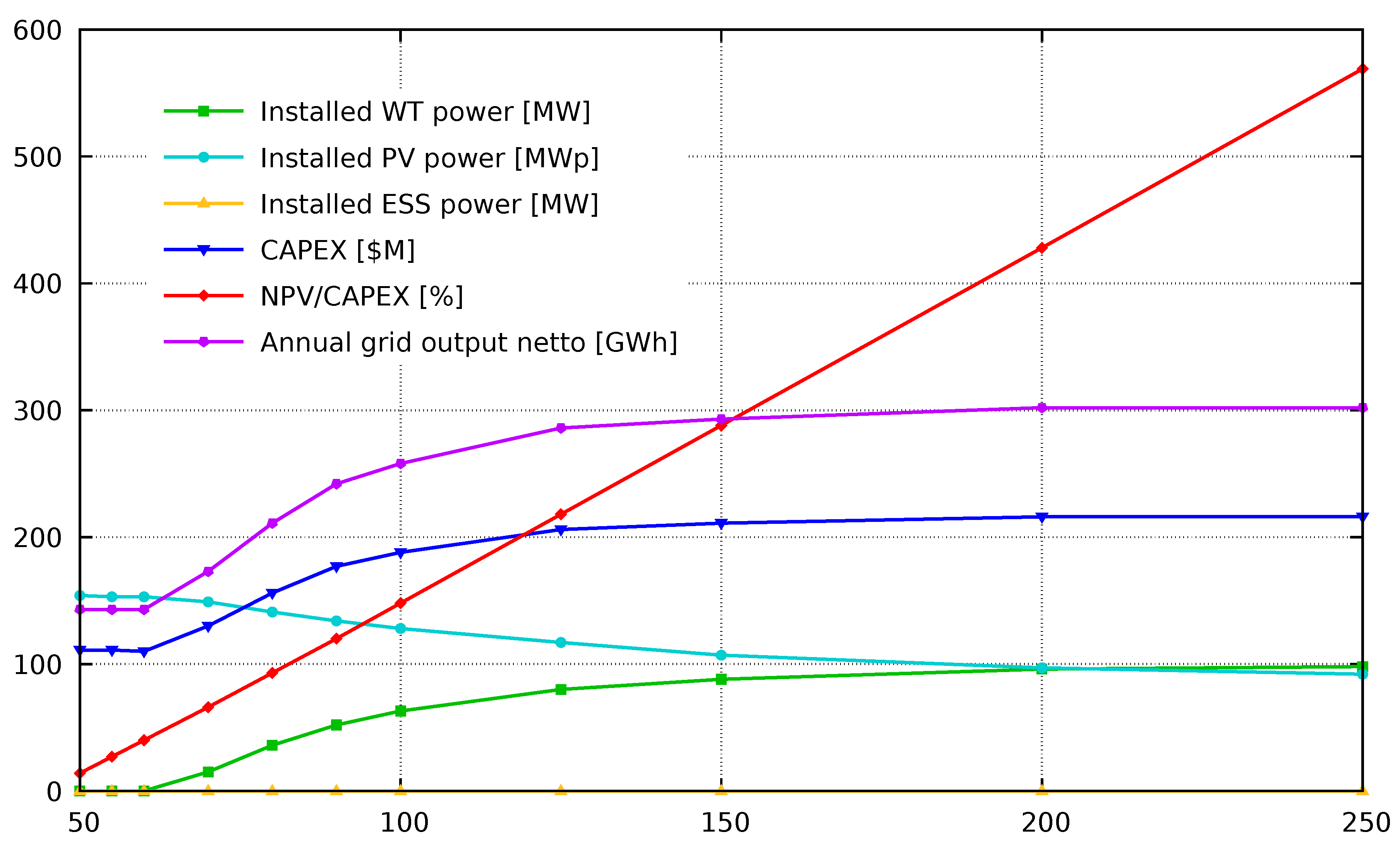
Figure 2.
Case 22 without ESS CAPEX subsidy – calculation results depending on the DAM price multiplier.
Figure 2.
Case 22 without ESS CAPEX subsidy – calculation results depending on the DAM price multiplier.
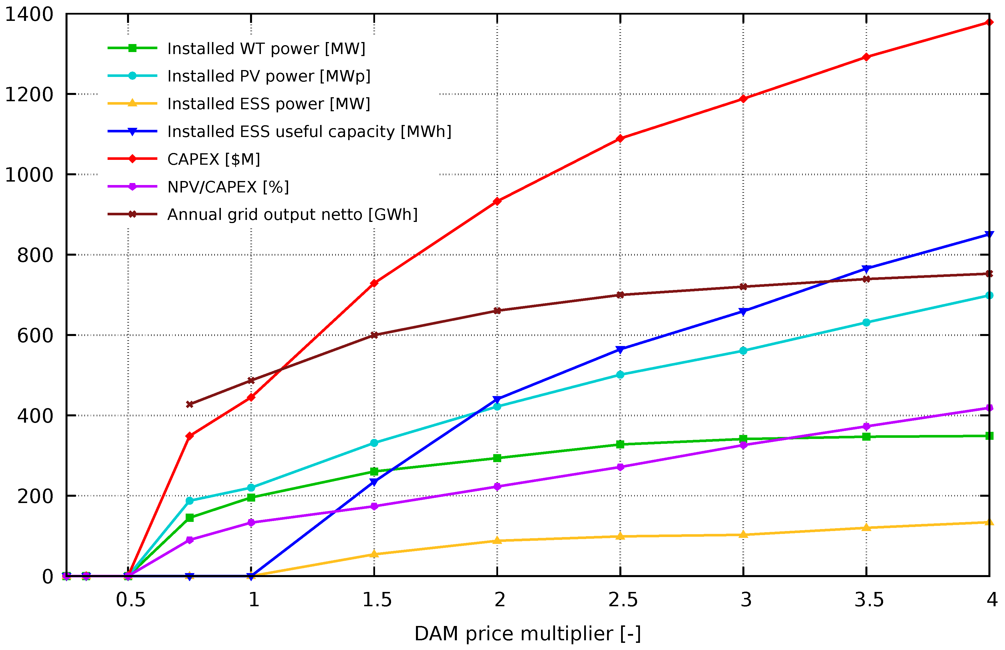
Figure 3.
Case 33 without ESS CAPEX subsidy and with the DAM price multiplier =1.0 – calculation results depending on the CM price.
Figure 3.
Case 33 without ESS CAPEX subsidy and with the DAM price multiplier =1.0 – calculation results depending on the CM price.
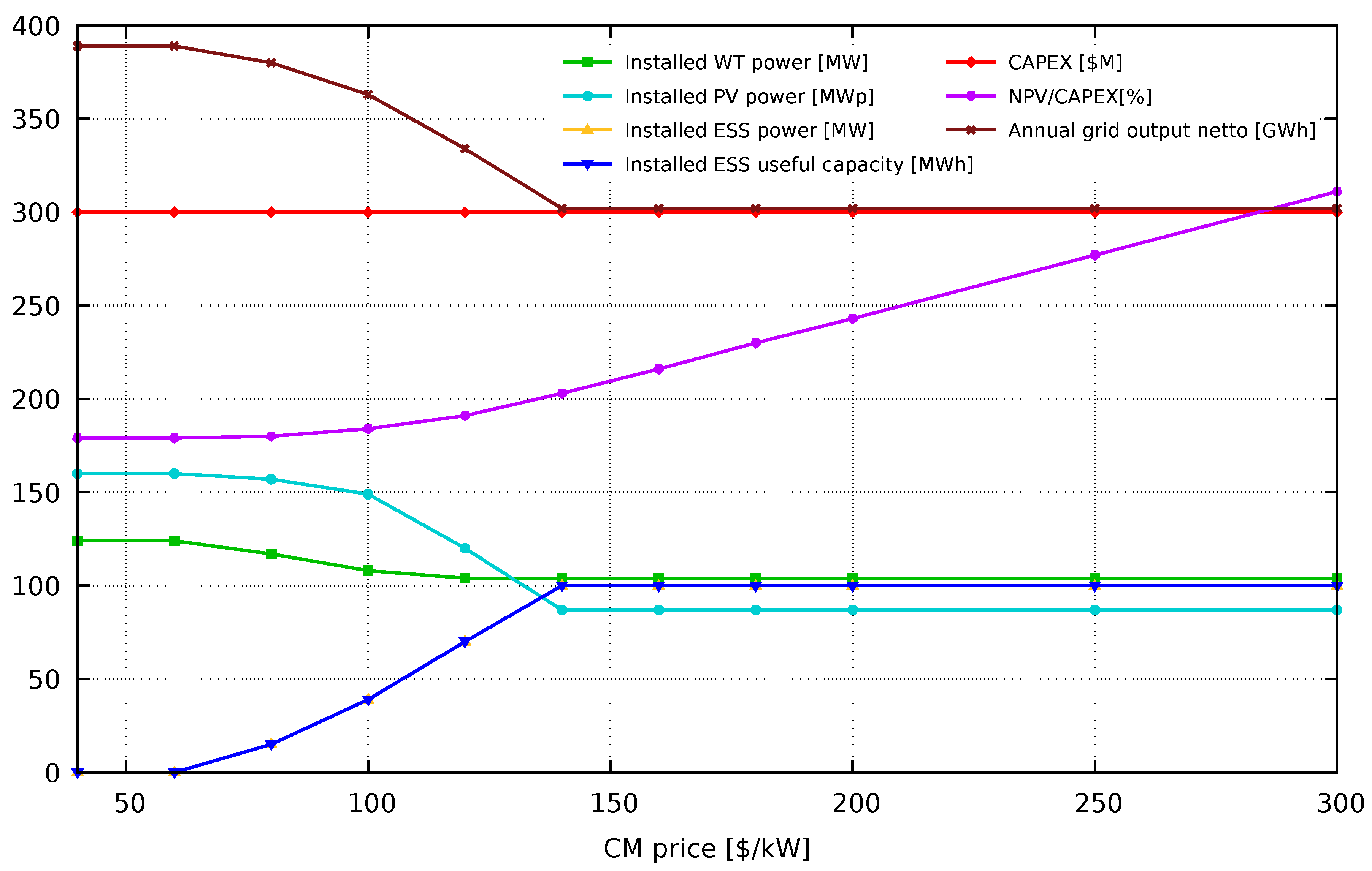
Figure 4.
Optimal composition of sources depending on the financial objective of the investment for DAM.
Figure 4.
Optimal composition of sources depending on the financial objective of the investment for DAM.
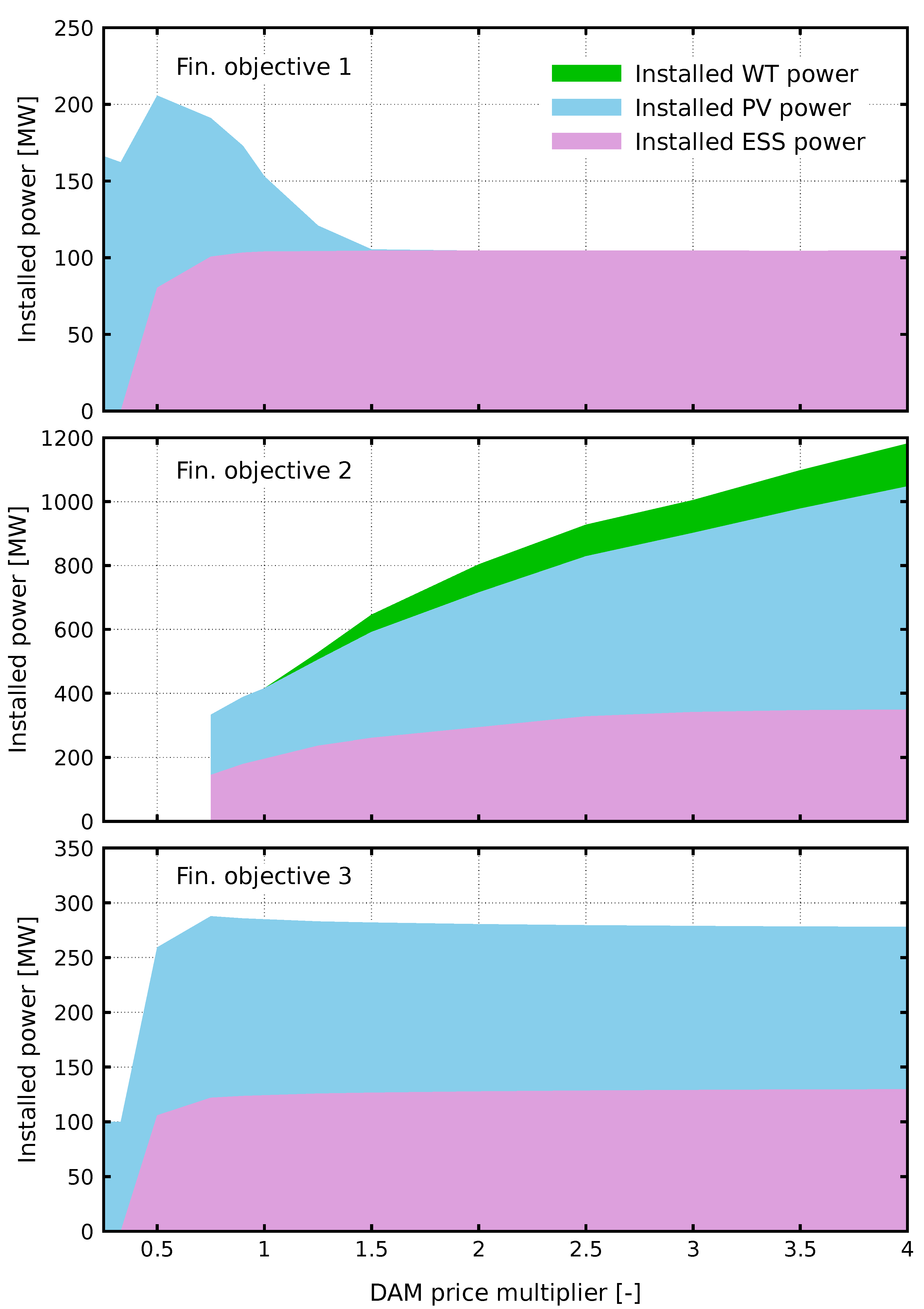
Figure 5.
Optimal composition of sources depending on the source of income and corresponding price level for financial objective 1.
Figure 5.
Optimal composition of sources depending on the source of income and corresponding price level for financial objective 1.
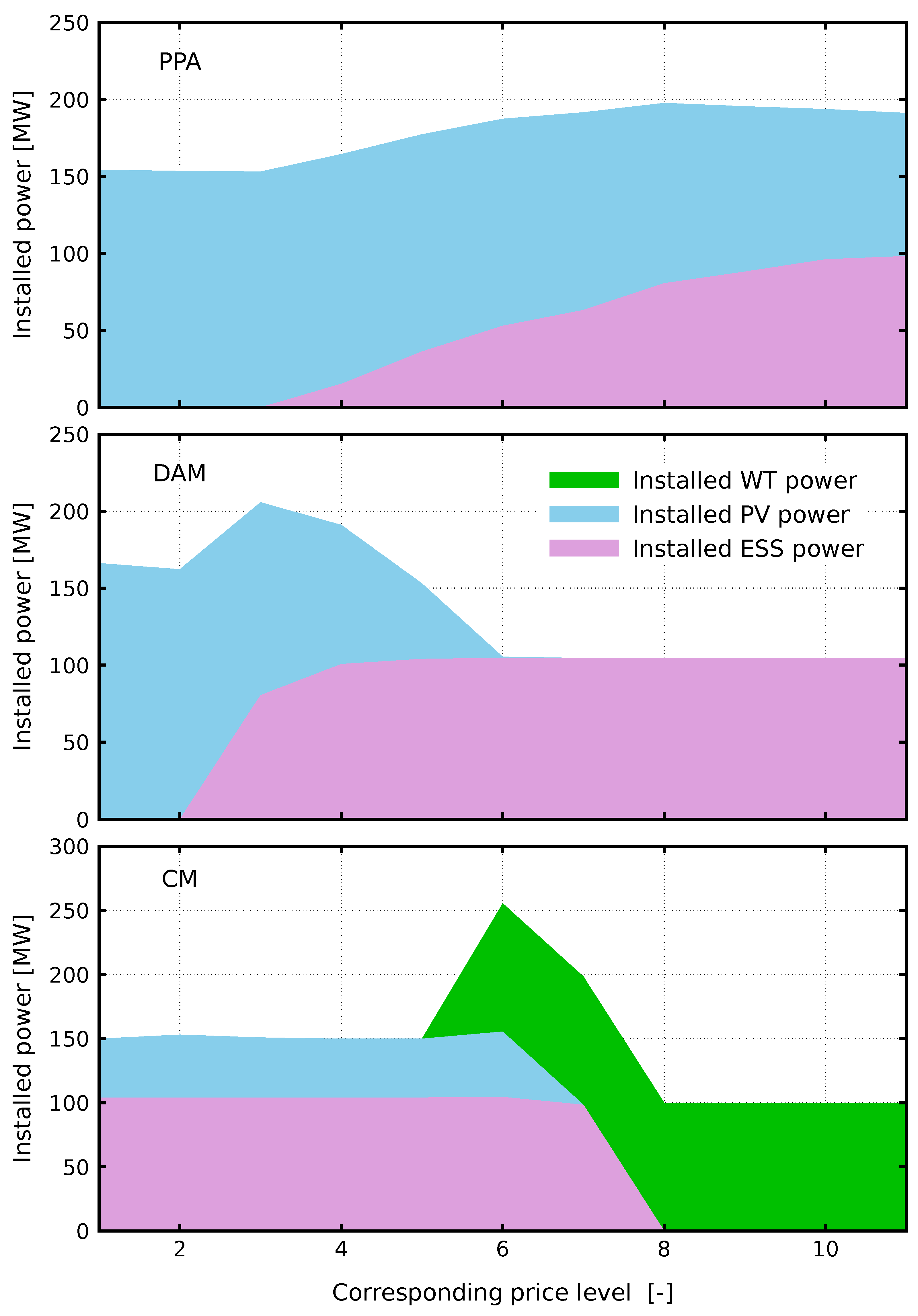
Figure 6.
Optimal composition of sources depending on the DAM price for financial objective 1 and CM.
Figure 6.
Optimal composition of sources depending on the DAM price for financial objective 1 and CM.
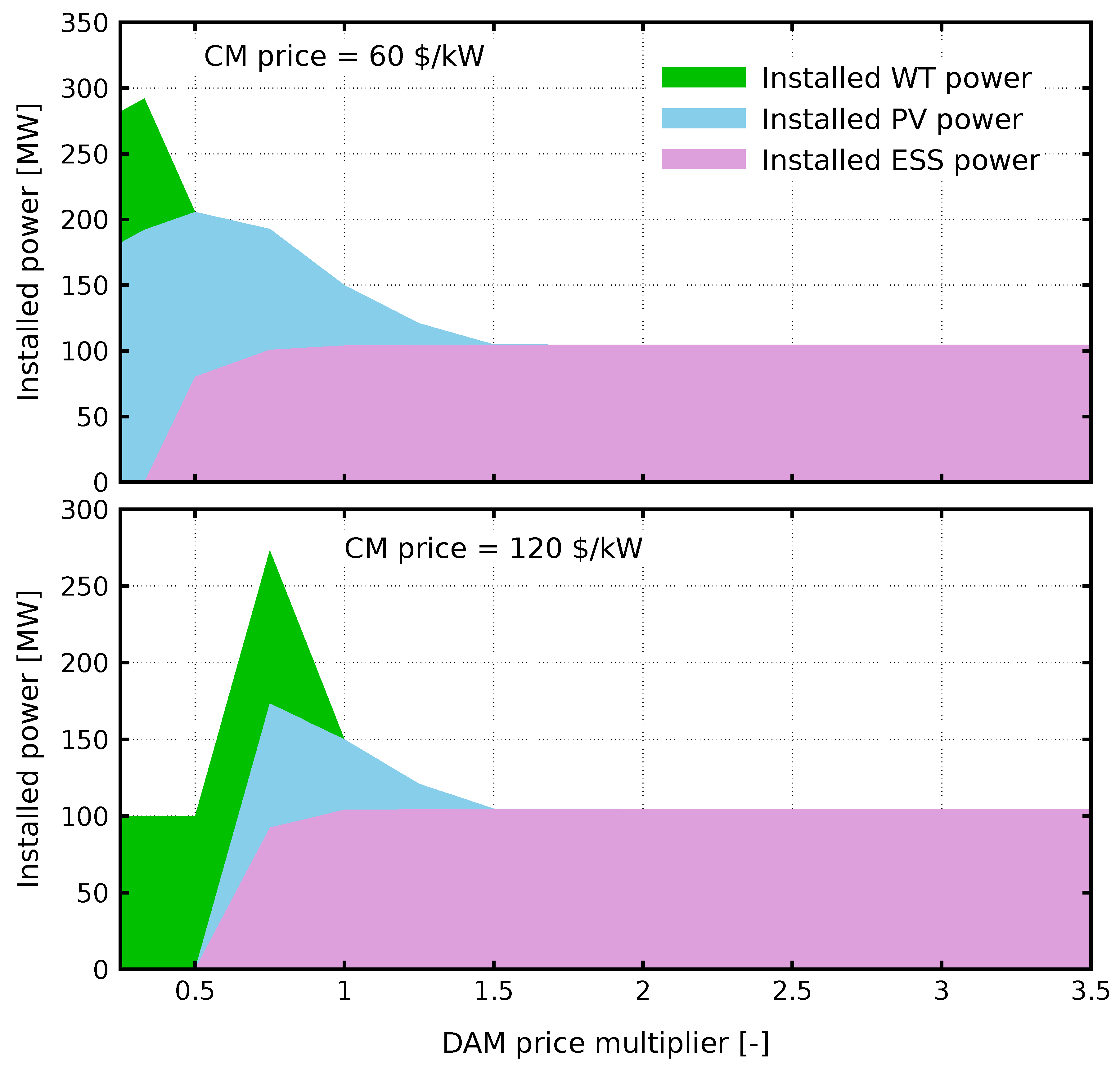
Figure 7.
Optimal composition of sources depending on the ESS CAPEX subsidy for financial objective 2 and the DAM price multiplier = 1.0.
Figure 7.
Optimal composition of sources depending on the ESS CAPEX subsidy for financial objective 2 and the DAM price multiplier = 1.0.
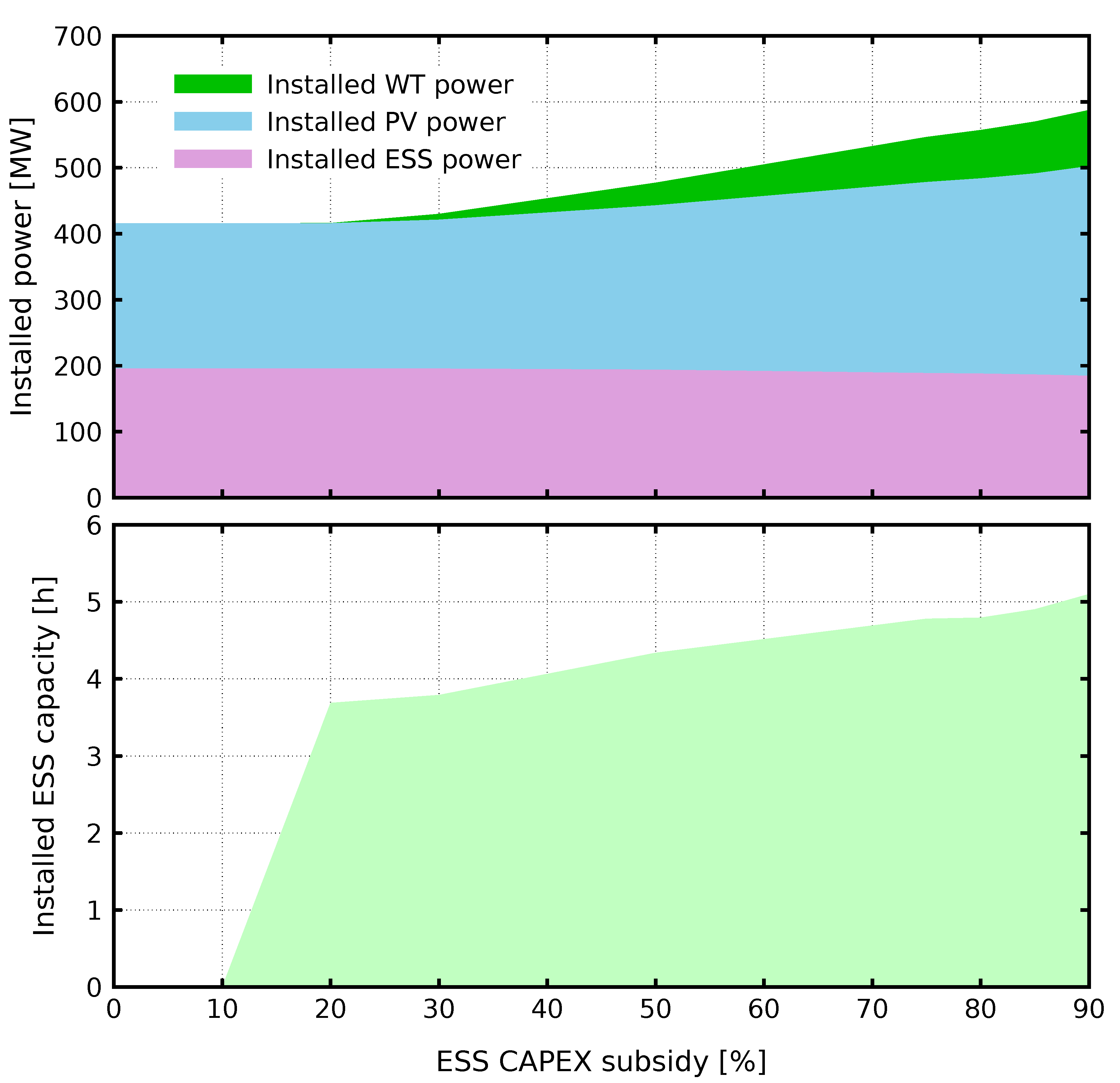
Figure 8.
Single technology NPV and grid output in relation to HRES in Case 12.
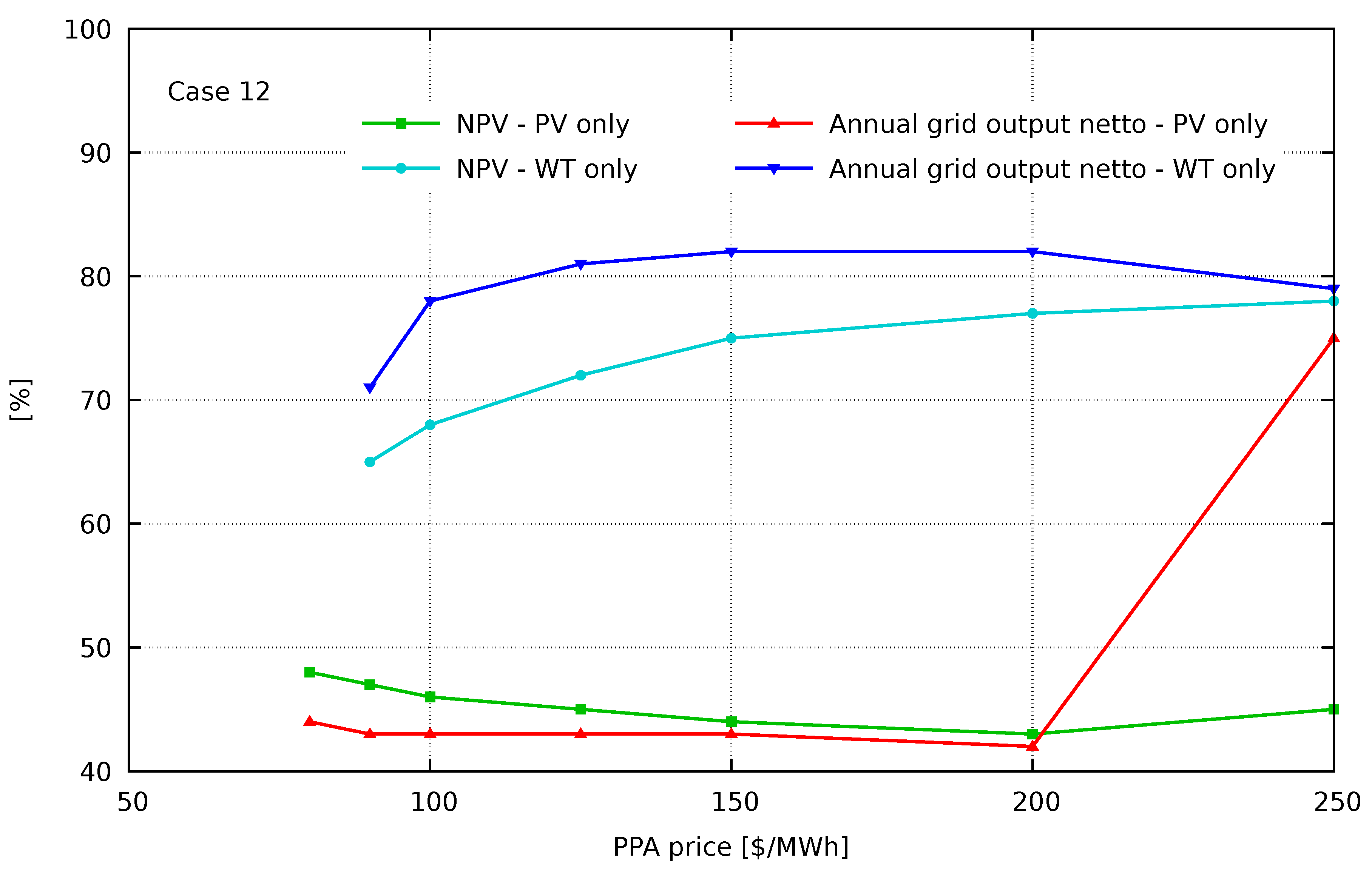
Figure 9.
Single technology NPV and grid output in relation to HRES in Case 23.
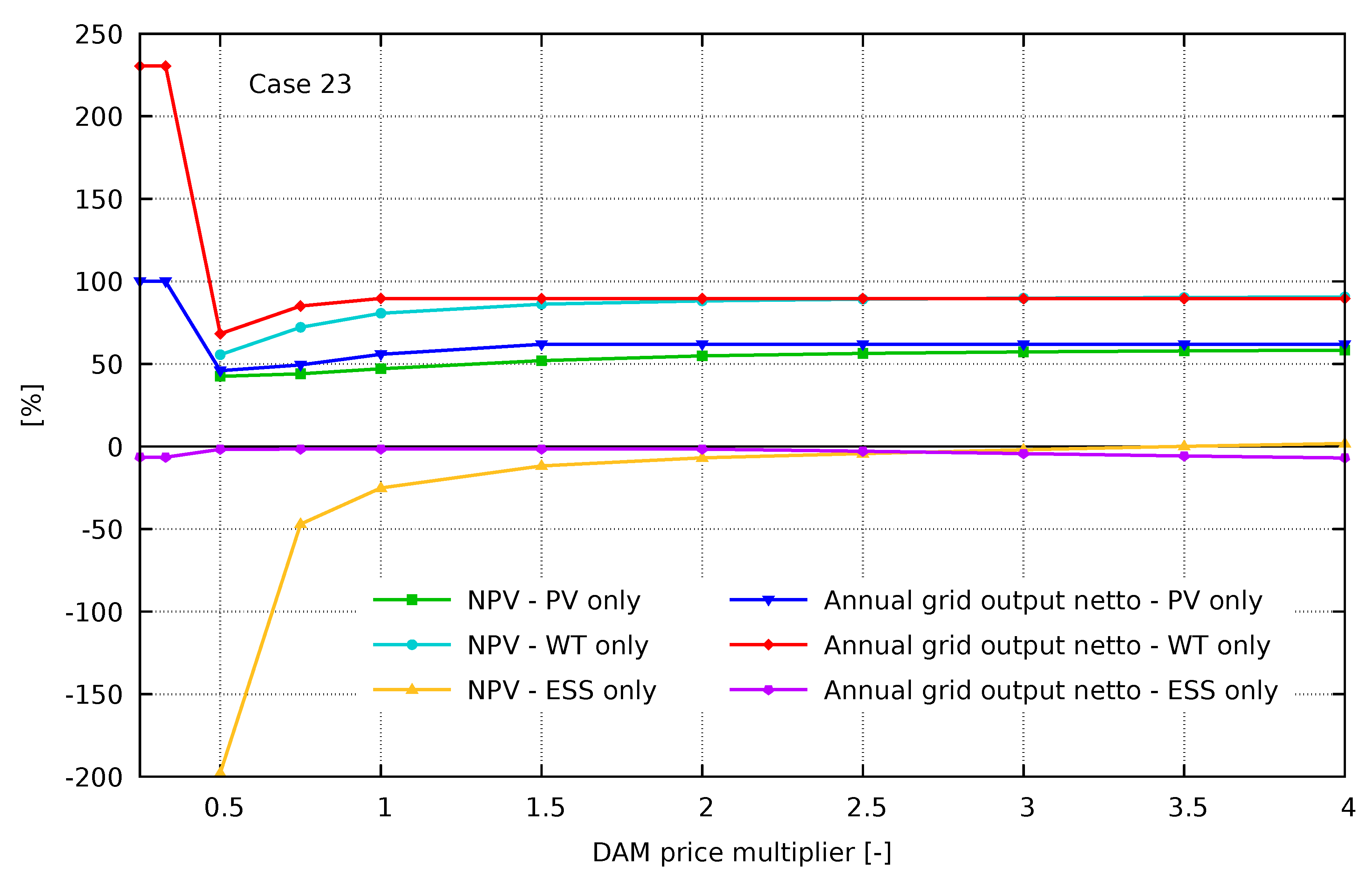

Table 1.
Case 11 without ESS CAPEX subsidy – calculation results depending on the PPA price
| PPA price | [$/MWh] | 50 | 55 | 60 | 70 | 80 | 90 | 100 | 125 | 150 | 200 | 250 |
|---|---|---|---|---|---|---|---|---|---|---|---|---|
| Installed WT power | [MW] | 0.0 | 0.0 | 0.0 | 15.2 | 36.3 | 53.0 | 63.2 | 80.7 | 88.1 | 96.1 | 98.3 |
| Installed PV power | [MWp] | 154.2 | 153.6 | 153.2 | 149.3 | 141.1 | 134.5 | 128.4 | 117.1 | 107.4 | 97.6 | 92.9 |
| Installed ESS power | [MW] | 0.0 | 0.0 | 0.0 | 0.0 | 0.0 | 0.0 | 0.0 | 0.0 | 0.0 | 0.0 | 0.0 |
| CAPEX | [$M] | 111.5 | 111.1 | 110.8 | 130.8 | 156.6 | 177.0 | 188.2 | 206.6 | 211.4 | 216.8 | 216.9 |
| NPV/CAPEX | [%] | 14.1 | 27.1 | 40.1 | 66.3 | 93.3 | 120.8 | 148.4 | 218.1 | 288.1 | 428.6 | 569.3 |
| Annual net grid output | [GWh] | 143.9 | 143.3 | 143.0 | 173.0 | 211.8 | 242.1 | 258.9 | 286.2 | 293.7 | 302.0 | 302.3 |
| RES output reduction | [%] | 1.1 | 1.0 | 1.0 | 0.8 | 0.6 | 0.7 | 0.7 | 0.8 | 0.7 | 0.8 | 0.8 |
| NPV/CAPEX – PV only | [%] | 14.1 | 27.1 | 40.1 | 66.2 | 92.3 | 118.3 | 144.4 | 209.6 | 274.8 | 405.2 | 535.7 |
| NPV/CAPEX – WT only | [%] | -3.3 | 10.8 | 24.9 | 53.1 | 81.4 | 109.6 | 137.8 | 208.4 | 279.0 | 420.1 | 561.3 |
| Annual net grid output – PV only |
[GWh] | 143.8 | 143.3 | 143.0 | 142.3 | 141.7 | 141.2 | 141.0 | 140.5 | 140.2 | 139.5 | 139.2 |
| Annual net grid output – WT only |
[GWh] | 231.8 | 231.7 | 231.7 | 231.6 | 231.4 | 231.3 | 231.2 | 231.1 | 231.0 | 230.9 | 230.9 |
Table 2.
Case 12 without ESS CAPEX subsidy – calculation results depending on the PPA price
| PPA price | [$/MWh] | 50 | 55 | 60 | 70 | 80 | 90 | 100 | 125 | 150 | 200 | 250 |
|---|---|---|---|---|---|---|---|---|---|---|---|---|
| Installed WT power | [MW] | 104.2 | 144.7 | 160.2 | 196.1 | 231.0 | 285.2 | 334.1 | ||||
| Installed PV power | [MWp] | 140.3 | 186.4 | 195.5 | 216.4 | 233.8 | 287.7 | 353.0 | ||||
| Installed ESS power | [MW] | 0.0 | 0.0 | 0.0 | 0.0 | 0.0 | 15.8 | 46.5 | ||||
| Installed ESS capacity | [MWh] | 0.0 | 0.0 | 0.0 | 0.0 | 0.0 | 51.3 | 217.9 | ||||
| CAPEX | [$M] | 256.9 | 347.2 | 376.1 | 443.2 | 506.4 | 648.7 | 842.5 | ||||
| NPV | [$M] | 231.2 | 331.6 | 421.0 | 660.4 | 916.6 | 1,471.7 | 2,092.6 | ||||
| Annual net grid output | [GWh] | 352.0 | 432.7 | 452.9 | 492.8 | 523.4 | 579.9 | 645.3 | ||||
| RES output reduction | [%] | 2.9 | 12.6 | 15.8 | 22.6 | 28.3 | 35.4 | 38.9 | ||||
| NPV – PV only | [$M] | 111.2 | 156.0 | 194.9 | 299.4 | 410.7 | 647.0 | 961.4 | ||||
| NPV – WT only | [$M] | 217.3 | 288.8 | 479.2 | 688.7 | 1,147.4 | 1,648.4 | |||||
| Annual net grid output – PV only |
[GWh] | 157.1 | 189.4 | 196.9 | 215.4 | 225.1 | 244.0 | 488.4 | ||||
| Annual net grid output – WT only |
[GWh] | 310.1 | 353.5 | 399.2 | 429.3 | 476.9 | 514.5 |
Table 3.
Case 13 without ESS CAPEX subsidy – calculation results depending on the PPA price
| PPA price | [$/MWh] | 50 | 55 | 60 | 70 | 80 | 90 | 100 | 125 | 150 | 200 | 250 |
|---|---|---|---|---|---|---|---|---|---|---|---|---|
| Installed WT power | [MW] | 71.9 | 104.0 | 105.7 | 116.4 | 121.1 | 121.9 | 122.5 | 124.1 | 125.1 | 126.2 | 126.8 |
| Installed PV power | [MWp] | 146.9 | 147.8 | 154.7 | 167.2 | 167.7 | 166.1 | 164.6 | 161.0 | 158.7 | 156.4 | 154.9 |
| Installed ESS power | [MW] | 0.0 | 0.0 | 0.0 | 0.0 | 0.0 | 0.0 | 0.0 | 0.0 | 0.0 | 0.0 | 0.0 |
| CAPEX | [$M] | 213.3 | 261.5 | 268.5 | 292.7 | 300.0 | 300.0 | 300.0 | 300.0 | 300.0 | 300.0 | 300.0 |
| NPV | [$M] | 19.7 | 53.8 | 90.1 | 165.9 | 245.3 | 325.0 | 404.8 | 604.3 | 803.9 | 1,203.3 | 1,602.8 |
| Annual net grid output | [GWh] | 291.5 | 356.7 | 363.8 | 387.6 | 394.7 | 394.9 | 395.1 | 395.4 | 395.6 | 395.7 | 395.8 |
| RES output reduction | [%] | 2.0 | 3.4 | 4.1 | 6.5 | 7.3 | 7.2 | 7.2 | 7.2 | 7.1 | 7.1 | 7.1 |
| NPV – PV only | [$M] | 16.2 | 31.9 | 48.2 | 82.4 | 118.5 | 156.0 | 194.9 | 299.4 | 410.7 | 647.0 | 891.9 |
| NPV – WT only | [$M] | -28.4 | -5.5 | 18.1 | 42.6 | 95.8 | 154.8 | 219.4 | 288.8 | 468.1 | 647.4 | 1,006.1 |
| Annual net grid output – PV only |
[GWh] | 152.7 | 158.1 | 164.6 | 174.1 | 182.8 | 189.4 | 196.9 | 215.4 | 225.1 | 242.7 | 242.7 |
| Annual net grid output – WT only |
[GWh] | 220.8 | 230.8 | 236.8 | 250.1 | 277.5 | 306.5 | 332.8 | 353.5 | 355.3 | 355.3 | 355.3 |
Table 4.
Case 21 without ESS CAPEX subsidy – calculation results on the DAM price multiplier
| DAM price multiplier | [-] | 0.25 | 0.33 | 0.5 | 0.75 | 1.0 | 1.5 | 2.0 | 2.5 | 3.0 | 3.5 | 4.0 |
|---|---|---|---|---|---|---|---|---|---|---|---|---|
| Installed WT power | [MW] | 0.0 | 0.0 | 80.4 | 100.7 | 104.0 | 104.6 | 104.6 | 104.6 | 104.6 | 104.5 | 104.6 |
| Installed PV power | [MWp] | 166.2 | 162.2 | 125.3 | 90.4 | 49.0 | 0.8 | 0.0 | 0.0 | 0.0 | 0.0 | 0.0 |
| Installed ESS power | [MW] | 0.0 | 0.0 | 0.0 | 0.0 | 0.0 | 0.0 | 0.0 | 0.0 | 0.0 | 0.0 | 0.0 |
| CAPEX | [$M] | 119.4 | 116.7 | 211.7 | 218.8 | 196.5 | 165.6 | 165.1 | 165.1 | 165.1 | 165.0 | 165.1 |
| NPV/CAPEX | [%] | -44.6 | -21.8 | 30.8 | 112.6 | 195.5 | 364.2 | 533.7 | 703.3 | 872.8 | 1,042.4 | 1,211.9 |
| Annual net grid output | [GWh] | 152.0 | 149.1 | 288.2 | 299.9 | 269.8 | 226.7 | 225.9 | 225.9 | 225.9 | 225.9 | 226.0 |
| RES output reduction | [%] | 3.1 | 2.5 | 2.6 | 2.5 | 2.2 | 2.1 | 2.1 | 2.1 | 2.1 | 2.1 | 2.1 |
| NPV/CAPEX – PV only | [%] | -44.6 | -21.8 | 26.7 | 98.0 | 169.4 | 312.2 | 455.1 | 597.9 | 740.7 | 883.6 | 915.7 |
| NPV/CAPEX – WT only | [%] | -59.7 | -32.6 | 25.1 | 109.8 | 194.6 | 364.2 | 533.7 | 703.3 | 872.8 | 1,042.4 | 1,211.9 |
| Annual net grid output – PV only |
[GWh] | 152.0 | 149.1 | 146.3 | 144.9 | 144.0 | 142.9 | 142.2 | 141.9 | 141.7 | 141.6 | 141.5 |
| Annual net grid output – WT only |
[GWh] | 227.8 | 227.0 | 226.7 | 226.3 | 226.1 | 226.0 | 225.9 | 225.9 | 225.9 | 225.9 | 226.0 |
Table 5.
Case 22 without ESS CAPEX subsidy – calculation results depending on the DAM price multiplier
Table 5.
Case 22 without ESS CAPEX subsidy – calculation results depending on the DAM price multiplier
| DAM price multiplier | [-] | 0.25 | 0.33 | 0.5 | 0.75 | 1.0 | 1.5 | 2.0 | 2.5 | 3.0 | 3.5 | 4.0 |
|---|---|---|---|---|---|---|---|---|---|---|---|---|
| Installed WT power | [MW] | 145.2 | 195.6 | 260.4 | 293.7 | 327.7 | 341.2 | 346.9 | 348.9 | |||
| Installed PV power | [MWp] | 187.5 | 220.1 | 331.6 | 422.0 | 501.3 | 561.0 | 631.4 | 698.9 | |||
| Installed ESS power | [MW] | 0.0 | 0.0 | 54.2 | 87.9 | 98.8 | 102.7 | 120.1 | 134.1 | |||
| Installed ESS useful capacity | [MWh] | 0.0 | 0.0 | 235.0 | 440.5 | 564.6 | 659.3 | 765.6 | 850.9 | |||
| CAPEX | [$M] | 348.8 | 444.9 | 729.0 | 932.9 | 1,089.4 | 1,188.1 | 1,292.1 | 1,378.9 | |||
| NPV | [$M] | 313.9 | 592.4 | 1,266.8 | 2,078.6 | 2,957.7 | 3,874.2 | 4,815.7 | 5,775.7 | |||
| Annual net grid output | [GWh] | 427.5 | 486.9 | 599.8 | 660.6 | 699.9 | 720.4 | 739.4 | 752.8 | |||
| RES output reduction | [%] | 14.1 | 23.9 | 31.1 | 34.9 | 39.6 | 41.9 | 43.7 | 45.4 | |||
| NPV – PV only | [$M] | 130.4 | 253.6 | 522.8 | 825.5 | 1,154.3 | 1,499.6 | 1,855.9 | 2,222.5 | |||
| NPV – WT only | [$M] | 218.2 | 444.0 | 973.4 | 1,573.1 | 2,218.7 | 2,899.9 | 3,608.4 | 4,337.1 | |||
| Annual net grid output – PV only |
[GWh] | 174.5 | 217.4 | 242.5 | 265.7 | 280.3 | 288.8 | 295.7 | 303.4 | |||
| Annual net grid output – WT only |
[GWh] | 305.1 | 389.6 | 459.5 | 504.0 | 534.2 | 559.0 | 577.4 | 591.0 |
Table 6.
Case 23 without ESS CAPEX subsidy – calculation results depending on the DAM price multiplier
Table 6.
Case 23 without ESS CAPEX subsidy – calculation results depending on the DAM price multiplier
| DAM price multiplier | [-] | 0.25 | 0.33 | 0.5 | 0.75 | 1.0 | 1.5 | 2.0 | 2.5 | 3.0 | 3.5 | 4.0 |
|---|---|---|---|---|---|---|---|---|---|---|---|---|
| Installed WT power | [MW] | 0.0 | 0.0 | 105.9 | 122.0 | 124.2 | 126.6 | 127.8 | 128.6 | 129.1 | 129.5 | 129.7 |
| Installed PV power | [MWp] | 100.0 | 100.0 | 153.4 | 165.8 | 160.8 | 155.4 | 152.7 | 151.0 | 149.8 | 148.8 | 148.5 |
| Installed ESS power | [MW] | 0.0 | 0.0 | 0.0 | 0.0 | 0.0 | 0.0 | 0.0 | 0.0 | 0.0 | 0.0 | 0.0 |
| CAPEX | [$M] | 75.8 | 75.8 | 268.0 | 300.0 | 300.0 | 300.0 | 300.0 | 300.0 | 300.0 | 300.0 | 300.0 |
| NPV | [$M] | -39.0 | -22.4 | 77.0 | 305.8 | 538.8 | 1,005.4 | 1,472.2 | 1,939.1 | 2,406.1 | 2,873.2 | 3,340.2 |
| Annual net grid output | [GWh] | 93.8 | 93.8 | 357.9 | 388.9 | 389.4 | 389.7 | 389.8 | 389.8 | 389.9 | 389.9 | 389.8 |
| RES output reduction | [%] | 0.6 | 0.6 | 5.4 | 8.6 | 8.6 | 8.5 | 8.5 | 8.5 | 8.5 | 8.6 | 8.6 |
| NPV – PV only | [$M] | -39.0 | -22.4 | 32.7 | 134.6 | 253.6 | 522.7 | 807.9 | 1,093.2 | 1,378.4 | 1,663.6 | 1,948.8 |
| NPV – WT only | [$M] | -95.1 | -52.3 | 42.8 | 220.7 | 434.7 | 866.4 | 1,298.0 | 1,729.6 | 2,161.2 | 2,592.9 | 3,024.5 |
| NPV – ESS only | [$M] | -160.8 | -158.1 | -152.3 | -143.8 | -135.3 | -118.3 | -101.2 | -83.5 | -47.1 | 2.7 | 60.5 |
| Annual net grid output – PV only |
[GWh] | 93.8 | 93.8 | 164.3 | 192.1 | 217.4 | 241.2 | 241.2 | 241.2 | 241.2 | 241.2 | 241.2 |
| Annual net grid output – WT only |
[GWh] | 216.1 | 216.1 | 244.3 | 330.8 | 349.2 | 349.2 | 349.2 | 349.2 | 349.2 | 349.2 | 349.2 |
| Annual net grid output – ESS only |
[GWh] | -6.1 | -6.1 | -6.1 | -6.1 | -6.1 | -6.1 | -6.1 | -11.2 | -16.8 | -22.4 | -27.1 |
Table 7.
Case 31 without ESS CAPEX subsidy and with the DAM price multiplier =1.0 – calculation results depending on the CM price
Table 7.
Case 31 without ESS CAPEX subsidy and with the DAM price multiplier =1.0 – calculation results depending on the CM price
| CM price | [$/kW] | 40 | 60 | 80 | 100 | 120 | 140 | 160 | 180 | 200 | 250 | 300 |
|---|---|---|---|---|---|---|---|---|---|---|---|---|
| Installed WT power | [MW] | 104.0 | 104.0 | 104.0 | 104.0 | 104.0 | 104.5 | 98.4 | 0.0 | 0.0 | 0.0 | 0.0 |
| Installed PV power | [MWp] | 45.9 | 49.0 | 46.8 | 45.9 | 45.9 | 50.9 | 0.0 | 0.0 | 0.0 | 0.0 | 0.0 |
| Installed ESS power | [MW] | 0.0 | 0.0 | 0.0 | 0.0 | 0.0 | 100.0 | 100.0 | 100.0 | 100.0 | 100.0 | 100.0 |
| Installed WT power | [MWh] | 0.0 | 0.0 | 0.0 | 0.0 | 0.0 | 100.0 | 100.0 | 100.0 | 100.0 | 100.0 | 100.0 |
| CAPEX | [$M] | 194.5 | 196.5 | 195.1 | 194.5 | 194.5 | 276.2 | 233.6 | 87.7 | 87.7 | 87.7 | 87.7 |
| NPV/CAPEX | [%] | 195.5 | 195.5 | 195.5 | 195.5 | 195.5 | 203.7 | 219.5 | 248.6 | 306.1 | 421.2 | 536.3 |
| Annual net grid output | [GWh] | 267.0 | 269.8 | 267.8 | 267.0 | 267.0 | 268.8 | 207.6 | -6.1 | -6.1 | -6.1 | -6.1 |
| RES output reduction | [%] | 2.2 | 2.2 | 2.2 | 2.2 | 2.2 | 1.7 | 2.0 | 0.0 | 0.0 | 0.0 | 0.0 |
| NPV/CAPEX – PV only | [%] | 169.4 | 169.4 | 169.4 | 169.4 | 169.4 | 169.4 | 169.4 | 169.4 | 169.4 | 169.4 | 169.4 |
| NPV/CAPEX – WT only | [%] | 194.6 | 194.6 | 194.6 | 194.6 | 194.6 | 194.6 | 194.6 | 194.6 | 194.6 | 194.6 | 194.6 |
| NPV/CAPEX – ESS only | [%] | -54.5 | -14.2 | 26.2 | 66.6 | 107.0 | 147.3 | 187.7 | 228.1 | 268.5 | 369.4 | 470.4 |
| Annual net grid output – PV only |
[GWh] | 144.0 | 144.0 | 144.0 | 144.0 | 144.0 | 144.0 | 144.0 | 144.0 | 144.0 | 144.0 | 144.0 |
| Annual net grid output – WT only |
[GWh] | 226.1 | 226.1 | 226.1 | 226.1 | 226.1 | 226.1 | 226.1 | 226.1 | 226.1 | 226.1 | 226.1 |
| Annual net grid output – ESS only |
[GWh] | -6.1 | -6.1 | -6.1 | -6.1 | -6.1 | -6.1 | -6.1 | -6.1 | -6.1 | -6.1 | -6.1 |
Table 8.
Case 32 without ESS CAPEX subsidy and with the DAM price multiplier = 1.0 – calculation results depending on the CM price
Table 8.
Case 32 without ESS CAPEX subsidy and with the DAM price multiplier = 1.0 – calculation results depending on the CM price
| CM price | [$/kW] | 40 | 60 | 80 | 100 | 120 | 140 | 160 | 1 80 | 200 | 250 | 300 |
|---|---|---|---|---|---|---|---|---|---|---|---|---|
| Installed WT power | [MW] | 196.5 | 196.5 | 196.5 | 196.5 | 196.5 | 196.5 | 196.5 | 196.5 | 196.5 | 196.5 | 196.5 |
| Installed PV power | [MWp] | 239.6 | 239.6 | 239.6 | 239.6 | 239.6 | 239.6 | 239.6 | 239.6 | 239.6 | 239.6 | 239.6 |
| Installed ESS power | [MW] | 100.0 | 100.0 | 100.0 | 100.0 | 100.0 | 100.0 | 100.0 | 100.0 | 100.0 | 100.0 | 100.0 |
| Installed WT power | [MWh] | 100.0 | 100.0 | 100.0 | 100.0 | 100.0 | 100.0 | 100.0 | 100.0 | 100.0 | 100.0 | 100.0 |
| CAPEX | [$M] | 536.8 | 536.8 | 536.8 | 536.8 | 536.8 | 536.8 | 536.8 | 536.8 | 536.8 | 536.8 | 536.8 |
| NPV | [$M] | 608.1 | 648.5 | 688.9 | 729.2 | 769.6 | 810.0 | 850.4 | 890.7 | 931.1 | 1,032.1 | 1,133.0 |
| Annual net grid output | [GWh] | 514.5 | 514.5 | 514.5 | 514.5 | 514.5 | 514.5 | 514.5 | 514.5 | 514.5 | 514.5 | 514.5 |
| RES output reduction | [%] | 21.3 | 21.3 | 21.3 | 21.3 | 21.3 | 21.3 | 21.3 | 21.3 | 21.3 | 21.3 | 21.3 |
| NPV – PV only | [$M] | 608.1 | 648.5 | 688.9 | 729.2 | 769.6 | 810.0 | 850.4 | 890.7 | 931.1 | 1,032.1 | 1,133.0 |
| NPV – WT only | [$M] | 444.0 | 444.0 | 444.0 | 444.0 | 444.0 | 444.0 | 444.0 | 444.0 | 444.0 | 444.0 | 444.0 |
| NPV – ESS only | [$M] | 107.0 | 147.3 | 187.7 | 228.1 | 268.5 | 369.4 | 470.4 | ||||
| Annual net grid output – PV only |
[GWh] | 217.4 | 217.4 | 217.4 | 217.4 | 217.4 | 217.4 | 217.4 | 217.4 | 217.4 | 217.4 | 217.4 |
| Annual net grid output – WT only |
[GWh] | 389.6 | 389.6 | 389.6 | 389.6 | 389.6 | 389.6 | 389.6 | 389.6 | 389.6 | 389.6 | 389.6 |
| Annual net grid output – ESS only |
[GWh] | -6.1 | -6.1 | -6.1 | -6.1 | -6.1 | -6.1 | -6.1 |
Table 9.
Case 33 without ESS CAPEX subsidy and with the DAM price multiplier =1.0 – calculation results depending on the CM price
Table 9.
Case 33 without ESS CAPEX subsidy and with the DAM price multiplier =1.0 – calculation results depending on the CM price
| CM price | [$/kW] | 40 | 60 | 80 | 100 | 120 | 140 | 160 | 180 | 200 | 250 | 300 |
|---|---|---|---|---|---|---|---|---|---|---|---|---|
| Installed WT power | [MW] | 124.2 | 124.2 | 117.3 | 109.0 | 104.8 | 104.2 | 104.2 | 104.2 | 104.2 | 104.2 | 104.2 |
| Installed PV power | [MWp] | 160.8 | 160.8 | 157.4 | 149.0 | 120.8 | 87.7 | 87.7 | 87.7 | 87.7 | 87.7 | 87.7 |
| Installed ESS power | [MW] | 0.0 | 0.0 | 15.9 | 39.0 | 70.8 | 100.0 | 100.0 | 100.0 | 100.0 | 100.0 | 100.0 |
| Installed WT power | [MWh] | 0.0 | 0.0 | 15.9 | 39.0 | 70.8 | 100.0 | 100.0 | 100.0 | 100.0 | 100.0 | 100.0 |
| CAPEX | [$M] | 300.0 | 300.0 | 300.0 | 300.0 | 300.0 | 300.0 | 300.0 | 300.0 | 300.0 | 300.0 | 300.0 |
| NPV | [$M] | 538.8 | 538.8 | 538.8 | 541.5 | 552.2 | 574.0 | 610.4 | 650.7 | 691.1 | 731.5 | 832.4 |
| Annual net grid output | [GWh] | 389.4 | 389.4 | 380.7 | 363.7 | 334.2 | 302.3 | 302.3 | 302.3 | 302.3 | 302.3 | 302.3 |
| RES output reduction | [%] | 8.6 | 8.6 | 6.4 | 4.1 | 2.2 | 1.7 | 1.7 | 1.7 | 1.7 | 1.7 | 1.7 |
| NPV – PV only | [$M] | 253.6 | 253.6 | 253.6 | 253.6 | 253.6 | 253.6 | 253.6 | 253.6 | 253.6 | 253.6 | 253.6 |
| NPV – WT only | [$M] | 434.7 | 434.7 | 434.7 | 434.7 | 434.7 | 434.7 | 434.7 | 434.7 | 434.7 | 434.7 | 434.7 |
| NPV – ESS only | [$M] | -54.5 | -14.2 | 26.2 | 66.6 | 107.0 | 147.3 | 187.7 | 228.1 | 268.5 | 369.4 | 470.4 |
| Annual net grid output – PV only |
[GWh] | 217.4 | 217.4 | 217.4 | 217.4 | 217.4 | 217.4 | 217.4 | 217.4 | 217.4 | 217.4 | 217.4 |
| Annual net grid output – WT only |
[GWh] | 349.2 | 349.2 | 349.2 | 349.2 | 349.2 | 349.2 | 349.2 | 349.2 | 349.2 | 349.2 | 349.2 |
| Annual net grid output – ESS only |
[GWh] | -6.1 | -6.1 | -6.1 | -6.1 | -6.1 | -6.1 | -6.1 | -6.1 | -6.1 | -6.1 | -6.1 |
Disclaimer/Publisher’s Note: The statements, opinions and data contained in all publications are solely those of the individual author(s) and contributor(s) and not of MDPI and/or the editor(s). MDPI and/or the editor(s) disclaim responsibility for any injury to people or property resulting from any ideas, methods, instructions or products referred to in the content. |
© 2025 by the authors. Licensee MDPI, Basel, Switzerland. This article is an open access article distributed under the terms and conditions of the Creative Commons Attribution (CC BY) license (http://creativecommons.org/licenses/by/4.0/).
Copyright: This open access article is published under a Creative Commons CC BY 4.0 license, which permit the free download, distribution, and reuse, provided that the author and preprint are cited in any reuse.


