Submitted:
08 November 2024
Posted:
12 November 2024
You are already at the latest version
Abstract
This article proposes a two-stage sequential configuration method for energy storage systems to solve the problems of heavy load, low voltage, and increased network loss caused by the large number of electric vehicle (EV) charging piles and distributed photovoltaic (PV) access in urban old and unbalanced distribution networks. In the stage of selecting the location of energy storage, a comprehensive power flow sensitivity variance (CPFSV) is defined to determine the location of energy storage; In the energy storage capacity configuration stage, the energy storage capacity is optimized by considering the benefits of peak shaving and valley filling, energy storage costs, and distribution network voltage deviations. Finally, simulations were conducted using a modified IEEE-33-node system, and the results obtained using the improved Beluga whale optimization algorithm showed that the peak-to-valley difference of the system after the addition of energy storage decreased by 43.7% and 51.1% compared to the original system and the system with EV and PV resources added, respectively. The maximum CPFSV of the system decreased by 52% and 75.1%, respectively; In addition, the engineering value of this method was verified through a real-machine system with 199 nodes in a district of Kunming. Therefore, the energy storage configuration method proposed in this article can provide a reference for solving the outstanding problems caused by the large-scale access of EVs and PVs to the distribution network.
Keywords:
energy storage site selection and capacity determination
; distribution network
; comprehensive power flow sensitivity variance
; beluga whale optimization algorithm
; electric vehicles
; photovoltaic consumption
1. Introduction
In China, in order to reduce carbon dioxide emissions, industries such as electric vehicles and photovoltaics have developed rapidly. The proportion of private EV charging stations and PV connected to urban distribution networks has been increasing year by year, making problems such as insufficient power supply, undervoltage, heavy load, and three-phase imbalance more prominent [1,2,3]. In addition, due to factors such as insufficient space for upgrading and renovating old distribution networks in some urban areas and poor economic efficiency, these problems have been difficult to effectively solve. At present, the commonly used solution is to improve the stability and flexibility of the power grid by decoupling the production and usage time of electricity through Distributed Energy Storage Systems (DESS)[4]. In many regions, it is stipulated that the proportion of energy storage configuration in the distribution network should not be less than 10%. However, the access location and capacity ratio of DESS are closely related to the safe and stable operation of the distribution network, and the cost of DESS is high. Therefore, it is particularly important to optimize the location and capacity of DESS reasonably [5].
At present, there are many studies on the location and capacity of energy storage in distribution networks. Based on system economy and stability, literature [6] considers energy storage costs and adopts a two-layer optimization model to optimize the configuration of DESS. Reference [7] proposes a dual layer configuration method for DESS based on price demand response, which significantly reduces total operating costs and improves system reliability. In response to the problem of poor distribution network vulnerability caused by large-scale distributed power grid integration, reference [8] establishes a two-layer optimization configuration method based on IDEC-K cluster, considering the economy and reliability of DPV and ESS. This method can reduce the voltage fluctuation range of each node in the distribution network, lower the risk of voltage exceeding the limit and line loss rate of the distribution network. The method of dual layer planning of energy storage location and capacity adopted in the above literature is prone to falling into the curse of dimensionality. In contrast, the sequential configuration of location capacity does not have this issue.
In response, reference [9] proposed a three-layer sequential planning method for energy storage location capacity, introducing voltage violation risk coefficient to select the location of DESS, considering investment cost, residual value of DESS, and system operating cost to obtain the optimal capacity of DESS. Reference [10] defines a network loss sensitivity variance to select the location of energy storage access to the distribution network, optimizes the charging and discharging power of energy storage with line loss and bus voltage fluctuations as the objective function, and determines the optimal capacity of energy, effectively reducing the degree of network loss and voltage fluctuations in the distribution network. Reference [11] proposes an energy storage optimization configuration method for the reverse distribution of new energy in the substation area. Firstly, an economic model for optimizing the energy storage capacity in the substation area is established, and then comprehensive indicators such as economy and reliability are considered to select the energy storage site. This method can effectively balance the economy of energy storage investment and the reliability of the power grid. The above literature overcomes the problem of dimensionality disaster, but does not consider the three-phase imbalance of actual distribution networks, and cannot effectively solve the problem of low voltage in distribution networks.
Regarding the energy storage configuration of three-phase unbalanced networks, reference [12] focuses on the three-phase balance caused by asymmetric random access of distributed power sources to the distribution network. A comprehensive direct power flow algorithm for unbalanced active distribution networks is proposed to calculate the power flow problem of unbalanced active distribution networks. Reference [13] proposes a two-stage hybrid optimization configuration model for unbalanced active distribution network DESS considering source load uncertainty. In the first stage, the DESS configuration capacity is optimized to reduce investment and maintenance costs. In the second stage, the DESS charging and discharging plan is optimized to reduce network losses and increase peak shaving and valley filling benefits. The energy storage capacity configured by this method can effectively solve the three-phase imbalance problem of the distribution network. Reference [14] defined a comprehensive loss reduction sensitivity index, considering the impact of DESS charging and discharging on system network loss, and established a multi-objective function to optimize the DESS configuration of unbalanced distribution network. The above literature solves the energy storage configuration problem of three-phase unbalanced networks, but all ignore the management capability of DESS for distribution network voltage. In this regard, reference [15] defined the comprehensive voltage sensitivity variance to select the location of DESS access to unbalanced distribution networks. The configured energy storage has strong voltage management capabilities for unbalanced distribution networks, but this method is only applicable to active distribution networks and is not suitable for urban old distribution networks with a large number of distributed resource access. It also ignores the benefits of DESS in improving load characteristics, peak valley electricity price arbitrage, and other aspects.
It is necessary to study a configuration method for the location and capacity of Distributed Energy Resources (DESS) that is suitable for urban unbalanced distribution networks, as the integration of a large number of Distributed Energy Resources (DERs) brings a series of problems to the old and unbalanced distribution networks in cities. The current energy storage configuration methods for various distribution networks cannot effectively solve these problems. This provides a solution for the DESS configuration problem of urban old distribution networks that contain a large number of DERs and are not easy to renovate. The main contributions of this article are summarized as follows:
(1) This article proposes a two-stage sequential configuration method for energy storage suitable for urban old unbalanced distribution networks. By combining the variance of network loss sensitivity proposed in reference [10] with the variance of voltage sensitivity proposed in reference [15], a comprehensive power flow sensitivity variance based on time series is obtained to determine the access position of DESS, which has good effects in voltage management and reducing network loss;
(2) A distribution network energy storage optimal capacity optimization model suitable for complex working conditions was established, considering the benefits of DESS on improving load curve and voltage quality, as well as the cost of energy storage. This model aims to achieve the optimal allocation of energy storage capacity in the distribution network, thereby reducing the peak valley difference of the load curve of old urban distribution networks, shifting PV output, and solving the problems of heavy load and undervoltage.
(3) And an improved white whale optimization algorithm [11,16,17] (TWBWO) is adopted to solve the optimal configuration function of DESS for urban old distribution network. Obtaining better initial solutions and improving algorithm performance through chaotic reverse learning [18]; Introducing the refraction operation of the water wave algorithm into the white whale algorithm enhances its ability to escape from local optima [19].
(4) Finally, the IEEE-33 node system was modified based on the distribution network operation data obtained from a certain area in Kunming for case analysis. The effectiveness of the proposed method was verified by setting different cases for simulation; In addition, the method was applied to a 199 node real machine system selected in Kunming to measure the relevant indicators of the system, verifying the engineering practicality of the method in reducing network loss, shifting PV output, solving undervoltage, EV induced overload, three-phase imbalance, and other aspects.
2. DESS Access Location Selection
A comprehensive power flow sensitivity variance (CPFSV) is defined to select the location of DESS in unbalanced distribution system. CPFSV consists of voltage sensitivity variance and loss sensitivity variance, they represent the ability of DESS to manage power quality and the ability of DESS to reduce network loss. The integration of DESS on the larger bus of CPFSV can make the loss and voltage distribution of the system change greatly.
2.1. Voltage Sensitivity of Three-Phase Unbalanced Distribution Network
The voltage sensitivity of the three-phase unbalanced network can be obtained by the N-L power flow equation, which needs to be considered in three phases (a, b, c) [20]:
Among them, Z is the number of buses; is the voltage amplitude of the y-phase i node; is the admittance between the x-phase and y-phase i, j nodes; and the voltage phase angle difference between the x-phase and y-phase i, j nodes. and are the active and reactive power injected on the y Phase i bus.The duckby matrix is:
The Jacobian submatrix is a 3×3 matrix, and the N-1 of the submatrix N is the sensitivity matrix of P-U in the following form:
The row (column) element represents the change of the corresponding phase voltage (other phase) of bus I after the active power change ΔP injected by other phases of bus i;
The column summation of the N-1 matrix can be performed to analyze voltage senstivity. Subsequently, the voltage offset coefficient is introduced to differentiate the varying voltage regulation requirements of different buses. The sensitivity of P-U, as expressed in formula (5), characterizes the impact of power injection at the bus on the overall voltage of the system.
m= 1,2,3, is the element of N-1 at time t, is the bus voltage offset coefficient. and represent the actual voltage values and reference values of the corresponding bus at time t respectively.
2.2. Loss Sensitivity of Distribution Networks
In the distribution network, the active power loss at time t can be expressed as:
In the equation, ;;()represents the voltage at nodes i(j) at time t; denotes the impedance between nodes i and j; Pi and Qi (Pj and Qj) are the active(reactive)power injected at nodes i(j)at time t.
Formula (6) takes the derivative of Pi to obtain the active power loss sensitivity:
reflects the network loss variation caused by node i increasing unit load power. The larger is, the more sensitive the node is to the variation of network loss.
2.3. Selection of Energy Storage Access Locations Based on CPFSV
Considering the variation of voltage sensitivity and loss sensitivity of each node in 24h, this paper proposes a time series-based integrated power flow sensitivity variance to determine the location of DESS connection to distribution. Expressed as:
is the m-phase CPFSV of bus i. When the DESS is installed on the bus with a larger value, the overall voltage quality and network loss of the system can be greatly improved. ω is the normalization factor, which is set to 6.3 here.
3. DESS Capacity Planning
3.1. Peak Shaving and Valley Filling
The peaking mechanism of DESS in distribution network is shown in Figure 1 below.
Pavg represents the 24h average load of the feeder, PLoad,t represents the real-time power at t, and Pmax(Pmin) is the maximum(minimum) load of the whole day, respectively. Pc(Pd) represents the charge(discharge) power of Dess, Pgap(Pgap') represents the peak-valley difference before(after) the DESS is connected to the feeder, and Eloss represents the light rejection. The optimization model of peak shaving and valley filling in DESS[19] is established. The process is as follows.
3.1.1. The Optimization Model of Grain Filling
After adding PV, the minimum daily load is P'min, and the rated power PB is used to fill up the grain power Pftv=P'min+PB, if Pftv≥Pavg, then Pftv=Pavg. The ideal grain filling energy is as follows:
Where , ηc is the charge efficiency and Δt=1h, the charge power of the energy storage system is:
Where EB is the total energy of DESS, the minimum load power after valley filling is Pftv,min=P'min+Pc
3.1.2. Peak clipping optimization model
The peak-clipping power Prtp=P'max-ηdPB is determined by the maximum daily load P'max of PB downward after adding PV, and the ideal peak-clipping energy is as follows:
Where , ηd is the discharge efficiency and Δt=1h, the discharge power of the energy storage system is:
Then the maximum load power
3.1.3. Degree of Improvement of Load Characteristics
The P'gap of the feeder peak-valley difference after DESS access is:
The difference between the peak-valley difference of the feeder before and after the DESS connection can indicate the improvement degree of the load curve of the feeder, and the improvement coefficient is:
3.2. Cost of Energy Storage
The configuration capacity of DESS is limited by the installation cost of energy storage, so the average annual investment cost (CIN) and the annual operation and maintenance cost (COP) are considered to optimize the configuration of energy storage capacity. The primary benefit of energy storage is the price arbitrage gain (CPA)for peak-to-valley price differentials. The total cost of energy storage is:
3.2.1. Annual Average Investment Cost of DESS
3.2.2. Annual Operation and Maintenance Costs of Distribution Network
The annual operating cost (COP)of energy storage equipment consists of maintenance cost (COM)and line power loss cost (CLOSS).
where Cep is the loss cost of one line; Cm is the average annual maintenance cost per unit power of energy storage; L is the number of branches in the system; For the collection period, take 1 hour; Ploss,l,t represents the power loss of the l-th branch at time t, and its value is the real part of the product of the admittance matrix of branch l and the current matrices of each phase at time t.
3.2.3. Peak Valley Electricity Price Difference Income
DESS can use the peak valley electricity price difference to obtain electricity price arbitrage:
where Y is the planning period of DESS, prch(prdis)is the charging(discharging)electricity price of DESS; is the loss rate of DESS, and is the capacity utilization rate of DESS in the electricity price arbitrage process.
3.3. Voltage Deviation
Introducing a comprehensive voltage deviation index to reflect the improvement effect of DESS integration into the distribution network system on the quality of feeder voltage.
where is the node voltage index, Ui, m, t is the m-phase voltage of bus i at time t, and Uref is the rated voltage. Ui, m, min and Ui, m, max are the upper and lower limits of the m-phase voltage of bus i.
4. Objective Functions and Constraints
4.1. Objective Function
Introduce unified unit conversion coefficients μ and ε to unify the indicators.
λ represents the conversion factor between active power loss and voltage deviation, taken as 500kW/p.u, and γ represents the conversion factor between active power loss and load curve improvement coefficient, taken as 650kW/p.u [21].
Optimize the capacity of energy storage devices with f1=μ, f2=, f2=C as the objective functions. The multi-objective optimization function for energy storage capacity considering the comprehensive voltage deviation index, load improvement coefficient , and total energy storage cost C is as follows:
4.2. Constraints
4.2.1. Power Balance Constraints
The entities participating in the coordinated operation of the distribution network (load, PV, EV, DESS) must meet the static power flow constraints of the distribution network:
Among them, (),(),(),(),() are the active (reactive) power injected into the m-phase node of bus i at time t, including photovoltaic, DESS, EV charging, and load, m and p represent different phases.
4.2.2. Voltage Constraints
The node voltage of each phase should be within the constraint range:
Umin and Umax are the minimum and maximum voltage amplitudes of the bus.
4.2.3. Three Phase Unbalance Constraint
The three-phase imbalance factor of urban distribution network should not exceed the maximum value specified by the national standard, which is taken as 3.6% here [22].
Where is the three-phase unbalance factor of bus i at time t; and represent the negative and positive sequence components of the voltage on bus i at time t. ||x||2 is the Euclidean norm of the vector.
4.2.4. DESS Energy Balance Constraint
Considering the service life of DESS, the energy balance The transition of the BWO algorithm from exploration to mining depends on the equilibrium factor Bf, which is modeled as:of charging and discharging within one cycle.
and represent the capacity of DESS at node i at the beginning and end of a running cycle.
4.2.5. Operational Constraints of DESS
The operational constraints of energy storage systems include charging state constraints and capacity power constraints. The capacity of DESS cannot exceed the upper limit Emax, and the charging and discharging power should not exceed its maximum value.
To prevent damage to the operating life of DESS caused by overcharging or overdischarging, it is necessary to limit its state of charge (SOC)[23].
Among them, Sk(t) is the charging state of the kth DESS at time t, and Smax and Smin are the upper and lower limits of the DESS charging state.
5. Algorithm Process
5.1. Beluga Whale Optimization Algorithm
Adopting an improved beluga whale optimization algorithm with strong global search capability to solve the complex multi-objective function in this paper. As shown in Figure 2, BWO has established three stages of exploration, development, and whale landing based on the swimming, hunting, and whale landing behaviors of beluga whales. The exploration stage controls the global search of the design space, while the development stage controls the local search of the design space [24]. The balance factor and whale landing probability of BWO adaptively change the position of beluga whales, which plays an important role in controlling exploration and development capabilities.
The transition of the BWO algorithm from exploration to mining depends on the equilibrium factor Bf, which is modeled as:
Among them, T is the current iteration, Tmax is the maximum number of iterations, and B0 is a random number within(0,1). As T increases, Bf decreases from (0,1) to (0,0.5).
5.1.1. Exploration Stage
The paired swimming of beluga whales determines the location update of search agents:
Among them, and respectively represent the positions of beluga whale i and r in the current iteration, and represents the optimal new target position of beluga whale i in the j-th dimension; pj (j=1,2,..., d) is a random number in the spatial dimension; The current position of the white whale i in the pj dimension; The r1 and r2 are random numbers ranging from 0 to 1; The parity of sin(2πr2) and cos(2πr2) is used to represent the mirror beluga whale's fin facing the water surface in two options.
5.1.2. Development Phase
In the development phase, beluga whales adopt a cooperative foraging strategy, and any selected beluga whale carries out a hunting plan by obtaining the location of neighboring beluga whales. To enhance the convergence of the algorithm, the Levy walk strategy is used to update the position of the white whale during its hunting process. The mathematical model is as follows:
Among them, and are the current positions of white whale i and a random beluga whale; is the best position in the group of beluga whales, is the new position of beluga whale i, r3 and r4 are random numbers between 0 and 1, C1 represents the strength of random jumps, used to measure Levi's flight intensity.
LF is the Levi's flight function, calculated as follows:
where u and v are normally distributed random numbers, and β is equal to 1.5.
5.1.3. Whale Landing Stage
In the ocean, the death of beluga whales forms the phenomenon of "whale fall". Choose the probability of whale landing to simulate small changes in the population, and update the position using the position of the white whale and the step size of whale landing. The model is as follows:
In the equation, r5, r6, and r7 are random numbers of (0,1), Xstep is the step size of whale landing, C2=2Wf × n is a step factor related to whale landing probability and population size, and ub and lb are the upper and lower limits of the variables.
The probability of whale landing (Wf) is calculated by the maximum population size and the current population size, and can be expressed as a linear function:
As the optimization iteration progresses, the probability of whale landing gradually decreases from the initial 0.1 to 0.05, indicating that the probability of whale landing is related to its distance from food.
5.2. Improving the White Whale Optimization Algorithm
The initial population generated by BWO using pseudo-random numbers has poor uniformity, which affects the convergence speed of the algorithm and has poor ability to escape from local optima. In this regard, this article combines chaos reverse learning to obtain better initial solutions and improve algorithm performance[16]; Introducing the refraction operation of the water wave algorithm to enhance the ability of BWO to escape from local optima.
5.2.1. Chaos Reverse Learning Strategy
The chaotic sequence generated by chaotic mapping has more global traversal ability, which can improve the global optimization ability of the algorithm. Its function is as follows:
According to research, the best effect is achieved when the parameter α is close to 0.5. When α=0.5, the system exhibits a short period state, and generally α is taken as 0.499.
The initial function obtained from chaotic mapping is:
Where d is the sequence number of the chaotic sequence; is the chaotic sequence obtained by iterating t times; and are the upper and lower limits of the boundary.
Reverse learning strategy is an effective method to improve the quality and diversity of the population, enhance the search ability and convergence speed of the algorithm. By generating individuals that are opposite to the current individuals in the population, selecting individuals with high fitness to form a new population, the new population function is as follows:
Sort the population X(n) and the new population generated by reverse learning according to fitness, and select the top n individuals with the best fitness for subsequent iterations.
5.2.2. Refraction of Water Wave Algorithm
The fitness value of water waves is inversely proportional to the depth and wavelength of the seabed. Water waves with low fitness have a larger search range and require global search to escape local search. Water waves with high fitness have a smaller search range and are responsible for local search to ensure the quality of the solution. Therefore, by performing refraction learning on the BWO algorithm to find the current global optimal solution, new individuals can be obtained. By comparing the fitness values of the current optimal individual and the current individual, the optimal value can be selected for the next iteration. After introducing the refraction operation, the formula is as follows:
Where and represent the best and worst individuals in the current population; It is the average position of the two; N(μ, σ) is a Gaussian random number with a mean of μ and a standard deviation of σ[25].
5.3. Algorithm Process for DESS Site Selection and Capacity Determination in Distribution Networks
The algorithm flowchart for solving the multi-objective capacity optimization problem of DESS in distribution networks based on the improved white whale optimization algorithm is shown in Figure 3.
6. Case Studies Analysis
6.1. Modified IEEE 33 Node System
6.1.1. Simulation Settings
Using the vernal equinox as a typical day, the actual operation data of the distribution network in a certain district of Kunming was selected to modify the IEEE-33 node system to verify the effectiveness of the proposed method. The simulated topology structure is shown in Figure 4, where nodes 9, 20, and 28 are respectively connected to a 600kW three-phase PV power supply with a penetration rate of 39%; Nodes 13, 22, and 25 are respectively connected to 200kW electric vehicle charging stations; Nodes 17 and 31 are respectively connected to the 150kW Urban Village (UV).
The parameters of the node system branch are shown in reference[26], the system operating parameters are shown in Figure 5, and the simulation parameter settings are shown in Table 1. The rated voltage of the system is 12.66kV, the total load of the system is 3.715MVA+j2.3Mvar, the maximum load rate is 92%, and the minimum load rate is 36%.
6.1.2. Simulation Result Analysis
Design 5 cases to validate the effectiveness of the proposed method:
Case 1: Do not connect PV, EV, UV, DESS.
Case 2: Connect PV, EV, UV without joining DESS.
Case 3: Do not connect PV, EV, UV, join DESS.
Case 4: Connect PV, EV, UV, DESS, and configure DESS in sequence using the voltage sensitivity method described in reference[12].
Case 5: Connect PV, EV, UV, DESS, and use the CPFSV mentioned in this article to configure DESS in sequence.
According to the above case division, the simulation results of DESS optimization configuration in this article are listed in Table 1.

Table 2.
Simulation results in different cases.
| Case | Location | EB(MWh) | PB(MW) | Cost (¥) |
| 1 | — | — | — | 686472.83 |
| 2 | — | — | — | 1676429.73 |
| 3 | 18/33 | 1.06/0.79 | 0.3/0.3 | 2374831.42 |
| 4 | 18/33/21 | 1.26/1.17/1.13 | 0.3/0.3/0.3 | 3286697.74 |
| 5 | 17/31/21 | 1.46/1.43/1.39 | 0.3/0.3/0.3 | 2411175.19 |
According to Table 1, each node is limited to connecting one set of DESS, so during high load periods, DESS needs to operate at full power to restore bus voltage. In terms of location: Case 3 is the original system, and nodes 18 and 33 located at the end of the long feeder line are selected as the locations for energy storage access. The method used in case 4 only considers the influence of voltage and selects nodes that have better improvement effects on the low voltage problem of the system. Case 5 is the method proposed in this article, and the energy storage access node selected through the CPFSV strategy is a node that has a good effect on reducing line losses and improving system low voltage problems.
To demonstrate that the configured energy storage can significantly improve the power flow of each bus in the system, the average comprehensive power flow sensitivity variance of each node in cases 1 (original system), 2 (after connecting DERs), and 5 (connecting DERs and DESS) for 24 hours was compared. The results are shown in Figure 6:
From Figure 6, it can be seen that the maximum values of in cases 1, 4, and 5 are 0.0804, 0.1548, and 0.0473, respectively, all located on the 18th bus of phase C; After connecting to DERS in case 4, the increase rate of bus compared to case 1 is 92.5%; After connecting energy storage in case 5, the value reduction rate of bus is 41.2% compared to case 1, and the value reduction rate of is 69.4% based on case 4. From this, it can be inferred that the integration of DERS will increase system network losses and exacerbate voltage fluctuations at nodes; By configuring DESS at the largest node of CPFSV, the impact of a large number of DERs on system voltage can be effectively solved, and line losses can be reduced.
Table 3 shows the proportion of each target value in the optimal solution of energy storage capacity planning for five cases.
From Table 3, it can be seen that the costs of cases 1 and 2 mainly come from network loss costs and voltage deviation costs, with voltage deviation costs exceeding 50%; However, the access of DERs in case 2 leads to an increase in transmission power, resulting in a significant increase in network loss and voltage deviation costs; Case 3: Due to the addition of only DESS, the operation and investment costs of energy storage have approached half, and the peak valley difference of the load curve has been improved to a certain extent, with a slight decrease in voltage deviation costs; Cases 4 and 5 are affected by the integration of DERs, which affects the energy storage charging and discharging strategy. In order to achieve the expected goals, an additional set of DESS is required, resulting in increased investment and operation costs for energy storage. Although the method used in case 4 has a poor effect on improving the peak valley difference and line loss of the load curve, and the total cost is relatively high; Case 5 adopts the CPFSV configuration strategy, which considers the role of energy storage in improving voltage quality and reducing network losses. It has a good effect on improving voltage quality and effectively reducing line losses, with a much lower total cost compared to Case 4.
Table 4 shows the distribution of energy storage costs in cases 3, 4, and 5.
The following conclusions can be drawn from Table 4:
(1)In terms of electricity price arbitrage benefits (CPA), case 4 has a low energy storage utilization rate, resulting in less electricity price dividends during valley time, while case 5 is not affected and has higher returns;
(2)In terms of annual operation and maintenance costs (COM) for energy storage, case 5 adopts the CPFSV method to guide the operation of energy storage, which has high utilization efficiency and relatively more maintenance times, resulting in higher costs compared to case 4;
(3)In terms of line loss cost (CLOSS), cases 3 and 4 have low energy storage utilization efficiency, resulting in high transmission power for a long time and high line loss cost. Case 5 adopts the CPFSV analysis method, with high energy storage utilization and significantly reduced line loss costs;
(4)In terms of annual average investment cost (CIN), cases 4 and 5 have an additional set of energy storage compared to case 3, resulting in a significant increase in investment cost ratio.
(5)In terms of total cost (CTOTAL), compared to case 3, case 5 still has a similar total cost even with an additional set of energy storage, due to its high energy storage utilization efficiency, significant reduction in network loss costs, and significant increase in electricity price arbitrage benefits. Compared to case 4, the CPFSV planning method used in case 5 has a high energy storage utilization rate, reduces network loss costs, and has a good effect on cost savings.
To demonstrate the superiority proposed in this article, Figure 7 compares the Pareto solution sets of TWBWO algorithm and BWO algorithm. It can be seen that the TWBWO algorithm has better diversity in the solution set, more uniform distribution of solutions, and stronger ability to search for the global optimal variable.
Comparing the iteration speed and convergence of two algorithms, the results are shown in Figure 8. It can be seen that the TWBWO algorithm converges slower than the BWO algorithm in the early stages of iteration, because the TWBWO algorithm needs to perform chaotic reverse learning to initialize the population and the optimal individual refracted by water waves, resulting in slower initial search speed and direction determination. After the optimal individual is determined, both the convergence speed, search ability, and convergence results in the middle and later stages are better than the BWO algorithm.
Using the TWBWO algorithm to run case 5 100 times, the TOPSIS method was used to select the top 5 solutions with the best performance, as shown in Table 2:
From Table 5, it can be seen that the three objective functions cannot achieve optimal results simultaneously. Therefore, the optimal values for energy storage cost, voltage deviation cost, and load characteristic improvement can be selected based on specific needs.
Figure 9 shows the system load curve after adding different resources.
From Figure 9, it can be seen that after a large number of EVs and UVs were connected, the peak load of the system increased from 3715kW to 4507kW, an increase of 21.3%, causing the system to experience overload and overload cases. The integration of PV has to some extent alleviated the load of the system from 12:00-18:00, but it cannot alleviate the overload problem during the evening rush hour. After adding DESS, the peak load of the system decreased from 4507kW to 3607kW, a decrease of 20%; The peak valley difference decreased from 2591kW in the original system and 2986kW with PV, EV, and UV added to 1459kW, with a decrease of 43.7% and 51.1%, respectively. It can be seen that DESS can significantly reduce the peak load of adding a large number of EVs and UVs, smooth the load curve, alleviate the burden during peak periods of system electricity consumption, and improve the load rate during low periods of system electricity consumption. It can also shift the PV output and increase its penetration rate.
To explore the working conditions of DESS in case 5, the charge discharge curves of its three groups of DESS are shown in Figure 10. A value greater than 0 indicates charging, while a value less than 0 indicates discharging.
As shown in Figure 10, the charging and discharging processes of the three groups of DESS are all in a 2-charging and 2-discharging state. 13: From 00:00 to 16:00, DESS charges and shifts the photovoltaic output to ensure that the voltage of each bus does not exceed the upper limit; 20: From 00:00 to 22:00, all three groups of DESS are fully discharged to meet the load demand, alleviate system overload, and reduce network losses.
However, the DESS of node 17 is far away from the power supply point and the PV power generation access point, and the bus is close to the urban villages and the points where a large number of electric vehicles are connected. Therefore, its energy storage is discharged at maximum power for two consecutive hours from 20:00 to 22:00, and is affected by electric vehicles. It does not start charging until after 4am, and the power absorbed by photovoltaic power generation in the afternoon is not as good as the other two groups. There are two sets of EVs connected near the DESS of node 21, which are adjacent to photovoltaic power generation. They are also affected by electric vehicles and do not start charging until after 4am. In the afternoon, they absorb photovoltaic power with a larger charging power. The DESS of node 33 is less affected and starts charging after 2:00. Therefore, the charging and discharging situation of the three groups of DESS configured is relatively reasonable.
6.2. 199 Node Actual Distribution Network System
In order to demonstrate the practical engineering value of the CPFSV configuration DESS method used in this article, the system topology and actual load data measured in a certain district of Kunming on May 8, 2024 were used for simulation. The system topology is shown in Figure 11, with a total length of 25.772km, 3.551km of cables, and 22.221km of wires. The system parameters are calculated based on the measured line diameter and length data on site. Design three operating conditions for calculation:
(1) Operating condition 1: before connecting to EV and PV;
(2) Operating condition 2: After connecting EV and PV;
(3) Operating condition 3: After connecting to DESS.
The sampling interval for the load data of the system is 15 minutes, and both PV output and EV charging data are obtained from field measurements. To simplify the calculation, 24 points were extracted to calculate the CPFSV values of each node of the system over time under different operating conditions. In order to balance the power quality of the entire system and reduce network losses, the selected DESS position is the node with the largest CPFSV in this branch. The configuration results are shown in Table 6:
Connect energy storage at the corresponding location and draw a thermal map of the CPFSV values of each node over time under different operating conditions, as shown in Figure 12:
From Figure 12, it can be seen that from the perspective of time distribution, the integration of PV can improve the power quality and network loss from 9:00 to 18:00 to a certain extent, but cannot solve the problem of electricity consumption during peak hours. On the other hand, the integration of EV exacerbates the problem of low voltage and large network loss in the distribution network during peak hours, and the impact continues until around 4 am. After configuring energy storage using the method proposed in this paper, the power quality and network loss during peak hours are significantly improved; From a spatial distribution perspective, the integration of EVs has a more significant impact on nodes far from the power source, causing a sharp increase in their CPFSV values. However, this article's method of selecting energy storage locations based on CPFSV values can precisely solve this problem.
Measure some relevant indicators of the system under three operating conditions, as shown in Table 7. From Table 7, it can be seen that after configuring energy storage using the method proposed in this article, the system's active power loss, peak valley difference, low voltage, three-phase imbalance, and overload issues have been significantly improved.
Connect the energy storage to the system at the corresponding location, and draw load curves for three different operating conditions based on the collected load data from the system, as shown in Figure 13:
From Figure 13, it can be seen that the integration of EV charging stations has intensified the load of the system from 18:00 to 24:00, increasing the load level from 24:00 to 6:00; The integration of PV power generation has to some extent reduced the load of the system from 9:00 to 18:00; After configuring energy storage, the energy is discharged during peak periods of system electricity consumption to meet EV charging and load demands, reduce system load levels, and solve overload problems. Charging during low system power consumption and peak PV output to increase system load level and shift PV output. Therefore, the configured energy storage can achieve the desired effect.
To verify the voltage management capability of DESS, voltage data of each node in the system were measured under operating conditions 2 and 3 on July 26 and 27, 2024. Contour plots of the voltage per unit value of each node as a function of time were plotted, as shown in Figure 14:
From Figure 13 (a), it can be seen that the integration of a large number of EVs can lead to serious low voltage problems in the system during peak hours, with some bus voltages far from the power supply dropping as low as 0.94 per unit. In addition, the overall system voltage is higher during the periods of low load level from 3:00 to 9:00 and high photovoltaic output in the afternoon; From Figure 13 (b), it can be seen that after configuring energy storage, the voltage per unit during the evening peak returns to the normal range, and the impact of undervoltage caused by transmission distance is reduced. The problem of high voltage during the early morning and peak periods of photovoltaic output is effectively solved. Therefore, the method proposed in this article still has good voltage management capabilities in real power distribution systems with a large number of EVs and PVs connected.
7. Conclusion
This article aims to study an optimization configuration method for energy storage systems suitable for old urban distribution networks, which can be used to solve prominent problems such as increased network losses, undervoltage, overload, and three-phase imbalance caused by a large number of PV, EV, and other connections in the distribution system. This article defines a time series based comprehensive power flow sensitivity variance (CPFSV) strategy to analyze the voltage regulation and loss reduction requirements of the bus, by selecting the bus with the maximum CPFSV as the location for DESS access; Establish a multi-objective function for optimizing DESS capacity configuration to determine the optimal ratio of energy storage capacity; And by using chaos reverse learning and water wave algorithm to improve the white whale optimization algorithm, the multi-objective optimization problem is solved to obtain the optimal capacity ratio of DESS. Finally, different cases were set up to verify the effectiveness and engineering practicality of the proposed method through the modified IEEE39 node system and a 199 node real machine system in a certain area of Kunming. The following conclusions were drawn:
1) The energy storage connected through CPFSV value balances the voltage management of the system and the need to reduce network losses, effectively solving the problems of undervoltage and increased network losses caused by DERs connection.
2) The established energy storage capacity configuration function can achieve the optimal allocation of energy storage in the distribution system, resulting in lower system operation and maintenance costs. It can effectively reduce the peak valley difference of the load curve, smooth the load curve, and shift the PV output, solving the problems of overload and undervoltage.
3) The TWBWO algorithm used has better convergence characteristics when solving complex multi-objective optimization problems, and its search accuracy and diversity and distribution of Pareto solution sets are also better.
4) The DESS configuration strategy based on the method proposed in this article significantly improves the problems of network loss, overload, undervoltage, and three-phase imbalance in old urban distribution systems with a large number of connected EVs, PVs, etc.
The proposed method provides a new approach for the rational configuration of DESS in old and unbalanced urban distribution networks with a large number of DERS connections.
Author Contributions
Conceptualization, H.C. and Z.L.; methodology, L.M.; software, H.D.; validation, H.D. and G.L.; formal analysis, H.D.; resources, H.C.; data curation, G.L.; writing—original draft preparation, H.D.; writing—review and editing, H.D.; visualization, Z.L.; supervision, G.L.; project administration, H.C.; funding acquisition, L.M. All authors have read and agreed to the published version of the manuscript.
Funding
This research was funded by China key research and development program funding project (No. 2022YFB2703502); Science and Technology Project of Kunming Power Supply Design Institute Co., Ltd. (No. KDTZJT-F-20230088).
Data Availability Statement
Dataarecontainedwithinthearticle.
Conflicts of Interest
This paper is completed by the author and our team without any plagiarism. We declare that we donot have any commercial or associative interest that represents a conflict of interest in connection with thework submitted.
References
- Zhao, J.; et al. Robust Operation of Flexible Distribution Network With Large-Scale EV Charging Loads. IEEE Transactions on Transportation Electrification 2024, 10, 2207–2219. [Google Scholar] [CrossRef]
- Gao, Y.; Li, S.; Yan, X. Assessing Voltage Stability in Distribution Networks: A Methodology Considering Correlation among Stochastic Variables. Applied Sciences 2024, 14. [Google Scholar] [CrossRef]
- Guzmán-Henao, J.A.; et al. Optimal integration of photovoltaic generators into urban and rural power distribution systems. SOLAR ENERGY 2024, 270. [Google Scholar] [CrossRef]
- Shin, M.; Choi, D.H.; Kim, J. Cooperative Management for PV/ESS-Enabled Electric Vehicle Charging Stations: A Multiagent Deep Reinforcement Learning Approach. IEEE TRANSACTIONS ON INDUSTRIAL INFORMATICS 2020, 16, 3493–3503. [Google Scholar] [CrossRef]
- Qi, H.R.; et al. Multi-objective optimization strategy for the distribution network with distributed photovoltaic and energy storage. FRONTIERS IN ENERGY RESEARCH 2024, 12. [Google Scholar] [CrossRef]
- Wang, J.; Deng, H.; Qi, X. Cost-based site and capacity optimization of multi-energy storage system in the regional integrated energy networks. Energy 2022, 261, 125240. [Google Scholar] [CrossRef]
- Wang, B.; Zhang, C.; Dong, Z.Y. Interval Optimization Based Coordination of Demand Response and Battery Energy Storage System Considering SOC Management in a Microgrid. IEEE Transactions on Sustainable Energy 2020, PP(99): p. 1-1.
- Ji, B.X.; et al. Phased optimization of active distribution networks incorporating distributed photovoltaic storage system: A multi-objective coati optimization algorithm. JOURNAL OF ENERGY STORAGE 2024, 91. [Google Scholar] [CrossRef]
- Zheng, Y.; et al. Hierarchical Optimal Allocation of Battery Energy Storage Systems for Multiple Services in Distribution Systems. IEEE Transactions on Sustainable Energy 2020, 11, 1911–1921. [Google Scholar] [CrossRef]
- Liangbin, X.I.E.; et al. Optimization configuration of energy storage in distribution feeders considering economy and reliability. Electric Power Engineering Technology 2024, 43, 56–66. [Google Scholar]
- Li, J.; et al. Optimal Configuration of Distributed Generation Based on an Improved Beluga Whale Optimization. IEEE Access 2024, 12, 31000–31013. [Google Scholar] [CrossRef]
- Tang, H.; et al. Two-Stage Multi-Mode Voltage Control for Distribution Networks: A Deep Reinforcement Learning Approach Based on Multiple Intelligences. IEEE Transactions on Industry Applications 2024, 60, 5681–5691. [Google Scholar] [CrossRef]
- Khajeh, H.; et al. Optimized siting and sizing of distribution-network-connected battery energy storage system providing flexibility services for system operators. Energy 2023, 285, 129490. [Google Scholar] [CrossRef]
- Su, X.; et al. Sequential and Comprehensive BESSs Placement in Unbalanced Active Distribution Networks Considering the Impacts of BESS Dual Attributes on Sensitivity. IEEE Transactions on Power Systems 2021, 36, 3453–3464. [Google Scholar] [CrossRef]
- Li, Y.; Cai, H. Improving voltage profile of unbalanced Low-Voltage distribution networks via optimal placement and operation of distributed energy storage systems. IET Renewable Power Generation 2022. [Google Scholar] [CrossRef]
- Huang, J.; Hu, H. , Hybrid beluga whale optimization algorithm with multi-strategy for functions and engineering optimization problems. Journal of Big Data 2024, 11, 3. [Google Scholar] [CrossRef]
- Shen, X.; Wu, Y. An Improved Adaptive Beluga Whale Optimization for Global Optimization. in 2024 IEEE 9th International Conference on Computational Intelligence and Applications (ICCIA). 2024.
- Anbazhagan, P.; et al. Comparison of soil water content estimation equations using ground penetrating radar. Journal of Hydrology 2020, 588, 125039. [Google Scholar] [CrossRef]
- Azam, A.; et al. Modeling resilient modulus of subgrade soils using LSSVM optimized with swarm intelligence algorithms. Scientific Reports 2022, 12, 14454. [Google Scholar] [CrossRef]
- Zhou, A.; et al. Three-Phase Unbalanced Distribution Network Dynamic Reconfiguration: A Distributionally Robust Approach. IEEE Transactions on Smart Grid 2022, 13, 2063–2074. [Google Scholar] [CrossRef]
- Zhang, M.; et al. Day-ahead optimization dispatch strategy for large-scale battery energy storage considering multiple regulation and prediction failures. Energy 2023, 270, 126945. [Google Scholar] [CrossRef]
- Bretas, S.; Zulpo, R.S.; Leborgne, R.C. Optimal siting and sizing of distributed generation through power losses and voltage deviation. in 2014 16th International Conference on Harmonics and Quality of Power (ICHQP). 2014.
- Elalfy, D.A.; et al. Comprehensive review of energy storage systems technologies, objectives, challenges, and future trends. ENERGY STRATEGY REVIEWS 2024, 54. [Google Scholar] [CrossRef]
- Zhong, C.; Li, G.; Meng, Z. Beluga whale optimization: A novel nature-inspired metaheuristic algorithm. Knowledge-based systems 2022. [Google Scholar] [CrossRef]
- Zhang, D.; et al. The Simulation Design of Microwave Absorption Performance for the Multi-Layered Carbon-Based Nanocomposites Using Intelligent Optimization Algorithm. 2021. [Google Scholar]
- Du, X., et al. Energy Storage Planning and Configuration of Active Distribution Network Based on Load Ordered Clustering. in 2023 IEEE International Conference on Advanced Power System Automation and Protection (APAP). 2023.
Figure 1.
Peak shaving and valley filling schematic of DESS.
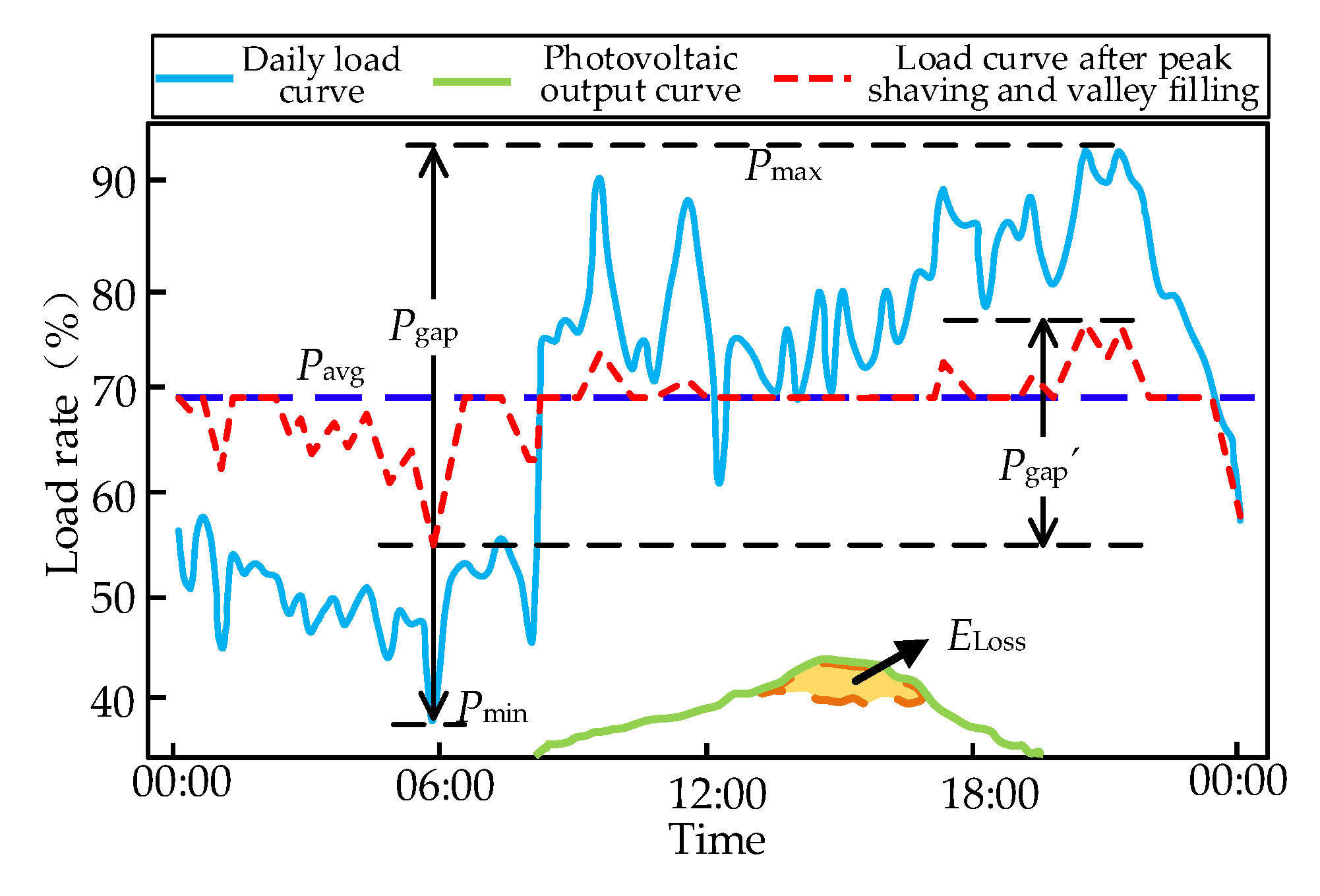
Figure 2.
Beluga whale behavioral.
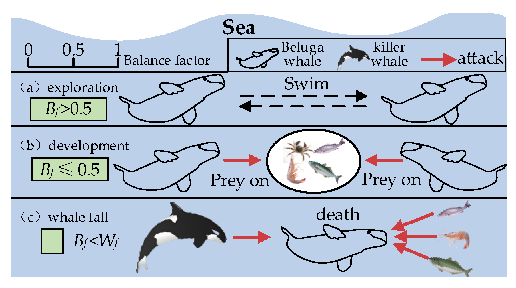
Figure 3.
Flowchart of TWBWO algorithm solving DESS capacity optimization problem.
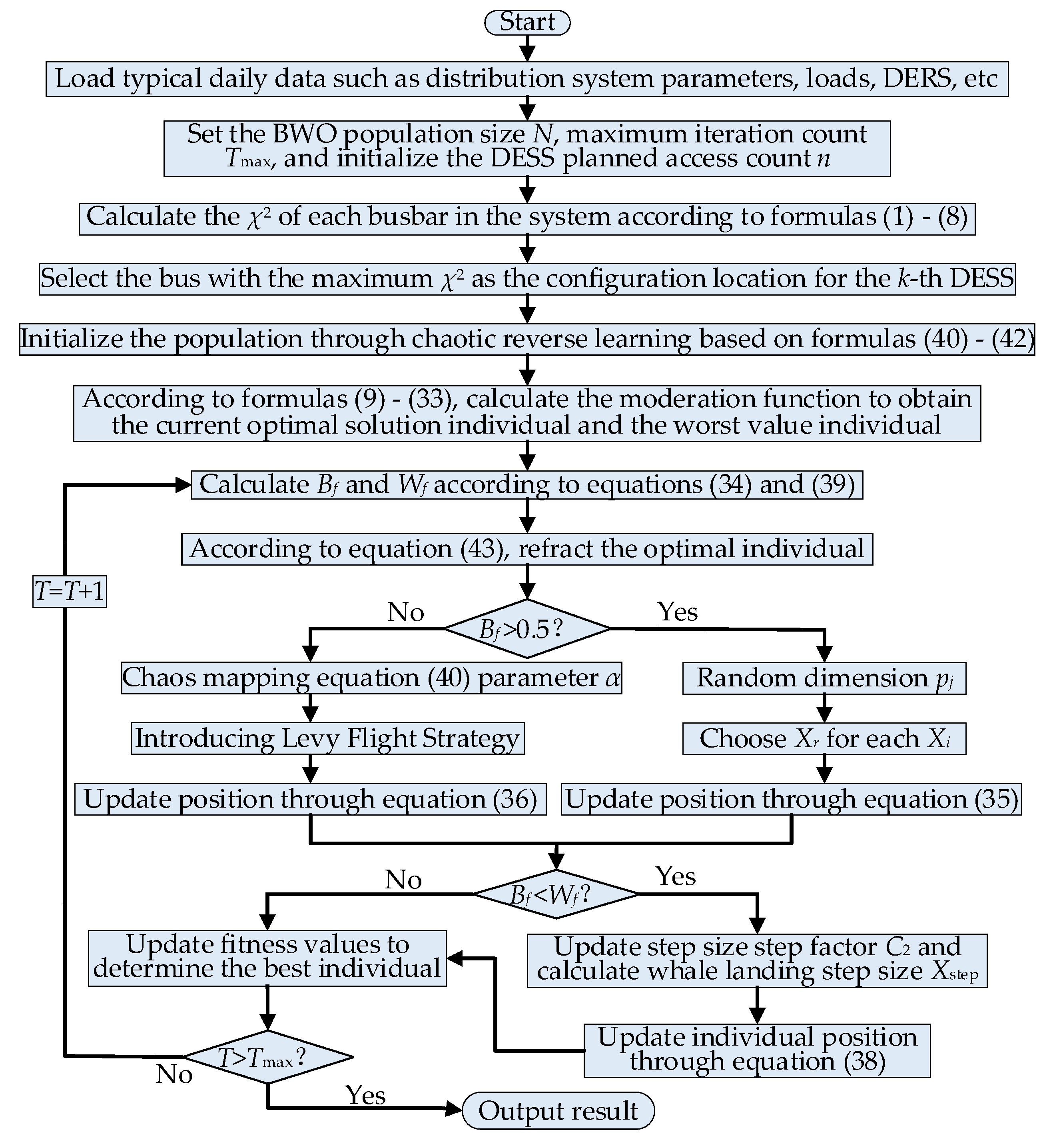
Figure 4.
Modified IEEE-33 node distribution network system.
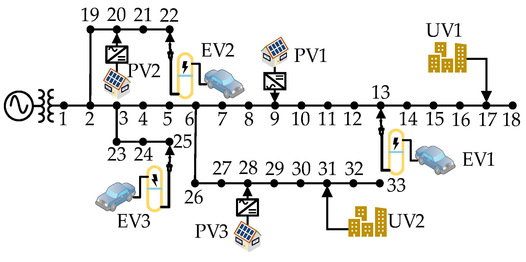
Figure 5.
System operating parameters: (a) Daily load curve and PV output prediction curve;(b) Daily load curve of electric vehicle charging piles and urban villages.
Figure 5.
System operating parameters: (a) Daily load curve and PV output prediction curve;(b) Daily load curve of electric vehicle charging piles and urban villages.
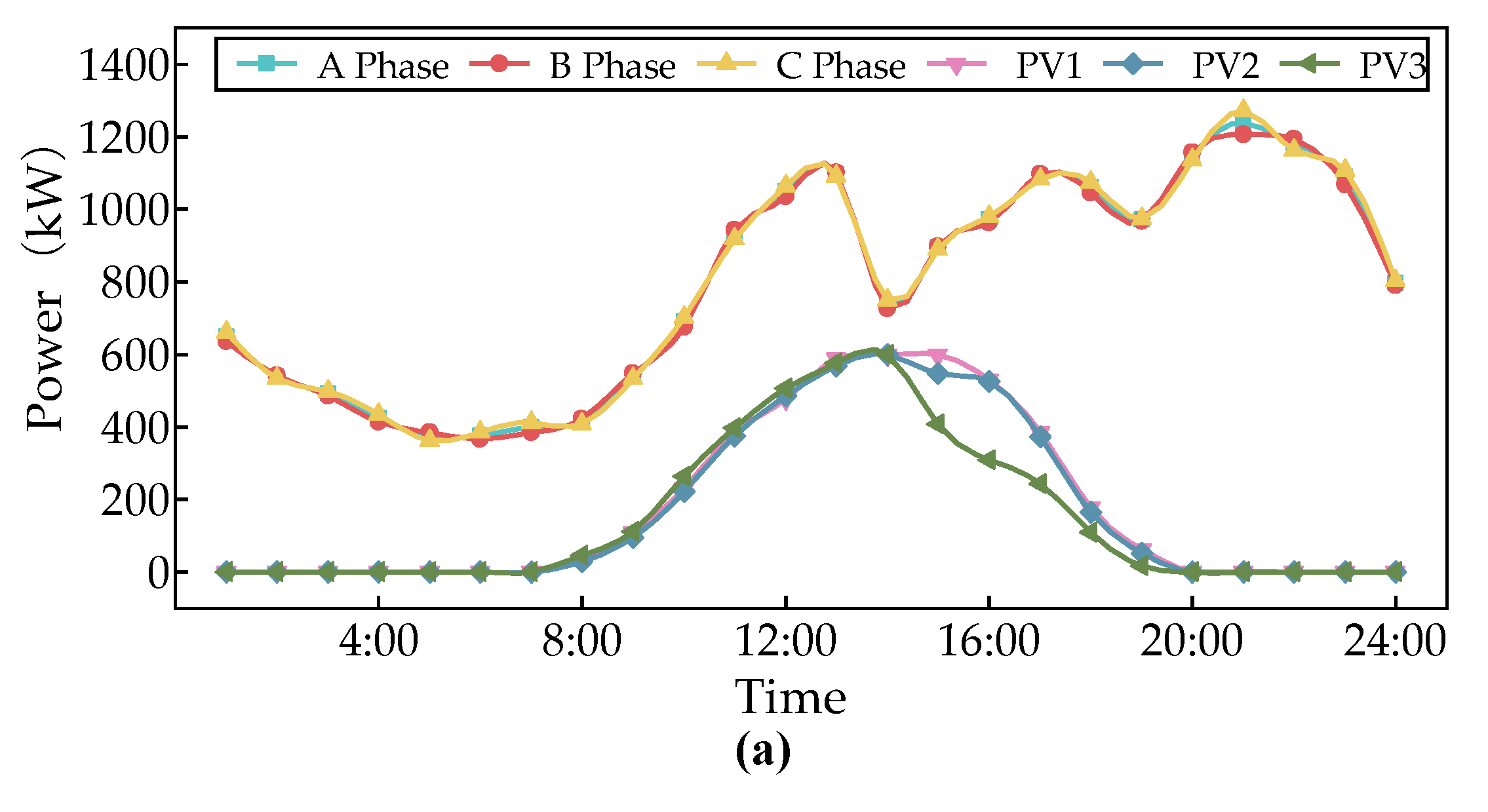

Figure 6.
Comparative chart of comprehensive voltage sensitivity variance: (a)-(c) values of phases A, B, and C in different cases.
Figure 6.
Comparative chart of comprehensive voltage sensitivity variance: (a)-(c) values of phases A, B, and C in different cases.
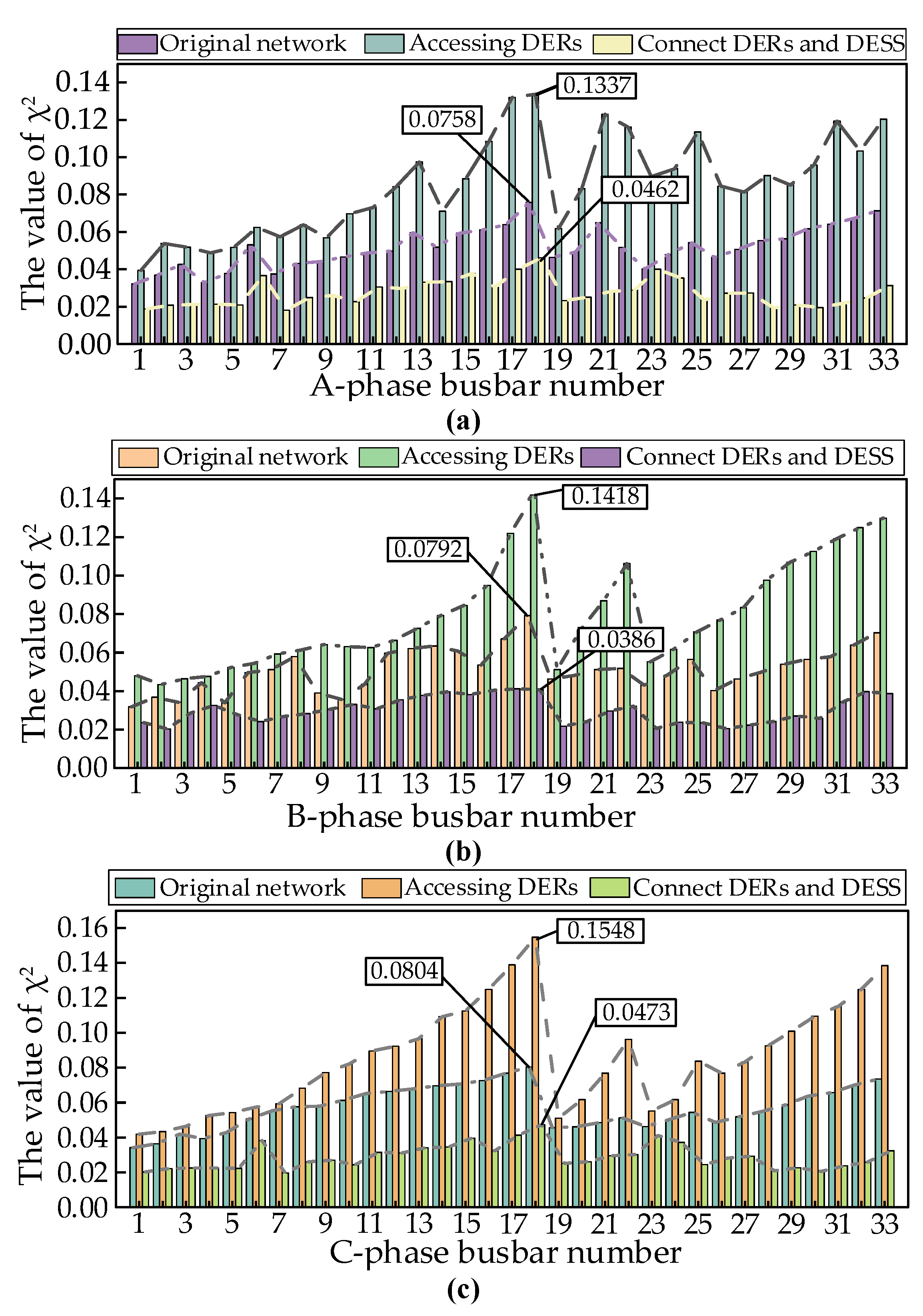
Figure 7.
Distribution of pareto solutions for different algorithms: (a) BWO algorithm; (b) TWBWO algorithm.
Figure 7.
Distribution of pareto solutions for different algorithms: (a) BWO algorithm; (b) TWBWO algorithm.
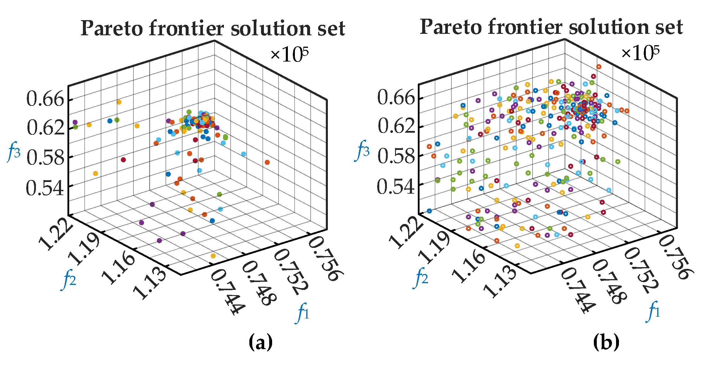
Figure 8.
Convergence curves of two algorithms.
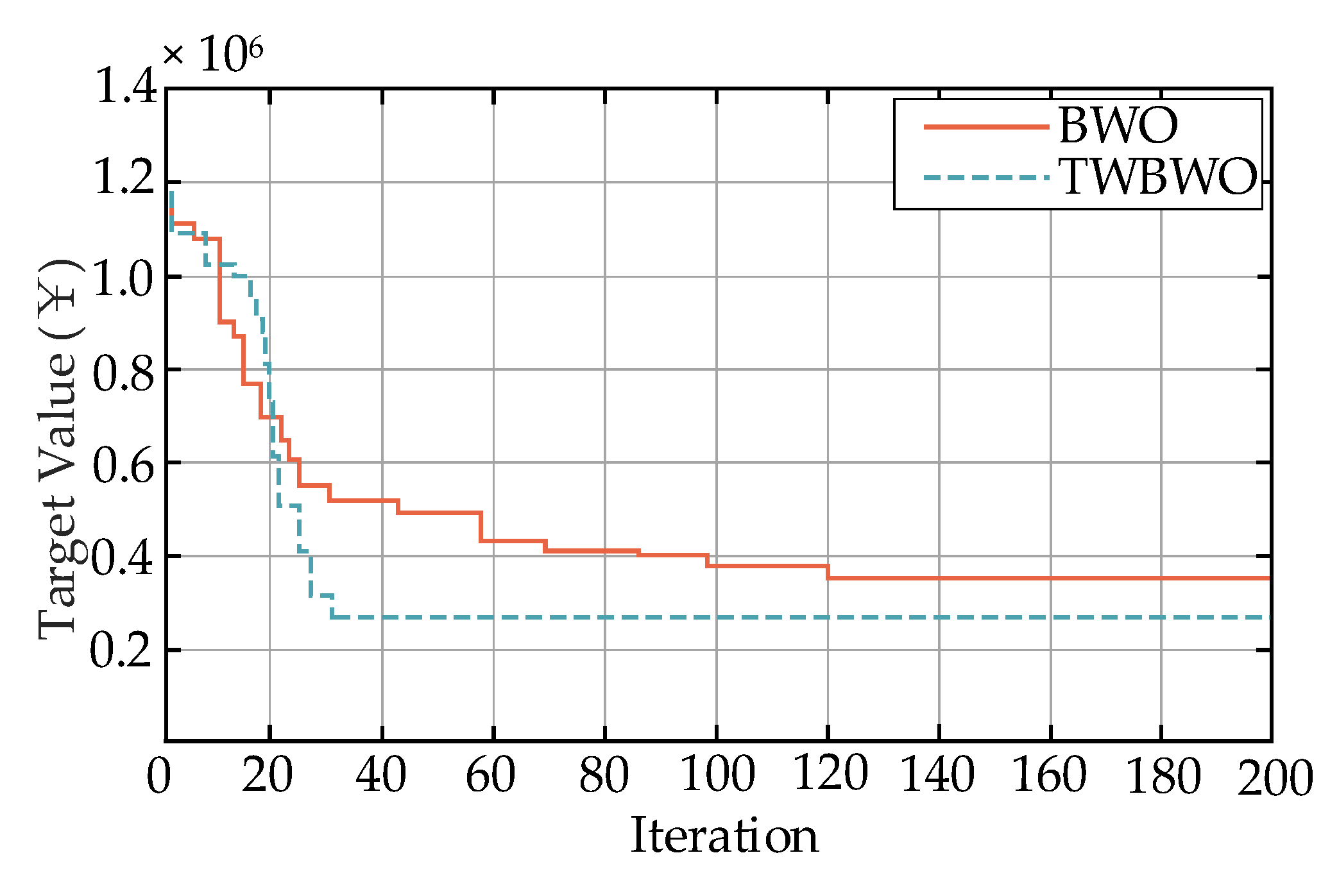
Figure 9.
System daily load curve with different distributed energy resources.
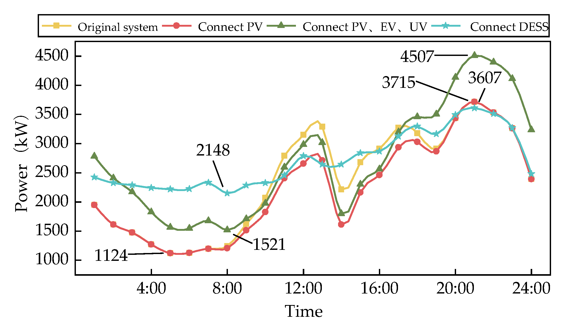
Figure 10.
Charge and discharge curves of 3 sets of DESS.
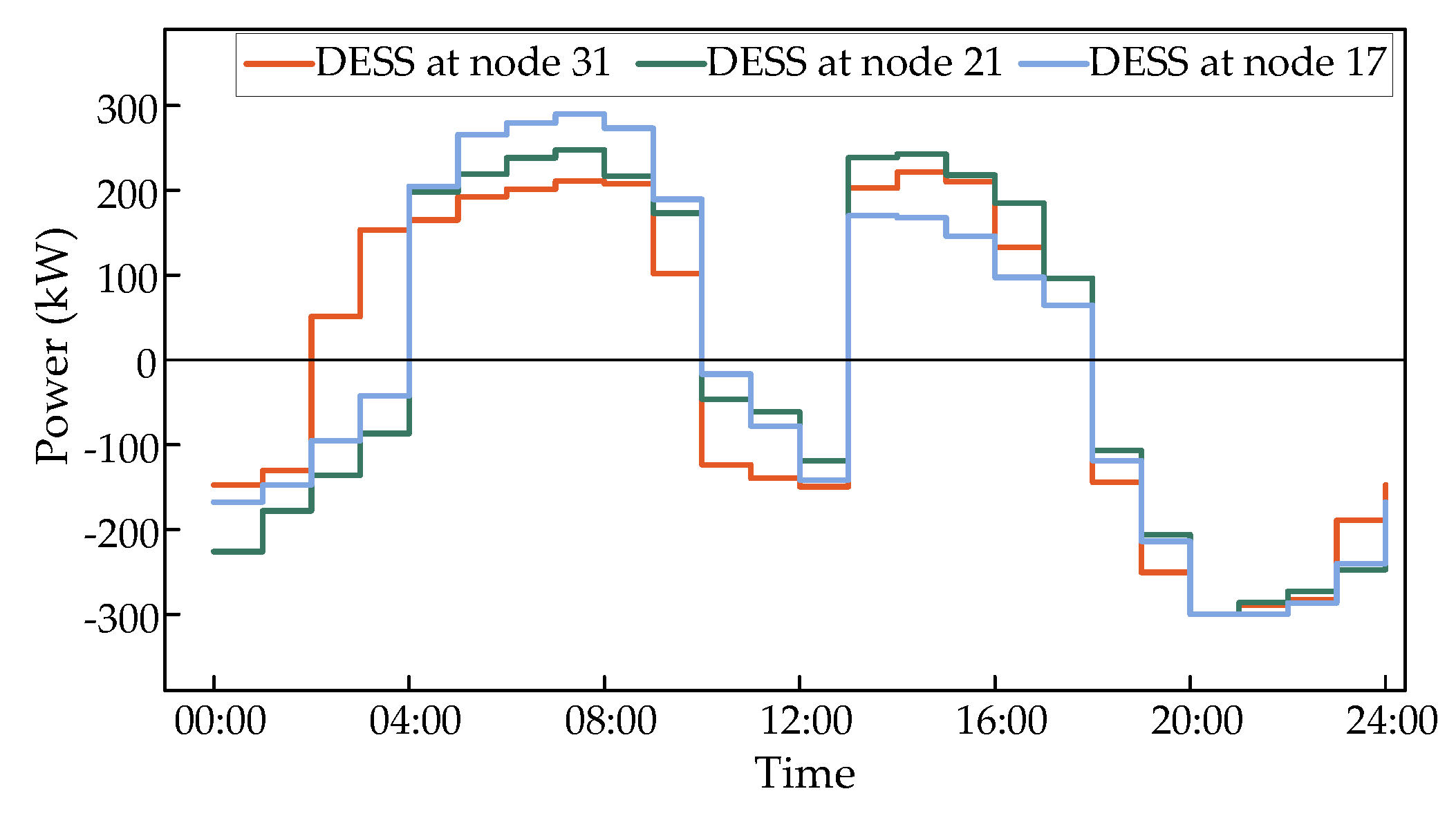
Figure 11.
Topological structure of the actual distribution network system with 199 nodes.
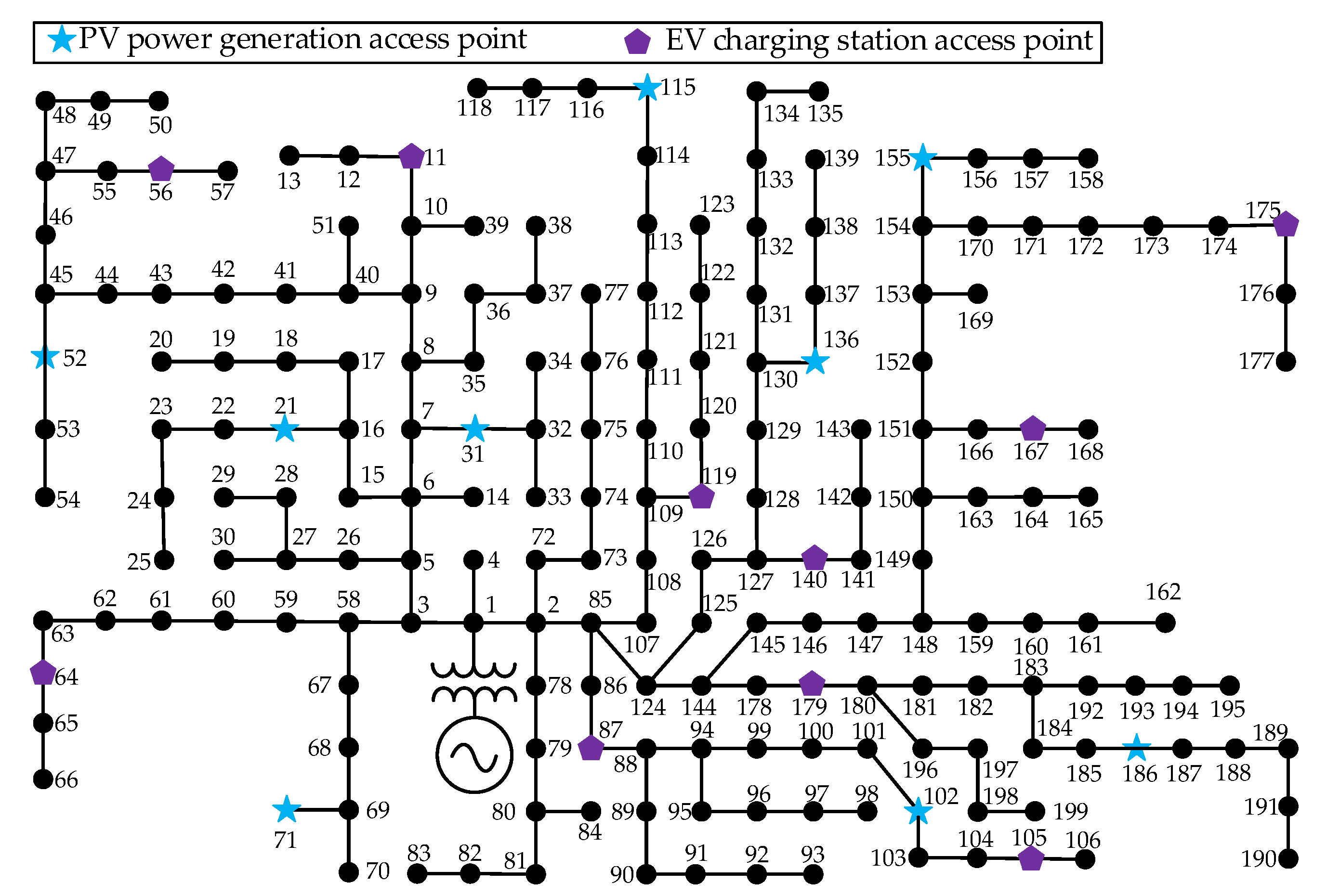
Figure 12.
Heat map of the CPFSV value of 199 nodes over time:(a)-(c)corresponding to working conditions 1, 2, and 3.
Figure 12.
Heat map of the CPFSV value of 199 nodes over time:(a)-(c)corresponding to working conditions 1, 2, and 3.
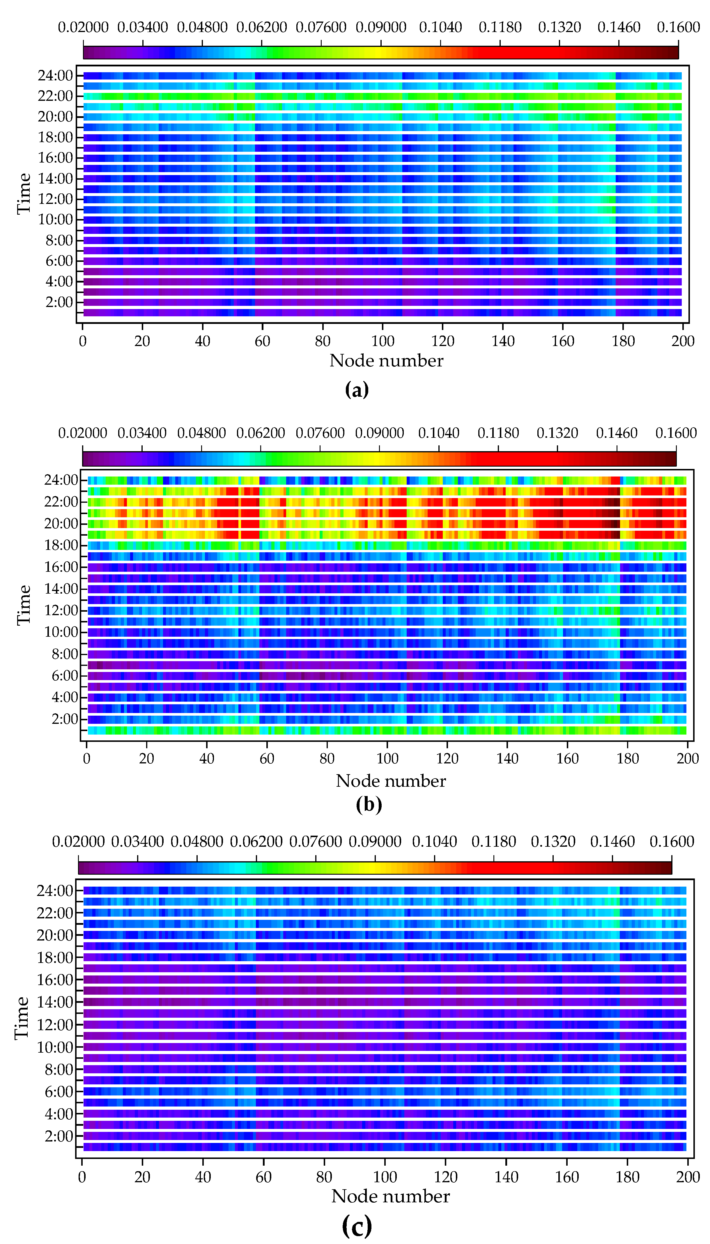
Figure 13.
Load curves under three operating conditions.
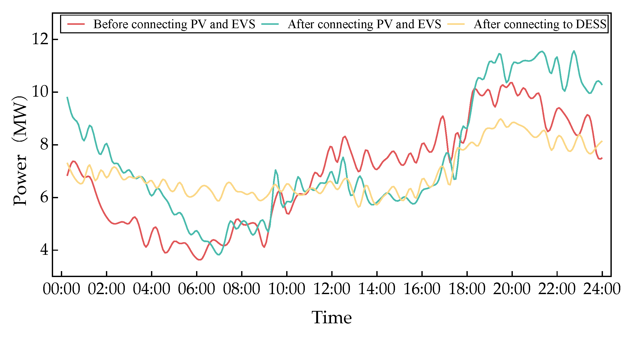
Figure 14.
Contour map of voltage per unit value at each node under two operating conditions: (a)-(b) Corresponding to operating conditions 2 and 3.
Figure 14.
Contour map of voltage per unit value at each node under two operating conditions: (a)-(b) Corresponding to operating conditions 2 and 3.
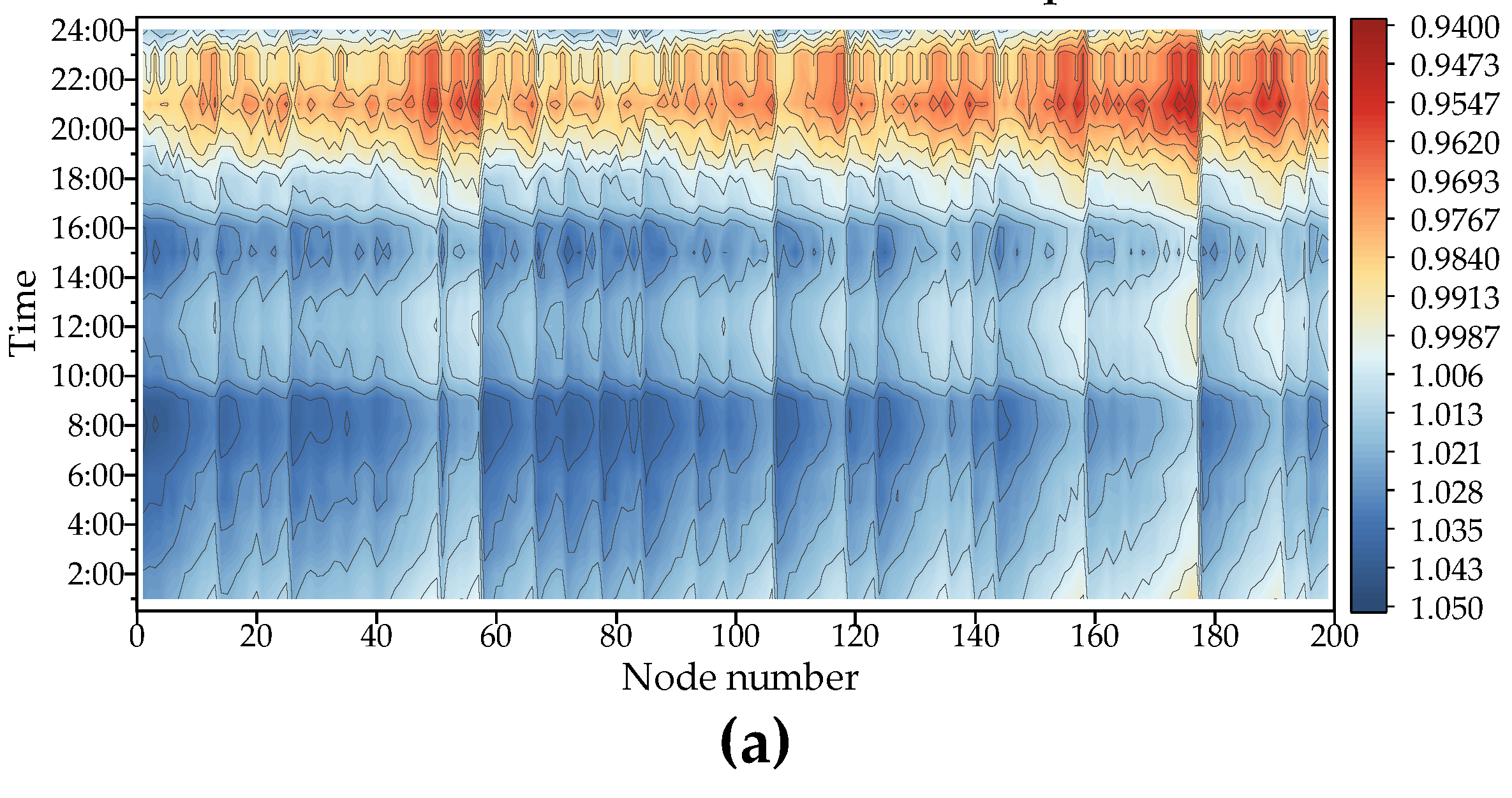
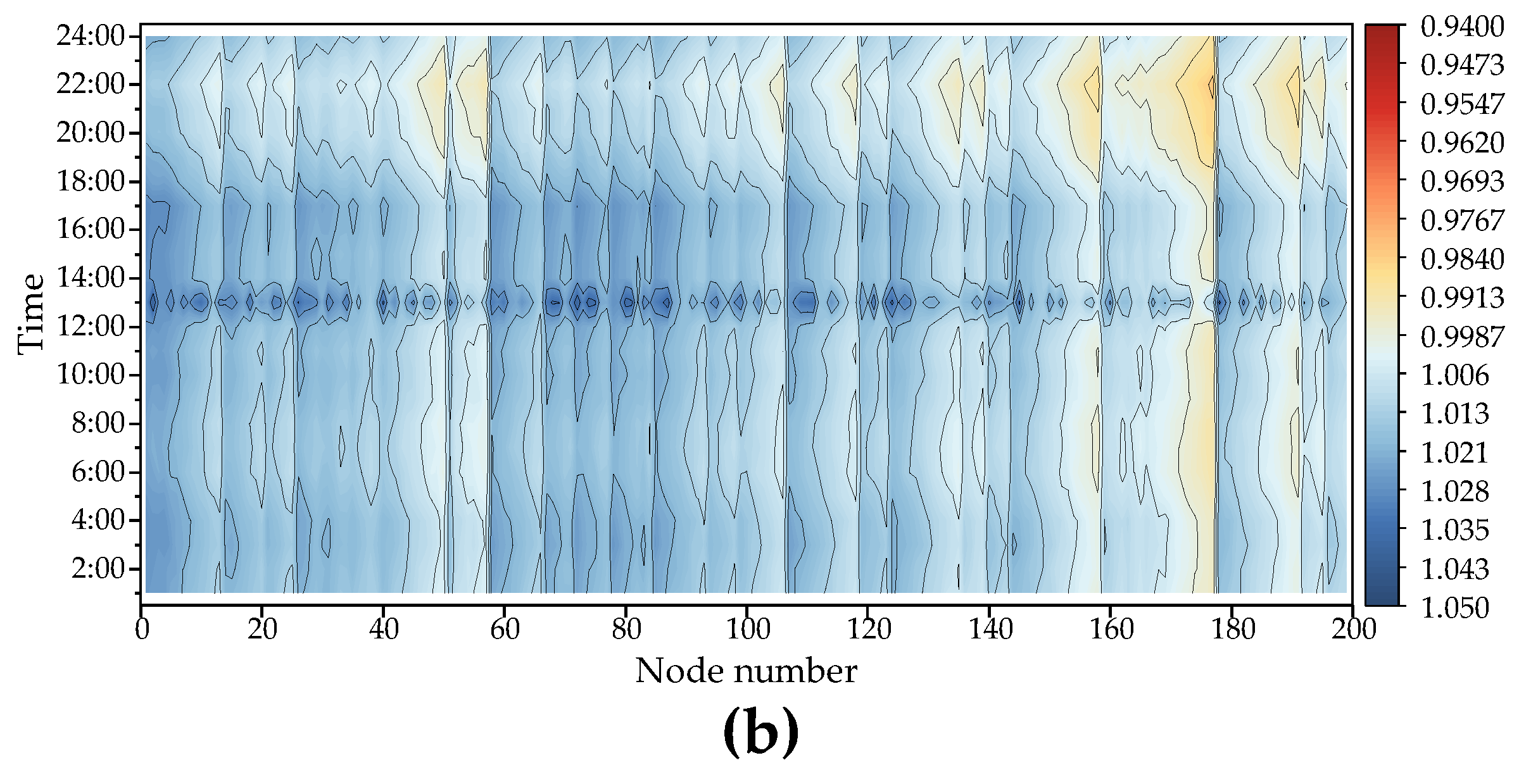
Table 1.
Simulation parameters and variable settings.
| Parameter | Value | Parameter | Value |
| αj(¥/kWh) | 438 | prch(¥/kWh) | 0.31 |
| βj(¥/kW) | 657 | prdis(¥/kWh) | 0.62 |
| Cm(¥/kW)/kWh) | 1500 | Smin(%) | 10 |
| Cep(¥/kWh) | 0.51 | Smax(%) | 90 |
| ηnDESS(%) | 1.7% | εmax(%) | 3 |
| ηoeDESS(%) | 98.6% | Umin(p.u) | 0.95 |
| Pmax(kW) | 300 | Umax(p.u) | 1.05 |
| Emax(kWh) | 1500 | r(%) | 19.4 |
| y(year) | 10 | Tmax(Tims) | 200 |
| ηc(%) | 0.95 | Population size n | 30 |
| ηd(%) | 0.95 | spatial dimension D | 100 |
Table 3.
Proportion of various costs in target values under different cases.
| Case | F/¥ | f1/¥(%) | f2/¥(%) | f3/¥(%) |
| Case 1 | 686472.83 | 394035.40(57.4%) | 0 | 292434.43(42.6%) |
| Case 2 | 1676429.73 | 937124.22(55.9%) | 0 | 739305.51(44.1%) |
| Case 3 | 2374831.42 | 688701.11(29%) | 517713.25(21.8) | 1168417.06(49.2%) |
| Case 4 | 3286697.74 | 1018876.30(31%) | 893981.79(27.2%) | 1373839.66(41.8%) |
| Case 5 | 2411175.19 | 612438.50(25.4%) | 713707.86(29.6%) | 1085028.84(45%) |
Table 4.
Composition of energy storage costs under different cases.
| Case | Cost(¥) | ||||
| CPA | COM | CLOSS | CIN | CTOTAL | |
| Case 3 | -64817.2 | 57114.7 | 77146.2 | 94649.2 | 164092.9 |
| Case 4 | -66743.9 | 67362.4 | 83664.9 | 112341.6 | 19662.5 |
| Case 5 | -75034.9 | 53334.2 | 42664.8 | 113241.8 | 134205.9 |
Table 5.
optimal selection of pareto solution set based on TOPSIS method.
| Result | ||||
| Group | f1(¥) | f2(¥) | f3(¥) | F(¥) |
| A | 612310.78 | 713580.31 | 1085284.1 | 2411175.19 |
| B | 614377.86 | 697768.49 | 1109767.13 | 2421913.48 |
| C | 663778.52 | 699674.61 | 1065221.94 | 2428675.07 |
| D | 648862.39 | 685117.65 | 1091963.47 | 2425943.51 |
| E | 638419.97 | 691064.37 | 1088436.59 | 2417920.93 |
Table 6.
Results of DESS access location and capacity allocation.
| Location | 21 | 50 | 118 | 64 | 134 | 158 | 176 | 190 | 105 |
| 0.115 | 0.138 | 0.133 | 0.118 | 0.126 | 0.151 | 0.159 | 0.147 | 0.127 | |
| EB(MWh) | 1.09 | 1.22 | 1.41 | 1.15 | 1.31 | 1.45 | 1.47 | 1.38 | 1.34 |
| PB(MW) | 0.3 | 0.3 | 0.3 | 0.3 | 0.3 | 0.3 | 0.3 | 0.3 | 0.3 |
Table 7.
Some relevant index values of the system under three operating conditions.
| Operating condition | Index | ||||
| PLOSS(kW.h.d-1) | Pgap(MW) | Umin(pu) | (%) | ||
| 1 | 0.082 | 2176.534 | 6.678 | 0.973 | 2.73% |
| 2 | 0.159 | 3246.137 | 7.698 | 0.948 | 3.69% |
| 3 | 0.071 | 849.283 | 3.257 | 0.985 | 2.18% |
Disclaimer/Publisher’s Note: The statements, opinions and data contained in all publications are solely those of the individual author(s) and contributor(s) and not of MDPI and/or the editor(s). MDPI and/or the editor(s) disclaim responsibility for any injury to people or property resulting from any ideas, methods, instructions or products referred to in the content. |
© 2024 by the authors. Licensee MDPI, Basel, Switzerland. This article is an open access article distributed under the terms and conditions of the Creative Commons Attribution (CC BY) license (http://creativecommons.org/licenses/by/4.0/).
Copyright: This open access article is published under a Creative Commons CC BY 4.0 license, which permit the free download, distribution, and reuse, provided that the author and preprint are cited in any reuse.


