Submitted:
26 September 2025
Posted:
29 September 2025
You are already at the latest version
Abstract
Energy efficiency performance (EEP) in power supply continuously changes depending on the load demand type and operation period. Integrating electric vehicles and battery energy storage (BES) has made it imperative. Therefore, in practice, it might be quite difficult for distribution system operators to concurrently meet the load demands of as many customers as possible at peak loading conditions. In the literature, distributed generation integration for loss minimization is a predominant approach, whereas BES can work as a source or load that can directly or indirectly affect the EEP. This work uses a heuristic technique to create multiple probabilistic loading patterns for EEP of small, medium and extra-large radial networks. The performance indicators such as node voltage profile, loadability, reliability, power losses, and computational efficacy are used. The multi-objective problem is solved using a harmony search algorithm (HSA). For robustness, the performance of the proposed approach is compared with the existing approach available in the literature. Moreover, the EEP is evaluated for 33-, 69-, 85-, 119-, 137- and 417-node radial networks while configuration management with enhanced EEP in the interest of utilities and customers with BES as a load and source exclusively.
Keywords:
energy efficiency performance
; probabilistic loading patterns
; coordinated configuration
; radial distribution networks
; performance indices
; battery energy storage
1. Introduction
Usually, the significant aspects of power system operational performance are energy efficiency and stability under steady state and abnormal state, respectively. However, with growing demand and deregulation, the steady-state duration is much more significant, making the energy efficiency performance (EEP) for coordinated planning and operation imperative. Also, integrating electric vehicles and other energy storage systems has created a new challenge in optimizing energy efficiency. If electric vehicles are charged simultaneously on a large scale, it may cause a peak load increase. Therefore, researchers are more focused on dealing with this new challenge, and several studies have yielded that the operation of distribution systems with mere loss minimization occasionally benefits utilities and customers. This is because the loads, over a given duration, are highly non-uniformly distributed and voltage-dependent. Further, it may impact voltage profile and angle, loadability, reliability, power losses, and the computational efficacy of load flow solution differently. Therefore, load flow studies are required to identify the loading patterns and their voltage dependency to comment upon the EEP of RDNs.
Identification of loading patterns is difficult due to the power system’s changeability, intricacy, and unpredictability. The collective utilization of electricity by various devices constitutes the electrical load of the power system. These devices are commonly interconnected with the distribution network. The existing literature has indicated that the fluctuations in the electrical load play a significant role in determining the stability of the power system [1]. Ihara et al. [2] evaluated the residential load characteristics of the Kansai Electric Power Company’s power system and observed that load modelling helps the power network minimize overall energy usage and improve energy efficiency.
In load flow investigations, there are numerous arteries to model sources and loads. Load types describe the operational parameters of particular loads and are characterized accordingly. Also, different load classes, namely, residential, commercial and industrial loads, show their dependability on voltage and combining load classes with various properties defines practical loads [3]. The existing literature presents insights into load characteristics using static load models for load flow solutions and stability. Through the use of these load models, active and reactive load demands and loadability limits have been emphasized while considering the voltage-dependent characteristics [4]. However, Najafabadi and Alouani [5] address the measurement-based composite load model and propose a real-time framework for evaluating the load model parameters by adopting the approach of multiple model estimation. Chakraborty and Bohre [6] formulated the relation between power and voltage at load busses in the power system. Here, it can be observed that loading patterns are a combined representation of the electricity consumed by all the components in power delivery.
Conversely, Ali et al. [7] described a load flow solution that used a modified branch and bus ordering-based forward-backwards approach to illustrate the consequences of non-linear load models. However, Paul and Paddy [8] implemented a load-shedding and voltage-reduction approach to improve the distribution system’s energy performance. Here, it can be noticed that the load demand has forcefully reduced, and hence, some customers and or particular loads have been isolated from the grid supply. Saini and Gidwani [9] optimized the ideal node for battery placement in the distribution system to minimize daily energy losses, control reverse power flow in the distribution system without going over operational bounds, manage PV penetration, and enhance the voltage profile. Similarly, Jin et al. [10] have proposed DG integration to reduce power loss and improve voltage profile while considering residential, commercial and industrial load models. Here, the energy performance of the distribution system is also evaluated using limited load models, whereas there may be several ways to model these loads, and EEP can be evaluated by considering several other parameters.
Distribution network efficiency can be predicted using other characteristics, such as loadability, reliability, and line drops, as well as voltage profile and losses. Kumar et al. [11] have studied the effect of different load models on loadability with demand-side management techniques. Conversely, Bosisio et al. [21] have developed an approach for energy delivery in a distribution system following a permanent outage while taking resilience and reliability into account. Also, Ali et al. [13] presented the DG placement with reliability as a major concern in their objective function. Gupta et al. [14] encompass the role of reliability in distribution systems during reconfiguration. Also, Noori et al. [15] presented optimal static capacitor placement for improvement in reliability along with minimization in loss reduction and voltage profile. Here, the authors have formulated optimization problems with multi-objective functions. However, no emphasis has been laid on the loadability margin in these works.
Similarly, Kumar et al. [16] presented a multi-objective approach using heuristic and meta-heuristics for energy efficiency in RDN considering loadability margins. Here, loadability is evaluated with a fixed sending end voltage for each node, and reliability is ignored. However, Ali et al. [17] discussed the reliability and loadability margins in their objective formulation, but both objectives have been formulated in such a way that reliability is calculated for the overall system and loadability is obtained by fixing the sending end voltage for each node. Mendoza et al. [18] and Wang et al. [19] performed network reconfiguration with constant power load for loss minimization as a major component in their objective function formulations. However, in [18], the reliability issue has also been addressed, but only for constant power load. Conversely, in [20], a multi-objective approach is considered for optimization with time intervals, and network reconfiguration is performed to minimize loss. The network reconfiguration appears with static load models in [21] and [22] with different objectives. However, Shirdar et al. [23] proposed a multi-objective approach in the presence of an energy storage system for improvement in EEP. Kumar et al. [24] evaluated the EEP of distribution systems under varying loading patterns, whereas static and dynamic load models were considered in [25] for different objectives. Similarly, optimal DG allocation is done in the distribution system under different load models [26]. But, in [27], the EEP of distribution is evaluated and improved by considering the several external energy sources using a multi-objective function. Further, reconfiguration of RDNs is performed in [28] and [29], where computational time is emphasized while minimizing the power loss in the new topology.
The above literature review reveals that the EEP of an RDN depends upon the load flow solution techniques, load patterns in a given network configuration and integration of external energy boosters. Here, it can also be observed that, in the existing literature, the EEP of the distribution system is predominantly evaluated with loss minimization and voltage profile improvement. Generally, constant power load is modeled, and the loadability and reliability margin is evaluated for the overall network, whereas these parameters need to be evaluated at each node. In addition, in recent years, the integration of BES, particularly electric vehicles, can significantly influence the EEP of the distribution system. In practice, BES can work as a load while charging, and as a source during discharging and therefore, it will modify the practical load patterns, which are unpredictable in advance. Considering this fact, this work presented the ten different voltage-dependent and independent load combinations for comprehensive evaluation of the EEP of the distribution system. EEP under different probabilistic loading patterns is evaluated in different configurations available in the literature for different objectives. Moreover, the proposed work presented the computation performance of different load flow solutions, energy efficiency performance under various probability loading patterns and the effect of integrating BES as load or source, exclusively in 33-, 137- and 417-node RDNs.
2. Solution Techniques and Radiality
The convergence characteristics of the radial distribution optimization problems depend upon the types of load flow techniques and the method to maintain the network radiality. The load flow solution of RDN uses the forward-backwards sweep method because of its computation efficacy and robustness. However, the iteration in forward-backwards sweep methods can be performed in three ways: voltage iteration, current iteration, and load demand iteration. The number of iterations for convergence of solutions in these techniques varies differently.
2.1. Iterative Methods
The computational performance of iterative methods depends on the number of radial paths formed, the initial guess for node voltage profile and line power losses. Therefore, voltage, branch current, and demand-based iterative methods are explored as under,
Step 1: Assume a flat voltage profile, (Vi =1.0), and set initial power loss & line current as zero.
Step 2: Identify the loading pattern i.e. LM-1, LM-2 ……… and LM-10.
Step 3: Set convergence criterion as e=0.0001 and iteration count k= 0.
Step 4: Calculate power demand at each node as the sum of self-node power and demand of downstream nodes and line losses.
Step 5: Compute node current, loadability, reliability, and new node voltages.
Step 6: Compare all old and new values of the following:
- i.
- For voltage iteration: Node voltage and check if max|Vk-Vk+1| is less than ‘e’; if yes, go to the next step. Else, repeat steps 2 to 5.
- ii.
- ii. For Current iteration: Node current and check if max|Ik-Ik+1| is less than ‘e’; if yes, go to the next step. Else, repeat steps 2 to 5.
- iii.
- iii. For demand iteration: Node demand and check if max|Pk-Pk+1| is less than ‘e’; if yes, go to next step. Else, repeat steps 2 to 5.
Step 7: Print iteration counts, convergence time and load flow results.
As discussed above, the iterative methods can be evaluated based on their computation time (CT) and load flow results. The number of counts and CT of these methods is shown in Table 1. Here, voltage iterative method is further explored since it has low CT and less iteration counts.
2.2. Network Radiality
Radiality can be described using the number of branch and their sending and receiving end nodes. To identify the receiving end node of a branch it has become imperative to determine the number of radial paths in a given network. Therefore, to state the topology of the radial network having ‘n’ number of nodes, the following conditions are to be satisfied:
Condition 1: A network is said to be radial if a branch has only one receiving end node, whereas a node may be a sending end node for multiple branches.
Condition 2: Every node, except the source node, is a receiving end node once in a while in network configuration management.
The total branches of a network can be divided into connected branch (Ωcb) and tie-line (ΩTb). Let, Ωb– be the set of branches, Ωs– be the set of sending end nodes, Ωr– be the set of receiving end nodes of a radial network. Therefore,
A sample network, as shown in Figure 1, is considered to illustrate network radiality. Here, there are eight nodes and nine branches. The branches 8 and 9 are tie lines and the connected branches are 1–7, and the set of their sending and receiving end nodes are,
The branches which create a loop in the network are [2 3 4 5 8] and [3 4 5 9]. Branches 8 and 9 have their receiving ends repeated as in . This will violate radiality condition-1, and therefore, one branch from each loop is required to be replaced with a tie-line. However, here, it can be noticed that if two such branches are 3 and 4, then node number 4 will be an isolated node. This means node 4 will not be a receiving end node for any branch in the given network topology, and hence, it violates the radiality condition 2. In the proposed work, the radiality is addressed by identifying the radial paths before performing the load flow solution. This will reduce computational effort and help the algorithm to converge fast. The identification of radial paths is illustrated in three cases;
Case-1: If branches 8 and 9 are the tie-lines, then there will be a single radial path having sending end node (), receiving end node () and branches (), such as,
Case-2: If branches 2 and 6 are the tie-lines, then there will be a single radial path having nodes and branches, such as,
Case-3: If branches 4 and 6 are the tie-lines, then there will be three radial paths having nodes and branches, such as,
In addition to the above, the branches 3, 4 and 5 are common in loop-1 and 2. Replacing any such branches with tie-lines violates radiality condition-1; therefore, these branches cannot be chosen simultaneously in both loops while reconfiguring the network topology. This will further reduce the possibility of violation of radiality and, hence, the computational time.
3. Probabilistic Loading Patterns
Practical loads in the distribution system vary with variations in the system voltage profile. Therefore, loads can be classified into two categories: fixed pattern loads and variable pattern loads.
- Fixed pattern loads: The fixed pattern loads can be further classified as load types and load classes. Table 2 shows the different load types and class,
- Variable pattern loads: The variable pattern loads can also be classified into two parts, i.e. composite load pattern and grouped load pattern.
- i.
- Composite load: These loads can be modelled using either load types or load classes at each node. However, the composition of a particular type of load may be different and or obtained using the random distribution function
The above equation represents the modelling of LM-7 and LM-8, which is a composite effect of LM-1, LM-2 and LM-3 for LM-7, whereas LM-4, LM-5 and LM-6 for LM-8. Here, for the active component of load demand, the fractions p1, p2 and p3 represent the contribution of load type at the respective node and , , and are the voltage exponents for LM-1, LM-2 and LM-3 respectively. The load fractions are chosen such that,
Similarly, for a reactive component of load demand, fractions q1, q2 and q3 and exponents , , and are used for the modeling of LM-7. Conversely, LM-4, LM-5 and LM-6 are used for LM-8 with their fractions and exponents, respectively.
- ii.
- Grouped load: These loads can be modelled using either load types or load classes at respective nodes. However, the composition of a particular type of load may be different and or obtained using a random distribution function. For LM-9, the number of nodes is selected at random, having only LM-1, LM-2 and LM-3, whereas, LM-4, LM-5 and LM-6 are used for LM-10, and the nodes are selected randomly in this case too.
However, practical loads are voltage-dependent and vary differently depending on the time of operation and type of the loads. All possible combinations of the existing load models must be modelled to evaluate the energy efficiency of distribution systems comprehensively. Therefore, in the proposed work, ten different load models (i.e., from LM-1 to LM-10) are formulated to evaluate the EEP of the distribution systems.
3.1. Performance Metrics
The EEP of the distribution system includes several parameters such as load demand profile, voltage profile, line losses, line voltage drops, loadability and reliability at the respective node and for the overall network. However, EEP can also be influenced by the integration of external energy sources like distributed energy resources, energy storage systems, shunt capacitors, etc. The following are the performance matrices,
3.1.1. Load Demand Profile
In an RDN, the load demand at respective nodes is the sum of the loads of the downstream nodes, line losses, and demand for the node itself. Therefore, at a respective node, the active and reactive components of power are calculated as follows,
In (9) and (10), the first component is the load demand of the node itself, the second component represents the sum of load demand beyond the ith node, and the third component represents the line losses beyond the ith node in a given network configuration.
3.1.2. Node Voltage Profile
Figure 1 represents the equivalent radial network where Vi and Vj are the sending-end and receiving-end voltages. ri and xi are the line resistance and reactance. PTi and QTi are the resultant load demands at receiving-end node.
Figure 2.
A sample equivalent RDN.
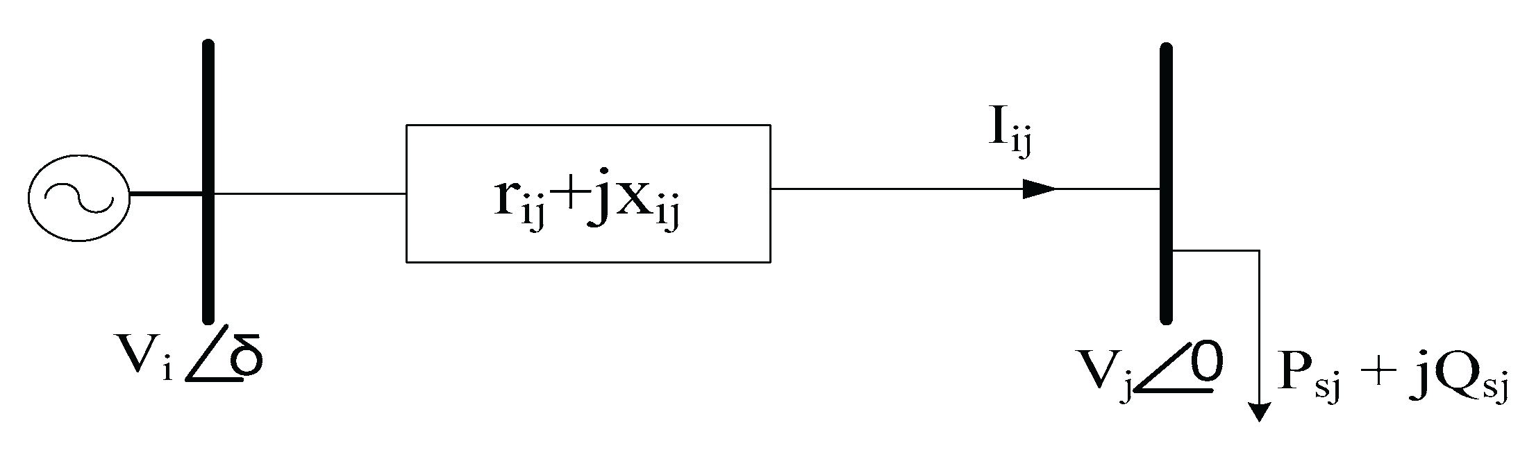
From the equivalent network the following relations can be derived,
On rearranging (14) and substituting the value of current and angles in terms of active and reactive components power, the receiving end voltage can be obtained using (15),
3.1.3. Line Loss
Line loss in an RDN depends upon the number of downstream nodes and their load profile. Therefore, the active and reactive line loss can be calculated using (16) and (17),
3.1.4. Loadability
Loadability is the capacity of the power feeder to withstand the maximum load at a given voltage and line parameters. It can be evaluated in two ways: (a) when node voltage at each node is fixed and (b) when only substation voltage is fixed. In the first case, the loadability indicates the capacity of a line segment only, whereas, in the second case, the loadability of the power feeder starting from the substation to the load point is estimated. Therefore, if a network is stable according to the first loadability criterion, it may fail in the second criterion. In this work, these two criteria are described as follows,
Criterion-1: In this criterion, the sending end node voltage at each node is considered fixed, and in order to find the loadability at receiving end nodes, the component of equation (15) should be greater than or equal to zero. Therefore,
To define the maximum load that can be connected at the respective nodes, the existing load is replaced by and (19) is further modified as a quadratic form of ‘’ and on solving, it yields.
Criterion-2: This criterion considers the effect of voltage drops from the source node to the candidate node. Therefore, eq. (19) is modified as (20),
In (20), the ,, and are voltage at source node, Thevenin’s equivalent resistance and reactance between source node and candidate node, respectively. Here, the Thevenin’s equivalent impedance is calculated as,
In (21), ‘BRP’ is the number of branches in a radial path starting from source node. Ik is current at the respective node where the equivalent impedance is to be calculated. Separating the real and imaginary part of equivalent impedance, the equivalent line resistance and reactance are calculated using (22),
3.1.5. Reliability
Reliability represents the system’s performance and how well it functions when subjected to regular failures over a particular period. The reliability of a network can be evaluated at each node and for the overall network. Generally, in the existing literature, the reliability of the overall network is calculated, whereas, in this work, the performance of the network is evaluated based on both criteria. The mathematical calculations for reliability are described as follows,
Criterion-1: In this criterion, the frequency of interruption (Fsys), duration of interruption (Tsys) and energy not supplied (ENSsys) are evaluated for the whole system in one go, as shown in (23)-(25).
Here, i.e. kVA demand at respective node only. n-1 is the number of nodes except the source node. The relationship between repair time and failure rate is depicted using (26).
The reliability index of the whole system is represented using (27). Here, the weightage of each component is taken uniformly; however, depending upon the operating constraints, their weightage may differ.
Criterion 2: In this criterion, the reliability of a radial path is evaluated differently. Here, the nodes in a radial path, starting from the source node, are listed, and Fj, Tj and ENSj are calculated.
In (28)-(30), ‘NRP’ is the number of nodes in a radial path starting from source node. Also, is the sum of kVA demand at respective nodes due to demand on downstream nodes. Therefore, knowing the values of Fj, Tj and ENSj, the reliability index of the network is calculated using (31).
3.1.7. BES Integration
The battery energy storage (BES) may vary with charging or discharging states. During the charging state, BES work as a load and cause extra loading over the system while discharging; it acts as a source and relieves the burden of the existing system at peak loading conditions. Therefore, modelling BES requires their formulation as a source and load at different instants of time. The modelling of BES during charging/discharging and or as a load/source is described using (32);
When BES works as a source, the SOC is calculated as under,
When BES works as a load, the SOC is calculated as under,
Here, in (33) and (34), the is the state of charge of BES at ith time instant, is the previous state of charge, is the discharge and is the charge capacity at that instant of time. ‘’ and is the charge and discharge efficiency, respectively. ‘’ is the time duration for which BES is allowed to be charge or discharge. The selection of ‘’ depends upon the operating conditions and loading patterns, which is not in the scope of this work. In the proposed work, BES is considered fully charged or discharged when it works as either a source or load to evaluate the EEP of RDNs under varying loading patterns.
4. Problem Formulation and Objective Functions
In the proposed work, the problem is formulated with many objectives and represented as follows,
Here, in (35), ‘’ is the respective index and ‘k’ is the size of the index array. ‘’ is the weighting factor of the respective index and it is taken uniformly for the same weightage of each index. ‘Xp’ is the penalty factor on OF which is the ratio of power loss in the base configuration and resulting network topology. In the proposed work, the various objectives are formulated based on the system voltage profile, line losses, load demand profile, reliability and loadability. The various indices are described as follows,
- (I)
- Node Voltage Index: Voltage at each node varies differently due to variations in loading patterns, and the load patterns are voltage-dependent, which in turn performs poorly at low voltage.
In (36), the NVI varies from ‘0’ to ‘1’. It is minimum when the respective node voltage is equal to the minimum voltage, and it will be maximum when it becomes equal to the maximum voltage. Therefore, the NVI should be maximized to improve the distribution system’s EEP.
- (II)
- Node Demand Index: Load at the respective node is different, and it is the sum of demands of downstream nodes and line loss, which depends upon the network topology and node voltage profile. Therefore, for load balancing at respective nodes, the load balancing profile is indexed as,
In (37), NDI varies from ‘0’ to ‘1’. It is minimum when the respective node demand is equal to the maximum demand, and it will be maximum when it becomes equal to the minimum demand. For energy-efficient operation, the NDI must be maximized.
- (III)
- Node Loadability Index: Load at the respective node defines how much extra load, in terms of the number of customers, can be connected, and therefore, the loadability, i.e. additional load that can be served at a respective node, is indexed as,
In (38), the NLI varies from ‘0’ to ‘1’. It is minimum when respective node loadability is equal to the minimum value, and it will be maximum when it becomes equal to the maximum value of the given network topology. Therefore, the NLI is to be maximized to improve the distribution system’s EEP.
- (IV)
- Node Reliability Index: Reliability at each node depends upon the number and duration of interruptions. As a result, the uneven load demand may cause variation in the reliability of supplying power at a respective node. Therefore, the relative reliability index is formulated as,
In (39), NRI varies from ‘0’ to ‘1’. It is minimum when respective node reliability index is equal to the maximum value, and it will be maximum when it becomes equal to the minimum value of the given network topology. For energy-efficient operation, the NRI must be maximized.
- (V)
- Node Power Loss Index: The power loss beyond a respective node depends upon the network topology and varies differently in different branches. The node after which demand is high will have a high loss and vice versa. Therefore, the node power loss index is formulated as,
In (40), NPI varies from ‘0’ to ‘1’. It is minimum when respective node power loss is equal to the maximum value, and it will be maximum when it becomes equal to the minimum value of the given network topology. For energy-efficient operation, the NPI must be maximized.
The above objective functions are subject to the following operating constraints,
Equations (41)-(43), describes the operating constraints for node voltage, system power loss and, load demand and generation, corresponding to the related objective functions for reliable operation. Violating any one constraint may lead to poor operation of distribution systems. In addition to the above constraints, BES integration needs to be considered as follows,
5. Harmony Search Algorithm
In a radial distribution network, reconfiguration is a discrete problem that has no fixed solution. Therefore, developing a heuristic and/or meta-heuristic approach is required to solve such problems. The proposed work uses the harmony search algorithm (HSA) for configuration management with battery energy storage for different probabilistic loading patterns. Here, the optimization is performed for three cases, namely;
Case-1: With and without BES allocation in the base configuration
Case-2: With and without BES allocation in optimal configuration
Case-3: Reconfiguration and BES allocation in coordination
HSA is a nature-inspired approach in which the optimization function is improvised based on three rules, namely, random search, harmony memory consideration rate and pitch adjustment. Initially, harmony memory (HM) is created randomly with several harmony solution vectors (HSV) where a single solution vector represents the combination of tie-lines and the size and location of BES. The HSA parameters are harmony memory considering rate (HMCR), harmony memory size (HMS), pitch adjustment rate (PAR), bandwidth (BW) and maximum improvisation (MI). A detailed explanation of HSA parameters and their selection is given in [3,21], and [24]; however, the modification in HSA and load flow solution is proposed hereunder;
- A.
- Harmony initialization: HM is a set of solution vectors where each solution vector’s solution is stored in ascending or descending order. In HSA, a single solution vector can be created for tie-lines and BES allocation (size and location).
In HM, the solution vector can be defined in three ways as per the cases of optimization, such as,
Here, for coordination operation, the HSV=, represents the tie-lines and node points for BES allocation simultaneously, for reconfiguration, HSV= represents the tie-lines only whereas, HSV= represents the node points for BES allocation only when their size is fixed.
Therefore, the size of HM can affect the results, and too big or too small HM may result in local optimization as described in [24].
- B.
- Harmony Improvisation: Harmony improvisation involves three steps: random search, HMCR and pitch adjustment.
- Random search: Initially, a solution vector is randomly selected from the global solution space based on random distribution function using rand(). If rand() is greater than (1-HMCR), then is selected from global solution space and the end terminal voltages of the newly selected branch are compared with the existing branch end terminal voltages as,
rand()
ifrand()<PINV
check if Vse,hv < Vse,tie && Vre,hv < Vse,tie
check if Vse,hv < Vre,tie && Vre,hv < Vre,tie
end
In the proposed work, PINV is taken at 0.8, and the effect of PINV over the EEP is evaluated in the later part of the manuscript.
- c.
- Harmony memory considering rate: If rand() is less than HMCR, then a new solution vector, i.e. is selected from HM with no prior conditions.
- c.
- Pitch adjustment rate: If is selected from HM, then a new random distribution function is generated for the pitch adjustment. Based on the PAR, the bandwidth of each pitch-adjusted HSV is modified. However, with an increase in the number of iterations, the probability of PAR increases and BW decreases [3].
- c.
- Harmony update: The solution of the newly generated HSV is evaluated, and based on the objective function improvement, the new solution vector ( is replaced with the old HSV in ascending or descending order. This process will be repeated till maximum improvisation (MI).
In the proposed work, the HMCR, PAR and HMS are taken as 0.85, 0.40 and 10, respectively, for all optimization cases and networks under consideration. Further, the steps involved in load flow solution using HSA for reconfiguration, BES allocation and coordinated operation are described as follows,
Step-1 Read the line and load data and HSA parameters, i.e., HMCR, HMS, PAR, BW, MI and RUNs.
Step-2 Formulation of a global solution for tie lines and BES allocation for EEP evaluation and reconfiguration in the coordination of BES.
Step-3 Identify the network topology’s tie-lines and its initial known parameters. Consider the case of network topology such as,
- a.
- Base configuration (tie-lines are pre-defined) and set Base=1.
- b.
- Specific configuration (tie-lines are pre-defined) and set Specific=1.
- c.
- Network reconfiguration (tie-lines need to be obtained) and set Coordination=1.
Step-4 Create HM and sort the solution in ascending or descending order corresponding to each solution vector.
Step-5 Check for base=1; if yes, set the tie-lines and go to the next step, else go to step-7.
Step-6 Check if BT=1; if yes, go to step-10 and set HSV for BES allocation, else go to step-11.
Step-7 Check for specific=1; if yes, set the tie-lines and go to the next step.
Step-8 Check if BT=1; if yes, go to step-10 and set HSV for BES allocation, else go to step-11.
Figure 3.
Flow chart for the proposed algorithm.
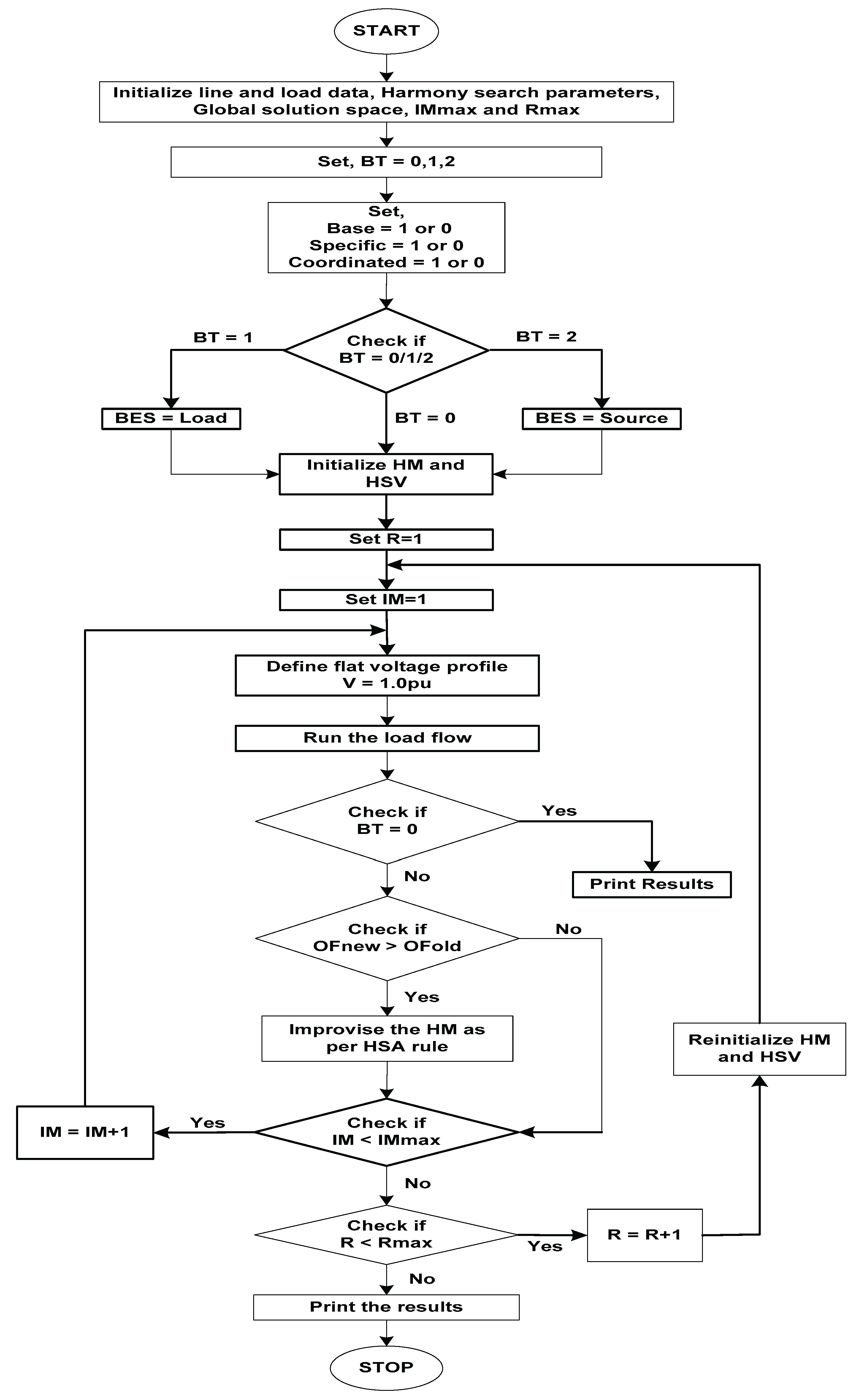
Step-9 Check for coordination=1; if yes, go to the next step and generate the HSV for coordinated configurations, reconfiguration only and BES allocation according to the case of optimization to be performed.
Step-10 Generate a new solution vector as per the HSA rule, i.e. random search, HMCR and pitch adjustment.
Step-11 Set [EN1] as one end and [EN2] as the second end of the branch [BR1] to identify the sending end and receiving end node of a branch.
Step-12 Start from the first branch, consider the first node as the sending end node of this branch and identify the receiving end node by comparing it from [EN1] and [EN2]. Store the information in a new set of end nodes as [SE] and [RE] for the sending end and receiving end of [BR], respectively.
Step-13 Identify the number of junctions at which radial paths bifurcate.
Step-14 Starting from the source node, identify the number of radial paths and the branch and node number in each path. Also, count the number of branches and nodes in these paths.
Step-15 Assume flat voltage profile (i.e.1.0pu) and losses in each branch as zero.
Step-16 Calculate the active and reactive power demand at each node, as described in Section 3.
Step-17 Run the load flow solution described in Section 2.1 and obtain the load flow results.
Step-18 Check if Coordination = 1; if yes, go to the next step, or else print the load flow results.
Step-19 Compare the set objective function with the previous value. If improved, then improvise the HM, as per the HSA rule.
Step-20 Check if IM = IMmax; if yes, go to the next step; otherwise, set IM = IM + 1 and repeat from step-10.
Step-21Check if RUN = RUNmax; if yes, go to the next step; otherwise, set R = R + 1 and repeat from step-9.
Step-22 Print the average computation time of maximum RUNs and the load flow results for each RUN for comparison.
The optimisation above is performed separately for each load model and network for multi-objective function and improvement in an individual index developed for overall EEP of radial distribution networks, i.e. 33-, 69-, 85-, 119-, 137- and 417-nodes.
6. Sample Network and Performance Evaluation
The proposed work considers six different radial networks, varying from small to extra-large, and the optimization problem is formulated in MATLAB 2018b environment. The six networks are 33, 69, 85, 119, 137 and 417-node RDNs. The EEP of these networks is evaluated based on five different indices: voltage profile, demand profile, power loss, loadability, and reliability. The multi-objective function is formulated using (36), as described in section 4. EEP of the networks under consideration have been extensively evaluated individually for the base and reconfigured networks in the presence of BES as a load and source, respectively. In this work, the BES is placed at three locations of size 50, 60 and 70kW, which is considered fixed for EEP evaluation of different RDNs. BES placement is presented using three strategies;
- BES integration in base configuration
- BES integration in optimal configuration
- BES integration in the coordination of configuration management
A 33-node RDN is shown in Figure 4. It comprises 33 nodes, 32 branches, 5 tie-lines, and four radial paths in the base configuration. The first node is the substation at which a voltage of 1.0pu is fixed. The fluctuation of node voltage and active power loss in the 33-node system is shown in Figure 5 and 6 for different LMs. Among all load models, node 18 consistently displays the lowest voltage level, while node 2 consistently reflects the greatest voltage. As the node moves away from the source node or substation, its voltage profile declines, as shown in Figure 5
Conversely, the line power losses are denser in the branches near the substation, and little line losses can be observed in the branches away from the source, as shown in Figure 6. For this network, in the base and optimal configuration is 1.1231 and 1.1087, whereas is 1.0402 and 0.6159, respectively. Here, the RI indicator has improved significantly with as compared to the .
Conversely, the loadability index (LI) is evaluated with two different criteria where: in the first criterion, the LI is calculated by fixing the node voltage at each node and in the second criterion, the substation voltage is taken reference, and equivalent Thevenin’s impedance is calculated up to respective nodes. In criterion-1, the LI is maximum at end nodes, whereas, for criterion-2, the LI is maximum near the source node, as shown in Figure 7 and Figure 8, respectively. Figure 9 shows the reliability index where it can be observed that the RI is low near the substation and inclines at end nodes. Here, it can be noticed that the lower the RI value, the higher the reliability of supplying load in a radial network. Therefore, with the change in topology, these parameters may improve differently with LMs in base, optimal and coordinated configurations which are discussed in next part of this section.
6.1. EEP of RDNs in Base Configuration
EEP of 33-, 137-, and 417-nodes RDNs, without a BES, is illustrated in Table 3. For 33-node RDN, the minimum voltage is 0.9131, and the loss in any individual branch is 51.78 kW for LM-1, whereas LImin1 and LImin2 are found to improve in LM-3. Here, LImin1 is the minimum in LM-1 and the maximum in LM-3. Also, LImin2 is minimum in LM-1 and maximum in LM-3. RImax is maximum in LM-1 and minimum in LM-3.
Figure 10.
Voltage profile under different LMs with no BES.
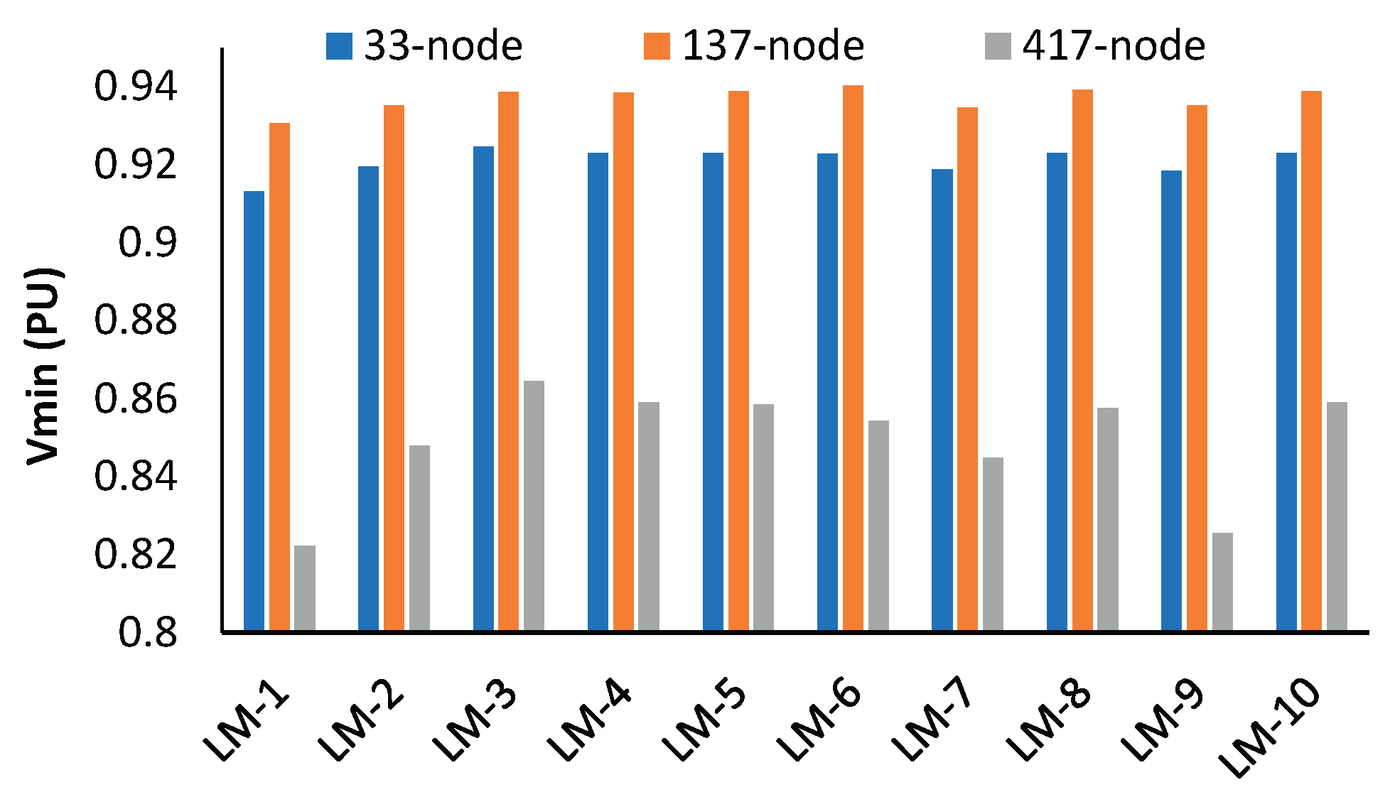
Figure 11.
Objective function under different LMs with no BES.
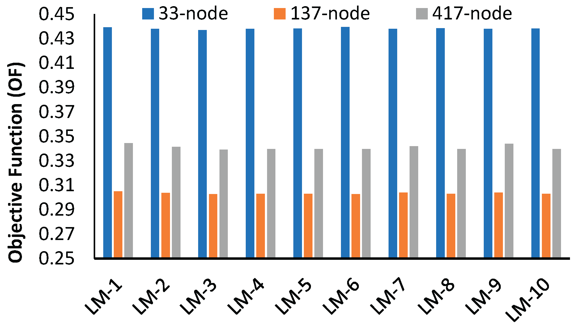
For the 137-node network, the Vmin and PLmax are obtained for LM-1. Also, LImin1 and LImin2 are maximum in LM-3 and minimum in LM-1. However, the minimum value of RImax is 1.6545, and it is in LM-3. For the 417-node network, the minimum voltage and maximum loss are found to be 0.8919 pu and 57.18 kW in LM-1, respectively. Conversely, the minimum voltage profile of the 137-node network is better as compared to other networks, i.e. 33- and 417-node networks, as shown in Figure 10. However, even though the voltage profile of the 137-node network is significantly high, the objective function of 33-node network is considerably higher than other networks therefore, it can be noticed that the 33-node network is more energy efficient in its base configuration when no BES is integrated as compared to the 137- and 417-node systems.
Table 4 shows the EEP of 33-, 137- and 417-node RDNs with BES as a load. The optimal location of BES as a load is obtained at different nodes for different LMs. EEP of RDNs is evaluated based on minimum voltage, power loss, loadability and reliability. For a 33-node network, the minimum voltage and maximum loss are found to be 0.8998 pu and 56.65 kW in LM-1, whereas the maximum values of LImin1 and LImin2 are 3.11 and 14.54 in LM-4 and LM-3, respectively. This is due to the fact that the BES nodes in these LMs are different. The minimum voltage profile is improved in the 137-node network compared to 33-and 417-node networks, as shown in Figure 12. Also, the maximum objective function value is found in LM-9 for 33-node, LM-1 for 137-node and LM-2 for 417-node networks, as shown in Figure 13.
Table 5 shows the EEP of 33-, 137- and 417-node RDNs with BES as a source. Here, the optimal location of BES as a source is obtained at different nodes across all LMs and the EEP of RDNs is found to be improved differently. Consequently, the optimization performed for small and medium networks cannot be directly implemented for large RDNs.
Further, for the 33-node system, Vmin and PLmax are found to be 0.9159 pu and 47.46 kW in LM-1, whereas the maximum values of LImin1 and LImin2 are 16.47 and 3.86 in LM-6, respectively. Conversely, the maximum value of RImax and OF for the 33- and 137-node networks is obtained in LM-1, whereas for the 417-node network, the RImax is found in LM-1, and the maximum value of OF is in LM-9. However, Figure 14 and Figure 15 show the variation in minimum voltage profile and OF across all LMs where Vmin is high in a 137-node followed by a 33-node network, but OF is minimum in the 137-node network. The EP pattern with BES as a load and source is entirely different. Also, it can be noticed that the location of BES as a source is found at different nodes across all LMs. This implies that electric vehicle charging and discharging stations should be different to improve the EEP in power delivery.
6.2. EEP of RDNs in Optimal Configuration
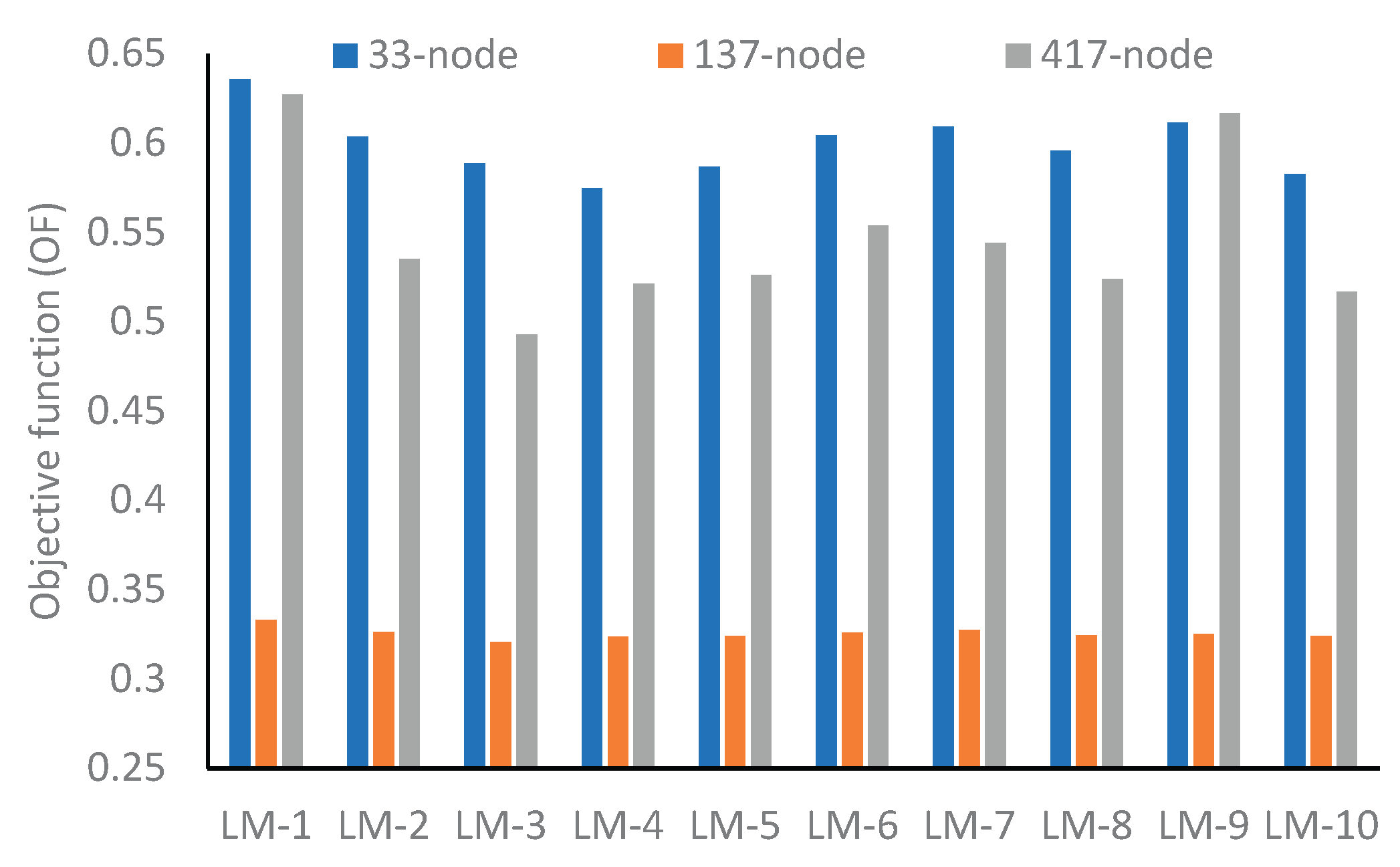
This section evaluates the EEP of 33-, 137- and 417-node in optimal configuration with and without BES. Table 6 shows the EEP of RDNs with no BES. The optimal configuration is obtained with LM-1, and the EEP of the resulting configuration is investigated across all LMs for simplicity. Otherwise, there may be different configurations if optimization is performed for each LM exclusively [17]. Here, a lower value of Vmin is obtained in LM-1 across all RDNs under consideration. However, the Vmin profile of the 137-node network is again found to be improved, whereas, in optimal configuration, the Vmin profile of the 417-node network has improved as compared to the 33-node network, which was improved in the case of base configuration. This implies that the scope of improvement in voltage profile is more significant in large networks than in smaller ones. Additionally, the objective function value of 33- and 417-node networks has improved significantly, whereas, for the 137-node network, the improvement is marginal even though the voltage profile of this network is found to have significantly improved as compared to any other networks, as shown in Table 6 and Figure 16 and Figure 17.
Table 7 shows the EEP of RDNs in optimal configuration with BES as a load. Here, the best position of the BES in each network under the optimal configuration is examined, and EEP parameters under different LMs have been analyzed. The optimal location of BES in optimal configuration is found to be different to that of the base configuration, as shown in Table 7, which in turn affects the EEP of RDNs differently in different LMs. The size of BES as a load and source is kept the same in optimal configuration as well.
From test results, it can be observed that, for a 33-node network, the Vmin is 0.9337 pu in LM-3, and the minimum value of PLmax is 23.05 kW in LM-1 and LM-6, respectively. For the 137-node network, Vmin is 0.9589 pu in LM-1, and the minimum value of PLmaxis 19.0 kW in LM-3. Similarly, for the 417-node network, Vmin is 0.9549 pu, LImin1 is 5.67, and LImin2 is 14.07 in LM-1, whereas the minimum value of PLmax is found to be 49.16 kW in LM-3.
Conversely, Table 8 shows the EEP of 33-, 137- and 417-node networks with BES as a source. In case BES is a source, the voltage profile, power loss, and reliability follow the different patterns when BES works as a load, as discussed above. Here, it can be noticed that the Vmin profile in LM-3 for a 33-node network with BES as a load is 0.9337 pu and source as is 0.9439 pu, which has significantly improved as compared with any other LMs and across all networks as shown in Figure 18. Further, with BES as a source, the objective function of the 33-node network has improved significantly compared to the 137- and 417-node networks, as shown in Figure 19.
Here, it can be observed that the EEP of RDNs in base and their optimal configuration varies significantly across all LMs. In practice, LMs, except LM-1, are voltage-dependent and integration of BES as a load or source can affect the system voltage profile differently. This requires further investigation of EEP when the integration of BES as a load or source is coordinated with a change in network topology, which is presented in the next section
6.3. EEP of RDNs in Coordinated Configuration
With changes in loading patterns, the distribution utilities perform network reconfiguration (NR). NR is a discrete problem with no fixed solution; therefore, heuristics approaches play an important role in such optimization.
In the proposed work, optimization is performed using HSA for BES integration in coordination with configuration management. The optimization results in coordination are presented in Table 9 and Table 10 when BES works as a load and source, respectively. Here, the result shows that the optimal location of BES is found to vary with every change in network topology, which, in turn, with the same size of BES, affects the EEP significantly. For a 33-node network, when BES is a load, the value of PLmax varies marginally, whereas, for a 137-node network, it varies significantly across all LMs to obtain a coordinated configuration, as shown in Table 9.
From the test result of coordinated configuration with BES as a load, as shown in Table 9, the EEP of RDNs is evaluated in terms of line loss, minimum voltage profile, loadability and reliability of supplying power. From Figure 22, it can be observed that the minimum voltage of 33-node is high in LM-6 and LM-8, whereas for 137- and 417-node networks, it is high in LM-10 and LM-3, respectively. However, when the Vmin profile is compared across different RDNs, it is found to improve in the 417-node network in LM-2, LM-3, LM-5, LM-8, and LM-9. On the other hand, for optimal configuration, the voltage profile of the 137-node network was improved as compared to any other networks under consideration, as shown in Figure 16, Figure 18 and Figure 20. Similarly, the OF value for the base and optimal configuration is found to improve in the 33-node network, whereas for the 417-node network, it is found to improve in LM-9, as shown in Figure 23. This implies that the EEP of RDNs under different loading conditions may not be very uniform from small to large networks. Rather, they need to be evaluated with multi-objective functions.
Figure 20.
Voltage profile under different LMs with BES as a source.
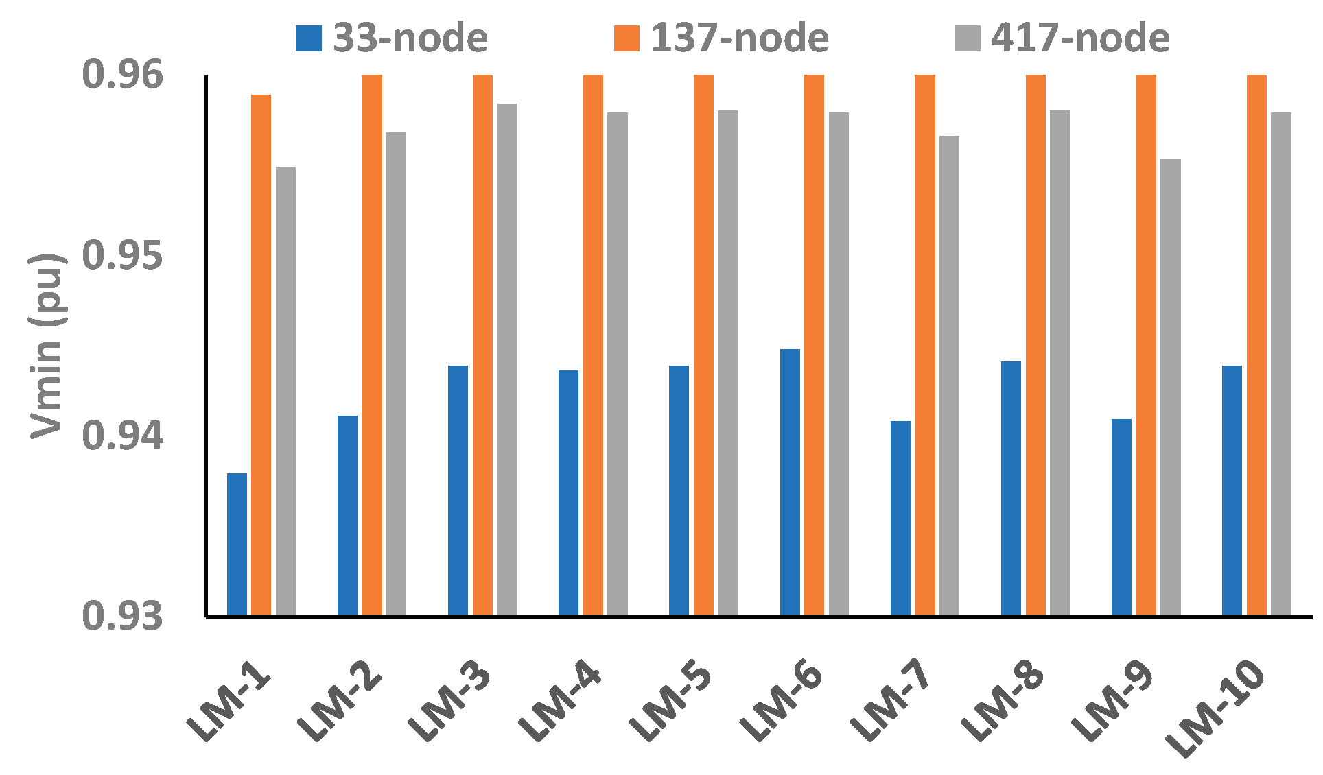
Figure 21.
Objective function under different LMs with BES as a source.
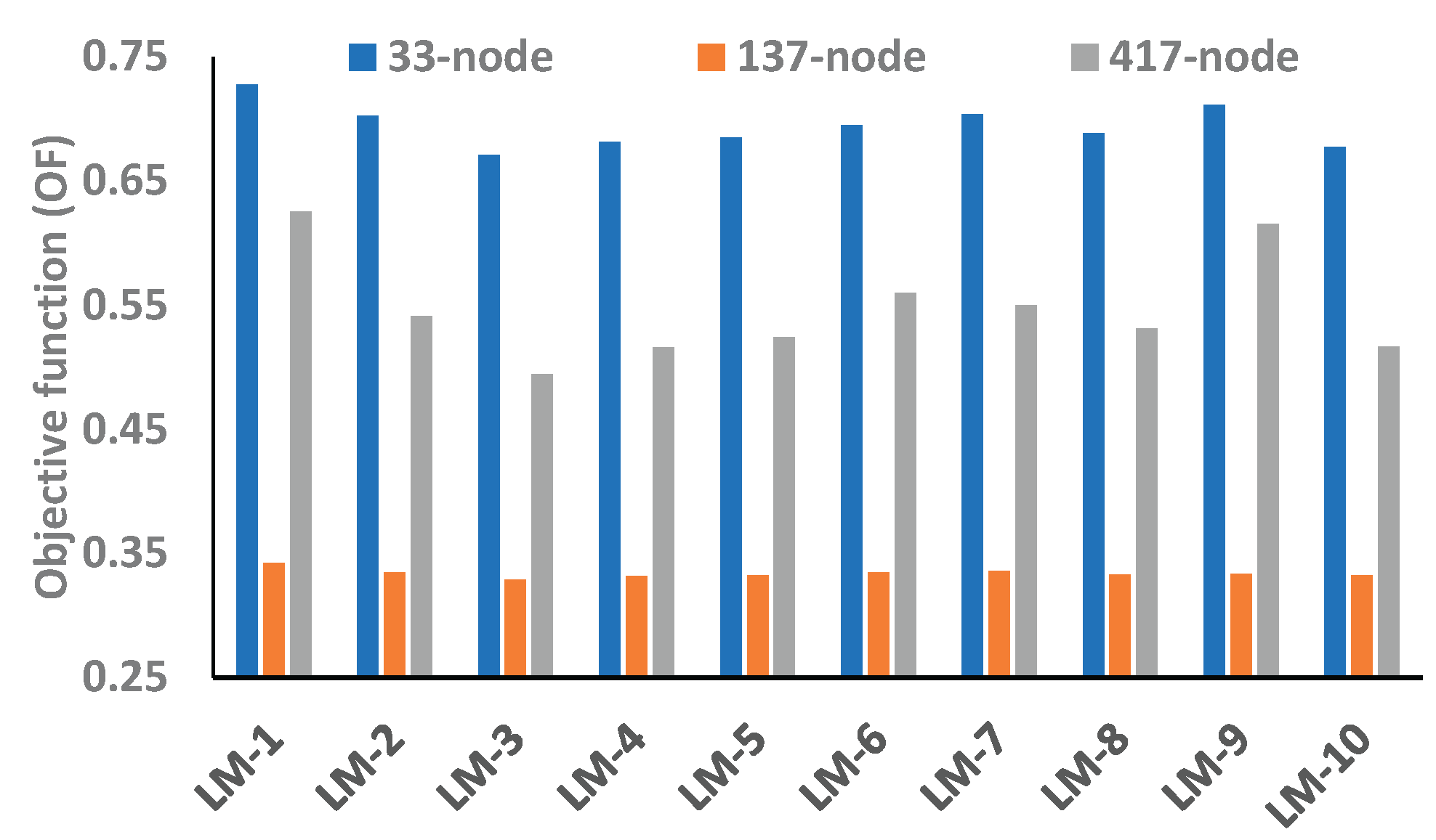
Figure 22.
Voltage profile under different LMs with BES as a load.
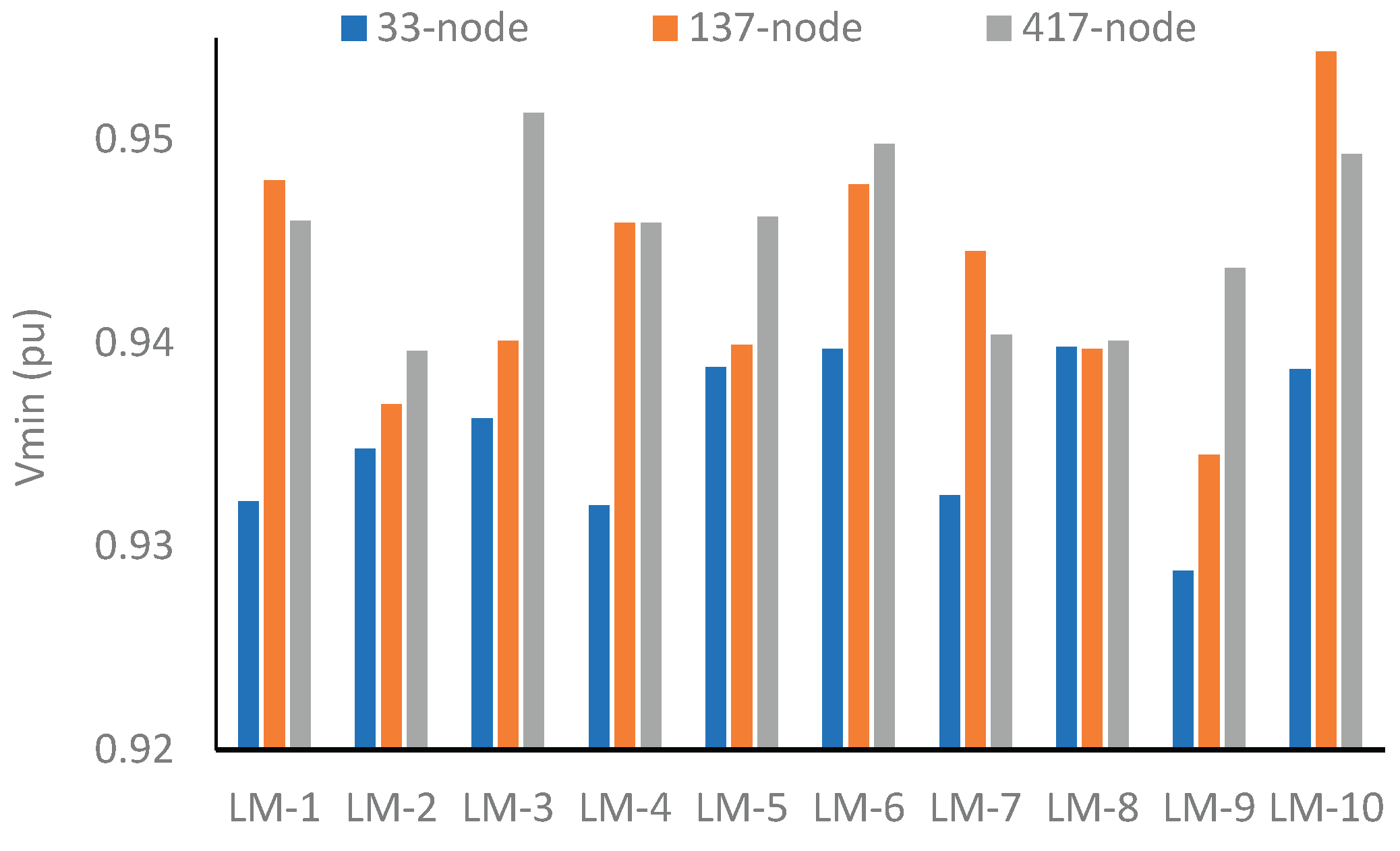
Figure 23.
Objective function under different LMs with BES as a load.
Conversely, Table 10 shows the EEP of RDNs when BES works as a source. Here, it can be noticed that the optimal location of BES is different from that of BES as a load. As a result, the Vmin, PLmax, LImin1 and LImin2 are found to be different. Here, the Vmin profile of the 137-node network is found to be improved in LM-1, LM-2 and LM-6 only, which was enhanced in all LMs in the case of base and optimal configuration. Also, the Vmin profile of the 137-node network in LM-7 and LM-9 is significantly low as compared to any other networks. However, when the Vmin profile is compared across different RDNs, it is found improved in the 417-node network in LM-3, LM-4, LM-5, LM-8, LM-9 and LM-10, as shown in Figure 24. Further, as shown in Figure 25, with BES as the source, OF is improved in the 33-node network across all LMs. Table A1 and Table A2 show the coordinated configuration of the 137- and 417-node networks, respectively. The coordinated configuration of the 33-node network is described in Table 9 and Table 10.
Figure 26 shows that the objective function (OF) is maximum in the coordinated configuration in LM-3, LM-6 and LM-8 with BES as a load, whereas for this network with BES as the source, OF is maximum in all LMs in an optimal configuration. On the other hand, OF for the 137-node network is maximum in optimal configuration in LM-1 only with BES as a load. For BES as a source, OF is the maximum in coordinated configuration for all LMs. However, for the 417-node network, OF is maximum in LM-5, LM9 and LM-10 in optimal configuration with BES as a load, whereas OF is maximum in coordinated configuration across all LMs with BES as a source. From the result, it can be observed that the energy efficiency performance of RDNs, when tested with a single objective for the small network, cannot be straightway implemented. In practice, for the large network for a truly energy-efficient operation under different operating scenarios of loading patterns, the optimization needs to be performed in coordination with multi=objective functions.
6.4. Computational Performance of Proposed Approach for Loss Minimization
The computational performance of the proposed approach is evaluated on six different RDNs available in the literature. However, a detailed EPP analysis is performed for three RDNs, i.e., small, medium and large networks. These findings also show how energy storage systems can affect the EEP of small, medium, and large networks when they work as a load or source under different operating scenarios and different loading patterns.
For the robustness of the proposed approach, the algorithm is run 10 times with 300 iterations in each run. The minimum and maximum value of the objective function, i.e., loss minimization, is evaluated with a probability of imposing node voltage from 0.0 to 1.0. The results of 33-, 137- and 417-node are shown in Table 11 with their minimum computational time out of 10 runs. Here, it can be noticed that the minimum CT for 33-node is 0.72 sec when PINV is 0.8, for 137-node CT is 5.72 sec when PINV is 0.7 and for 417-node network CT is 22.39 sec when PINV is 0.8. However, Table 12 shows the average CT of 3 runs when PINV is fixed as 0.8. Also, here, it can be observed that the average CT of a 119-node network is higher than that of a 137-node network because of the greater number of parallel paths formed while reconfiguring the network topology, which makes the convergence sluggish. However, the overall performance of the proposed approach is found to be improved as compared to the existing approaches in terms of the CT obtained with a 2.5 GHz, Intel i5 processor, 4GB RAM and 64-bit system.
The CT of six different RDNs, from smallest to largest, is presented in this work. Optimization is performed for loss minimization to compare the convergence performance of the proposed approach. Figure 27 shows the convergence characteristics of the proposed approach implemented through 33-, 69-, 85-, 119-, 137- and 417-node radial networks. Here, it can be observed that the convergence of the 33- and 69-node networks has occurred even in less than 100 iterations, whereas the rate of convergence is highest in the 69-node network and slowest in the 119-node network, as shown in Figure 27. Further, the CT in existing work is measured with an Intel i7 processor [29], and there is no consistency in the convergence as the small network has more CT. Also, for the 417-node network, the CT has inclined exponentially. Conversely, in the proposed work, the CT is consistent, and the rate of convergence is high except for the 119-node network, which is due to the sluggish characteristics of this network, as shown in Figure 27.
7. Conclusions
The proposed work presented the energy efficiency performance (EEP) of small, medium and large RDNs with battery energy storage (BES) as a load and source exclusively. The performance matrix includes node voltage profile, power losses, loadability, load balancing, reliability and convergence rate. For the load flow solution, a voltage iterative approach is adopted, whereas the optimization is performed using a modified harmony search algorithm (HSA). Here, EEP is evaluated for base, optimal and coordinated configuration under different probabilistic loading patterns (PLP). The loading patterns are voltage-dependent and hence the performance indices; therefore, while reconfiguring the network topology, a probability of imposing node voltage (PINV) is framed and implemented for every new selection of solution vector of HSA from global solution during random selection. For different PLPs, the EEP of radial networks under consideration is found to vary differently with BES as a load and source. In small networks, the EEP of the optimal configuration is higher than that of the corresponding base and coordinated configurations. However, in large networks, the EEP of the coordinated configuration shows improvement. Therefore, the existing approach of optimization for the small networks cannot be directly implemented on the large network. Rather, it requires a multi-objective approach for the energy-efficient operation of RDNs. The proposed work additionally demonstrated the benefit of different values for these characteristics in guiding the best allocation strategies for BES under different loading patterns since the optimal configuration and BES allocation as a load or source are found to be different. Further, implementing DSM and DVR integration can also affect EEP differently and needs to be addressed in future works. Moreover, the proposed approach benefits customers and utilities and helps decision-making for sustainable, reliable, and efficient distribution networks while delivering power.
Author Contributions
“Conceptualization, P.K. and P.K.; methodology, P.K and P.K.; software, P.K.; validation, P.K., and G.K.; formal analysis, P.K.; investigation, P.K and P.K.; resources, P.K.; data curation, P.K. and G.K.; writing—original draft preparation, P.K. and P.K.; writing—review and editing, P.K. and G.K.; visualization, P.K.; supervision, P.K. and G.K. All authors have read and agreed to the published version of the manuscript.
Funding
This research received no external funding.
Data Availability Statement
In the proposed research generalized test system data is used which is available in existing literatures.
Acknowledgments
NA
Conflicts of Interest
The authors declare no conflicts of interest.
Abbreviations
The following abbreviations are used in this manuscript:
| EEP | Energy efficiency performance |
| objective function | |
| RDNs | Radial distribution networks |
| PLP | Probabilistic loading patterns |
| LM | Load model |
| CT | computational time |
| RP | Radial paths |
| HSV | Harmony solution vector |
| HSA | Harmony search algorithm |
| HMCR | Harmony memory consideration rate |
| HMS | Harmony memory size |
| PAR | Pitch adjustment rate |
| BW | Band width |
| HM | Harmony memory |
| MI | Maximum improvisation |
| NVI | Node voltage index |
| NDI | Node demand index |
| NLI | Node loadability index |
| NRI | Node reliability index |
| NPI | Node power loss index |
| is the respective index number in OF | |
| penalty factor for power loss on OF | |
| Set of total, connected branches and tie-lines. | |
| Voltage at ith and jth node | |
| Active, reactive and apparent load demand at ith node | |
| Branch current between ith and jth node | |
| Nominal value of active and reactive load demand at ith node | |
| min. & max. value of ST at any node | |
| Resistance and reactance of branch between ith and jth node | |
| α, β | Voltage exponent of active and reactive power |
| Equivalent R, X and Z between source and jth node | |
| New solution vector | |
| Active & reactive loss of branch between ith and jth node | |
| n | Number of nodes |
| Set of sending & receiving end nodes of branches | |
| SOC, SOCi-1 | Present & previous state of charge |
| Set of sending & receiving end nodes of | |
| ηc, ηd | Charge & discharge efficiency of a battery |
| Set of sending & receiving end nodes of tie-lines | |
| Energy not supplied | |
| Total active, reactive & apparent demand at a node | |
| repair time & failure rate, resp. | |
| Min. and Max. value of ST in a given topology | |
| System average interruption duration index | |
| Generated active and reactive power at ith node | |
| System average interruption frequency index | |
| BES, BESmin, BEXmax | Battery energy storage, and its min & max. value |
| ∆t | Time for discharge or charge of battery |
| Reliability index, min. & max. value of RI | |
| Reliability index for criterion 1 and 2, resp. | |
| Loadability index, min. and max. value of LI | |
| , | Loadability index for criterion 1 and 2, resp. |
| Min. and max. value of line power loss | |
| Charging and discharging power of battery |
Appendix A

Table A1.
Coordination configuration of the network with BES as a load.
| Coordinated configuration of 137-node network with BES as a load | |
| LM-1 | 8 138 139 39 141 142 143 144 145 146 85 148 149 91 151 152 97 108 127 129 136 |
| LM-2 | 8 21 139 28 141 142 55 144 145 146 147 148 149 150 151 152 153 107 127 129 157 |
| LM-3 | 8 21 139 28 141 142 56 144 145 146 147 148 149 91 151 152 97 107 127 129 157 |
| LM-4 | 8 21 139 36 141 142 143 144 145 146 147 148 149 91 151 152 97 107 127 129 136 |
| LM-5 | 8 21 139 28 141 51 143 119 145 146 147 148 149 91 151 152 153 107 127 156 157 |
| LM-6 | 8 21 16 32 141 50 54 144 145 146 85 148 149 150 151 152 97 107 155 129 157 |
| LM-7 | 8 21 16 32 141 142 56 144 145 146 85 148 149 150 151 152 153 107 127 156 136 |
| LM-8 | 8 21 16 28 141 50 143 144 145 146 147 148 149 150 151 152 153 107 155 129 157 |
| LM-9 | 8 21 139 28 141 142 143 144 145 146 147 148 149 150 151 152 153 108 127 129 136 |
| LM-10 | 8 10 139 140 141 142 54 119 145 146 85 148 149 91 151 152 153 108 127 129 136 |
| Coordinated configuration of 417-node network with BES as a load | |
| LM-1 | 7 15 17 21 3 35 32 55 56 61 54 74 87 88 95 89 98 112 116 137 147 150 107 156 149 159 164 169 170 179 385 196 200 214 215 257 255 279 283 302 322 323 359 363 370 393 396 397 401 403 404 417 428 432 433 438 447 450 467 |
| LM-2 | 7 212 17 21 3 23 32 55 56 61 54 74 87 88 95 77 98 108 116 145 147 150 151 156 153 159 164 169 170 230 377 196 200 214 215 257 255 271 283 302 322 323 359 363 370 393 396 397 401 403 404 417 428 432 437 442 455 450 467 |
| LM-3 | 7 15 17 18 3 31 32 51 56 61 70 74 127 88 95 97 98 112 116 141 143 146 151 156 153 175 164 169 170 179 385 196 200 214 215 257 255 279 283 302 322 323 359 363 370 393 396 397 401 403 404 417 428 436 433 438 455 450 467 |
| LM-4 | 7 15 17 14 3 16 32 51 44 61 58 74 91 88 95 77 94 112 116 141 143 150 151 156 153 159 164 169 170 179 381 196 200 210 215 257 255 279 283 302 322 323 359 363 370 393 396 397 401 427 404 417 428 432 437 438 447 450 467 |
| LM-5 | 7 15 13 25 22 20 32 43 56 61 30 74 91 88 95 9 98 112 116 129 143 150 151 156 149 159 164 169 174 179 385 188 200 214 215 257 255 279 283 302 322 323 359 363 370 393 396 397 401 427 404 417 424 436 437 438 447 450 467 |
| LM-6 | 7 212 17 18 216 31 32 55 44 61 54 74 91 88 95 85 98 112 116 137 147 150 151 156 153 171 164 169 170 179 385 196 200 210 215 257 255 279 283 302 322 323 359 363 370 393 396 397 401 427 404 417 424 436 437 438 447 450 467 |
| LM-7 | 7 15 17 21 3 20 32 51 60 61 54 74 87 88 95 89 98 112 116 141 147 150 119 132 149 159 384 169 170 179 180 400 200 214 215 257 255 279 283 302 322 323 359 363 370 393 396 397 401 403 404 417 428 432 433 438 455 450 467 |
| LM-8 | 7 212 17 25 216 27 32 55 56 61 54 74 87 88 95 81 98 112 116 141 143 146 151 156 149 159 164 169 170 242 377 196 200 210 215 257 255 279 283 302 322 323 359 363 370 393 396 397 401 403 404 417 424 436 433 438 447 450 467 |
| LM-9 | 7 212 13 14 22 20 32 47 60 61 30 74 91 88 95 101 94 112 116 145 143 150 151 156 149 159 164 169 170 179 180 196 200 214 215 257 255 271 283 302 322 323 359 363 370 393 396 397 401 403 404 417 424 432 433 438 447 450 467 |
| LM-10 | 7 15 13 18 3 23 32 51 56 61 54 74 87 88 95 9 98 112 116 145 139 150 151 156 153 171 164 169 174 179 180 196 200 214 215 257 255 275 283 302 322 323 359 363 370 393 396 397 401 403 404 417 428 436 437 438 455 450 467 |
Table A2.
Coordination configuration of the network with BES as a source.
| Coordinated configuration of 137-node network with BES as a source | |
| LM-1 | 8 138 139 140 141 51 54 119 145 146 85 148 149 91 151 152 153 108 127 156 157 |
| LM-2 | 8 10 139 140 141 142 54 144 145 146 85 148 149 91 151 152 153 108 127 129 157 |
| LM-3 | 8 21 139 27 141 142 143 119 145 146 147 148 149 91 151 152 153 107 155 129 136 |
| LM-4 | 8 21 139 27 141 50 143 144 145 146 147 148 149 91 151 152 153 107 155 129 157 |
| LM-5 | 8 21 139 28 141 142 143 119 145 146 147 148 149 91 151 152 153 107 155 156 136 |
| LM-6 | 8 21 16 32 141 142 56 144 145 146 85 148 149 91 151 152 153 107 155 156 157 |
| LM-7 | 8 21 139 27 141 50 55 144 145 146 147 148 149 91 151 152 120 107 127 129 157 |
| LM-8 | 8 21 139 28 141 142 56 63 145 146 147 148 149 91 151 152 153 107 127 129 157 |
| LM-9 | 8 21 139 28 141 142 54 119 145 146 147 148 149 91 151 152 97 107 127 156 157 |
| LM-10 | 8 21 139 27 141 50 143 144 145 146 147 148 149 150 151 152 153 108 155 129 157 |
| Coordinated configuration of 417-node network with BES as a source | |
| LM-1 | 7 212 17 21 22 35 32 51 56 61 30 74 127 88 95 85 98 112 116 137 143 150 107 156 157 159 164 169 170 179 385 196 200 210 215 257 255 275 283 302 322 323 359 363 370 393 396 397 401 403 404 417 424 440 437 438 447 450 467 |
| LM-2 | 7 15 17 18 3 27 32 43 60 61 62 74 91 88 95 101 98 112 116 137 139 142 151 156 157 159 164 169 170 179 377 196 200 214 215 257 255 267 283 302 322 323 359 363 370 393 396 397 401 427 404 417 428 432 437 438 447 450 467 |
| LM-3 | 7 212 17 21 216 35 32 51 60 61 58 74 127 88 95 77 98 112 116 141 139 150 107 156 157 159 164 169 174 179 381 188 200 210 215 257 255 279 283 302 322 323 359 363 370 393 396 397 401 427 404 417 424 432 433 438 447 450 467 |
| LM-4 | 7 212 13 25 22 16 32 55 44 61 54 74 91 88 95 77 98 112 116 145 143 150 103 156 157 159 164 169 174 179 180 196 200 214 215 257 255 279 283 302 322 323 359 363 370 393 396 397 401 403 404 417 424 432 433 438 447 450 467 |
| LM-5 | 7 15 17 14 3 27 32 51 60 61 54 74 127 88 95 89 98 112 116 145 143 142 151 156 153 159 164 169 178 179 180 196 200 214 215 257 255 279 283 302 322 323 359 363 370 393 396 397 401 427 404 417 424 440 437 438 455 450 467 |
| LM-6 | 7 212 17 14 22 20 32 47 56 61 58 74 87 88 95 97 102 112 116 129 147 150 107 156 149 159 164 169 170 179 381 188 200 210 215 257 255 275 283 302 322 323 359 363 370 393 396 397 401 403 404 417 424 432 433 438 447 450 467 |
| LM-7 | 7 212 17 14 216 16 32 51 56 61 30 74 91 88 95 81 94 112 116 141 147 150 107 156 157 159 164 169 170 179 381 188 200 214 215 257 255 267 283 302 322 323 359 363 370 393 396 397 401 427 404 417 428 440 437 438 447 450 467 |
| LM-8 | 7 15 17 21 22 23 32 43 44 61 54 74 87 88 95 97 98 112 116 129 147 150 107 156 153 159 164 169 170 179 381 196 200 214 215 257 255 271 283 302 322 323 359 363 370 393 396 397 401 427 404 417 428 436 437 438 447 450 467 |
| LM-9 | 7 15 17 25 3 35 32 55 44 61 70 74 91 88 95 77 98 100 116 137 147 150 151 156 149 159 164 169 170 179 377 196 200 210 215 257 255 267 283 302 322 323 359 363 370 393 396 397 401 427 404 417 428 436 437 438 447 450 467 |
| LM-10 | 7 212 17 25 3 16 32 55 56 61 54 74 87 88 95 77 94 108 116 145 147 146 107 156 153 159 164 169 170 179 381 188 200 214 215 257 255 279 283 302 322 323 359 363 370 393 396 397 401 403 404 417 424 432 433 442 447 450 467 |
References
- Kumar, P.; Singh, S. Comprehensive stability analysis of radial distribution system with load growth. In Proceedings of the 2014 IEEE 6th India International Conference on Power Electronics (IICPE), Kurukshetra, India, 8–10 December 2014; IEEE: Piscataway, NJ, USA, 2014; pp. 1–6. [Google Scholar]
- Ihara, S.; Tani, S.M.; Tomiyama, K. Residential load characteristics observed at KEPCO power system. IEEE Trans on Power Systems 1994, 9, 1092–1101. [Google Scholar] [CrossRef]
- Kumar, P.; Nikolovski, S.; Ali, I.; Thomas, M.S.; Ahuja, H. Impact of Electric Vehicles on Energy Efficiency with Energy Boosters in Coordination for Sustainable Energy in Smart Cities. Processes 2022, 10, 1593. [Google Scholar] [CrossRef]
- Kumar, P.; Ali, I.; Thomas, M.S. Energy efficiency analysis of reconfigured distribution system for practical loads. Perspect. Sci. 2016, 8, 498–501. [Google Scholar] [CrossRef]
- Najafabadi, A.M.; Alouani, A.T. Real time parameter identification of composite load model. In Proceedings of the 2013 IEEE Power & Energy Society General Meeting (PESGM), Vancouver, BC, Canada, 21–15 July 2013. [Google Scholar]
- Chakraborty, S.; Bohre, A.K. Planning of Renewable DG with Different Load Modelling. In Proceedings of the 2021 IEEE 2nd International Conference On Electrical Power and Energy Systems (ICEPES), Bhopal, India, 10–11 December 2021; pp. 1–7. [Google Scholar]
- Ali, A.; Abbas, G.; Keerio, M.U. Mirsaeidi, S.; Alshahr, S.; Alshahir, A. Multi-Objective Optimal Siting and Sizing of Distributed Generators and Shunt Capacitors Considering the Effect of Voltage-Dependent Nonlinear Load Models. IEEE Access 2023, 11, 21465–21487. [Google Scholar] [CrossRef]
- Paul, S.; Padhy, N.P. A New Real Time Energy Efficient Management of Radial Unbalance Distribution Networks Through Integration of Load Shedding and CVR. IEEE Transactions on Power Delivery 2022, 37, 2571–2586. [Google Scholar] [CrossRef]
- Saini, P.; Gidwani, L. An investigation for battery energy storage system installation with renewable energy resources in distribution system by considering residential, commercial and industrial load models. Journal of Energy Storage 2022, 45, 103493. [Google Scholar] [CrossRef]
- Jin, X.; Moradi, Z.; Rashidi, R. Optimal Operation of Distributed Generations in Four-Wire Unbalanced Distribution Systems considering Different Models of Loads. Int. Trans. Electr. Energy Syst. 2023, 33. [Google Scholar] [CrossRef]
- Kumar, A.; Deng, Y.; He, X.; Singh, A.R.; Kumar, P.; Bansal, R.C.; Bettayeb, M.; Ghenai, C.; Naidoo, R.M. Impact of demand side management approaches for the enhancement of voltage stability loadability and customer satisfaction index. AppL Energy 2023, 339, 120949. [Google Scholar] [CrossRef]
- Bosisio, A.; Berizzi, A.; Lupis, D.; Morotti, A.; Iannarelli, G.; Greco, B. A Tabu-search-based Algorithm for Distribution Network Restoration to Improve Reliability and Resiliency. J. Mod Power Syst. Clean Energy 2023, 11, 302–311. [Google Scholar] [CrossRef]
- Ali, M.H.; Kamel, S.; Hassan, M.H.; Tostado-Véliz, M.; Zawbaa, H.M. An improved wild horse optimization algorithm for reliability based optimal DG planning of radial distribution networks. Energy Rep. 2022, 8, 582–604. [Google Scholar] [CrossRef]
- Gupta, N.; Swarnkar, A.; Niazi, K.R. Distribution network reconfiguration for power quality and reliability improvement using Genetic Algorithms. I. Journal of Elect. Power & Energy Systems. 2014, 54, 664–671. [Google Scholar]
- Noori, A.; Zhang, Y.; Nouri, N.; Hajivand, M. Multi-Objective Optimal Placement and Sizing of Distribution Static Compensator in Radial Distribution Networks With Variable Residential, Commercial and Industrial Demands Considering Reliability. IEEE Access 2021, 9, 46911–46926. [Google Scholar] [CrossRef]
- Kumar, P.; Ali, I.; Thomas, M.S.; Singh, S. Imposing voltage security and network radiality for reconfiguration of distribution systems using efficient heuristic and meta-heuristic approach. IET Generation, Transmission & Distribution 2017, 11, 2457–2467. [Google Scholar]
- Ali, I.; Thomas, M.S.; Kumar, P. Energy efficient reconfiguration for practical load combinations in distribution systems. IET Gener. Transm. Distrib. 2015, 11, 1051–1060. [Google Scholar] [CrossRef]
- Mendoza, J.E.; Lopez, M.E.; CoelloCoello, C.A.; Lopez, E.A. Micro-genetic multiobjective reconfiguration algorithm considering power losses and reliability indices for medium voltage distribution network. IET Generation, Transmission & Distribution 2009, 9, 825–840. [Google Scholar]
- Jie, W.; Wang, W.; Wang, H.; Zuo, H. Dynamic reconfiguration of multiobjective distribution networks considering DG and EVs based on a novel LDBAS algorithm. IEEE Access 2020, 8, 216873–216893. [Google Scholar]
- Qian, C.; Wang, W.; Wang, H.; Wu, J.; Li, X.; Lan, J. A social beetle swarm algorithm based on grey target decision-making for a multiobjective distribution network reconfiguration considering partition of time intervals. IEEE Access 2020, 8, 204987–205013. [Google Scholar] [CrossRef]
- Kumar, P.; Singh, S. Reconfiguration of RDN with static load models for loss minimization. In Proceedings of the 2014 IEEE international conference on power electronics, drives and energy systems (PEDES); 2014; pp. 1–5. [Google Scholar]
- Meisam, M.; Schmitt, K.; Chamana, M.; Bayne, S.; Jurado, F. Effective Strategies for Distribution Systems Reconfiguration Considering Loads Voltage Dependence. IEEE Transactions on Industry Applications 2023.
- Babanezhaad Shirdar, H.; Ghafouri, A. Optimization of multi-microgrid system operation cost with different energy management tools in the presence of energy storage system. Electric Power Components and Systems 2022, 16–17, 951–971. [Google Scholar] [CrossRef]
- Kumar, P.; Ali, I.; Thomas, M.S.; Singh, S. A coordinated framework of dg allocation and operating strategy in distribution system for configuration management under varying loading patterns. Electric Power Components and Systems 2020, 48, 12–29. [Google Scholar] [CrossRef]
- Sameh, M.A.; Aloukili, A.A.; El-Sharkawy, M.A.; Attia, M.A.; Badr, A. Optimal DGs Siting and Sizing Considering Hybrid Static and Dynamic Loads, and Overloading Conditions. Processe 2022, 12, 12–2713. [Google Scholar] [CrossRef]
- Kumar, B.A.; Agnihotri, G.; Dubey, M. Optimal sizing and sitting of DG with load models using soft computing techniques in practical distribution system. IET Generation, Transmission & Distribution 2016, 10, 2606–2621. [Google Scholar] [CrossRef]
- Cao, B.; Dong, W.; Lv, Z.; Gu, Y.; Singh, S.; Kumar, P. Hybrid microgrid many-objective sizing optimization with fuzzy decision. IEEE Transactions on Fuzzy Systems 2020, 28, 2702–2710. [Google Scholar] [CrossRef]
- Mahdavi, M.; Alhelou, A.H.; Hesamzadeh, M.R. An efficient stochastic reconfiguration model for distribution systems with uncertain loads. IEEE Access 2022, 10, 10640–10652. [Google Scholar] [CrossRef]
- Gallego, L.A.; López-Lezama, J.M.; Carmona, G. A mixed-integer linear programming model for simultaneous optimal reconfiguration and optimal placement of capacitor banks in distribution networks. IEEE Access 2020, 10, 52655–52673. [Google Scholar] [CrossRef]
Figure 1.
A sample network to illustrate radiality.
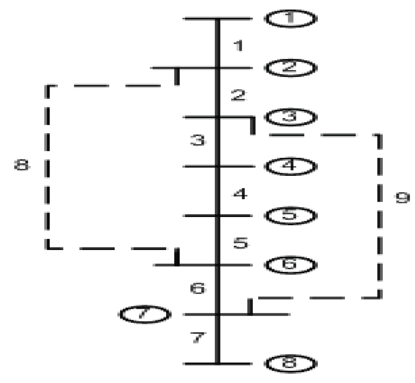
Figure 4.
A sample 33-node RDN.
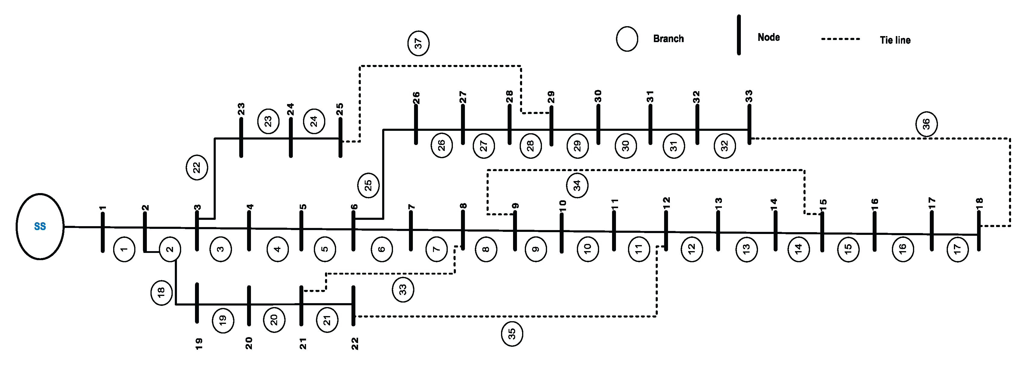
Figure 5.
Node voltage profile of 33-node RDN under different LMs.
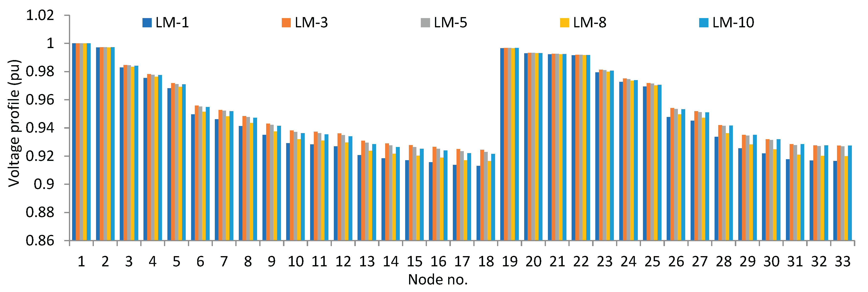
Figure 6.
Active power loss in lines of 33-node RDN under different LMs.
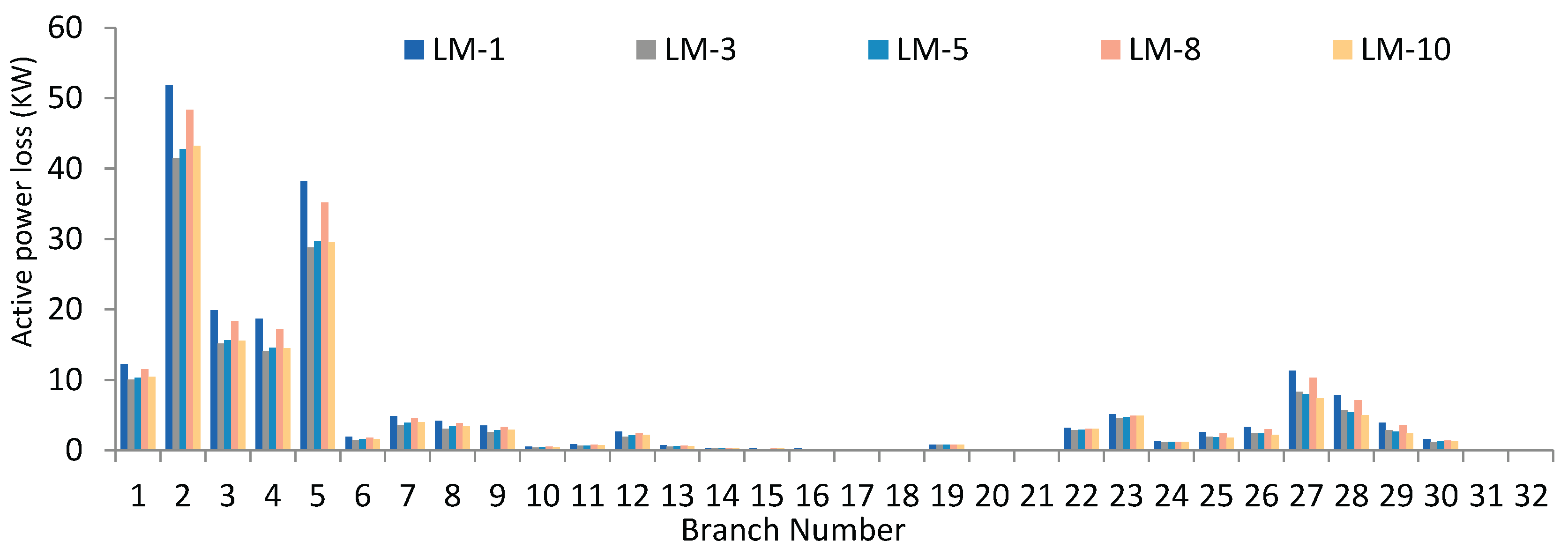
Figure 7.
at each node for 33-nodeRDN under different LMs.
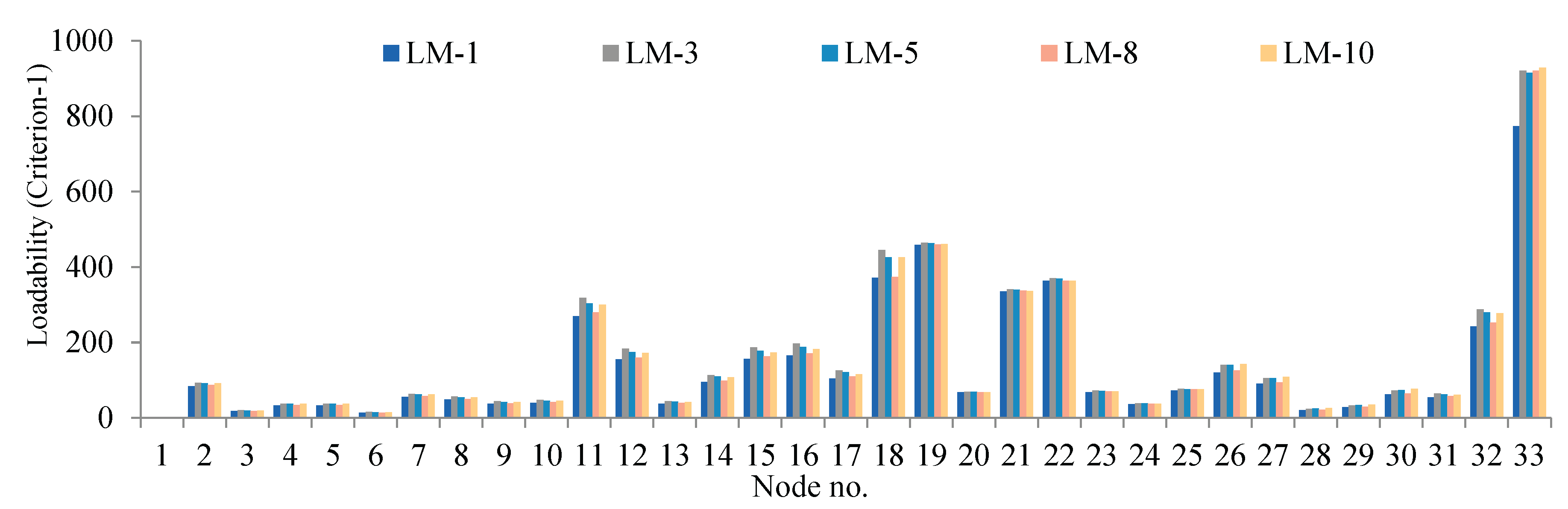
Figure 8.
at each node for 33-node RDN under different LMs.
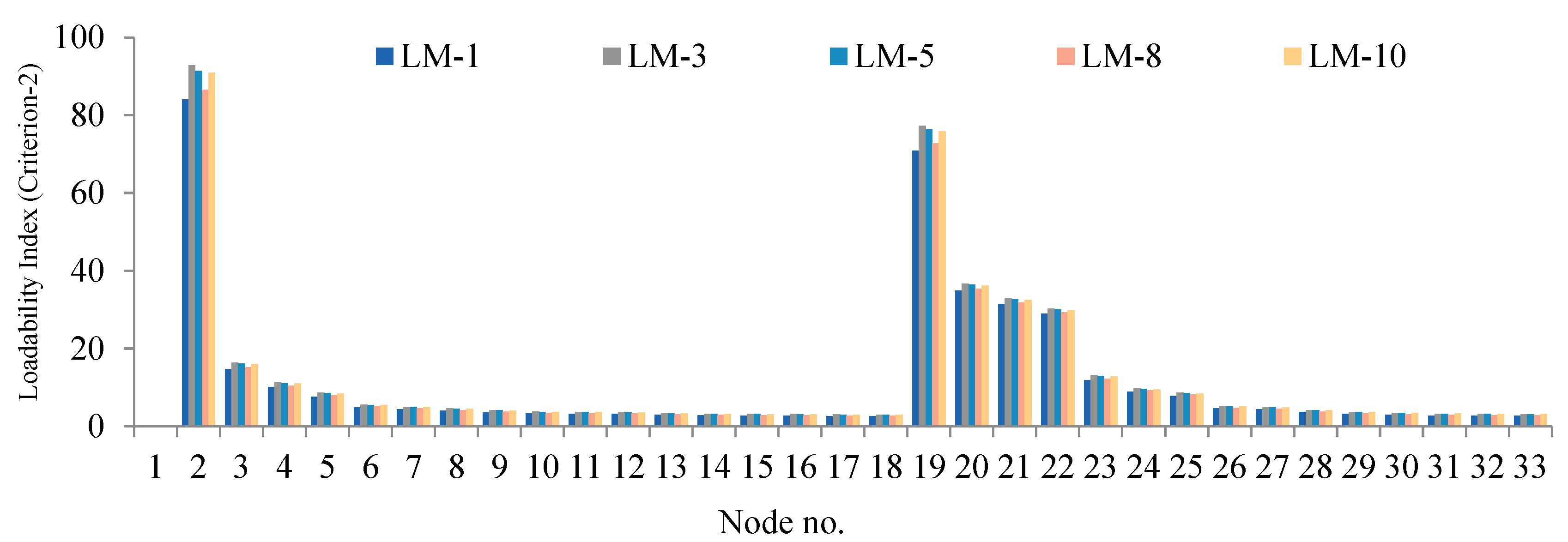
Figure 9.
at each node for 33-node RDN under different LMs.
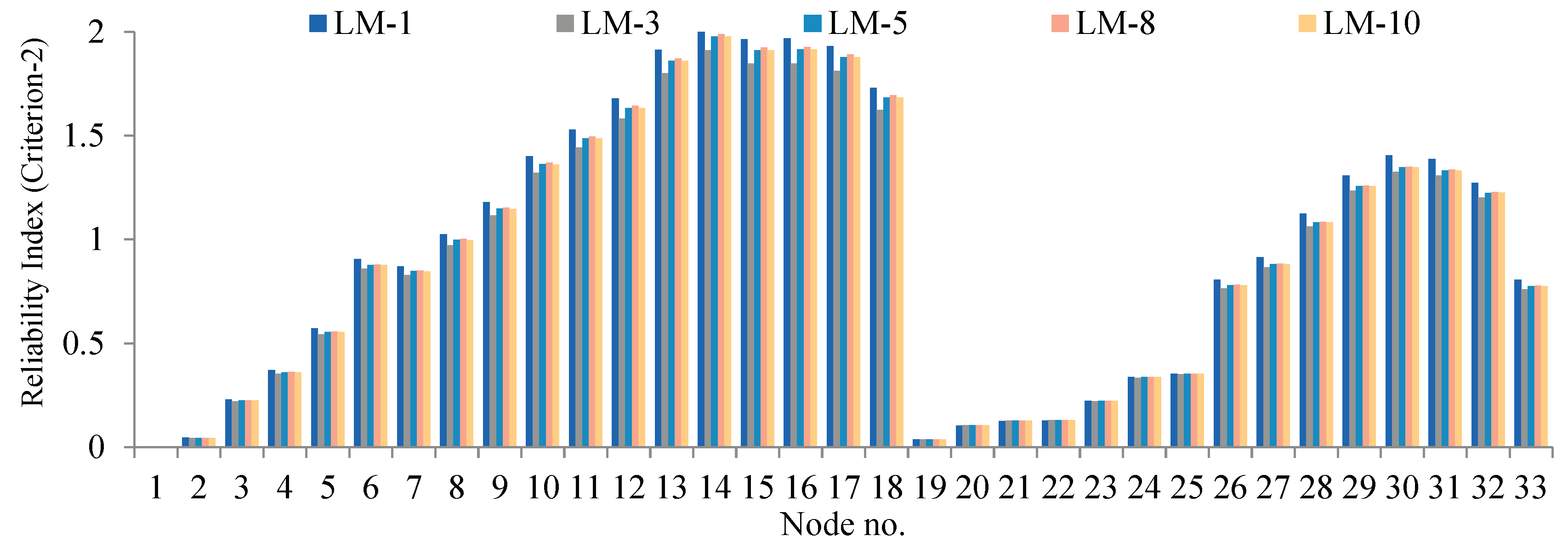
Figure 12.
Voltage profile under different LMs with BES as load.
Figure 13.
Objective function under different LMs with BES as load.
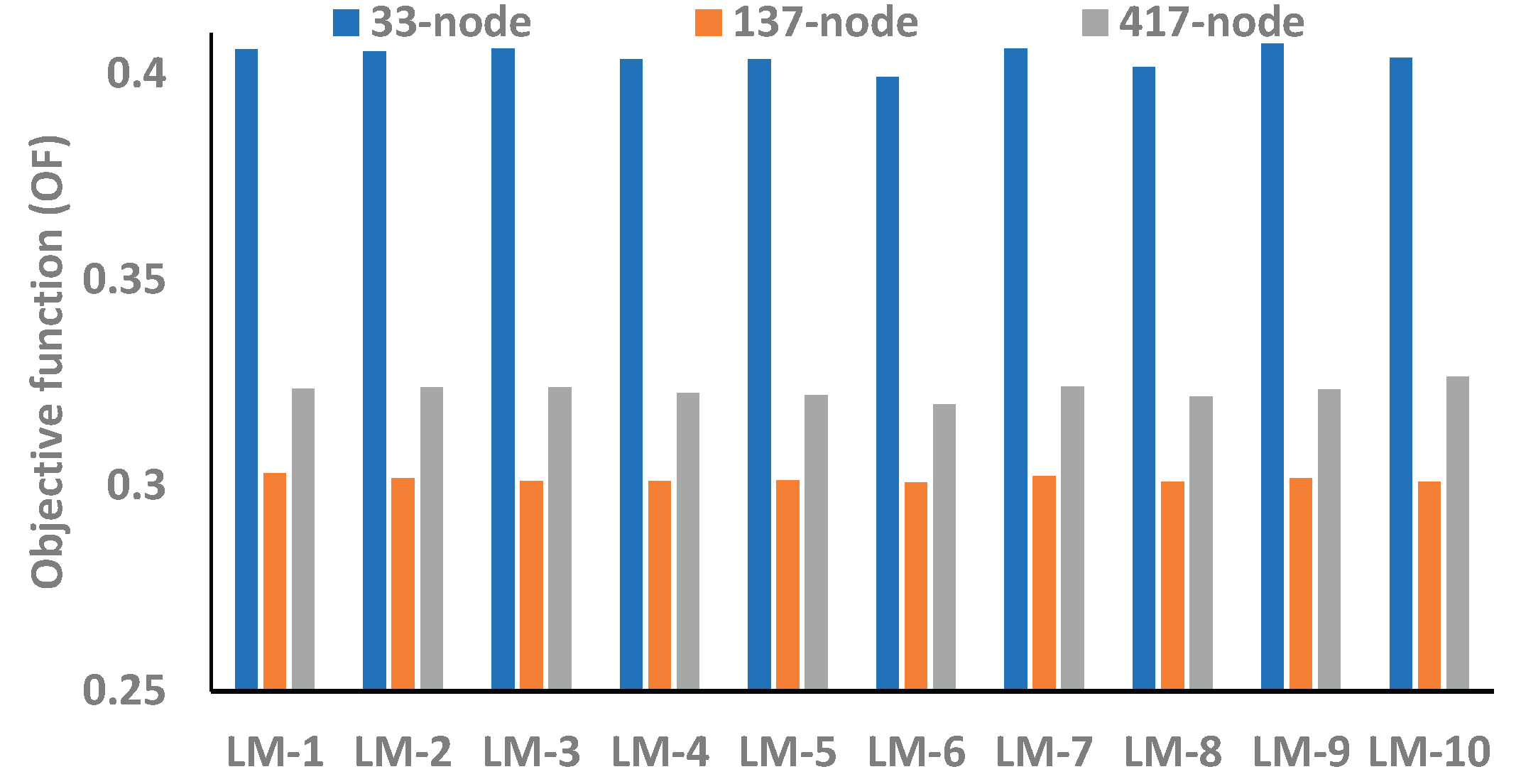
Figure 14.
Voltage profile under different LMs with BES as source.
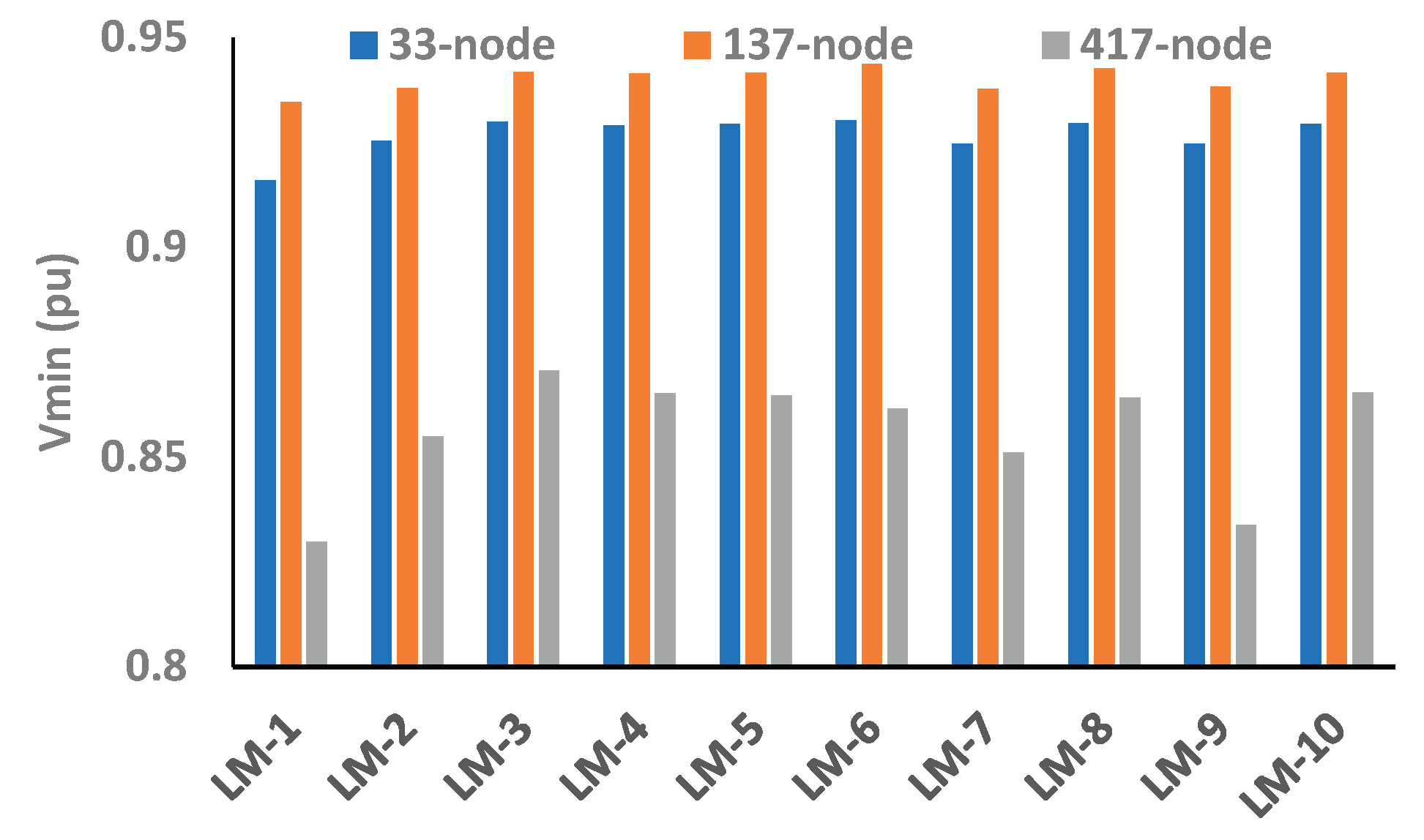
Figure 15.
Objective function under different LMs with BES as source.
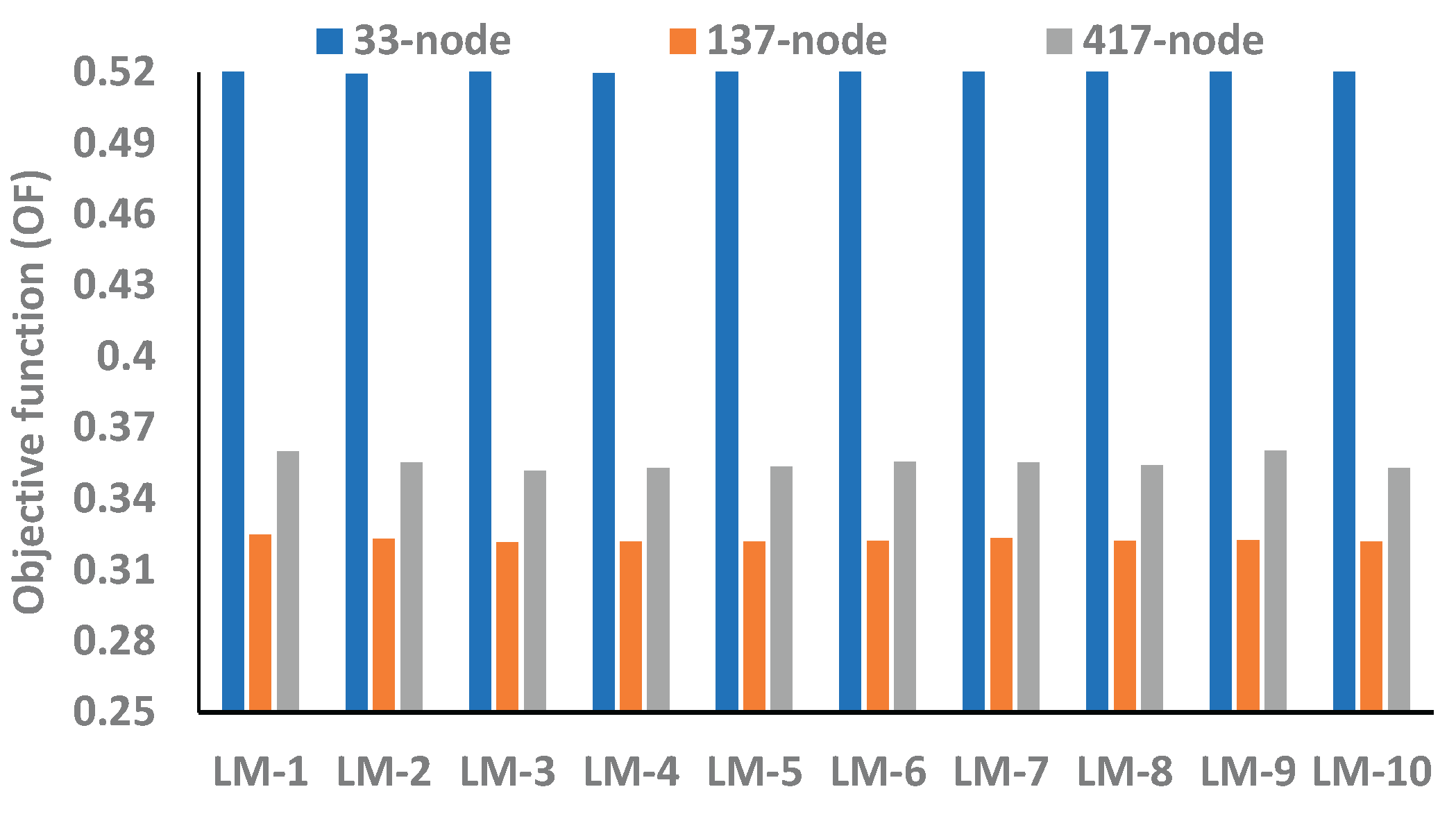
Figure 16.
Voltage profile under different LMs with no BES.
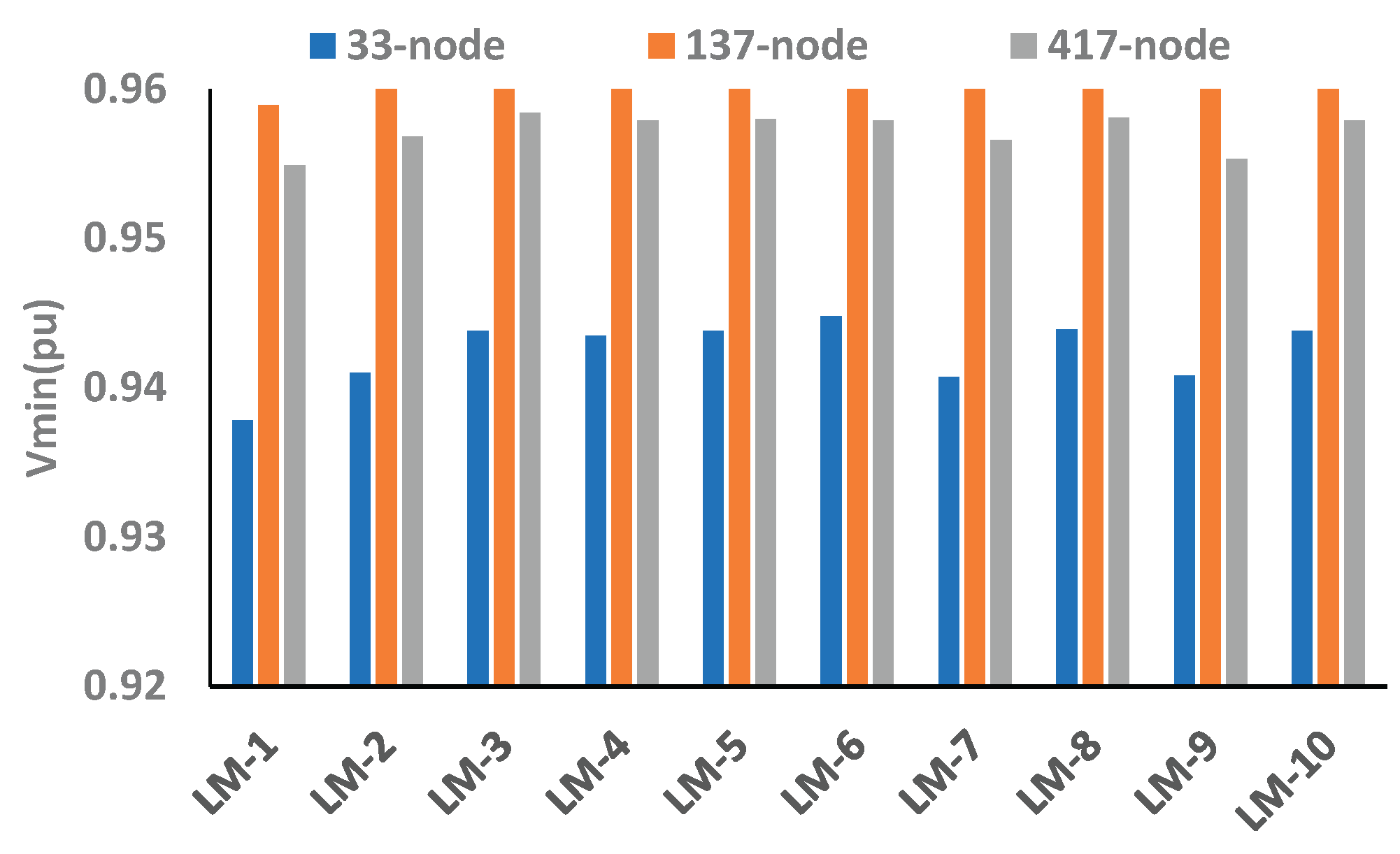
Figure 17.
Objective function under different LMs with no BES.
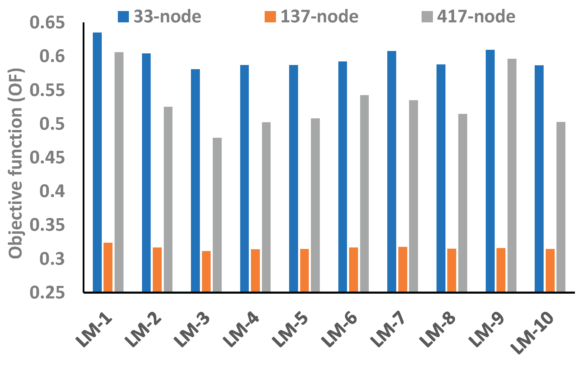
Figure 18.
Voltage profile under different LMs with BES as a load.
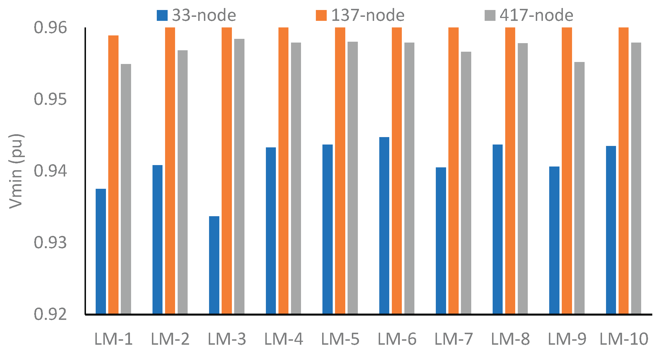
Figure 19.
Objective function under different LMs with BES as a load.
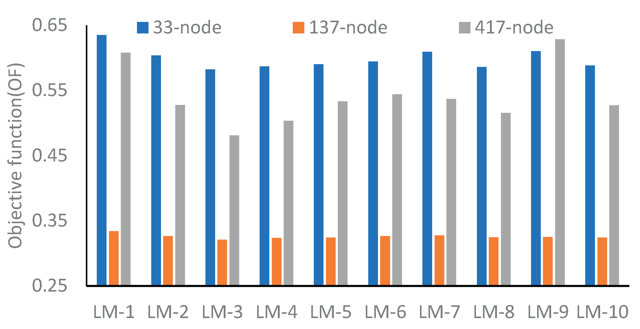
Figure 24.
Voltage profile under different LMs with BES as a source.
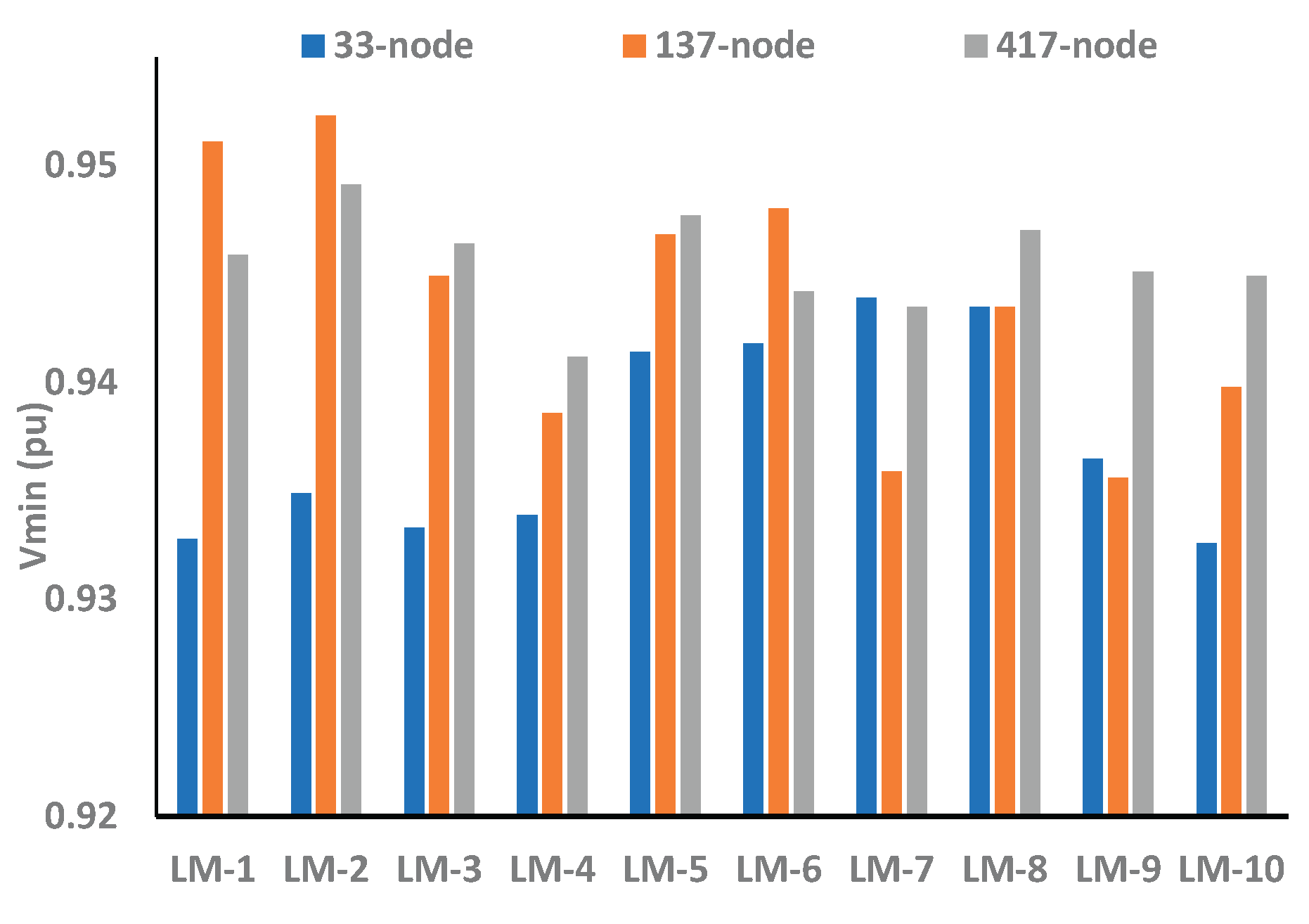
Figure 25.
Objective function under different LMs with BES as a source.
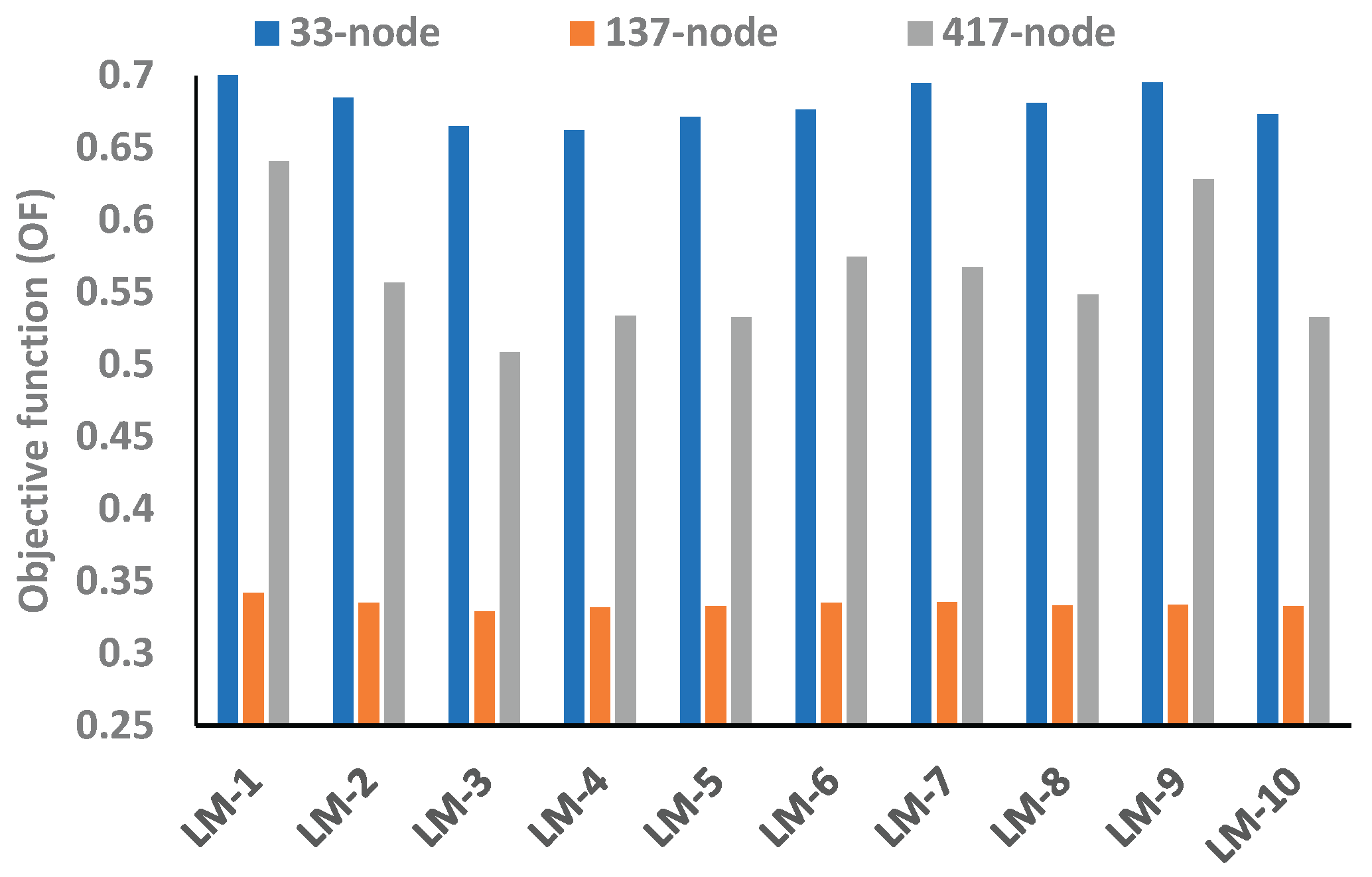
Figure 26.
Variation in objective function in LMs for 33-, 137-, and 417-node RDNs with BES as a load and source.
Figure 26.
Variation in objective function in LMs for 33-, 137-, and 417-node RDNs with BES as a load and source.
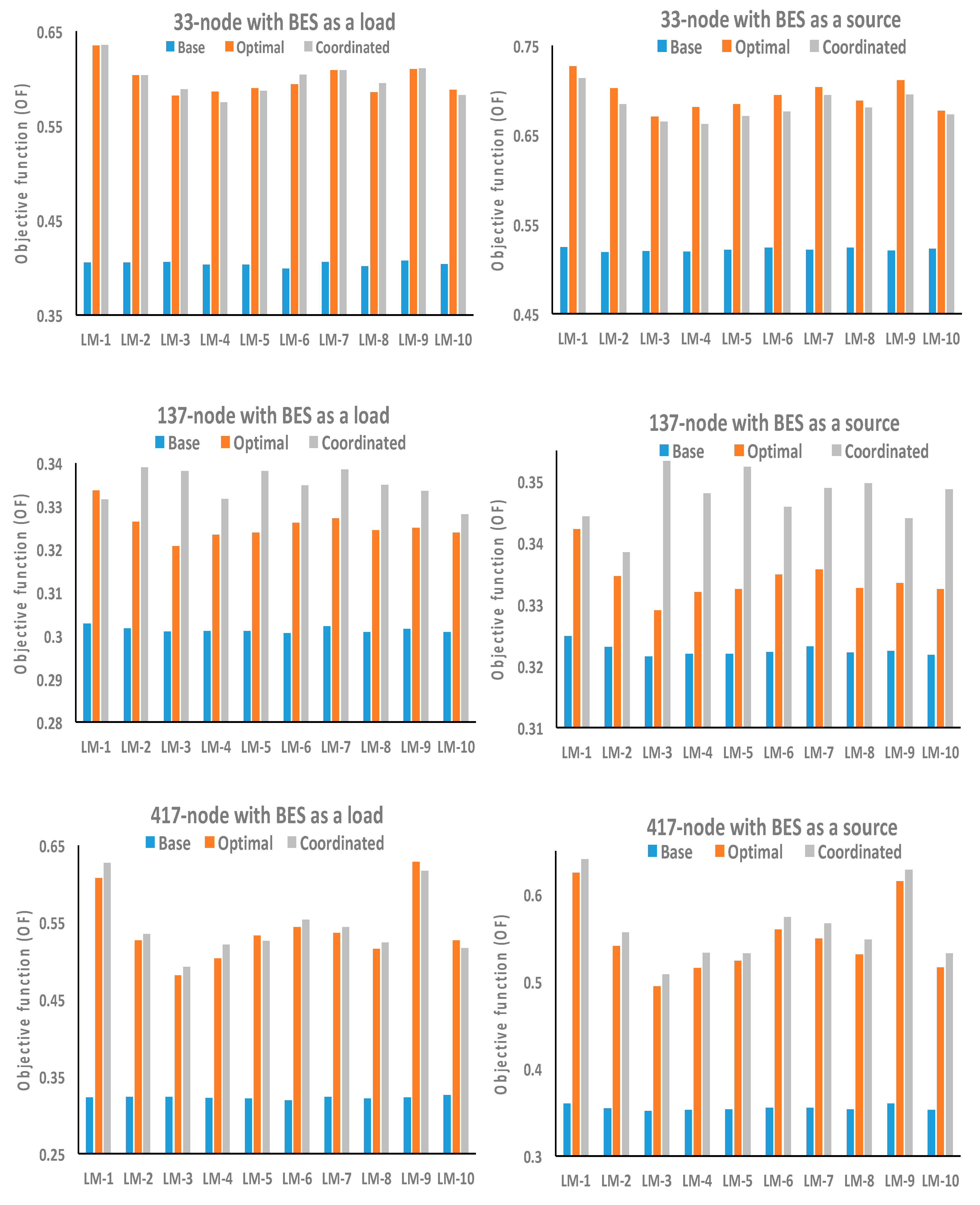
Figure 27.
Convergence characteristics of proposed approach for different RDNs.
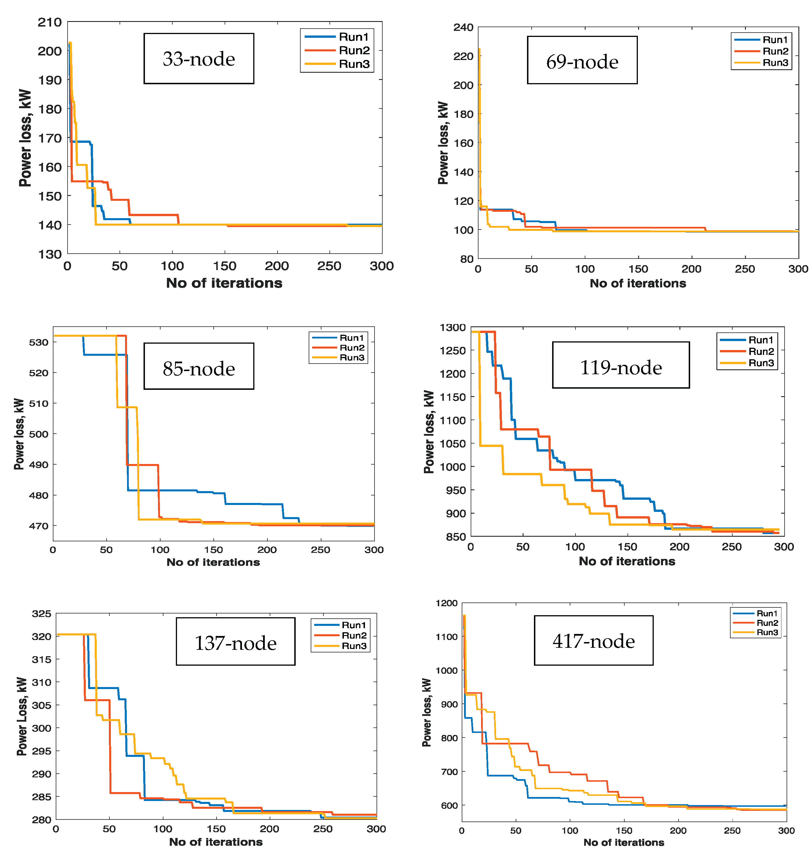
Table 1.
Comparison of different iterative methods for RDNs.
| Methods | LM1 | LM2 | LM3 | LM4 | LM5 | LM6 | LM7 | LM8 | LM9 | LM10 | |
|---|---|---|---|---|---|---|---|---|---|---|---|
| Voltage iterative | CT(sec.) | 0.0120 | 0.0145 | 0.0122 | 0.0133 | 0.0121 | 0.0116 | 0.0143 | 0.0122 | 0.0139 | 0.0122 |
| Count | 3 | 3 | 4 | 4 | 4 | 4 | 3 | 3 | 3 | 4 | |
| Current iterative | CT(sec.) | 0.0121 | 0.0181 | 0.0147 | 0.0140 | 0.0133 | 0.0118 | 0.0193 | 0.0171 | 0.0182 | 0.1340 |
| Count | 4 | 3 | 4 | 4 | 4 | 4 | 3 | 3 | 3 | 4 | |
| Demand iterative | CT(sec.) | 0.0142 | 0.0155 | 0.0120 | 0.0127 | 0.0133 | 0.0121 | 0.0164 | 0.0184 | 0.0178 | 0.0151 |
| Count | 4 | 3 | 4 | 4 | 4 | 4 | 3 | 3 | 3 | 4 | |
Table 2.
Load types and load class with their voltage exponents.
| Load model | Load type | Exponent | Load model | Load class | Exponent | ||
|---|---|---|---|---|---|---|---|
| α | β | α | β | ||||
| LM-1 | Constant power | 0 | 0 | LM-4 | Residential | 1.2 | 2.9 |
| LM-2 | Constant current | 1 | 1 | LM-5 | Commercial | 0.99 | 3.5 |
| LM-3 | Constant impedance | 2 | 2 | LM-6 | Industrial | 0.18 | 6.0 |
Table 3.
EEP analysis of different RDNs in base configuration with no BES.
| Network | Parameters | LM-1 | LM-2 | LM-3 | LM-4 | LM-5 | LM-6 | LM-7 | LM-8 | LM-9 | LM-10 |
|---|---|---|---|---|---|---|---|---|---|---|---|
| 33-node | Vmin(pu) | 0.9131 | 0.9194 | 0.9245 | 0.9229 | 0.9229 | 0.9228 | 0.9187 | 0.9229 | 0.9183 | 0.9229 |
| PLmax(kW) | 51.78 | 45.97 | 41.47 | 42.77 | 42.77 | 43.22 | 46.60 | 42.84 | 47.12 | 42.72 | |
| LImin1 | 3.14 | 3.36 | 3.57 | 3.50 | 3.50 | 3.48 | 3.33 | 3.49 | 3.32 | 3.51 | |
| LImin2 | 13.38 | 14.45 | 15.44 | 15.24 | 15.29 | 15.38 | 14.32 | 15.31 | 14.23 | 15.29 | |
| RImax | 2.0336 | 1.9682 | 1.9129 | 1.9632 | 1.9782 | 2.0376 | 1.9760 | 1.9902 | 1.9635 | 1.9783 | |
| OF | 0.4392 | 0.4379 | 0.4368 | 0.4378 | 0.4382 | 0.4394 | 0.4380 | 0.4384 | 0.4380 | 0.4381 | |
| 137-node | Vmin(pu) | 0.9306 | 0.9351 | 0.9387 | 0.9385 | 0.9388 | 0.9403 | 0.9346 | 0.9391 | 0.9351 | 0.9388 |
| PLmax(kW) | 39.72 | 34.93 | 31.20 | 33.23 | 33.66 | 35.47 | 35.44 | 34.01 | 34.93 | 33.66 | |
| LImin1 | 9.49 | 10.13 | 10.72 | 10.52 | 10.52 | 10.48 | 10.05 | 10.51 | 10.13 | 10.52 | |
| LImin2 | 3.1281 | 3.3213 | 3.5019 | 3.4268 | 3.4208 | 3.4023 | 3.2986 | 3.4155 | 3.3213 | 3.4208 | |
| RImax | 1.6843 | 1.6691 | 1.6545 | 1.6670 | 1.6705 | 1.6836 | 1.6707 | 1.6731 | 1.6945 | 1.6661 | |
| OF | 0.3049 | 0.3037 | 0.3026 | 0.3029 | 0.3028 | 0.3027 | 0.3039 | 0.3028 | 0.3038 | 0.3028 | |
| 417-node | Vmin(pu) | 0.8222 | 0.8479 | 0.8646 | 0.8590 | 0.8585 | 0.8544 | 0.8448 | 0.8576 | 0.8255 | 0.8591 |
| PLmax(kW) | 188.4 | 148.4 | 124.12 | 135.79 | 138.42 | 152.59 | 152.84 | 141.06 | 175.66 | 136.5 | |
| LImin1 | 1.69 | 1.91 | 2.10 | 2.03 | 2.02 | 1.94 | 1.88 | 2.00 | 1.71 | 2.02 | |
| LImin2 | 8.64 | 9.72 | 10.63 | 10.26 | 10.21 | 9.91 | 9.58 | 10.15 | 8.94 | 10.25 | |
| RImax | 6.6003 | 6.1086 | 5.7538 | 6.0277 | 6.1091 | 6.46 | 6.1769 | 6.18 | 6.6527 | 6.0242 | |
| OF | 0.3444 | 0.3414 | 0.3391 | 0.3396 | 0.3395 | 0.3395 | 0.3418 | 0.3396 | 0.3440 | 0.3395 |
Table 4.
EEP analysis of different RDNs in base configuration with BES as a load.
| Network | Parameters | LM-1 | LM-2 | LM-3 | LM-4 | LM-5 | LM-6 | LM-7 | LM-8 | LM-9 | LM-10 |
|---|---|---|---|---|---|---|---|---|---|---|---|
| 33-node | BES-Node | 16,17,17 | 18,17,17 | 7,17,18 | 15,18,18 | 17,16,17 | 18,17,17 | 14,17,18 | 17,18,14 | 14,16,17 | 16,17,16 |
| Vmin(pu) | 0.8998 | 0.9062 | 0.9127 | 0.9104 | 0.9109 | 0.9097 | 0.9062 | 0.9100 | 0.9068 | 0.9114 | |
| PLmax(kW) | 56.65 | 50.13 | 45.09 | 46.67 | 46.74 | 47.52 | 50.83 | 46.87 | 51.38 | 46.66 | |
| LImin1 | 2.72 | 2.93 | 3.06 | 3.11 | 3.00 | 3.01 | 2.95 | 3.09 | 2.89 | 3.03 | |
| LImin2 | 12.56 | 13.58 | 14.54 | 14.31 | 14.34 | 14.38 | 13.46 | 14.35 | 13.37 | 14.35 | |
| RImax | 0.1815 | 0.1773 | 0.1736 | 0.1765 | 0.1773 | 0.1805 | 0.1777 | 0.1779 | 0.1782 | 0.1771 | |
| OF | 0.4060 | 0.4055 | 0.4062 | 0.4036 | 0.4036 | 0.3992 | 0.4062 | 0.4017 | 0.4074 | 0.4040 | |
| 137-node | BES-Node | [119,118 109] | [111,118 119] |
[117,118 119] |
[119,118 111] |
[118,112 119] |
[118,110 119] |
[118,116 109] |
[111,119 117] |
[111,117 119] |
[118,111 119] |
| Vmin(pu) | 0.9263 | 0.9304 | 0.9344 | 0.9341 | 0.9347 | 0.9360 | 0.9312 | 0.9353 | 0.9309 | 0.9344 | |
| PLmax(kW) | 44.41 | 39.09 | 34.96 | 37.27 | 37.75 | 39.85 | 39.66 | 38.17 | 39.09 | 37.76 | |
| LImin1 | 2.94 | 3.12 | 3.35 | 3.21 | 3.22 | 3.19 | 3.09 | 3.27 | 3.18 | 3.21 | |
| LImin2 | 9.05 | 9.65 | 10.22 | 10.03 | 10.2 | 9.98 | 9.58 | 10.02 | 9.65 | 10.02 | |
| RImax | 0.2471 | 0.2424 | 0.2383 | 0.2417 | 0.2427 | 0.2463 | 0.2429 | 0.2434 | 0.2424 | 0.2427 | |
| OF | 0.3029 | 0.3018 | 0.3010 | 0.3011 | 0.3012 | 0.3007 | 0.3022 | 0.3009 | 0.3017 | 0.3009 | |
| 417-node | BES-Node | [38, 43 36] |
[26 42 39] |
[42 32 26] |
[42, 21 39] |
[21 39 42] |
[55 38 33] | [44 53 42] | [26 28 39] | [36 53 44] | [288 42 44] |
| Vmin(pu) | 0.8132 | 0.8402 | 0.8583 | 0.8519 | 0.8512 | 0.8469 | 0.8369 | 0.8507 | 0.8165 | 0.8535 | |
| PLmax(kW) | 198.98 | 155.77 | 129.91 | 142.53 | 145.45 | 161.13 | 160.57 | 148.35 | 185.37 | 141.38 | |
| LImin1 | 1.62 | 1.83 | 2.02 | 1.93 | 1.92 | 1.85 | 1.80 | 1.91 | 1.64 | 1.96 | |
| LImin2 | 8.42 | 9.51 | 10.41 | 10.04 | 9.98 | 9.66 | 9.36 | 9.92 | 8.72 | 10.09 | |
| RImax | 0.2816 | 0.2802 | 0.2788 | 0.2799 | 0.2802 | 0.2814 | 0.2804 | 0.2805 | 0.2802 | 0.2835 | |
| OF | 0.3236 | 0.3239 | 0.3239 | 0.3225 | 0.3219 | 0.3197 | 0.3240 | 0.3217 | 0.3234 | 0.3264 |
Table 5.
EEP analysis of different RDNs in base configuration with BES as a source.
| Network | Parameters | LM-1 | LM-2 | LM-3 | LM-4 | LM-5 | LM-6 | LM-7 | LM-8 | LM-9 | LM-10 |
|---|---|---|---|---|---|---|---|---|---|---|---|
| 33-node | BES-Node | [29 32 31] | [14 16 17] | [18 16 17] | [17 15 16] | [15 17 17] | [15 17 16] | [17 18 16] | [18 16 17] | [18 15 17] | [17 16 18] |
| Vmin(pu) | 0.9159 | 0.9252 | 0.9298 | 0.9290 | 0.9293 | 0.9302 | 0.9246 | 0.9295 | 0.9245 | 0.9293 | |
| PLmax(kW) | 47.46 | 42.20 | 38.16 | 39.21 | 39.16 | 39.34 | 42.76 | 39.18 | 43.21 | 39.13 | |
| LImin1 | 14.24 | 15.38 | 16.42 | 16.24 | 16.30 | 16.47 | 15.24 | 16.33 | 15.15 | 16.30 | |
| LImin2 | 3.23 | 3.57 | 3.79 | 3.77 | 3.79 | 3.86 | 3.55 | 3.80 | 3.55 | 3.79 | |
| RImax | 0.1709 | 0.1667 | 0.1632 | 0.1660 | 0.1668 | 0.1698 | 0.1672 | 0.1674 | 0.1677 | 0.1666 | |
| OF | 0.5249 | 0.5192 | 0.5201 | 0.5196 | 0.5213 | 0.5241 | 0.5218 | 0.5238 | 0.5207 | 0.5228 | |
| 137-node | BES-Node | [114,110, 118] |
[109,113 116] |
[111,116, 113] |
[110,116, 114] |
[108,114 116] |
[114,113 118] |
[114,117 116] |
[116,118 113] |
[111,116 114] |
[112,117 115] |
| Vmin(pu) | 0.9345 | 0.9379 | 0.9417 | 0.9413 | 0.9415 | 0.9436 | 0.9376 | 0.9425 | 0.9382 | 0.9415 | |
| PLmax(kW) | 35.38 | 31.08 | 27.72 | 29.51 | 29.87 | 31.41 | 31.54 | 30.17 | 31.08 | 29.87 | |
| LImin1 | 3.33 | 3.54 | 3.70 | 3.62 | 3.65 | 3.62 | 3.44 | 3.60 | 3.52 | 3.61 | |
| LImin2 | 9.97 | 10.61 | 11.27 | 11.06 | 11.06 | 11.04 | 10.56 | 11.05 | 10.64 | 11.06 | |
| RImax | 0.2265 | 0.2251 | 0.2237 | 0.2248 | 0.2251 | 0.2262 | 0.2252 | 0.2253 | 0.2250 | 0.2251 | |
| OF | 0.3249 | 0.3232 | 0.3216 | 0.3221 | 0.3221 | 0.3223 | 0.3233 | 0.3222 | 0.3225 | 0.3219 | |
| 417-node | BES-Node | [33 30 57] | [42 53 43] | [32 43 33] | [22 36 39] | [47 38 28] | [44 42 52] | [41 48 43] | [53 21 33] | [38 45 26] | [51 38 42] |
| Vmin(pu) | 0.8297 | 0.8549 | 0.8705 | 0.8651 | 0.8647 | 0.8615 | 0.8510 | 0.8641 | 0.8338 | 0.8654 | |
| PLmax(kW) | 178.62 | 141.41 | 118.59 | 129.38 | 131.74 | 144.5 | 145.54 | 134.12 | 166.48 | 130.02 | |
| LImin1 | 1.75 | 1.97 | 2.17 | 2.06 | 2.04 | 1.93 | 1.93 | 2.07 | 1.77 | 2.06 | |
| LImin2 | 8.85 | 9.94 | 10.85 | 10.48 | 10.44 | 10.16 | 9.80 | 10.38 | 9.17 | 10.48 | |
| RImax | 0.2816 | 0.2802 | 0.2788 | 0.2799 | 0.2802 | 0.2814 | 0.2803 | 0.2805 | 0.2802 | 0.2802 | |
| OF | 0.3599 | 0.3552 | 0.3517 | 0.3530 | 0.3535 | 0.3554 | 0.3553 | 0.3539 | 0.3602 | 0.3529 |
Table 6.
EEP analysis of different RDNs in optimal configuration with no BES.
| Network | Parameters | LM-1 | LM-2 | LM-3 | LM-4 | LM-5 | LM-6 | LM-7 | LM-8 | LM-9 | LM-10 |
|---|---|---|---|---|---|---|---|---|---|---|---|
| 33-node | Vmin(pu) | 0.9378 | 0.9410 | 0.9438 | 0.9435 | 0.9438 | 0.9448 | 0.9407 | 0.9439 | 0.9408 | 0.9438 |
| PLmax(kW) | 26.79 | 24.77 | 23.08 | 23.39 | 23.31 | 23.06 | 24.99 | 23.25 | 25.03 | 23.30 | |
| LImin1 | 4.25 | 4.46 | 4.67 | 4.69 | 4.72 | 4.85 | 4.44 | 4.75 | 4.45 | 4.72 | |
| LImin2 | 14.74 | 15.33 | 15.89 | 15.66 | 15.64 | 15.55 | 15.26 | 15.62 | 15.15 | 15.64 | |
| RImax | 1.3902 | 1.3568 | 1.3274 | 1.3412 | 1.3432 | 1.3511 | 1.3606 | 1.3448 | 1.3545 | 1.3432 | |
| OF | 0.6351 | 0.6041 | 0.5809 | 0.5869 | 0.5872 | 0.5925 | 0.6079 | 0.5881 | 0.6096 | 0.5868 | |
| 137-node | Vmin | 0.9589 | 0.9605 | 0.96196 | 0.9619 | 0.9621 | 0.9630 | 0.9603 | 0.9623 | 0.9603 | 0.9621 |
| PLmax | 21.121 | 20.01 | 19.01 | 19.55 | 19.65 | 20.04 | 20.12 | 19.72 | 20.05 | 19.65 | |
| LImin1 | 5.44 | 5.65 | 5.85 | 5.78 | 5.79 | 5.79 | 5.62 | 5.79 | 5.63 | 5.79 | |
| LImin2 | 15.25 | 15.63 | 15.99 | 15.88 | 15.88 | 15.91 | 15.58 | 15.89 | 15.63 | 15.88 | |
| RImax | 1.6733 | 1.659 | 1.6454 | 1.657 | 1.6602 | 1.6724 | 1.6605 | 1.6626 | 1.6819 | 1.6562 | |
| OF | 0.3239 | 0.3169 | 0.3116 | 0.3141 | 0.3146 | 0.3168 | 0.3177 | 0.3150 | 0.3159 | 0.3145 | |
| 417-node | Vmin | 0.9549 | 0.9568 | 0.9584 | 0.9579 | 0.9580 | 0.9579 | 0.9566 | 0.9581 | 0.9553 | 0.9579 |
| PLmax | 57.53 | 53.01 | 49.16 | 51.01 | 51.31 | 52.61 | 53.48 | 51.55 | 56.58 | 51.07 | |
| LImin1 | 5.67 | 5.90 | 6.12 | 6.04 | 6.04 | 6.02 | 5.88 | 6.03 | 5.71 | 6.04 | |
| LImin2 | 14.07 | 14.65 | 15.21 | 14.99 | 14.98 | 14.92 | 14.59 | 14.97 | 14.19 | 14.99 | |
| RImax | 3.2458 | 3.2172 | 3.1891 | 3.2109 | 3.2165 | 3.24 | 3.2202 | 3.2209 | 3.2569 | 3.2102 | |
| OF | 0.6060 | 0.5253 | 0.4794 | 0.5021 | 0.5080 | 0.5425 | 0.5349 | 0.5144 | 0.5963 | 0.5027 |
Table 7.
EEP analysis of different RDNs in optimal configuration with BES as a load.
| Network | Parameters | LM-1 | LM-2 | LM-3 | LM-4 | LM-5 | LM-6 | LM-7 | LM-8 | LM-9 | LM-10 |
|---|---|---|---|---|---|---|---|---|---|---|---|
| 33-node | BES-node | [2 2 3] | [23 2 2] | [2,19, 19] | [3 2 19] | [2, 2, 19] | [19,2, 19] | [2, 19, 19] | [19,3 19] | [2 3 2] | [3 2 2] |
| Vmin(pu) | 0.9375 | 0.9408 | 0.9337 | 0.9433 | 0.9437 | 0.9447 | 0.9405 | 0.9437 | 0.9406 | 0.9435 | |
| PLmax(kW) | 27.88 | 25.51 | 23.07 | 24.11 | 23.30 | 23.05 | 24.98 | 24.12 | 25.92 | 24.02 | |
| LImin1 | 4.22 | 4.45 | 15.89 | 15.66 | 15.64 | 15.54 | 15.25 | 15.62 | 15.15 | 15.64 | |
| LImin2 | 14.73 | 15.33 | 4.66 | 4.67 | 4.72 | 4.84 | 4.43 | 4.72 | 4.43 | 4.71 | |
| RImax | 0.1439 | 0.1415 | 0.1394 | 0.1410 | 0.1415 | 0.1432 | 0.1418 | 0.1418 | 0.1418 | 0.1414 | |
| OF | 0.6349 | 0.6037 | 0.5821 | 0.5865 | 0.5901 | 0.5943 | 0.6090 | 0.5858 | 0.6102 | 0.5882 | |
| 137-node | BES-node | [2,101, 2] |
[2,123 77] |
[65,101 2] |
[87,123 2] |
[101,2 77] |
[87,65 2] |
[101, 123,2] |
[77, 101,2] |
[65,2 101] |
[77,2, 101] |
| Vmin | 0.9589 | 0.9605 | 0.9617 | 0.9619 | 0.9622 | 0.9630 | 0.9604 | 0.9623 | 0.9604 | 0.9621 | |
| PLmax | 21.12 | 20.00 | 19.00 | 19.54 | 19.65 | 20.04 | 20.12 | 19.72 | 20.05 | 19.64 | |
| LImin1 | 5.44 | 5.65 | 5.85 | 5.78 | 5.79 | 5.79 | 5.63 | 5.79 | 5.63 | 5.79 | |
| LImin2 | 15.25 | 15.63 | 15.99 | 15.88 | 15.88 | 15.90 | 15.58 | 15.89 | 15.63 | 15.88 | |
| RImax | 0.2457 | 0.2437 | 0.2418 | 0.2434 | 0.2438 | 0.2454 | 0.2439 | 0.2441 | 0.2442 | 0.2437 | |
| OF | 0.3336 | 0.3264 | 0.3208 | 0.3234 | 0.3239 | 0.3262 | 0.3272 | 0.3244 | 0.3250 | 0.3239 | |
| 417-node | BES-node | [190 2 273] | [363 203,273] | [374, 2 364] | [273 366,352] | [2 191 376] | [351 2 271] | [230 363,124] | [374 275,276] | [124 363,376] | [205 376,380 |
| Vmin | 0.9549 | 0.9568 | 0.9584 | 0.9579 | 0.9580 | 0.9579 | 0.9566 | 0.9578 | 0.9552 | 0.9579 | |
| PLmax | 57.53 | 53.01 | 49.16 | 51.01 | 51.31 | 52.61 | 53.48 | 51.55 | 56.58 | 51.07 | |
| LImin1 | 5.67 | 5.91 | 6.12 | 6.04 | 6.02 | 6.02 | 5.88 | 6.03 | 5.72 | 6.04 | |
| LImin2 | 14.07 | 14.65 | 15.21 | 14.99 | 14.98 | 14.92 | 14.59 | 14.97 | 14.19 | 14.99 | |
| RImax | 0.2816 | 0.2802 | 0.2788 | 0.2799 | 0.2802 | 0.2814 | 0.2803 | 0.2804 | 0.2902 | 0.2802 | |
| OF | 0.6079 | 0.5272 | 0.4811 | 0.5034 | 0.5330 | 0.5439 | 0.5366 | 0.5157 | 0.6281 | 0.5267 |
Table 8.
EEP analysis of different RDNs in optimal configuration with BES as a source.
| Network | Parameters | LM-1 | LM-2 | LM-3 | LM-4 | LM-5 | LM-6 | LM-7 | LM-8 | LM-9 | LM-10 |
|---|---|---|---|---|---|---|---|---|---|---|---|
| 33-node | BES-node | [16 18 15] | [33 17 33] | [16 18 17] | [17 17 18] | [18 17 18] | [11 33 33] | [17 18 18] | [33 33 17] | [33 18 33] | [17 14 17] |
| Vmin(pu) | 0.9379 | 0.9411 | 0.9439 | 0.9436 | 0.9439 | 0.9448 | 0.9408 | 0.9441 | 0.9409 | 0.9439 | |
| PLmax(kW) | 26.78 | 24.77 | 23.08 | 23.39 | 23.30 | 23.06 | 24.98 | 23.24 | 25.02 | 23.30 | |
| LImin1 | 16.69 | 17.34 | 17.97 | 17.73 | 17.71 | 17.65 | 17.27 | 17.70 | 17.15 | 17.72 | |
| LImin2 | 4.25 | 4.47 | 4.67 | 4.69 | 4.73 | 4.86 | 4.45 | 4.75 | 4.45 | 4.73 | |
| RImax | 0.1439 | 0.1415 | 0.1394 | 0.1410 | 0.1415 | 0.1432 | 0.1417 | 0.1418 | 0.1418 | 0.1414 | |
| OF | 0.7274 | 0.7024 | 0.6708 | 0.6816 | 0.6846 | 0.6947 | 0.7037 | 0.6884 | 0.7111 | 0.6771 | |
| 137-node | BES-node | [118,119 111] |
[61,86 111] |
[119 118,63] |
[116,62 118] |
[116,118 111] |
[118,86 62] |
[118,119 116] |
[61,119 116] |
[116,111 118] |
[111,116 118] |
| Vmin | 0.9589 | 0.9605 | 0.9619 | 0.9619 | 0.9622 | 0.9630 | 0.9603 | 0.9623 | 0.9604 | 0.9621 | |
| PLmax | 20.35 | 19.23 | 17.84 | 18.28 | 18.41 | 19.47 | 19.03 | 18.50 | 19.12 | 18.38 | |
| LImin1 | 5.44 | 5.65 | 5.85 | 5.79 | 5.79 | 5.79 | 5.63 | 5.79 | 5.63 | 5.79 | |
| LImin2 | 15.25 | 16.02 | 15.99 | 15.88 | 15.88 | 16.31 | 15.59 | 15.89 | 15.63 | 15.88 | |
| RImax | 0.2457 | 0.2437 | 0.2418 | 0.2434 | 0.2438 | 0.2453 | 0.2439 | 0.2441 | 0.2442 | 0.2437 | |
| OF | 0.3423 | 0.3346 | 0.3291 | 0.3320 | 0.3325 | 0.3349 | 0.3357 | 0.3327 | 0.3335 | 0.3325 | |
| 417-node | BES-node | [26 215 30] | [137 42,215] | [215 28 48] | [28 47 42] | [39 215 33] | [35 215 39] | [48 51 44] | [215 22 42] | [49 25 215] | [48 82 42] |
| Vmin | 0.9549 | 0.9568 | 0.9584 | 0.9579 | 0.9580 | 0.9579 | 0.9566 | 0.9580 | 0.9553 | 0.9579 | |
| PLmax | 57.53 | 53.01 | 49.16 | 51.01 | 51.31 | 52.61 | 53.48 | 51.55 | 56.58 | 51.07 | |
| LImin1 | 5.67 | 5.91 | 6.11 | 6.04 | 6.04 | 6.02 | 5.88 | 6.03 | 5.72 | 6.04 | |
| LImin2 | 14.07 | 14.65 | 15.21 | 14.99 | 14.98 | 14.92 | 14.59 | 14.97 | 14.19 | 14.99 | |
| RImax | 0.2816 | 0.2802 | 0.2788 | 0.2799 | 0.2802 | 0.2814 | 0.2803 | 0.2805 | 0.2802 | 0.2802 | |
| OF | 0.6254 | 0.5415 | 0.4947 | 0.5161 | 0.5240 | 0.5599 | 0.5499 | 0.5312 | 0.6153 | 0.5167 |
Table 9.
EEP analysis of different RDNs in coordination of configuration management and BES as a load.
Table 9.
EEP analysis of different RDNs in coordination of configuration management and BES as a load.
| Network | Parameters | LM-1 | LM-2 | LM-3 | LM-4 | LM-5 | LM-6 | LM-7 | LM-8 | LM-9 | LM-10 |
|---|---|---|---|---|---|---|---|---|---|---|---|
| 33-node | BES-node | [5 7 19] | [19 4 25] | [26 4 19] | [6 18 28] | [19 27 26] | [5 28 2] | [20 19 3] | [2 5 3] | [2 23 19] | [23 3 10] |
| Tieline | 7,14,1017,28 | 7,14,9, 17,28 |
7,14,10, 16,28 |
7,34,11, 15,28 |
7,14,11, 17,28 |
7,14,8, 17,28 |
7,13,9 16,28 |
7,14,11, 17,28 |
7,14,9, 15,28 |
7,14,9, 17,28 |
|
| Vmin(pu) | 0.9322 | 0.9348 | 0.9363 | 0.9320 | 0.9388 | 0.9397 | 0.9325 | 0.9398 | 0.9288 | 0.9387 | |
| PLmax(kW) | 32.29 | 29.88 | 28.25 | 30.12 | 28.06 | 27.64 | 30.35 | 28.02 | 31.27 | 27.71 | |
| LImin1 | 3.97 | 4.12 | 4.25 | 4.02 | 4.39 | 4.47 | 4.02 | 4.41 | 3.84 | 4.39 | |
| LImin2 | 15.44 | 15.92 | 16.77 | 16.19 | 17.14 | 17.35 | 15.80 | 17.18 | 15.48 | 16.96 | |
| RImax | 0.1337 | 0.1323 | 0.1312 | 0.1336 | 0.1322 | 0.1331 | 0.1324 | 0.1324 | 0.1332 | 0.1318 | |
| OF | 0.6357 | 0.6035 | 0.5886 | 0.5749 | 0.5868 | 0.6041 | 0.6089 | 0.5956 | 0.6112 | 0.5827 | |
| 137-node | BES-node | [68 87 80] | [87 100 66] | [133 77 72] | [42 48 4] | [3 48 91] | [102 6 13] | [47 2 123] | [76 104 130] | [130 129 66] | [3 66 65] |
| Vmin(pu) | 0.9480 | 0.9370 | 0.9401 | 0.9459 | 0.9399 | 0.9478 | 0.9445 | 0.9397 | 0.9345 | 0.9543 | |
| PLmax(kW) | 28.20 | 46.18 | 42.94 | 34.41 | 46.31 | 41.57 | 42.56 | 48.60 | 50.89 | 26.84 | |
| LImin1 | 4.35 | 3.88 | 4.04 | 4.32 | 3.98 | 4.45 | 4.16 | 3.95 | 3.60 | 4.81 | |
| LImin2 | 12.72 | 9.16 | 9.52 | 15.09 | 9.30 | 9.98 | 11.99 | 9.12 | 10.94 | 14.56 | |
| RImax | 0.2457 | 0.2437 | 0.2477 | 0.2434 | 0.2438 | 0.2454 | 0.2543 | 0.2483 | 0.2614 | 0.2437 | |
| OF | 0.3316 | 0.3390 | 0.3381 | 0.3317 | 0.3381 | 0.3348 | 0.3385 | 0.3350 | 0.3335 | 0.3281 | |
| 417-node | BES-node | [162 93 65] | [352 375 254] | [60 329 308] | [311 340 90] | [396 249 197] | [349 8 376] | [287 208 303] | [18 298 252] | [406 236 388] | [204 79 323] |
| Vmin(pu) | 0.9460 | 0.9396 | 0.9513 | 0.9459 | 0.9462 | 0.9498 | 0.9404 | 0.9401 | 0.9437 | 0.9493 | |
| PLmax(kW) | 53.99 | 53.28 | 51.12 | 50.56 | 53.57 | 51.95 | 49.03 | 51.03 | 54.12 | 54.80 | |
| LImin1 | 4.86 | 4.38 | 5.28 | 4.85 | 3.46 | 5.17 | 4.43 | 4.39 | 4.68 | 3.48 | |
| LImin2 | 14.52 | 16.18 | 14.91 | 15.26 | 14.67 | 15.19 | 15.54 | 16.65 | 14.58 | 14.48 | |
| RImax | 0.3166 | 0.3117 | 0.3237 | 0.3037 | 0.2802 | 0.2814 | 0.3221 | 0.3220 | 0.3147 | 0.3194 | |
| OF | 0.6269 | 0.5350 | 0.4927 | 0.5213 | 0.5259 | 0.5536 | 0.5440 | 0.5237 | 0.6163 | 0.5167 |
Table 10.
EEP analysis of different RDNs in coordination of configuration management and BES as a source.
Table 10.
EEP analysis of different RDNs in coordination of configuration management and BES as a source.
| Network | Parameters | LM-1 | LM-2 | LM-3 | LM-4 | LM-5 | LM-6 | LM-7 | LM-8 | LM-9 | LM-10 |
|---|---|---|---|---|---|---|---|---|---|---|---|
| 33-node | BES-node | [8 9 16] | [15 17 29] | [14 24 33] | [9 31 11] | [18 17 30] | [15 14 30] | [18 11 16] | [31 16 33] | [29 33 15 | [25 32 17] |
| Tieline | 7,14,9 17,28 |
7,14,9, 31,28 |
7,34,11, 31,28 |
7,14,10, 16,37 |
33,14,10 17,28 |
7,13,10 17,28 |
7,14,9 32,28 |
7,14,10 17,28 |
7,14,9 16,28 |
7,34,10, 31,28 |
|
| Vmin(pu) | 0.9328 | 0.9349 | 0.9333 | 0.9339 | 0.9414 | 0.9418 | 0.9439 | 0.9435 | 0.9365 | 0.9326 | |
| PLmax(kW) | 30.42 | 20.03 | 18.90 | 26.2 | 32.79 | 24.75 | 24.96 | 24.16 | 27.33 | 19.13 | |
| LImin1 | 4.00 | 4.06 | 3.9432 | 4.11 | 4.52 | 4.63 | 4.72 | 4.70 | 4.24 | 3.85 | |
| LImin2 | 15.46 | 13.94 | 14.76 | 20.78 | 17.99 | 17.86 | 17.27 | 18.05 | 16.61 | 14.54 | |
| RImax | 0.1318 | 0.1288 | 0.1626 | 0.1467 | 0.1352 | 0.1300 | 0.1275 | 0.1280 | 0.1292 | 0.1657 | |
| OF | 0.7137 | 0.6844 | 0.6651 | 0.6623 | 0.6710 | 0.6762 | 0.6948 | 0.6808 | 0.6952 | 0.6731 | |
| 137-node | BES-node | [118 97 38] | [107 61 96] | [61 106 28] | [15 39 63] | [36 22 33] | [120 86 49] | [37 26 122] | [35 34 32] | [92 39 37] | [60 31 32] |
| Vmin(pu) | 0.9511 | 0.9523 | 0.9449 | 0.9386 | 0.9468 | 0.9480 | 0.9359 | 0.9435 | 0.9356 | 0.9398 | |
| PLmax(kW) | 26.60 | 24.35 | 35.25 | 47.94 | 36.66 | 42.14 | 47.17 | 40.43 | 48.05 | 46.42 | |
| LImin1 | 4.62 | 4.76 | 4.23 | 3.85 | 4.26 | 4.49 | 3.83 | 4.08 | 3.76 | 3.67 | |
| LImin2 | 14.05 | 14.62 | 12.37 | 9.08 | 12.34 | 9.89 | 9.05 | 9.89 | 8.94 | 9.22 | |
| RImax | 0.2457 | 0.2437 | 0.2418 | 0.2434 | 0.2438 | 0.2454 | 0.2439 | 0.2441 | 0.2442 | 0.2437 | |
| OF | 0.3443 | 0.3385 | 0.3533 | 0.3481 | 0.3524 | 0.3459 | 0.3489 | 0.3497 | 0.3440 | 0.3487 | |
| 417-node | BES-node | [29 213 245] | [87 158 132] | [185 32 187] | [215 412 402] | [112 392 81] | [75 27 168] | [168 355 8] | [77 12 156] | [55 56 31] | [36 59 131] |
| Vmin(pu) | 0.9459 | 0.9491 | 0.9464 | 0.9412 | 0.9477 | 0.9442 | 0.9435 | 0.9470 | 0.9451 | 0.9449 | |
| PLmax(kW) | 54.85 | 53.01 | 46.60 | 47.06 | 52.40 | 49.15 | 50.09 | 50.46 | 55.34 | 48.13 | |
| LImin1 | 4.86 | 5.15 | 4.91 | 4.48 | 4.99 | 4.69 | 4.66 | 4.94 | 4.79 | 4.76 | |
| LImin2 | 15.08 | 14.65 | 16.29 | 15.94 | 14.82 | 15.98 | 15.38 | 16.22 | 15.19 | 15.44 | |
| RImax | 0.2817 | 0.3040 | 0.3129 | 0.3143 | 0.2892 | 0.3162 | 0.3176 | 0.3087 | 0.3084 | 0.3147 | |
| OF | 0.6406 | 0.5566 | 0.5083 | 0.5336 | 0.5329 | 0.5745 | 0.5671 | 0.5485 | 0.6281 | 0.5327 |
Table 11.
Computational performance of proposed approach for 33-, 137- and 417-node RDS with PINV.
| Network | 33-node RDN | 137-node RDN | 417-node RDN | ||||||
|---|---|---|---|---|---|---|---|---|---|
| PINV | Max PL | Min PL | CT | Max PL | Min PL | CT | Max PL | Min PL | CT |
| 0.0 | 160.66 | 139.97 | 0.14 | 320.36 | 285.61 | 1.54 | 853.68 | 667.74 | 20.85 |
| 0.1 | 163.82 | 139.55 | 0.56 | 303.29 | 281.73 | 8.24 | 631.70 | 586.58 | 30.27 |
| 0.2 | 144.73 | 139.55 | 0.95 | 286.42 | 280.36 | 6.95 | 656.56 | 590.04 | 52.68 |
| 0.3 | 144.57 | 139.55 | 0.68 | 286.24 | 280.40 | 7.32 | 618.25 | 583.38 | 39.46 |
| 0.4 | 143.71 | 139.55 | 0.84 | 285.51 | 280.30 | 6.56 | 625.38 | 586.94 | 56.31 |
| 0.5 | 143.93 | 139.55 | 0.79 | 284.82 | 280.30 | 6.60 | 666.29 | 587.86 | 84.44 |
| 0.6 | 143.71 | 139.55 | 0.79 | 284.48 | 280.22 | 6.24 | 609.88 | 584.40 | 55.79 |
| 0.7 | 143.71 | 139.55 | 0.74 | 284.85 | 280.19 | 5.72 | 600.36 | 584.17 | 40.87 |
| 0.8 | 143.71 | 139.55 | 0.72 | 284.02 | 280.19 | 6.92 | 593.95 | 582.32 | 22.39 |
| 0.9 | 143.93 | 139.55 | 0.97 | 284.60 | 280.33 | 6.38 | 606.88 | 587.77 | 56.12 |
| 1.0 | 144.52 | 139.55 | 1.03 | 283.74 | 280.75 | 6.82 | 605.00 | 587.69 | 75.01 |
Table 12.
Computational performance of proposed approach for 33-, 69, 85-, 119-, 137- and 417-node RDS with PINV=0.8.
Table 12.
Computational performance of proposed approach for 33-, 69, 85-, 119-, 137- and 417-node RDS with PINV=0.8.
| Network | Tie-lines of minimum loss configuration (optimal) |
PL, kW | CT (sec) | |||
|---|---|---|---|---|---|---|
| Proposed | [16] | [28] | [29] | |||
| 33-node | 7, 9, 14, 32, 37 | 139.55 | 0.7921 | 1.39 | 1.92 | 0.46 |
| 69-node | 14, 58, 61, 69, 70 | 98.60 | 2.4094 | 5.30 | -- | 2.42 |
| 85-node | 8, 14, 35, 40, 43, 56, 63, 73, 84, 87, 90, 91, 93 | 469.89 | 3.4999 | 7.75 | 3.69 | 2.58 |
| 119-node | 24, 26, 35, 40, 43, 51, 59, 72, 75, 96, 98, 110, 122, 130, 131 | 853.59 | 6.6511 | 8.23 | 83.4 | 10.73 |
| 137-node | 8, 36, 52, 91, 97, 107, 119, 127, 136, 138, 139, 142, 143, 145, 146, 147, 148, 149, 151, 152, 156 | 280.19 | 6.2435 | -- | 20.44 | 7.07 |
| 417-node | 7, 15, 17, 18, 22, 27, 32, 55, 56, 61, 70, 74, 87, 88, 95, 97, 98, 112, 116, 129, 143, 146, 151, 156, 157, 159, 164, 169, 170, 179, 180, 196, 200, 214, 215, 253, 255, 267, 283, 302, 322, 323, 359, 363, 370, 393, 396, 397, 401, 403, 404, 417, 424, 432, 437, 438, 447, 450, 467 | 582.32 | 25.0918 | -- | -- | 9942.87 |
Disclaimer/Publisher’s Note: The statements, opinions and data contained in all publications are solely those of the individual author(s) and contributor(s) and not of MDPI and/or the editor(s). MDPI and/or the editor(s) disclaim responsibility for any injury to people or property resulting from any ideas, methods, instructions or products referred to in the content. |
© 2025 by the authors. Licensee MDPI, Basel, Switzerland. This article is an open access article distributed under the terms and conditions of the Creative Commons Attribution (CC BY) license (https://creativecommons.org/licenses/by/4.0/).
Copyright: This open access article is published under a Creative Commons CC BY 4.0 license, which permit the free download, distribution, and reuse, provided that the author and preprint are cited in any reuse.


