Submitted:
17 September 2025
Posted:
18 September 2025
You are already at the latest version
Abstract
Currently, the demand for electrical energy is increasing significantly due to population growth, rapid industrialization, and automation. Distribution systems with long power supply distances and weak network structures, in particular, greatly benefit from the integration of renewable energy sources (RES). The integration of wind turbines (WT), photovoltaic systems (PV), and distribution static synchronous compensator (D-STATCOM) controllers in power systems is crucial for enhancing voltage profiles, minimizing power losses, and improving the reliability of radial distribution networks (RDS). This study presents an innovative approach for the optimal allocation and sizing of WT, PV, and D-STATCOM within RDS, aiming to significantly enhance voltage pro-files and reduce both active and reactive power losses. A hybrid HGA-PSO algorithm, a powerful and efficient metaheuristic technique, is utilized to determine the optimal allocation and sizing of WT, PV, and D-STATCOM controllers. The loss sensitivity factor (LSF) technique is employed to prioritize buses for optimal placement, while the voltage stability index (VSI) identifies buses susceptible to voltage collapse, ensuring strategic integration of WT, PV, and D-STATCOM. To validate the effectiveness of the HGA-PSO-based approach, simulations are conducted on a 139-bus RDS. The results indicate that the strategic placement of WT, PV, and D-STATCOM significantly en-hances the voltage profile across the distribution network, leading to improved power quality and reduced power losses. Simulations on the 139-bus system with WT and solar PV demonstrate a 43.69% reduction in active power losses, while reactive power losses improve by 58.32% compared to the base case scenario.
Keywords:
renewable energy sources (RES)
; radial distribution networks (RDS)
; voltage resilience
; power losses
; hybrid genetic algorithm
1. Introduction
Currently, the demand for electrical energy is significantly increasing as a result of the growing population, the fast industrialization process, and its automation. However, traditional investments in transmission and distribution infrastructure and the usage of fossil fuels are gradually declining [1]. This encourages the power supply companies to confront unprecedented challenges in meeting load requirements, ensuring customer satisfaction, and addressing environmental constraints. Due to variations in radial topologies and voltage levels, distribution systems have higher losses than transmission networks [2]. In particular, distribution systems with a long power supply distance and a weak network structure benefit greatly from the integration of renewable energy sources (RES). These benefits include shifting peak loads, lowering network losses, increasing system reliability, and improving voltage profiles [3].
However, the integration of RES into modern power grids presents challenges like voltage instability, power quality issues, and network losses. Since solar and wind energy rely on weather conditions, power generation can fluctuate unpredictably, making voltage stability harder to maintain. Unlike centralized power generation, renewables are often distributed across the grid, sometimes causing localized voltage rises or drops [3,4,5]
From the perspective of RES design, most research studies consider non-dispatchable energy sources, such as photovoltaic (PV) and wind turbines (WTs), whose electricity generation cannot be easily adjusted to meet real-time electricity demand due to their dependence on environmental conditions. This reliance causes variations in voltage profiles and increases power losses, which can negatively impact power quality [6,7,8,9]. The unpredictability of non-dispatchable energy sources' outputs affecting power quality is analyzed using artificial intelligence and stochastic theory [10]. Traditionally, reactive power has been controlled with fixed capacitor banks and synchronous condensers, but these methods have several drawbacks, such as inefficiency, slow response, high cost, and the potential to cause overvoltage or harmonic issues [11,12]. To address these concerns, custom power devices, particularly the distribution static synchronous compensator(D-STATCOM), have been introduced. D-STATCOM efficiently mitigates power quality challenges by compensating for reactive power, thereby reducing power losses and voltage fluctuations [13,14]. Additionally, determining the optimal placement and size of WT and PV systems within radial distribution systems (RDS) is essential for minimizing power losses and improving voltage profiles [15,16]. Intelligent search methods are widely used for solving complex optimization problems, offering efficiency but often leading to locally optimal solutions rather than global ones [17]. Various techniques, including genetic algorithm (GA), particle swarm optimization (PSO), GA-PSO hybrid algorithm, honey bee mating optimization (HBMO), and ant colony optimization (ACO), have been applied to overcome these challenges [18]. Additionally, differential evolution (DE) and artificial neural networks (ANNs) are gaining prominence for their ability to enhance optimization performance and improve solution accuracy in complex systems [19].
This study employs the HGA-PSO algorithm, integrating the voltage stability index (VSI) and loss sensitivity factor (LSF) to determine the optimal location and sizing of WT, PV, D-STATCOM, and their combinations within the power distribution grid. VSI is used to identify the best placement and prioritization for WT, PV, PV-WT, and PV-WT-DSTATCOM, while LSF is used to determine the optimal size for each.
2. Materials and Methods
Power flow analysis examines the current and voltage at each bus, along with the active and reactive power flows in each line [20]. While conventional algorithms are essential for transmission networks, they are less effective for radial distribution systems (RDS) due to their low reactance to resistance (X/R) ratios. As a result, traditional methods such as Gauss Seidel and Newton Raphson are not well-suited for RDS analysis [21,22].
To analyze the total electrical power loss in a power grid with integrated PV systems and WT, the following mathematical framework is utilized. At each bus, net active and reactive power injection is formulated as:
Where , is time dependent active power from PV and WT while , is time dependent reactive power contributions from inverters in providing voltage support.
The Jacobian matrix gives the linearized relationship between small changes in voltage angle and voltage magnitude with small changes in real and reactive power [24].
Elements of Jacobian matrix are the partial derivatives evaluated at and . It can be written as:
2.1. System Configuration
The PV and WT systems are integrated with the main power grid to generate electricity under normal operating conditions and in grid-connected mode. However, since solar radiation and wind speed fluctuate seasonally and can be unpredictable, energy production is not always consistent [7]. To mitigate this, a storage system is incorporated to store excess energy produced during high-generation periods and supply electricity when renewable generation is low. This ensures a stable and reliable power supply for local loads, reducing dependence on external sources. The schematic configuration for this study is illustrated in Figure 1.
2.2. Modeling of System Components
1) Modelling of DSTATCOM
D-STATCOM is a shunt device that regulates bus voltage and power factor by injecting or absorbing real and reactive power. It operates as a voltage-source inverter with a DC energy storage unit or capacitor to ensure stable DC voltage. Acting as a synchronous voltage source, it eliminates voltage sag/swell and maintains system stability [25]. The expression for reactive power injection is:
Where is voltage at the point of common coupling, is output voltage of the DSTATCOM, is phase angle difference, is coupling reactance. The controller adjusts to maintain at the reference voltage , expressed as:
2) Modelling of Solar Panel Array
Solar energy shows great potential as a renewable source for sustainable electricity generation, with extensive studies evaluating its efficiency and power output [26]. PV panel efficiency is affected by various factors, including placement, shading, maintenance, dust buildup, solar exposure, climate conditions, installation techniques, and module selection [27]. PV cells are connected in series to regulate voltage and in parallel to enhance current capacity. Together, they form a module whose overall power output is determined by the product of voltage and current [28]. The performance of a PV system is evaluated based on its rated power, actual solar irradiance, and ambient temperature.
Where , is the output power of the solar panel array in Watts (W), is the nominal power of the solar PV panel, is the derating factor relative to the losses due to accumulation of dust on the panels and the ambient temperature effect, is the incident solar radiation on the tilted surface of the solar PV panels in , is the incident solar radiation on the cell surface under standard conditions, typically 1000 , is the temperature coefficient of the PV module, typically around for the mono and polycrystalline (Si) solar cells[29], is the standard test condition temperature, usually 25 , is the cell temperature under operating conditions and is given by:
Where, is the ambient temperature.
The clearness index is a dimensionless quantity that measure the transparency of the atmosphere by comparing the solar radiation received at the Earth's surface to the extraterrestrial radiation at the top of the atmosphere and is defined as the surface radiation divided by the extraterrestrial radiation.
3) Modelling of Wind Turbines
WT power is influenced by wind speed, and effective placement is crucial to avoid disruptions. Betz’s law states that a turbine can capture 59.3% of kinetic energy, ensuring maximum wind power extraction efficiency [30]. Electricity generation begins at the cut-in wind speed, when the turbine starts operating. The power output is influenced by wind density, blade-swept area, and efficiency coefficient. As wind speed increases, turbines reach their maximum power at the rated speed, shutting down if it exceeds the cut-out speed, which is expressed as:
Where, is the reference wind speed measured at the reference hub height , is the wind speed measured at the hub height ,and is the power law exponent. It is affected by several factors, including wind speed, terrain roughness, height above ground, temperature, and the time of day. It is in range of 0.10 to 0.25. Typically, 0.11 is used for extreme wind conditions, while 0.2 is considered standard for normal conditions. However, a value of 1/7 is frequently used in practice. The rated power of the wind turbine is determined by [31]:
Where is air density at standard conditions, is the effective area of the rotor, is coefficient of performance of turbine efficiency, up to 0.59 due to the Betz limit, and is generator mechanical efficiency, up to 0.95 accounts for losses in conversion to electrical energy.
The output power of the wind turbine generator is determined by using equation (14). The cut-in ratio (CIR) is used to determine the output of the wind turbine. CIR is a dimensionless parameter that defines the ratio of the cut-in wind speed to the rated wind speed, expressed as:
4) Modelling of Energy Storage Unit
An energy storage unit, such as batteries, plays a crucial role in integrated energy systems, ensuring reliability and an uninterrupted power supply during energy shortages [32]. The Battery Bank capacity can be determined using the following formula:
Where Load (W) is the total power consumption of all connected devices in watts, Backup Time (h) is the desired duration (in hours) the battery must sustain the load demand before complete depletion, Voltage (V) is the nominal voltage of the battery bank, and Depth of Discharge (DoD) is the fraction of the battery capacity that can be safely used, and , represent the efficiencies of the inverter and the battery, respectively.
Properly sizing a battery bank in a hybrid renewable energy system requires considering autonomy days to prevent power shortages and store surplus energy for future use. The power interaction within the battery bank in such a system can be expressed as follows:
Where is total renewable generation and is adjusted load demand. The state of charge (SOC) is a crucial indicator of a battery bank’s operational condition, indicating the remaining capacity relative to its total capacity. The SOC is determined by examining both its charging and discharging cycles. Therefore,
Surplus Scenario:
Deficit Scenario:
2.3. Real Power Loss Formulation
The branch current method is widely applied in radial distribution networks integrated with PV and WT due to its compatibility and computational efficiency [33]. By considering WT, PV and D-STATCOM in the system, the power losses under the constraints can be computed as follows [34]. The total real power loss in a power distribution system with WT, PV integration can be formulated as:
Where is resistance of branch , , are real and reactive power flows in branch ,which depend on load demands at downstream nodes, power injections from PV, WT, and voltage profile at the sending-end node of branch . Similarly, total reactive power loss can be formulated as:
Considering RES penetration, the real and reactive power contributions from WT, PV at bus are represented by and , respectively. Consequently, the net power flow in branch is expressed as:
WT, PV reduces the net power drawn from the power grid, altering and , thereby affecting losses. Losses are inversely proportional to , emphasizing the role of D-STATCOM voltage regulation devices in loss minimization. For optimal allocation/sizing of WT, PV and D-STATCOM, the loss equation is linearized or approximated using sensitivity factors:
Here, represents the nominal voltage, typically set to 1 p.u., while and are dependent on the locations and capacities of the WT,PV and DSTATCOM. The percentage reduction in active and reactive power losses due to the integration of WT, PV and DSTATCOM is computed as follows:
Where, and are total active and reactive power losses without integration, and are total active and reactive power losses with integration.
2.4. Dynamic Voltage Resilience Margin Deviation (DVRMD)
Intermittent RES causes voltage fluctuations, but grid stability remains despite challenges like load changes. Deviations from a ±5% stability threshold can cause blackouts, and lower dynamic voltage resilience margin deviations enhance system voltage profile [34]. It is formulated as:
Where is the total number of buses, is the voltage magnitude at bus , is the reference voltage which is 1.0 p.u. Net voltage at bus is expressed by:
Where represents the voltage adjustment at bus caused by WT,PV, which is calculated based on the active and reactive power injections and and the grid impedance. It is expressed by:
2.5. Voltage Stability Index (VSI)
The Voltage Stability Index (VSI) is a crucial metric used to identify buses susceptible to voltage collapse in renewable integrated power grid systems. It accounts for line parameters, bus power injections, and voltages. A low VSI bus value increases the likelihood of locating renewable energy sources. For a distribution line between buses (sending) and (receiving), a common VSI formulation is expressed as:
Where is the sending bus voltage, while , , , are real power, reactive power, resistance, and reactance for the receiving bus, respectively.
2.6. Loss Sensitivity Factor (LSF)
LSF is a crucial metric for determining the optimal placement of WT, PV, and DSTATCOMs, helping identify buses where reactive power compensation minimizes active power losses. LSF prioritizes buses where WT, PV and DSTATCOM placement will most effectively reduce losses under variable load conditions. LSF indirectly supports voltage stability by reducing line loading and improving reactive power balance. The LSF for bus is obtained by taking the derivative of the total system losses with respect to the reactive power injected at that specific bus.
For a distribution line between buses and , the LSF can be approximated as:
Where , are active and reactive power at bus , , is resistance and reactance of the line between buses and , is voltage magnitude at bus .
4. Objectives and System Constraints
4.1. Objective Function
To address the optimal allocation and sizing of WT, PV, and DSTATCOM in power grids using a HGA-PSO algorithms, the following objective functions and system constraints are formulated to achieve dynamic loss minimization and voltage resilience:
- 1) Dynamic Active Power Loss Minimization
Where
and
are real/reactive power flow in branch
at time
.
is voltage magnitude at branch
. The purpose is to minimize time-aggregated resistive losses across all branches, accounting for RES variability and load fluctuations over
time intervals.
- 2) Dynamic Reactive Power Loss Minimization
- 3) Voltage Resilience Enhancement
Where
is net voltage magnitude at bus
at time
.
is the reference voltage which is 1.0 p.u. The purpose is to minimize voltage deviations across all buses to ensure stability under dynamic RES penetration.
- 4)
- Total Cost Minimization
- 5)
- Multi-Objective Formulation
Where , , and are the weighting factors related to active power loss, reactive power loss voltage deviation and total cost minimization over time intervals, respectively. The weighting factors are formulated to provide an impact index associated with the connection of WT, PV and D-STATCOM. It prioritizes loss reduction while ensuring voltage compliance.
4.2. System Constraints
4.2.1. Equality Constraints
The equality constraints for the optimal allocation and sizing of WT, PV and DSTATCOM-integrated power grid are fundamental equations that ensure physical and operational laws are satisfied.
- Real power balance at each bus
Where is the power supplied by the utility grid ,is the power supplied by WT, and PV, is the load demand, is total active power loss, is the number of WT, is the number of branches in the distribution network.
4.2.2. Inequality Constraints
- B.
- Voltage Limit Constraint
The system's voltage magnitude must remain within the specified minimum and maximum limits to prevent reverse power flow and mitigate an increase in inrush current.
Where
and
are the minimum and maximum permissible voltage at bus
, respectively.
- C.
- Active power limit constraints
The total capacity of all WT, PV should not exceed the load demand, with integration limited to 60% of the feeder's real power demand and a minimum capacity of zero [35].
Where and represent the real power injected by the WT, PV and the active load demand, respectively.
- D.
- Reactive Power Limits constraint
Where and denote the minimum and maximum reactive power demand compensated at bus , respectively.
- E.
- Design Variables constraints
The study explores the influence of PV module quantity, WT capacity, and battery system deployment on overall performance and identifies necessary constraints for optimal system configuration.
The battery storage system (BSS) maintains its state of charge (SOC) within predefined minimum and maximum limits to ensure stable operation.
4.3. HGA-PSO Algorithms
The research provides a detailed algorithmic explanation for optimizing the location and sizing of WTs, PVs, and D-STATCOMs using the HGA-PSO process, which involves a three-step process [36]. Assume that is a population of individuals at generation :
Where,
The function value of each individual is evaluated from the objective function.
Step 1: The global best, the local best and worst are identified from the population:
The variable represents the current generation. In the current population, and denote the local best and worst function values, respectively, while and represent the global best position and its corresponding function value, which reflect the optimal value discovered in the population so far. The values obtained from equation 48c are utilized to direct the movement of all individuals toward the global solution.
Step 2: Each individual is updated based on the global best, local worst, and its own function value. The following formula calculates a new value for the individual.
Where, is the ratio of the difference between and to that between and , and is a positive constant that was empirically selected to guarantee a notable improvement in the HGA's performance. has a value that ranges from 0 to 1, inclusive. A Gaussian distribution, ,with mean and standard deviation , is used to sample . As a result, each individual is given a value that is probably close to ,with some variation.
Step 3: Equation 4.17, the HGA involves random mutations affecting selected genes or variables, enhancing genetic diversity and preventing premature convergence to local optima.
The mutation process involves selecting a gene , altering it to ,based on uniform random number , and the shape decay rate parameter . The mutation rate controls the balance between conservative and exploratory search strategies, while shapes the mutation distribution, with higher narrowing and lower broadening the distribution.
The Particle Swarm Optimization (PSO) algorithm refines candidate solutions by utilizing individual and collective experiences of particles, which dynamically adjust their positions to improve the likelihood of reaching an optimal solution[34]. The optimization of the candidate solution, ,is achieved through the iterative adjustment of particle velocities and positions, guided by specific update equations for each particle. Proper weight choice offers a good balance between global and local exploration.
Velocity Update is given by:
Where, is the velocity of particle at iteration, is the particle's inertia weight, is the velocity of particle at iteration , , are positive constants restricted to values within , , are numbers randomly generated within , is the optimal position of the particle determined through its individual experience, is the optimal global position of the particle within the population, is the position of the particle at the iteration.
Position Update is given by:
Where is constriction factor. It helps to ensure convergence.
4.3. Site Description and System Specifications
4.3.1. Geographical Location and Climatic Conditions
The proposed system, a WT and PV integrated power distribution network, is located in Adama City, approximately 8.54°N latitude and 39.27°E longitude[36], in the Oromia region of Ethiopia, about 99 km southeast of Addis Ababa[37].
Adama has a semi-arid climate, characterized by distinct wet and dry seasons. Ambient temperature typically ranges from 15°C to 30°C, with warm days and cooler nights. Adama, a region with abundant sunshine, is ideal for solar and wind power generation due to its favorable climate and rainfall patterns. Meteorological data on wind speed, solar radiation, and ambient temperature for the simulations were obtained from NASA at the coordinates of Adama City (8.54°N, 39.27°E) for the specified year. The monthly average wind speed, solar radiation, and ambient temperature were 3.28 m/s ,0.275683 kW/m², and 293.4 K, respectively.
4.3.2. Load Characteristics
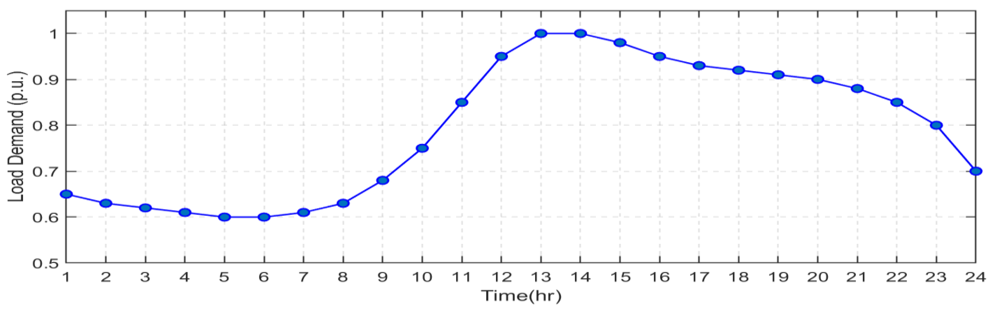
This research employed direct load estimation methodologies to assess loads in renewable energy system-integrated grids, ensuring precise power consumption calculations within distribution networks. The evaluated power distribution network is assumed to follow the standardized 24-hour load profile of the IEEE system, as depicted in Figure 5[38]. Active power (P) and reactive power (Q) are incorporated into the analysis using the load factor (LF) as defined in the formula below.
Where, LF is the load factor quantifies how efficiently energy infrastructure is utilized and t is time in hours.
Figure 5.
Daily load profile curve.
4.5. PV and WT-Integrated Grid Energy Generation System
This study analyzes WT and PV distributed generation units, which generate energy based on normalized average output curves. These curves show hourly energy production relative to the daily peak output. The capacity factor (CF) is calculated as the ratio of the area under the normalized output curve to the total time period[39].
Figure 6.
Daily WT and PV Energy output curves.
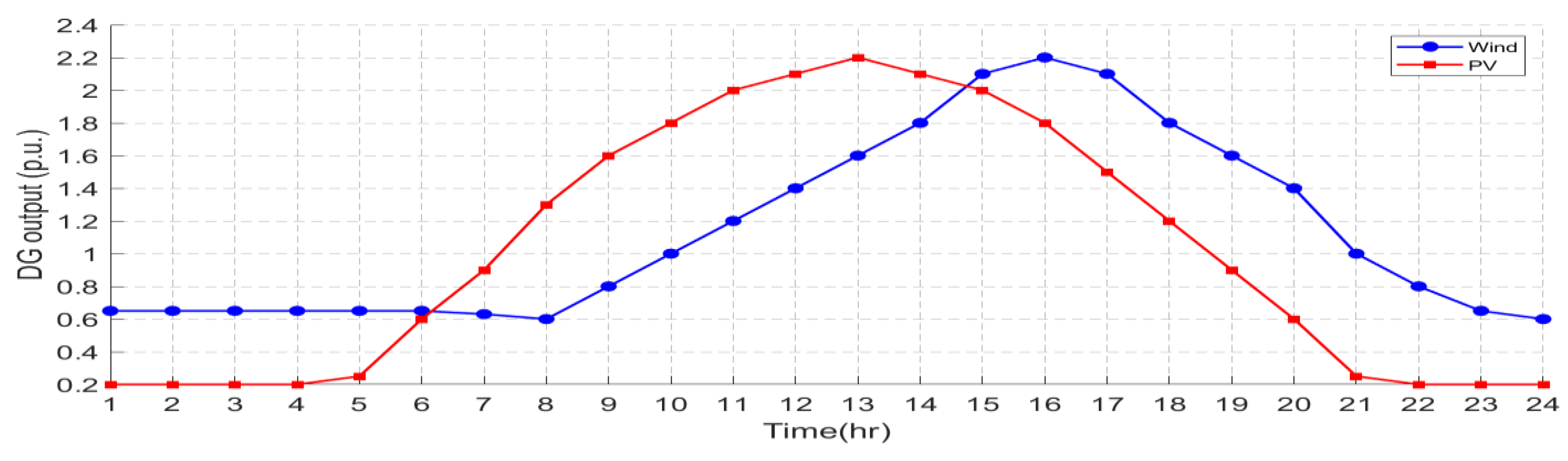
Figure 7 and Figure 8 illustrate the contribution of power generation and investment cost percentages for RES components within the grid, respectively. PV panels contribute 62% of the total power output, with an associated investment cost of 40%. Wind turbines (WT) generate nearly 40% of the power while requiring a 35% investment cost. Battery energy storage provides 18% of the power, with an associated investment cost of 15%.
5. Simulation Results and Discussions
The simulation results provide a comparative analysis of the base case with the integration of WT, PV, PV-WT, and PV-WT-D-STATCOM in the 139-bus system. This section presents the outcomes obtained through the NR load flow method and the combined HGA-PSO algorithm. The load flow analysis was conducted using the NR algorithm in MATLAB 2024a, utilizing line and bus data. All values were normalized to per-unit (p.u.) based on a 100 MVA system base and a 15-kV base voltage to ensure consistency. Voltage limits were maintained between 0.95 and 1.05 p.u. to ensure system stability.
The impact of weight factors on fitness values, HGA-PSO input parameters, and optimization process boundary conditions is outlined in Table 1. The selection of appropriate weight factors is vital for achieving optimal results. These factors are determined based on engineering priorities, with a strong focus on minimizing real power losses and improving dynamic voltage resilience margin deviation due to their significant influence on reducing overall costs. While other aspects remain important, the assigned weights reflect these priorities.
To identify the optimal combination of weight factors, Multi-Objective Function (MoF) simulations were conducted using MATLAB Software. The selected weights aimed to minimize the objective function value while maintaining a balance between competing objectives. In this study, the best results were achieved using different combination of weight factors. Prioritizing a high weight for and low weights for effectively minimizes the function value, achieving the best outcome with a value of 0.02268. In contrast, distributing weights evenly across results in poor performance, with the worst outcome being a function value of 0.039631. This demonstrates the importance of strategic weight allocation in optimization, as detailed in Table 2.

Table 1.
proposed HGA-PSO parameters.
| HGA Parameters | Size of populations | 30 | ||
| A Gaussian distribution | [1.8,0.01] | |||
| Mutation rate | 0.05 | |||
| Shape parameter | 6 | |||
| PSO Parameters | Size of the swarm (population). | 30 | ||
| The particle's weight due to inertia | 0.4 | |||
| Cognitive Coefficient ( ) | 2.5 | |||
| Social Coefficient ( ) | 1.5 | |||
| Randomly generated numbers ( ) | ||||
| Constriction factor ( ) | 0.729 | |||
| Decision variables | Bus number | Size (MW) | Location | |
| Boundary | Lower bound | 2 | 0 | Higher LSF prioritize candidate bus selection. |
| Upper bound | 139 | 4.876 |
Table 2.
The effects of the weight factor on the fitness value.
| Best function value | ||||
| 0.1 | 0.3 | 0.3 | 0.3 | 0.039631 |
| 0.4 | 0.3 | 0.1 | 0.2 | 0.037616 |
| 0.4 | 0.4 | 0.1 | 0.1 | 0.037516 |
| 0.4 | 0.3 | 0.1 | 0.2 | 0.037017 |
| 0.5 | 0.2 | 0.2 | 0.1 | 0.036961 |
| 0.2 | 0.3 | 0.4 | 0.1 | 0.033632 |
| 0.4 | 0.1 | 0.4 | 0.1 | 0.02569 |
| 0.3 | 0.4 | 0.2 | 0.1 | 0.02366 |
| 0.5 | 0.1 | 0.2 | 0.2 | 0.02318 |
| 0.4 | 0.1 | 0.1 | 0.4 | 0.02268 |
5.1. Interpretation of Simulation Results
The analyzed feeder system exhibited an active power load demand of 5.656 MW and a reactive power load demand of 3.348 MVAr. Under the base case scenario, the system recorded overall active power losses of 390.9944 kW and reactive power losses of 394.895kVAr. Furthermore, the simulation indicated that the majority of buses operated below the minimum voltage threshold of 0.95 p.u., with the lowest observed voltage being 0.9055p.u to mitigate these issues, the implementation of RES and DSTATCOM was evaluated across four distinct scenarios. These include the integration of WT, PV, PV-WT, and PV-WT-DSTATCOM systems. The simulation results presented in Figures 9 show significant improvements in system performance achieved through optimal allocation and sizing of WT, PV, and DSTATCOM utilizing the proposed HGA-PSO hybrid algorithms. The integration of WT, PV and DSTATCOM to the power grid significantly improved the dynamic voltage resilience margin deviation, with minimum bus voltages improving to 0.96055, 0.97155, 0.9821, and 0.99925 p.u. for the WT, PV, PV-WT, and PV-WT-DSTATCOM scenarios, respectively. These findings confirm that all bus voltages successfully surpassed the 0.95 p.u. lower voltage limit.
Figure 10 shows a significant reduction in power losses in a power distribution system, highlighting the effectiveness of proper allocation and sizing of WT, PV, and DSTATCOM systems. Initially, before integration, the system experiences the highest active and reactive power losses, measured at 390.9944 kW and 394.895 kVAr, respectively, due to centralized generation and long-distance power transmission. Integrating WT reduces active losses to 220.162 kW by decentralizing generation and placing it closer to loads, thereby lowering current flow in the feeder, while reactive losses decrease slightly to 182.60558 kVAr but remain significant without compensation. Further integrating PV enhances active loss reduction to 198.1035 kW by providing localized generation; however, since PV systems generate minimal reactive power, reactive losses decrease to 164.578 kVAr but still persist. The combined PV-WT integration reduces active loss to 162.6685 kW by leveraging both solar and wind resources, yet reactive losses, reduced to 148.7415 kVAr, still pose a challenge. Finally, the full integration of PV, WT, and DSTATCOM achieves the lowest total losses, reducing active losses to 150.765 kW and reactive losses to 145.2265 kVAr to stabilize voltage, thereby enhancing system efficiency through smart grid technology.
The corresponding percentage reductions in active power loss were 43.69%, 49.33%, 58.39%, and 61.44%, whereas the reactive power loss reductions were 53.76%, 58.32%, 62.33%, and 63.22%. These results demonstrate the significant impact of optimal allocation and sizing of WT, PV, and DSTATCOM on improving voltage profile and minimizing power losses.
The convergence curves in Figure 11 illustrate the reliability of the HGA-PSO algorithm in optimizing the allocation and sizing of WT, PV, and DSTATCOM, demonstrating its robustness in enhancing voltage profiles and reducing power losses. These findings confirm the effectiveness of the proposed method-based approach in improving distribution network performance and reliability, reinforcing its applicability to real-world power systems.
The convergence curves of the objective function value for the WT, PV, PV-WT, and PV-WT-DSTATCOM scenarios are 0.02569, 0.02318, 0.02366, and 0.02268, respectively. The graph further indicates that WT and PV integration achieve rapid convergence, whereas PV-WT and PV-WT-DSTATCOM integration exhibit slower convergence, largely due to the increased number of decision variables.
System power flow and power loss sensitivity analysis were carried out for the base case. HGA works on results from sensitivity analysis before giving its result to PSO. PSO takes HGA results and optimizes them to get the solution with the best fitness in the population. The sensitivity factors were analyzed for all the buses, and the buses that gave an LSF of more than 0.036588 and a VSI of less than 0.581077 with the best fitness value in the population were taken to be the candidate buses as shown in Table 3.
The 139-bus system is utilized in this study to validate the effectiveness of the proposed optimal allocation and sizing technique. In the base-case simulation, the optimal real and reactive power losses are determined to be 390.9944 kW and 394.895 kVAr, respectively, as presented in Table 3. For instance, at Bus Number 28, the minimum voltage is 0.9055 p.u. where LSF is 0.92023 and the VSI is 0.05232 p.u., confirming the system's operational characteristics and stability.
WT, PV, and D-STATCOM are optimally sized and integrated into the distribution network using HGA-PSO algorithms based on LSF and VSI. The simulation is conducted, and the results, as shown in Table 3, indicate that reactive power values of 3630 kVAr, 2067 kVAr, 1206 kVAr, and 861 kVAr are allocated at Bus 28, 41, 127, and 105, respectively, ensuring efficient system performance.
After integration of PV-WT-DSTATCOM, the optimal active and reactive power loss of the system is 150.765 kW and 145.2265 kVAr, respectively. In this scenario, the minimum voltage is 0.99925 p.u., which has been improved compared to the base-case value of 0.9055 p.u. Similarly, the minimum LSF and VSI are 0.036588 p.u. and 0.581077 p.u., which is also improved as compared to the base-case values of 0.92023 and 0.05232 p.u., respectively. Figure 9 shows the comparison of voltage profiles before and after WT, PV and D-STATCOM integrations using HGA-PSO. As shown in figure 9, the voltage profile of the system is improved while the real power losses are decreased after the integration of WT, PV, PV-WT, and PV-WT-DSTATCOM, respectively. It is also observed that all bus voltages are within the IEEE 519-2022 standard acceptable limit of 0.95–1.05 per unit.
6. Conclusion
This paper explores the optimal placement and sizing of WT, PV, PV-WT, and PV-WT-DSTATCOM using HGA-PSO algorithms to enhance the voltage profile and minimize power losses in RDS. The VSI is employed to identify buses susceptible to voltage collapse, while the LSF is utilized to prioritize suitable locations for RES and D-STATCOM. The HGA is primarily used to determine the optimal placement, whereas PSO algorithm is applied to find the optimal sizing of WT, PV, and D-STATCOM in RDS. To validate the approach, a constrained nonlinear problem is implemented on the 139-bus RDS. The results confirm that selecting appropriate WT, PV, and D-STATCOM locations and sizes using the HGA-PSO algorithm plays a crucial role in reducing real power losses and enhancing the network's voltage profile.
Author Contributions
Conceptualization and methodology, T.K.A.; software, T.K. A and G.J.; writing—original draft preparation, T.K. A and C.S.R.; writing—review and editing, T.K. A, G.J. and C.S.R.; supervision, G.J. and C.S.R. All authors have read and agreed to the published version of the manuscript.
Data Availability Statement
This article contains all original contributions presented in the study. For further information or inquiries, please reach out to the corresponding author.
Acknowledgments
We are deeply grateful to all who contributed, directly or indirectly, to this study, especially colleagues for sharing their knowledge and materials. We also extend our appreciation to Madda Walabu University and Adama Science and Technology University for facilitating the study.
Conflicts of Interest
No potential conflicts of interest have been declared regarding the research, authorship, or publication of this article.
Abbreviations
The following abbreviations are used in this manuscript:
| CIR | Cut in Ratio |
| DSTATCOM | distribution static synchronous compensator |
| HGA | Hybrid genetic algorithms |
| LSF | Loss sensitivity factor |
| PSO | particle swarm optimization |
| PV | photovoltaic |
| RDS | Radial distribution system |
| RES | renewable energy sources |
| VSI | Voltage stability index |
| WT | Wind turbine |
References
- X. Li, D. Lepour, F. Heymann, and F. Maréchal, “Electrification and digitalization effects on sectoral energy demand and consumption: A prospective study towards 2050,” Energy, vol. 279, p. 127992, 2023. 10.1016/j.energy.2023.127992.
- M. M. Haque and P. Wolfs, “A review of high PV penetrations in LV distribution networks: Present status, impacts and mitigation measures,” Renew. Sustain. Energy Rev., vol. 62, pp. 1195–1208, 2016. 10.1016/j.rser.2016.04.025.
- C. D. Iweh, S. Gyamfi, E. Tanyi, and E. Effah-Donyina, “Distributed generation and renewable energy integration into the grid: Prerequisites, push factors, practical options, issues and merits,” Energies, vol. 14, no. 17, p. 5375, 2021. 10.3390/en14175375.
- S. Singh and S. Singh, “Advancements and challenges in integrating renewable energy sources into distribution grid systems: A comprehensive review,” J. Energy Resour. Technol., vol. 146, no. 9, 2024.
- M. Bajaj and A. K. Singh, “Grid integrated renewable DG systems: A review of power quality challenges and state-of-the-art mitigation techniques,” Int. J. Energy Res., vol. 44, no. 1, pp. 26–69, 2020.
- M. Motalleb, E. Reihani, and R. Ghorbani, “Optimal placement and sizing of the storage supporting transmission and distribution networks,” Renew. Energy, vol. 94, pp. 651–659, 2016. [CrossRef]
- L. A. Wong, V. K. Ramachandaramurthy, P. Taylor, J. B. Ekanayake, S. L. Walker, and S. Padmanaban, “Review on the optimal placement, sizing and control of an energy storage system in the distribution network,” J. Energy Storage, vol. 21, pp. 489–504, 2019. [CrossRef]
- R. K. Chillab, A. S. Jaber, M. Ben Smida, and A. Sakly, “Optimal DG location and sizing to minimize losses and improve voltage profile using Garra Rufa optimization,” Sustainability, vol. 15, no. 2, p. 1156, 2023. [CrossRef]
- T. J. Hammons, “Integrating renewable energy sources into European grids,” Int. J. Electr. Power Energy Syst., vol. 30, no. 8, pp. 462–475, 2008. [CrossRef]
- L. A. Yousef, H. Yousef, and L. Rocha-Meneses, “Artificial intelligence for management of variable renewable energy systems: a review of current status and future directions,” Energies, vol. 16, no. 24, p. 8057, 2023. [CrossRef]
- S. Bisanovic, M. Hajro, and M. Samardzic, “One approach for reactive power control of capacitor banks in distribution and industrial networks,” Int. J. Electr. Power Energy Syst., vol. 60, pp. 67–73, 2014. [CrossRef]
- E. N. Mbinkar, D. A. Asoh, and S. Kujabi, “Microcontroller control of reactive power compensation for growing industrial loads,” Energy Power Eng., vol. 14, no. 9, pp. 460–476, 2022. [CrossRef]
- V. K. Govil, K. Sahay, and S. M. Tripathi, “Enhancing power quality through DSTATCOM: a comprehensive review and real-time simulation insights,” Electr. Eng., pp. 1–30, 2024. [CrossRef]
- K. S. Sambaiah and T. Jayabarathi, “Loss minimization techniques for optimal operation and planning of distribution systems: A review of different methodologies,” Int. Trans. Electr. Energy Syst., vol. 30, no. 2, p. e12230, 2020. [CrossRef]
- S. Anbuchandran, A. Babu, and M. Thinakaran, “A hybrid optimization for distributed generation and D-STATCOM placement in radial distribution network: a multi-faceted evaluation,” Eng. Res. Express, vol. 6, no. 3, p. 35351, 2024. [CrossRef]
- A. F. Raj and A. G. Saravanan, “An optimization approach for optimal location & size of DSTATCOM and DG,” Appl. Energy, vol. 336, p. 120797, 2023. [CrossRef]
- Nabaei et al., “Topologies and performance of intelligent algorithms: a comprehensive review,” Artif. Intell. Rev., vol. 49, pp. 79–103, 2018. [CrossRef]
- Y. Zhang, S. Wang, and G. Ji, “A comprehensive survey on particle swarm optimization algorithm and its applications,” Math. Probl. Eng., vol. 2015, no. 1, p. 931256, 2015. [CrossRef]
- P. G. A. Njock, S.-L. Shen, A. Zhou, and G. Modoni, “Artificial neural network optimized by differential evolution for predicting diameters of jet grouted columns,” J. Rock Mech. Geotech. Eng., vol. 13, no. 6, pp. 1500–1512, 2021. [CrossRef]
- E. Naderi, H. Narimani, M. Pourakbari-Kasmaei, F. V Cerna, M. Marzband, and M. Lehtonen, “State-of-the-art of optimal active and reactive power flow: A comprehensive review from various standpoints,” Processes, vol. 9, no. 8, p. 1319, 2021. [CrossRef]
- S. S. Halve, S. S. Raghuwanshi, and D. Sonje, “Radial distribution system network reconfiguration for reduction in real power loss and improvement in voltage profile, and reliability,” J. Oper. Autom. Power Eng., 2024.
- A. N. Hussain, W. K. Shakir Al-Jubori, and H. F. Kadom, “Hybrid design of optimal capacitor placement and reconfiguration for performance improvement in a radial distribution system,” J. Eng., vol. 2019, no. 1, p. 1696347, 2019. [CrossRef]
- C. Yang et al., “Optimal power flow in distribution network: A review on problem formulation and optimization methods,” Energies, vol. 16, no. 16, p. 5974, 2023. [CrossRef]
- T. Ding, C. Li, Y. Yang, R. Bo, and F. Blaabjerg, “Negative reactance impacts on the eigenvalues of the Jacobian matrix in power flow and type-1 low-voltage power-flow solutions,” IEEE Trans. Power Syst., vol. 32, no. 5, pp. 3471–3481, 2016. [CrossRef]
- F. Iqbal, M. T. Khan, and A. S. Siddiqui, “Optimal placement of DG and DSTATCOM for loss reduction and voltage profile improvement,” Alexandria Eng. J., vol. 57, no. 2, pp. 755–765, 2018. [CrossRef]
- M. M. Hasan et al., “Harnessing solar power: a review of photovoltaic innovations, solar thermal systems, and the dawn of energy storage solutions,” Energies, vol. 16, no. 18, p. 6456, 2023. [CrossRef]
- M. A. Hassan et al., “Evaluation of energy extraction of PV systems affected by environmental factors under real outdoor conditions,” Theor. Appl. Climatol., vol. 150, no. 1, pp. 715–729, 2022. [CrossRef]
- S. Shazdeh, H. Golpîra, and H. Bevrani, “Advanced and smart protection schemes in renewable integrated power systems: a survey and new perspectives,” Electr. Power Syst. Res., vol. 235, p. 110832, 2024. [CrossRef]
- O. Ayadi, R. Shadid, A. Bani-Abdullah, M. Alrbai, M. Abu-Mualla, and N. Balah, “Experimental comparison between Monocrystalline, Polycrystalline, and Thin-film solar systems under sunny climatic conditions,” Energy Reports, vol. 8, pp. 218–230, 2022. [CrossRef]
- F. Thönnißen, M. Marnett, B. Roidl, and W. Schröder, “A numerical analysis to evaluate Betz’s Law for vertical axis wind turbines,” in Journal of Physics: Conference Series, IOP Publishing, 2016, p. 22056.
- A. Sedaghat, A. Hassanzadeh, J. Jamali, A. Mostafaeipour, and W.-H. Chen, “Determination of rated wind speed for maximum annual energy production of variable speed wind turbines,” Appl. Energy, vol. 205, pp. 781–789, 2017. [CrossRef]
- M. M. Islam et al., “Improving reliability and stability of the power systems: A comprehensive review on the role of energy storage systems to enhance flexibility,” IEEE Access, 2024. [CrossRef]
- A. Ehsan and Q. Yang, “Optimal integration and planning of renewable distributed generation in the power distribution networks: A review of analytical techniques,” Appl. Energy, vol. 210, pp. 44–59, 2018. [CrossRef]
- M. G. Yenealem, “Optimum Allocation of Microgrid and D-STATCOM in Radial Distribution System for Voltage Profile Enhancement Using Particle Swarm Optimization,” Int. J. Photoenergy, vol. 2024, no. 1, p. 5550897, 2024. [CrossRef]
- M. B. Tuka and S. E. Ali, “Optimal allocation and sizing of distributed generation for improvement of distribution feeder loss and voltage profile in the distribution network using genetic algorithm,” Meas. Control, p. 00202940251323760, 2025. [CrossRef]
- A. K. Jarso, G. Jin, and J. Ahn, “Hybrid Genetic Algorithm-Based Optimal Sizing of a PV–Wind–Diesel–Battery Microgrid: A Case Study for the ICT Center, Ethiopia,” Mathematics, vol. 13, no. 6, 2025. [CrossRef]
- A. Gerbo, K. V. Suryabhagavan, and T. Kumar Raghuvanshi, “GIS-based approach for modeling grid-connected solar power potential sites: a case study of East Shewa Zone, Ethiopia,” Geol. Ecol. Landscapes, vol. 6, no. 3, pp. 159–173, 2022. [CrossRef]
- X. Tang, K. N. Hasan, J. V Milanović, K. Bailey, and S. J. Stott, “Estimation and validation of characteristic load profile through smart grid trials in a medium voltage distribution network,” IEEE Trans. power Syst., vol. 33, no. 2, pp. 1848–1859, 2017. [CrossRef]
- F. Zheng, X. Meng, L. Wang, and N. Zhang, “Operation optimization method of distribution network with wind turbine and photovoltaic considering clustering and energy storage,” Sustainability, vol. 15, no. 3, p. 2184, 2023. [CrossRef]
Figure 1.
General schematic configuration for the Renewable-Integrated Power Grids.
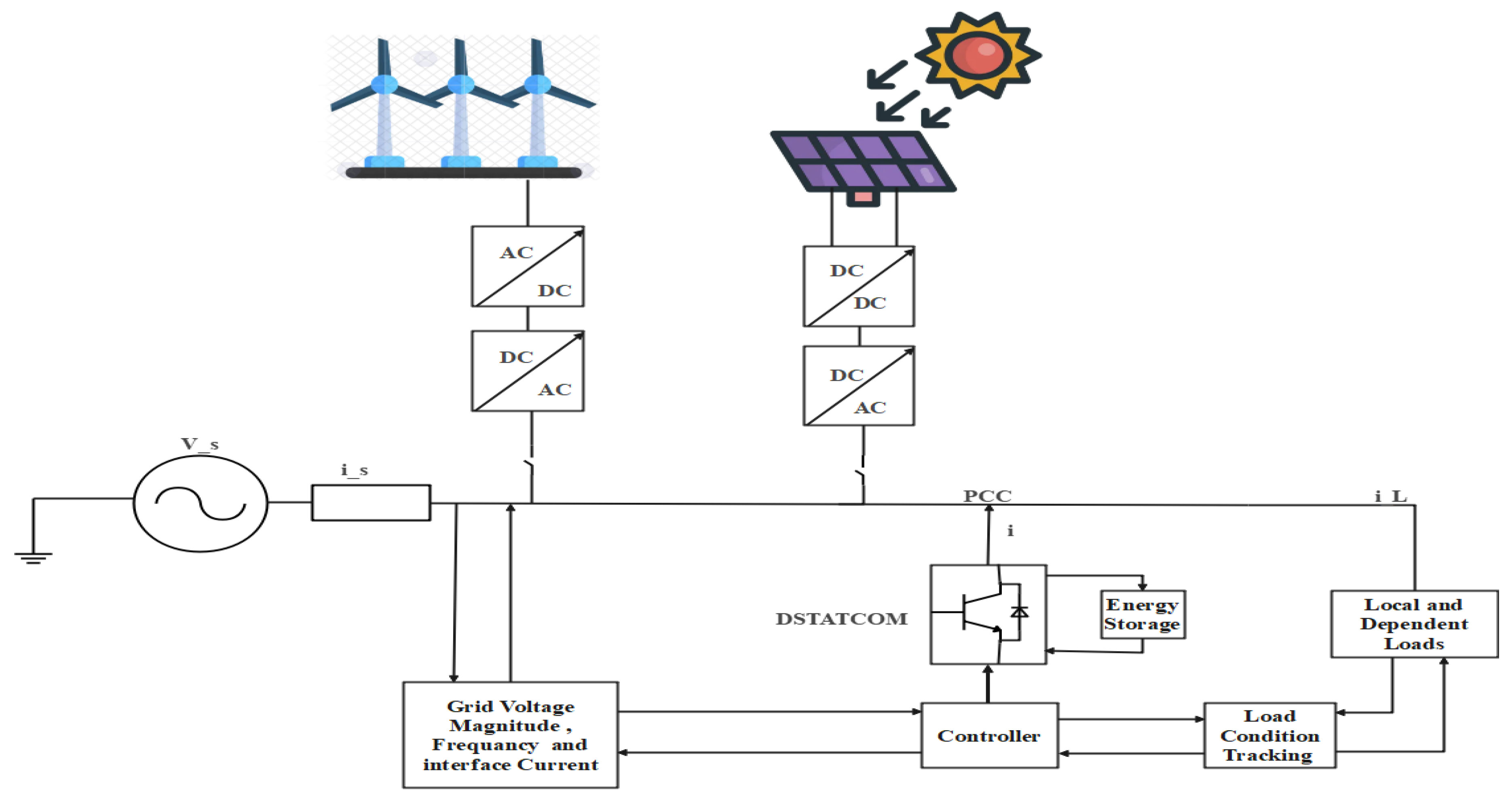
Figure 2.
Monthly average wind speed Measured at a reference hub height of 10 m.
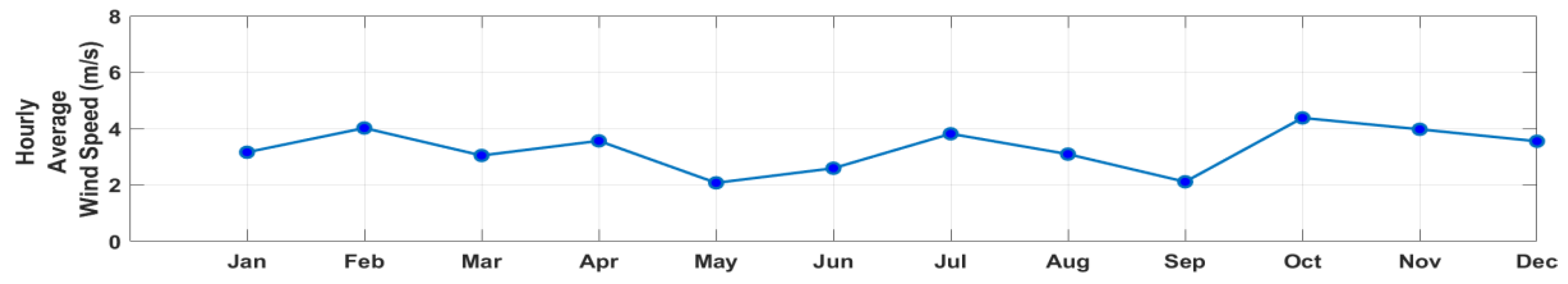
Figure 3.
Monthly average solar radiation.
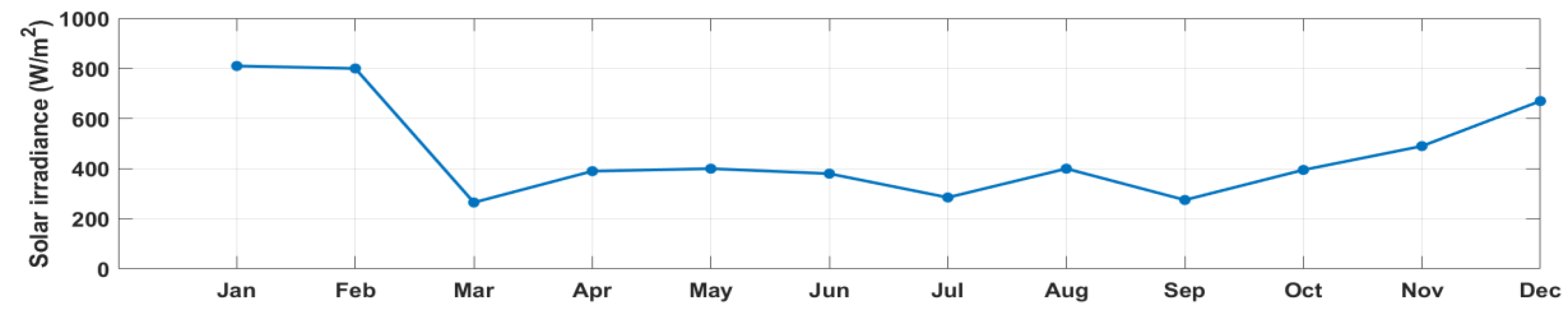
Figure 4.
The monthly minimum, average, and maximum ambient temperatures.
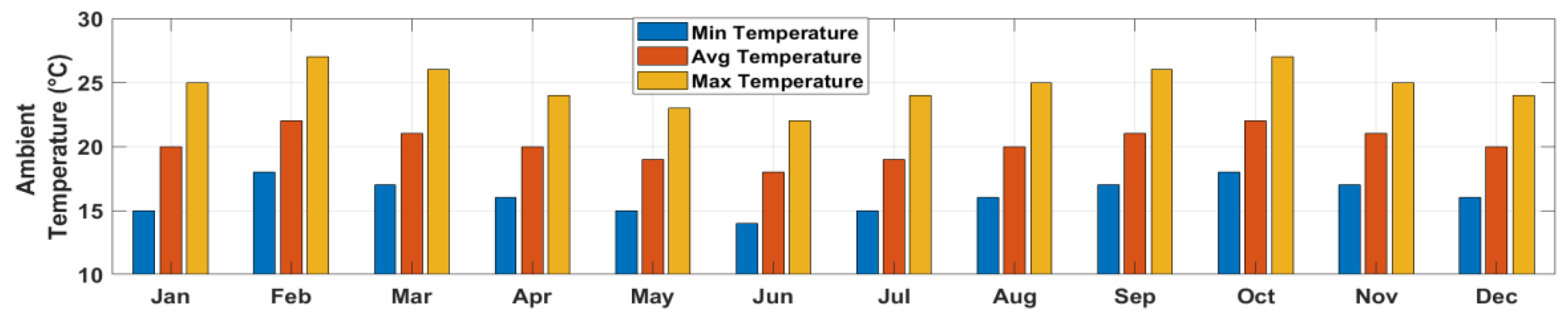
Figure 7.
Generation percentage contribution.
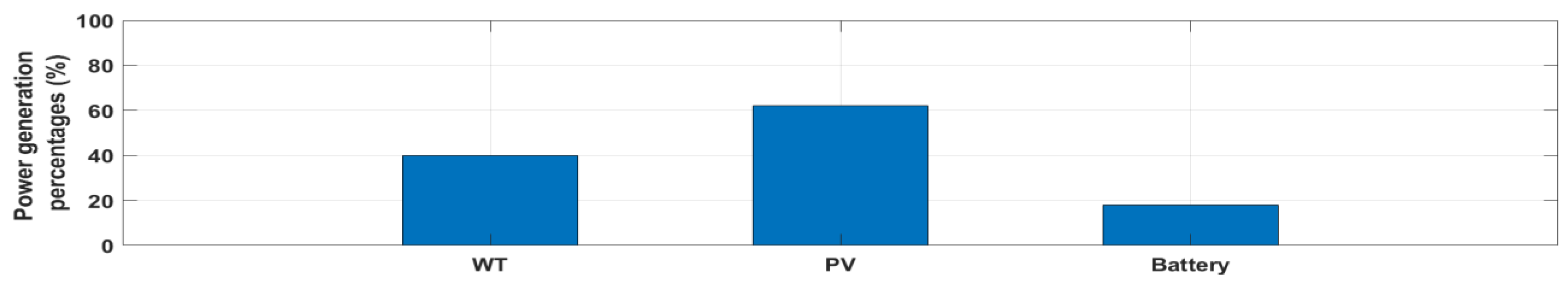
Figure 8.
percentages for cost allocation.
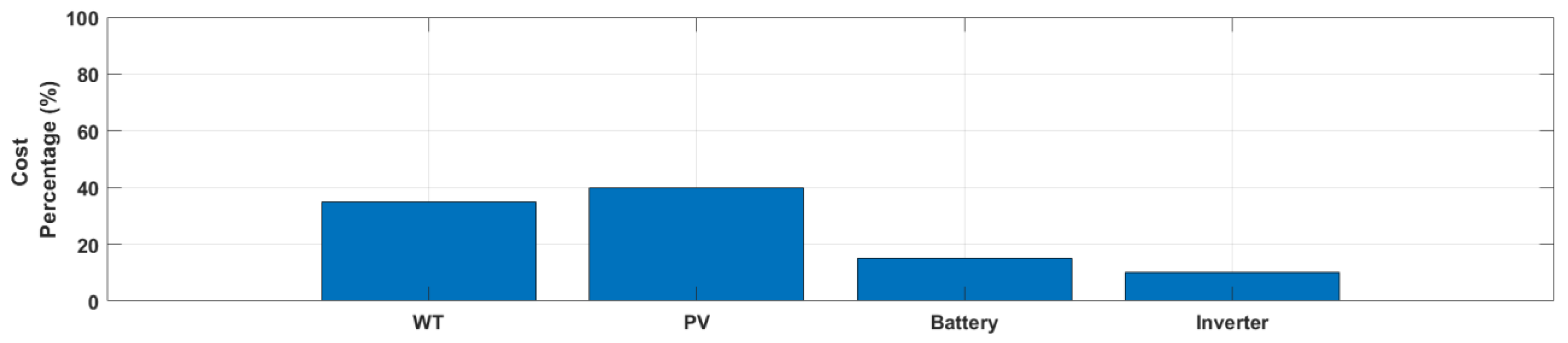
Figure 9.
Comparative analysis of voltage profiles before and after the integration of WT, PV, combined WT-PV, and WT-PV-DSTATCOM systems using HGA-PSO.
Figure 9.
Comparative analysis of voltage profiles before and after the integration of WT, PV, combined WT-PV, and WT-PV-DSTATCOM systems using HGA-PSO.
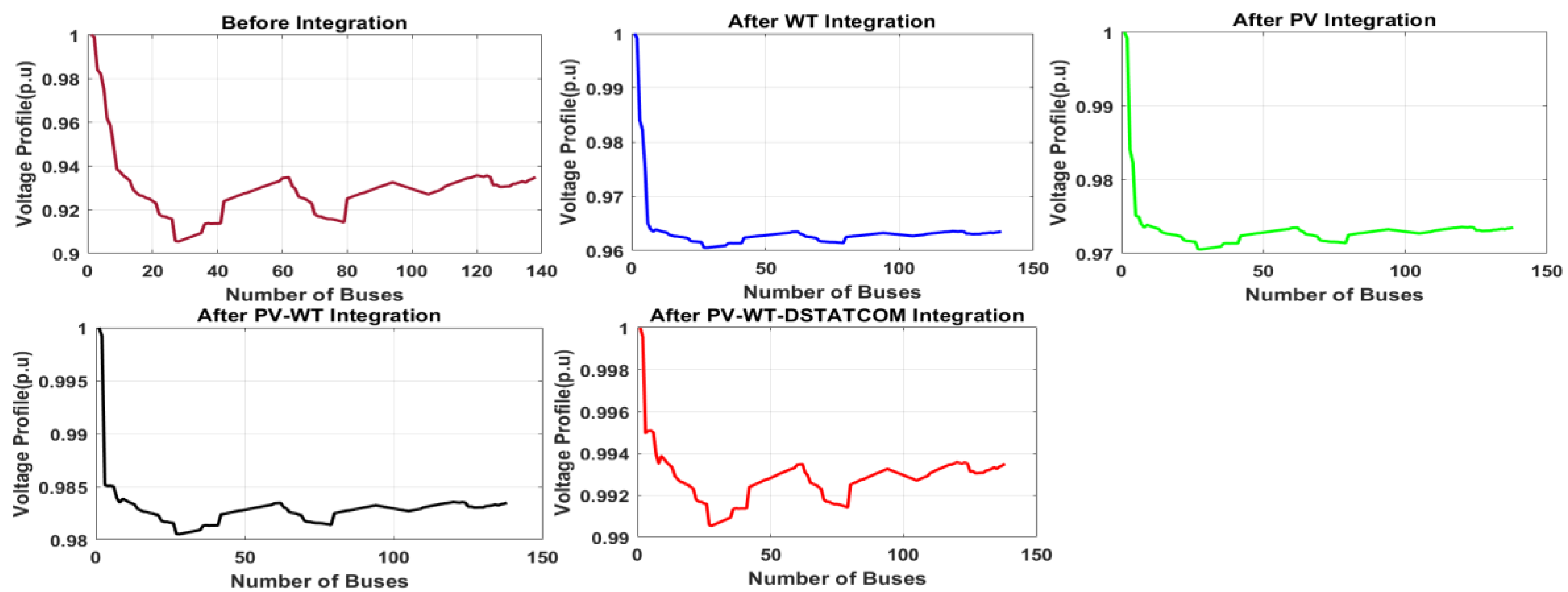
Figure 10.
Total Power Losses Under Different Scenario.
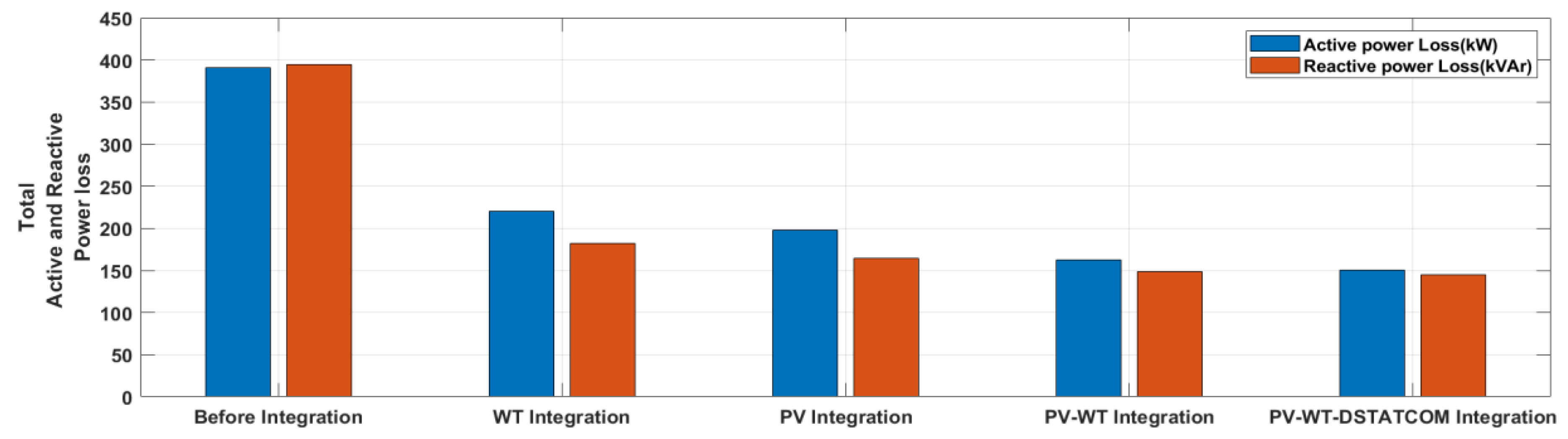
Figure 11.
Convergence Curves of Objective Function Value Under Different Scenarios Using HGA-PSO.
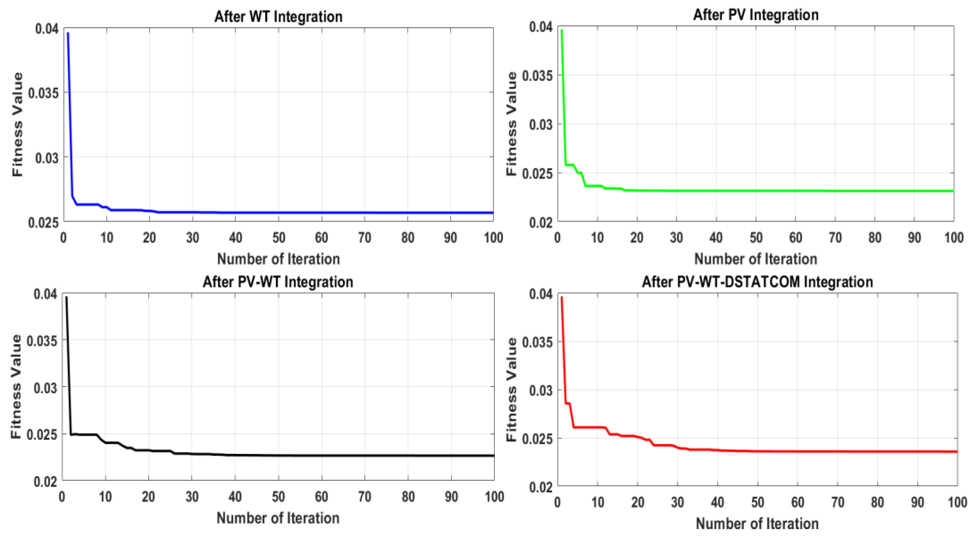
Table 3.
Result summary for all scenarios.
| Objectives | Before Integration |
After Integration | |||
| WT | PV | PV-WT | PV-WT-DSTACOM | ||
| Total active power loss (kW) | 390.9944 | 220.162 | 198.1035 | 162.6685 | 150.765 |
| Total active power loss red (%) | 43.69 | 49.33 | 58.39 | 61.44 | |
| Total reactive power loss (kVAr) | 394.895 | 182.60558 | 164.578 | 148.7415 | 145.2265 |
| Total reactive power loss red (%) | – | 53.76 | 58.32 | 62.33 | 63.22 |
| Minimum voltage (p.u.) | 0.9055 | 0.96055 | 0.97155 | 0.9821 | 0.99925 |
| Minimum V. deviation (%) | 9.45 | 3.945 | 2.845 | 1.79 | 0.075 |
| Fitness Values | – | 0.02569 | 0.02318 | 0.02366 | 0.02268 |
| LSF (p.u.) | 0.92023 | 0.216401 | 0.079056 | 0.059799 | 0.036588 |
| DG location | – | 105 | 127 | 41 | 28 |
| VSI (p.u.) | 0.05232 | 0.06939 | 0.478401 | 0.556126 | 0.581077 |
| DG size (kVAr) | – | 861 | 1206 | 2067 | 3630 |
| Percentage for Cost allocation | - | 35 | 40 | 75 | 85 |
Disclaimer/Publisher’s Note: The statements, opinions and data contained in all publications are solely those of the individual author(s) and contributor(s) and not of MDPI and/or the editor(s). MDPI and/or the editor(s) disclaim responsibility for any injury to people or property resulting from any ideas, methods, instructions or products referred to in the content. |
© 2025 by the authors. Licensee MDPI, Basel, Switzerland. This article is an open access article distributed under the terms and conditions of the Creative Commons Attribution (CC BY) license (https://creativecommons.org/licenses/by/4.0/).
Copyright: This open access article is published under a Creative Commons CC BY 4.0 license, which permit the free download, distribution, and reuse, provided that the author and preprint are cited in any reuse.


