Submitted:
12 August 2025
Posted:
18 August 2025
You are already at the latest version
Abstract
In the development of quantum mechanics in the 1920s both matrix mechanics (Born, Heisenberg and Jordon) and Schrödinger wave mechanics (Schrödinger) prevailed. These early cases corresponded to the quantum mechanics of particles. Matrix mechanics was found to lead directly to the Schrödinger equation and likewise, the Schrödinger equation could be used to derive the inverse problem for matrix mechanics. Later emphasis lay with the development of the dynamics of fields, where the classical field equations were quantized (see for example Weinberg). Today, quantum field theory is one of the most successful physical theories ever developed. One of the important properties of quantum mechanics is that it is linear (i.e. the Schrödinger equation is linear), leading to some confusion about how to treat the problem for nonlinear classical field equations. In the present paper we address the case of classical soliton equations which are exactly integrable in terms of the periodic/quasiperiodic inverse scattering transform. This means that all physical spectral solutions of the soliton equations can be computed exactly for these specific boundary conditions. Unfortunately, such solutions are highly nonlinear, leading to difficulties for solving the associated quantum mechanical problems. Here we develop a road to find the exact quantum mechanical solutions for soliton dynamics. To address this difficulty, we address a recently derived result for soliton equations, i.e. that all solutions can be written as quasiperiodic Fourier series. This means that soliton equations, in spite of their nonlinear solutions, are perfectly linearizable with quasiperiodic boundary conditions. We then invoke the result that soliton equations are Hamiltonian and we are able to show that the generalized coordinates and momenta are also quasiperiodic Fourier series, a generalized linear superposition law that is valid in the case of classical dynamics and is here extended to quantum mechanics. This simplification of Hamiltonian dynamics thus leads to matrix mechanics. This completes the main theme of our paper, i.e. that classical, nonlinear soliton field equations, linearizable with quasiperiodic Fourier series, can always be quantized in terms of matrix mechanics. Future work will be formulated in terms of the Schrödinger equation. This work guarantees that all classical, soliton field equations have an exact linearized form for their quantum mechanical properties.
Keywords:
classical solitons
; quantum solitons
; nonlinear field equations
; soliton interactions in quantum mechanics
1. Introduction
We investigate the quantum mechanics of classical soliton equations taken in the limit of microscopic scales. We consider the Korteweg-deVries (KdV) equation as a first example. To follow this investigation: (1) We discuss how KdV has solutions in terms of Riemann theta functions and the Its-Matveev formula of algebraic geometry, which we analytically modify to give multiply periodic Fourier series. Thus, soliton equations have general solutions given by a linear superposition law, which allows us to study both wave motion and soliton (particle like) motion using the same formulation. (2) We write the Hamiltonian form of KdV and show that the coordinates and momenta also have multiply periodic Fourier series solutions, an assumption first made by Heisenberg [1930] to derive matrix mechanics. (3) We find the Hamiltonian for KdV and show that it too is quasiperiodic. This leads to matrix mechanics. (4) We discuss the fact that the vacuum or ground state of both the classical and quantum mechanical problems, has temporal time behavior and can never be set to zero. (5) The study of the KdV equation given herein could be called the quantum Fermi-Pasta-Ulam (qFPU) problem whose original study [Fermi, Pasta and Ulam, 1955] let to the discovery of the soliton [Zabusky and Kruskal, 1965] and the inverse scattering transform (IST) [Gardner, Greene, Kruskal and Miura, 1967]. In the present paper we study the qFPU problem from the point of view of temporally quasiperiodic boundary conditions which employs our understanding of quantum finite gap theory [Faddeev and Takhtajan, 1987] [Belokolos, et al, 1994] [Gesztesy and Holden, 2003].
2. The KdV Equation and its Linear Superposition Law Solution
The KdV equation [Korteweg and deVries, 1895] describes shallow water waves, which in dimensional form is given by:
 (1)
(1)KdV is also at the foundations of the Fermi-Pasta-Ulam problem [1955] which resulted in the discovery of the inverse scattering transform [Gardner et al, 1967]. We consider the solution of KdV in terms of the Cauchy problem for which we assume the spatial initial conditions at time t = 0, u (x, 0), is given and the evolution is then found for all space and time, u (x, 0)⇒u (x, t). The coefficients of (1) have the usual expressions for shallow water waves
 (2)
(2)where co is the linear phase speed, h is the water depth and g is the acceleration of gravity (the mks system of units is assumed). The form of the KdV equation used by Gardner, Green, Kruskal and Miura [1967] (ut + 6uux + uxxx = 0) has coefficients:
 (3)
(3)And the form of the equation used by Gardner [1971] (ut + uux + uxxx = 0) has coefficients:
 (4)
(4)Finally, the coefficients used by Zabusky and Kruskal [1965] (ut + uux + δ2uxxx = 0) to discover the soliton were
 (5)
(5)We will use (2) throughout and thus it is easy to obtain and compare results with the other forms of KdV by (3)-(5).
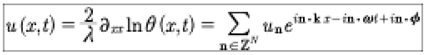
The quasiperiodic Fourier series solution of KdV has the form
 (6)
(6)where the second derivative of the logarithm of the Riemann theta function is called the Its-Matveev formula [Its and Matveev, 1975]. Here the solution of KdV is scaled by the parameter λ = α/6β, which keeps the solution in dimensional, physical units of meters and seconds.
For decades the form of the Its-Matveev formula in (6) has precluded applications of the finite gap method [Belokolos et al, 1994] [Gesztesy and Holden, 2003] for the study of stochastic solutions of the KdV equation [Osborne, 2010]. It is for this reason that Osborne [2018] sought a solution to this problem by writing the right hand side of (7) as a quasiperiodic Fourier series which is physically equivalent to the Its-Matveev formula on the left:
 (7)
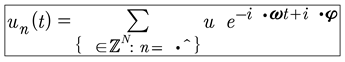
(7)The quasiperiodic Fourier series on the right of (7) is a generic linear superposition law for soliton equations [Osborne, 2018] [Osborne, 2019] [Osborne, 2020]. The Riemann theta function has the form:
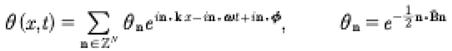 (8)
(8)Here B is the Riemann matrix. Equation (7) is a remarkable result, because it says that, in spite of the nonlinear behavior, the solutions of KdV can always be written by a linear superposition law. Thus we have the general soliton solution of the KdV equation whose solutions may be generally written with a quasiperiodic Fourier series solutions instead of the more traditional infinite line nonlinear soliton interactions. We refer to the linear superpositon law as a spectral solution of the KdV equation which is spectrally defined by the Riemann matrix: The diagonal elements are Stokes waves and the off-diagonal elements are pair wise interactions between the Stokes waves. The result (7) evidently generally holds true for all integrable soliton equations [Osborne, 2019]. Furthermore, the coefficients u are given explicitely in terms of the Riemann spectrum (the Riemann matrix written in terms of ):
 (9)
(9)Here the first equation corresponds to an inverse correlation constructed from the Its-Matveev formula [Osborne, 2018] and the second corresponds to three-wave interactions, well-known to describe KdV behavior. The following expressions for the coefficients of the theta function hold, which with (9) connects the Riemann spectrum B to the measurable field un(t):
 (10)
(10)for
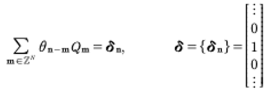 (11)
(11)Notice that in the first of (11) we are considering the product of two quasiperiodic Fourier series (resulting from an infinite dimensional matrix times an infinite length vector) such that their product is 1, here written on the right of (11) as an infinite vector whose only nonzero component is 1, found at the central postion.
This closes the connection between the general spectral solutions of KdV using finite gap theory [Its and Matveev, 1975] and the linear superposition law on the right of (7). Thus the right hand side of (7) solves the KdV equation for the Cauchy problem, just as does the Its-Matveev formula on the left hand side of (7). Of course the solutions (7) can be reduced to spatially periodic boundary conditions, as discussed below. Such solutions can also be viewed as “strings.” This gives an interpretation of (7) as an “infinite string,” because it is quasiperiodic, not periodic.
Are there any advantages for the quasiperiodic Fourier series in (7) over the Its-Mateev formula? For many physical applications we find that the quasiperiodic Fourier series solution of nonlinear wave equations makes all applications of integrable nonlinear pdes isomorphic to solving the Cauchy problem for linear pdes! Linear pdes use the periodic Fourier transform as as their solutions, for situations with well-defined dispersion. Thus, we have the possibility to study stochastic nonlinear waves using quasiperiodic Fourier series with random phases [Osborne, 2018a,b] [Osborne, 2019] [Osborne, et al, 2020]. Computation of the correlation function, power spectrum, coherence functions, etc. [Bendat and Piersol, 1986] are just as easily made for nonlinear equations as for linear equations using quasiperiodic Fourier series. This contrasts to the use of kinetic equations to study stochasticity in nonlinear waves [Hasselmann, 1972] which describe only weakly interacting sine waves. Equation (7) has instead all the modes of soliton theory, namely sine waves, Stokes waves, solitons, breathers, superbreathers, kinks, vortices, etc., all “coherent structure” solutions of integrable, nonlinear pdes. Thus (7) demonstrates that the natural modes of nonlinear pdes are these coherent structures, not just sine waves. This is the primary physical manifestation of nonlinearity in soliton wave equations. Many of the numerical methods for computing theta functions and quasiperodic Fourier series have been given in Osborne [2010] [Osborne, et al, 2018] where several data analysis methods are also presented.
The nonlinear dispersion relation for the KdV equation can be obtained by inserting the quasiperiodic Fourier series (7) into the KdV equation (1). One finds
 (12)
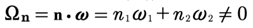
(12)where
 (13)
(13)The point set of frequencies n·ω (12) is often referred to as a discretuum [Bousso and Polchinski, 2000] because, while discrete, the point set is infinitely dense, essentially simultaneously approximating a continuum. The algebraic geometric form of the dispersion relation, equivalent to (12), (13), is discussed in [Osborne, 2010] [Osborne, 2018] where the algebraic geometric loop integrals are given, together with the relevant literature [Belokolos, et al, 1994] [Gesztesy and Holden, 2003].
3. The Spatially Periodic Solutions of the KdV Equation
It is often useful to assume spatially periodic boundary conditions for the KdV equation. For example Zabusky and Kruskal [1965] used these to develop the concept of the soliton in nonlinear wave theory. The study of the Fermi-Pasta-Ulam problem [1955] using the methods given herein might indeed be referred to as the “quantum FPU problem.” Using spatially periodic boundary conditions means that:
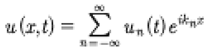 (14)
(14)Inserting this expression into the KdV equation gives a set of ordinary differential equations for the time evolution of the coefficients in the Fourier series (14):
 (15)
(15)where the linear dispersion relation is given by:
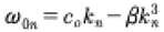 (16)
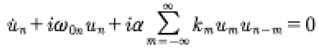
(16)Equation (15) can be written in a more convenient form:
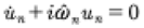 (17)
(17)where the associated nonlinear dispersion relation for the spatially periodic KdV equation thus has the form:
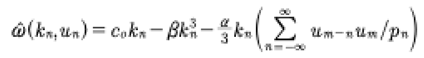 (18)
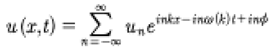
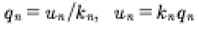
(18)It has been shown in [Osborne, 2010] [Osborne, 2018] that (7) can be reduced to (14) such that the Fourier coefficients themselves have a quasiperiodic Fourier series, which we write:
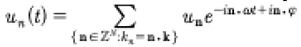 (19)
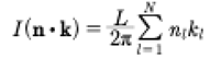
(19)It should be clear that (19) solves (15)! Equation (14) fixes the spatial evolution to be periodic, but the time evolution in this case is quasiperiodic (19) while governing soliton behavior. In summary: (19) used in (14) with the dispersion relation (18) solves the KdV equation. The reduction of (12), (13) to (18) occurs because we use spatially periodic boundary conditions as in (14). In this case we see that n·k⇒kn, i.e. because the wave numbers are commensurable (corresponding to spatial periodicity). Each dot product reduces to a wave number on the “basis set” of commensurable wave numbers k = [k1,k2…kN], kn = 2πn/L. The n·ω are nevertheless on the discretuum.
To better understand the notation given here, let us graph some of the spectral properties for the wavenumbers and frequencies. In the linear case, where α = 0, we have the spectra for the wavenumbers which are assumed to be commensurable and for the frequencies, by (14), are found to be incommensurable as shown in Fig. 1.
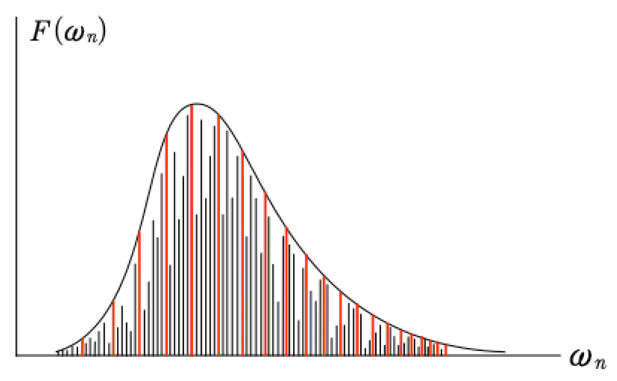
Because the wavenumbers are commensurable, their dot products with the integer summation vecters n are the same set of commensurable wave numbers: n·k⇒kn, although each is repeated an infinite number of times. As a consequence the frequencies are incommensurable and given by (18): The frequencies n·ω fall on a discretuum of points. Thus while they are discrete, they are nevertheless so densily packed as to blacken the spectral domain. We show graphically some of these frequencies, filling the region between the base frequencies (red), in Fig. 2.
Another convient way to represent the nonlinear spectrum of a quasiperiodic Fourier series is shown in Fig. 3. These are the “coherent modes” of the spectrum which consist of the Stokes waves. These contain the higher order harmonics, graphed perpendicular to the usual frequency axis and labeled the “bound frequencies”. The frequency axis itself refers to the “free” modes. Where is the discretuum shown in Fig. 2 to be found in Fig. 3? They lie on the frequency axis and densely fill the lines between the Stokes waves, thus constituting the “Stokes wave interactions.” In the soliton limit of the Stokes waves these interactions construct the “soliton phase shifts” as normally derived from infinite line soliton theory. The soliton behavior of (14) and (19) together provides a modern way to duplicate the numerical experiments of Zabusky and Kruskal [1962] for which the soliton was discovered. As a numerical model (14) and (19) have been referred to as “hyperfast” because of the enhanced speed of the algorithm with respect to traditional methods, see Chapter 32 of [Osborne, 2010].
Figure 1.
Commensurable wavenumbers (upper) and incommensurable frequencies (the so-called basis frequencies, lower panel, arising from (16)) for the linear problem, α = 0. Incommensurable basis frequencies manifest themselves as frequencies which are more closely spaced to the right of the spectrum, as shown in the bottom panel.
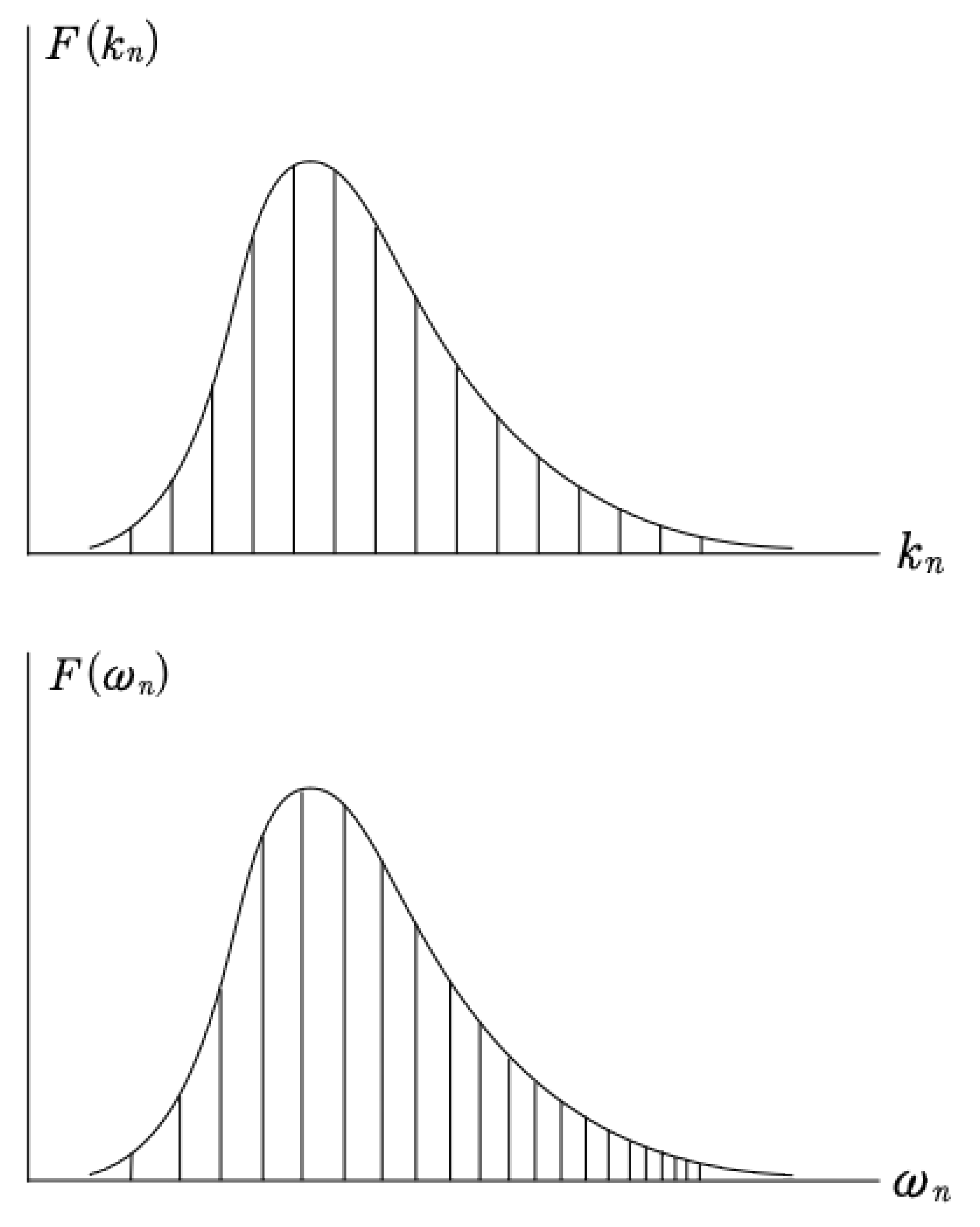
Figure 2.
Incommensurable basis frequencies (as shown in Fig. 01, lower panel) are here colored red to make them clear. The discretuum of frequencies (densely filling the regions between the red basis frequencies). These densely packeted frequencies constitute all the infinity harmonics in the spectrum. While the frequencies are themselves discrete, they are so dense as to approximate a continuum.
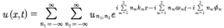
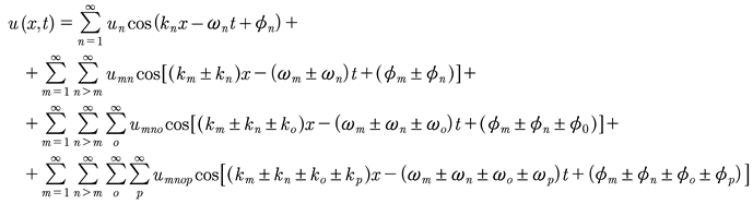
Here is an example of (7) for N degrees of freedom written as a nested summation (see also Chapter 7 of Osborne [2010]) for more details:
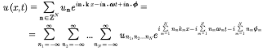 (20)
(20)This expression is just a representation of a genus N solution of the KdV equation, i.e. there are N modes consisting generally of a mixture of sine waves, Stokes waves and solitons, depending on how nonlinear each mode (each individual summation) is. The case for two degrees of freedom is given by:
 (21)
(21)This expression may be written as the sum of two solitons plus the nonlinear (phase shift) interactions. Of course a soliton is just a Stokes series for a single summation, provided that the elliptic modulus for each summation is sufficiently near 1.
Figure 3.
Another way to graph the quasiperiodic Fourier series spectrum in (7) is to view each nested sum in the quasiperiodic Fourier series spectrum as a Stokes wave, which then is associated with each incommensurable frequency. Each Stokes wave consists of several bound modes (mutually phase locked with each other) as shown in the graph. If a Stokes wave is small enough, then it effectively reduces to a simple sine wave because the higher harmonics are negligible. If a Stokes wave is large enough, the harmonics phase lock into a soliton. Two nearby Stokes waves that are phase locked with each other is a nonlinear wave packet (a nonlinear beat) otherwise known as a “fossil breather”, as shallow water manifestation of a deep water breather. Breathers are known to be a major source of rogue (giant) waves in the world ocean.

A single summation from the quasiperiodic Fourier series is given by:
 (22)
(22)This expression corresponds to a single Stokes wave: When the amplitude is small we have a sine wave, intermediate amplitudes give a traditional Stokes wave and if the amplitudes are large enough we have a soliton. Equations (9)-(11) determine how nonlinear each Stokes mode is and how strong their pair-wise interactions are. A single Riemann matrix diagonal element represents a soliton when the matrix element is sufficiently small and its elliptic modulus is thus sufficiently near 1 [Whitham, 1974] [Osborne, 2010]. The connection of the Rieman matrix elements and the soliton properties are given by (9)-(11) for the computations of the coefficients un1,n2…nN and for the amplitude dependent dispersion relation (18). Details are given in [Osborne, 2010] [Osborne, 2018].
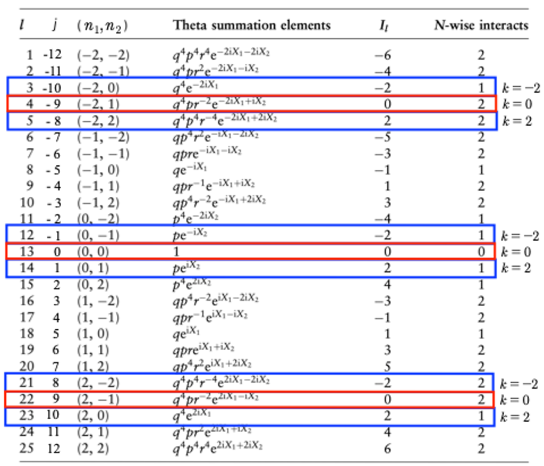
It is worthwhile looking at the details for a particular quasiperiodic Fourier series, which we write (see equation (21)):
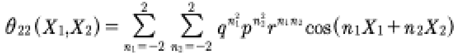 (23)
(23)For simplicity we have used limits of the two nested sums of -2, 2. This particular series is a Riemann theta function and we graph in Table 1 all the terms in the resultant “partial theta summation.” The Riemann matrix element corresponds to two degrees of freedom, with the Riemann matrix element being 2x2 (see the general forms (8), (21)). There are 25 terms in the partial summation and each is identified in the Table. The pairs of summation integers (n1, n2) are given in the third column. An ordering parameter j runs from -12,-11…-1,0,1…11,12 and is given in the second column. Each of the summation terms is given in the fourth column. By abuse of notation the term q = exp(−B11/2) (the first Stokes wave) corresponds to the first diagonal element of the Riemann matrix, while p = exp(−B22/2) (the second Stokes wave) corresponds to the second diagonal element and r = exp(−B12) corresponds to the off-diagonal element (which governs the interactions between the two Stokes waves).
In Fig. 4 we give a graph of the pairs of summation integers n=(n1, n2) as a function of the ordering parameter j (on the horizontal axis at the bottom). On the left vertical axis are the commensurable wavenumbers Il = n·k⇒kn, which run from -7,-6…-1,0,1…6,7. The zig-zag line, gives the actual terms summed as given in the Table 1. Each intersection of the zig-zag line corresponds to the crossing of a commensurable wavenumber Il = n·k⇒kn. Notice that for Il = n·k⇒kn = 0 we have the “ground state” (corresponding to the three red rectangles of Table 1) of the two-by-two quasiperiodic Fourier series: Note that there are three terms, the three red dots, that contribute three terms to the series. Also note that for Il = n·k⇒kn = 2 there are three blue dots, that contribute three terms to the series. For Il = n·k⇒kn = −2 there are another three blue dots, that contribute an additional three sine waves to the quasiperiodic Fourier series.
Of course any realistic summation will contains hundreds of thousands of terms, but such a case is not easily graphable. Now let us consider some examples of terms in this simple partial summation.
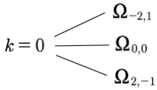
Simple Example #1
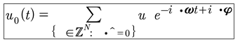
We see from Fig. 4 that for zero wavenumber k = 0 there are three integer vectors (-2,1), (0,0) and (2,-1) which give three terms that contribute to the Fourier series uo(t) (the zeroth, or ground state, term uo(t) in (14)) which have finite contributions. The three frequencies are computed from:
For which
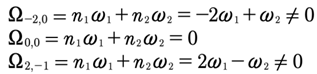
The three Fourier modes are shown in the three red boxes in the above Table 1 and the single red box in Fig. 4. Thus, in the present simple case the single wavenumber k = 0 corresponds to three frequencies. This result looks like line splitting in classical quantum mechanics, which is here done for the KdV nonlinear problem, but the results appear linear (they have been linearized) for the present example:
Figure 4.
Theta function partial sum for M = 2, N = 2. Here j = -12,-11,…11,12 and l=1,2…25.

Thus, the frequencies look like a line spectrum, the kind that scientists were studying in the 1920s (or for that matter, Newton studied in his investigation of optics in a prism). This case for ko = 0 corresponds to the zero or ground state, which is responsible for infra gravity waves in shallow water ocean waves.
Simple Example #2
We see from the figure above that for zero wavenumber k = 0 there are six integer vectors (-2,0), (0,-1), (2,-2), (-2,2), (0,1) and (20) which give six terms to the Fourier series (14) u2(t), u−2(t) which have finite contributions.
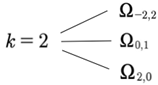
Then the six frequencies are computed and found to be, for k = 2:
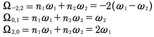
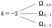
And for k = −2:
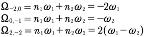
The six Fourier modes are shown in the six blue boxes in the above Table 1 and the two blue boxes in the Fig. 4. Thus, in the present simple case the single wavenumber k = 2 corresponds to three frequencies:
And for k = −2 we have three more:
From the last example we see that we get line splitting for an arbitrary selection of wave number. From these simple examples we see that each wavenumber Fourier component un(t) corresponds to each commensurable wavenumber kn= n·k (formally there are infinity of them, not just three as in the example of Table 1, Fig. 4), and hence there are an arbitrarily large numbers of frequency Fourier modes (essentially contributing to the discretuum), n·ω in any realistic physical situation. Typically, in a classical simulation of KdV we have several hundred thousand of these frequencies.
4. The Hamiltonian Form of the KdV Equation has Generalized
Coordinates and Momenta which are Quasiperiodic Fourier Series
If the spectral solutions of the KdV equation are quasiperiodic Fourier series as in the second equation of (7), then is it possible that the generalized coordinates and momenta of the Hamiltonian formulation of KdV are also quasiperiodic Fourier series? The reason that this question arises is that Born [1927], Born, Heisenberg and Jordon [1926], Born and Jorden [1925] and Heisenberg [1930] assumed “for simplicity” that the coordinates and momenta are given by quasiperiodic Fourier series (see discussion in the Appendix of Heisenberg [1930]). What followed from this assumption is the development of the matrix mechanics formulation of quantum theory (In modern work in quantum mechanics, one often uses an ordinary periodic Fourier series instead of a quasiperiodic Fourier series as suggested by Heisenberg. This assumption, although it may seem reasonable if one uses linearity as the basis of quantum mechanics, eliminates the important pathway to the integrability of soliton systems through Riemann theta functions and their linear superposition law derived from the Its-Matveev formula. Quasiperiodicity, remarkably, leads to the soliton dynamics of integrable wave equations.). Thus, should the Hamiltonian coordinates and momenta for the KdV equation be quasiperiodic Fourier series, then the matrix mechanics of the KdV equation would then follow in a natural way. We would therefore have quantum mechanics (a linear theory) valid for a nonlinear classical soliton equation! Thus our understanding of the quantization of nonlinear, classical wave equations would be improved, just by using our knowledge of finite gap itegration theory for soliton equations. Let us see if this is indeed the case.
The eventual goal of this work is to develop a kind of nonlinear quantum field theory (which we refer to as the quantum FPU problem), by first capturing the nonlinear dynamics of an integrable classical field equation using finite gap theory and then to quantize the associated soliton dynamics.
In the Appendix of his book Heisenberg [1930] suggests that one should address the Hamiltonian form of a classical physics problem and thereby seeks the associated quantum mechanics. He assumes in the beginning that the generalized coordinates and momenta have quasiperiodic Fourier series:
 (23)
(23) (24)
(24)where n = 1,2…N are the modes. Our modern perspective is that for soliton systems, quasiperiodicity implies integrability of the classical wave equation. It is amazing that Heisenberg selected soliton integrability in his “simple” solution of Hamilton’s equations and from this he developed matrix mechanics. While Born, Heisenberg and Jordon [xxxx] were dealing with systems of particles in their development of matrix mechanics, we now show that the generalized coordinates and momenta also appear as quasiperiodic Fourier series for soliton field equations, provided we address the Hamiltonian formulation of the KdV equations as first developed by Gardner [1971]. See also the book by Faddeev and Takhtajan [1987]. Applications of this method to quantum computing are discussed in Osborne [2023].
We now give a terse overview for the Hamiltonian form of the KdV equation. One begins with a classical variational principle which requires the definition of a functional:
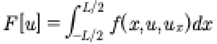 (25)
(25)We assume that the spatial variable x is on the interval (0,L) or (−L/2,L/2). In this expression f is viewed as a function of x, u and ux, such that u = u(x) and ux=du(x)/dx. We are familiar with the fact that we normally deal with the action integral where f is the Lagrangian and u(x) is mapped to the generalized coordinate q(t). This leads to the functional derivative
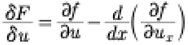 (26)
(26)Now, keeping in mind that the Hamiltonian, which is known to be related to the third conservation law of the KdV equation, has the form
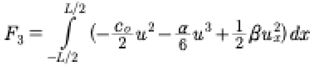 (27)
(27)We now find from (26), (27)
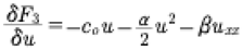 (28)
(28)Then the KdV equation (1) is determined from the Lagrangian by
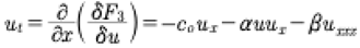 (29)
(29)In a straightforward derivation, the time derivative of the Fourier coefficients in (14), we find the form (see also (18) in [Gardner, 1971])
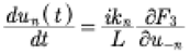 (30)
(30)It is then convenient to define the generalized coordinates, momenta and Hamiltonian as:
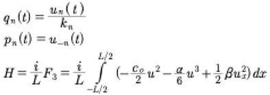 (31)
(31)This then leads to Hamilton’s equations:
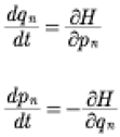 (32)
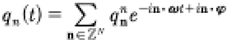
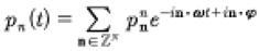
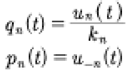
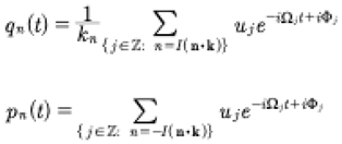
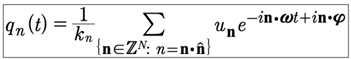
(32)From (19) and (31) we have the quasiperiodic Fourier series for the generalized coordinates and momenta for the KdV equation:
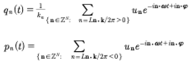 (33)
(33)Here n=1,2…N and Ln·k/2π=±n, for n a positive integer. We are summing over all n in this process, and when Ln·k/2π=+n we have contributions to qn(t). When Ln·k/2π=−n we have contribution to pn(t).
Now equations (33) may be written:
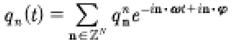 (34)
(34)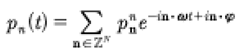
where the coefficients are related to the positive or negative integers
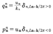 (35)
(35)and the Kronecker delta function is given by:
 (36)
(36)Thus we have found that for the KdV equation the generalized coordinates and momenta have quasiperiodic Fourier series, just as Heisenberg suggested.
5. Evaluation of the Gardner Formulation of the Hamiltonian for the KdV
Equation
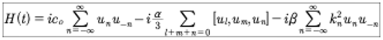
The Hamiltonian for the KdV equation, as already discussed above, is given in dimensional form by (see Gardner [1971], Feddeev and Takhtajan [1987]):
 (37)
(37)The constant coefficients in this expression are those of the KdV equation (1). To obtain the Hamiltonian for other forms of KdV, use the coefficients (2) - (5).
We note that many of the results of this paper are based upon the idea that one can add, subtract, multiply, divide, take derivatives and compute integrals of periodic and quasiperiodic Fourier series. The algebra and conditions for the validity of these operations are well known ([Zygmund, 1959] [Samoilenko, 1991], see also [Osborne, 2018, 2019]).
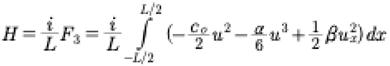
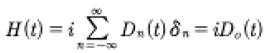
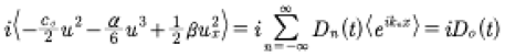
Now let us investigate how to compute this Hamiltonian integral (30). First let us suppose:
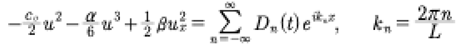 (38)
(38)where we determine Dn(t) below. To compute (38) with (14), (19) we need to momentarily let:
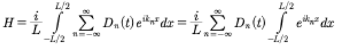 (39)
(39)Then the integral has the form:
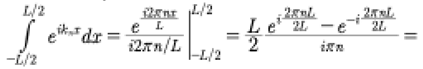 (40)
(40)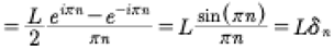 (41)
(41)Finally
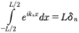 (42)
(42)This is the Kronecker delta function that came from the above integral:
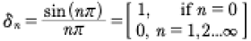 (43)
(43)for n, an integer. This is shown in the graph in Fig. 5.
Use this result in Eq. (39) to get:
 (44)
(44)This is equivalent to taking the mean
 (45)
(45)where the mean is given by
Figure 5.
This is a graph of equation (43)
as a function of continuous n. It is clear that for integer n the values are 1
for , and 0 for all
other (positive and negative) integers. Thus, we have the Kronecker.
Figure 5.
This is a graph of equation (43)
as a function of continuous n. It is clear that for integer n the values are 1
for , and 0 for all
other (positive and negative) integers. Thus, we have the Kronecker.
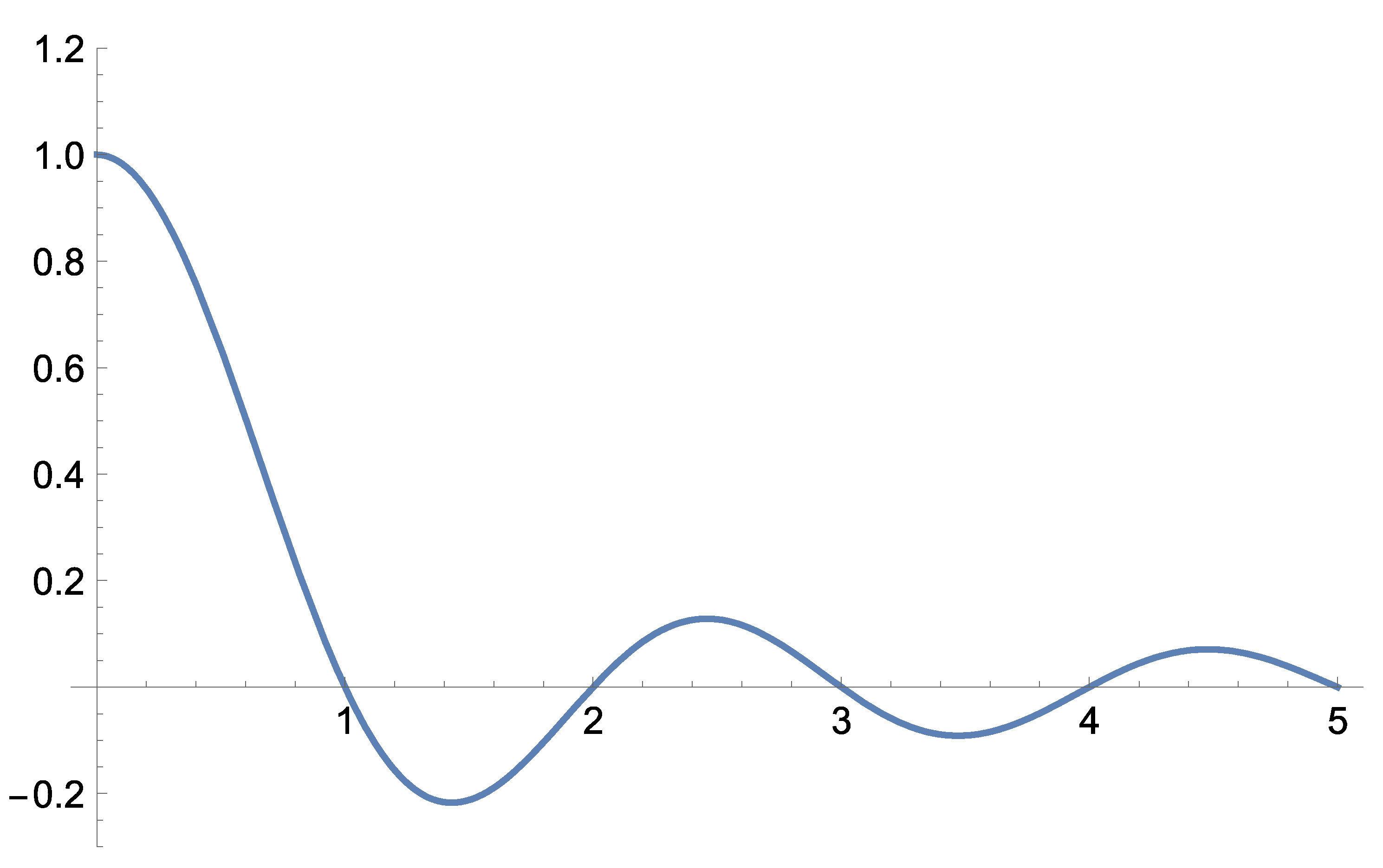
delta of Eq. (36).
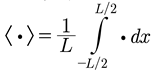 (46)
(46)Now let us compute the individual terms in the Hamiltonian (45).
First, the squared term is a simple convolution:
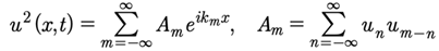 (47)
(47)
Proof:
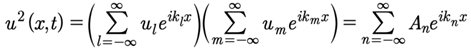 (48)
(48)where
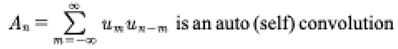 (49)
(49)Then, the cubic term is a double convolution:
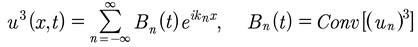 (50)
(50)
Proof:
 (51)
(51)where
 (52)
(52)From above (49) we have
 (53)
(53)Then, the squared derivative term is
 (54)
(54)Which gives
 (55)
(55)Then
 (56)
(56)We thus have the following results:
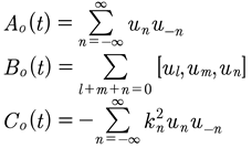 (57)
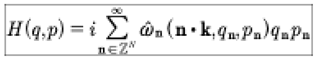
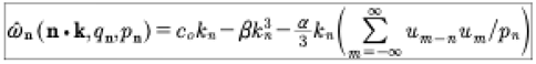
(57)This leads to the Hamiltonian in terms of the Fourier modes:
 (58)
(58)Here we have written the nonlinear term of the Hamiltonian as three wave interactions, which is physically expected for the KdV equation. In Hamiltonian mechanics it is often necessary to write: H(q,p,t). However, herein the form H(q,p) naturally occurs, as seen in the last equation. Note however that the un=un(t) and u−n=u−n(t) both depend implicitly on time. The lack of a direct temporal dependence in the Hamiltonian is important, particularly for writing the Hamiltonian-Jacobi equation and finding its solution, as will be discussed in a sequel paper. Using the coefficients un=un(t) and u−n=u−n(t) the Hamiltonian becomes:
 (59)
(59)Now use the following relation equating three wave interactions with a double convolution (see Appendix):
 (60)
(60)This gives the full Hamiltonian in terms of the Fourier spatial modes:
 (61)
(61)A simple change of variables gives:
 (62)
(62)Or
Now recall
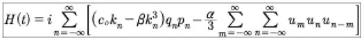
We finally have the Hamiltonian:
 (63)
(63) (64)
(64)Notice that the Hamiltonian has the same form as the linear problem, but now the dispersion relation is for the full nonlinear dispersion of the KdV equation. To arrive at the linear limit of the KdV equation we simply set α=0 to get the linear dispersion relation (16).
It is interesting to conjecture that the above expression for the Hamiltonian (63) suggests that all nonlinear, integrable wave equations can be written in this form. Thus, the Hamiltonian consists of a summation of terms with the nonlinear dispersion relation times the product of the generalized coordinates and momenta.
6. Matrix Mechanics for the KdV Equation
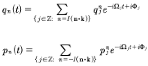
We take up here Heisenberg’s procedure [1930] which we apply to the quasiperiodic Fourier series given by (34)-(36). The approach was suggested by Osborne [2010] [2018] [2019] [2023] and requires that we write the quasiperiodic Fourier series for the generalized coordinates and momenta as a single summation, rather than as nested summations.
 (65)
(65)Here the index j is the ordering parameter used in Table 1 and Fig. 4. This enforces the limits −J≤j≤J on the above series. Furthermore, we compute J=[(2M+1)N+1]/2 where M is the limit of the nested summations and N is the number of nested sums. We use the definition
 (66)
(66)which fixes the meaning of the above summations. The frequencies and phases used above are defined by
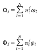 (67)
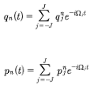
(67)The coordinates and momenta become
 (68)
(68)We then make the following choice
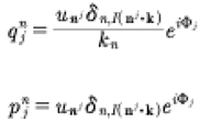 (69)
(69)where δ is the Kronecker delta. Finally, we have the simple expressions for the generalized coordinates and momenta.
 (70)
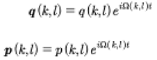
(70)At this point Heisenberg suggests that we write the coordinates in matrix form (see also Weinberg [2005]):
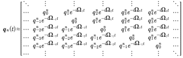 (71)
(71)Here we have used Heisenberg’s convention such that each row of the matrix contains sequential terms in the quasiperiodic Fourier series qn(t). Furthermore, each row is also shifted by one element so that the vacuum term always occurs on the matrix diagonal. It is further convenient to write the elements of the Heisenberg matrix as q(m,n). Then with this notation we have
 (72)
(72)The definition of the product of the two matrices has the form:
 (73)
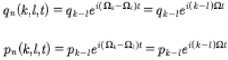
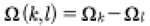
(73)At this point it is important to notice that the frequency Ω(k,l) associated with each coefficient q(k,l) then we can write the following expression:
 (74)
(74)This suggests that we must have an infinite array of incommensurable frequencies of the form:

Also note that
 (75)
(75)Because we are dealing with frequencies that are incommensurable so that the coordinates and momenta are quasiperiodic Fourier series. We also note that the q(k,l) are complex conjugates of the q(l,k).
We then find the following generalized coordinate matrix:
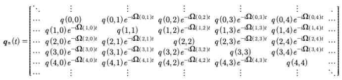 (76)
(76)The matrix of the momenta may also be written:
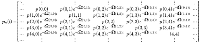 (77)
(77)It then follows that the commutator for q and p is given by:
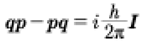 (78)
(78)This is of course one of the most fundamental relation of quantum mechanics, i.e. the noncommutativity of the coordinates and momenta in terms of Planck’s constant. It is well known that the latter expression is related to the uncertainty principle.
Heisenberg has made it clear that the matrices for the coordinates and momenta have the form:
 (79)
(79)These are the fundament matrices for the dynamics of the KdV equation, an important step for better understanding the quantum mechanics of this soliton equation in terms of finite gap theory.
7. Properties of Periodic Fourier Modes
The Hamiltonian is a constant for evolution described by the KdV equation. Time is not explicit in the Hamiltonian, but is implicit in the q’s and p’s. We see that the three-wave interactions are derived from the nonlinear term in the KdV equation. The time evolution of the Fourier modes un(t) is given by quasiperiodic Fourier series. We now look at some properties of these modes.
- Positive Fourier wavenumber components:
 (80)
(80)where the generalized coordinates and momenta are
Then the coordinates are
 (81)
(81)
The zeroth elements are uo(t),qo(t): This is the “dynamical ground state” which is a time varying background. It cannot be “turned off” by setting uo(t) to zero, except at t = 0. It seems to be a classical background state that turns into the “vacuum state” in the QM limit, where “particles” of various types pop up out of the vacuum.
 (82)
(82)We should recognize that uo(t) is formally the mean value of u(x,t). However, according to the latter equation the mean of this system is generally never zero, even in the classical case. In both the classical and quantum cases we see that the vacuum state is never zero and further has time dynamics in which nonlinear modes continually and spontaneously jump up out of the vacuum state.
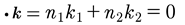
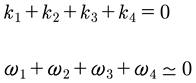
Let’s study the behavior of the vacuum state. We now show how this state can never remain zero, even if we arbitrarily set it to zero at time zero: u0(t=0)=0. This happens because we assume the wavenumbers are commensurable, but the frequencies cannot be zero because they are computed by the nonlinear dispersion relation: ωn(kn)=cokn−βk3n+n.l. The actual frequency is ·ω=n1ω1+n2ω2+…, which means ·k=n1k1+n2k2+…=0, k1=k, k2=2k. Let us consider the case for which n=[n1,n2]=[2,−1]. Then
 (83)
(83)but
 (84)
(84)We might say that generally speaking:
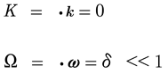 (85)
(85)These are the conditions that occur in nonlinear water wave resonances for zero wavenumbers and small frequencies. For the case of three-wave interactions (shallow water waves for the KdV equation) we have:
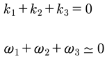 (86)
(86)For the case of four-wave interactions we have (in familiar notation for deep water, in terms of envelop equations such as the nonlinear Schrödinger equation, the Dysthe equation, the Trulsen-Dysthe equation… the Zakharov equation):
 (87)
(87)This reminds us that the quasiperiodic Fourier series can be written:
 (88)
(88)The terms with three-wave resonant interactions dominate in shallow water, while the four-wave resonant interactions dominate in deep water.
This above relation for uo(t) describes the vacuum state and the resonance conditions. It has a natural (slow) time evolution and thus can never be zero during the space time evolution of the KdV equation, even if we set it to zero at zero time. This is the familiar quantum mechanical result when the ground state has some finite value, never zero. It also says that even in the vacuum we get the constant occurrence (in the background) of the nonlinear modes (at long periods and short frequencies) that are derived from the “particle-like soliton” modes of the period matrix. The random appearing modes seem to be a kind of classical analog of the quantum modes jumping up randomly out of the vacuum state.
- Negative Fourier wavenumber components:
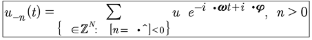 (89)
(89)where the momenta are:
Then the momenta are given by:
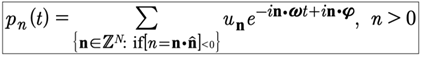 (90)
(90)8. Summary of the Results of This Paper on the Classical and Quantum KdV
Equations
- (1)
- In Osborne [2018], the odes for the un(t) (15) were solved analytically (19) by initially solving the KdV equation with quasiperiodic Fourier series, in both space and time. This was done with the Baker-Mumford theorem, inferring that the Its-Matveev formula could be expanded in terms of a quasiperiodic Fourier series whose coefficients are written in terms of the Riemann matrix by (9)-(11). We refer to this operation using the Baker-Mumford theorem as a kind of inverse convolution, i. e. the ratio of two theta functions and their derivatives is a general, single valued, multiply periodic, meromorphic function written in terms of Riemann theta functions.
- (2)
- The quasiperiodic Fourier series solution of KdV (7) is then written as periodic in space and quasiperiodic in time (14), (19) with nonlinear dispersion (18). It then follows naturally that the time varying Fourier coefficients (19) solve the set of odes for the Fourier coefficients un(t) (15).
- (3)
- We then discuss how Hamilton’s equations (30) (written as a function of the un(t)) are solved by the un(t) (19).
- (4)
- Formally the Hamiltonian can also be written in terms of the q’s and p’s with the solutions (33).
- (5)
- The fundamental generalized coordinates and moment for the quantum mechanical KdV equation have been computed in terms of the finite gap spectrum (the Riemann matrix) of the quasiperiodic inverse scattering transform.
- (6)
- The ground state of the KdV equation is found to never be zero, but instead is a time varying source of KdV modes determined from the Riemann spectrum.
- (7)
- We refer to the problem studied here as the quantum Fermi-Pasta-Ulam problem.
Appendix
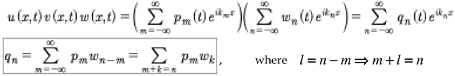
Properties of Products of Three Fourier Series
Consider three Fourier series:
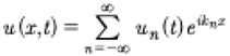 (A1)
(A1)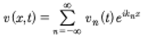 (A2)
(A2)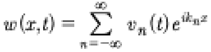 (A3)
(A3)where the wavenumbers are commensurate, kn=2πn/L, L the spatial period.
Now let us consider the triple product:
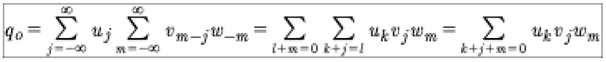
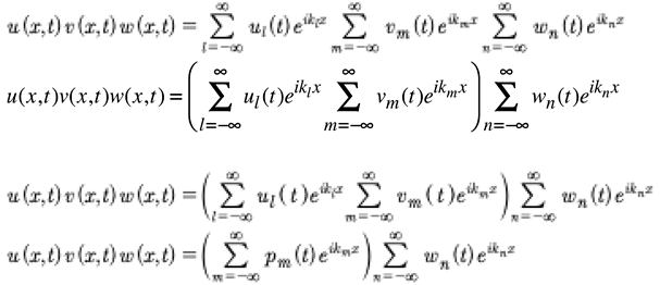 (A4)
(A4)where
 (A5)
(A5)The first notation is a simple convolution. The second notation is for two-wave interactions.
Now let us return to (III.4) to get the second convolution
 (A6)
(A6)Now combine (A.5) and (A.6)
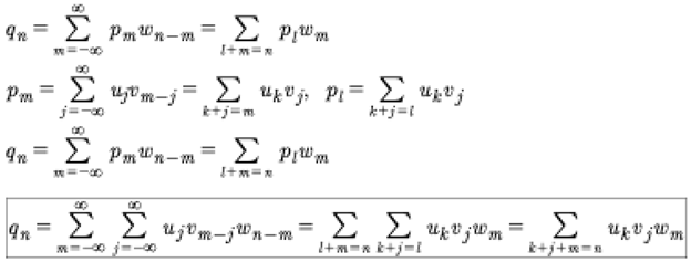 (A7)
(A7)We see that a double convolution leads to three-wave interactions.
The ground state of the triple product in (III.7) is an important result, set n=0, and is:
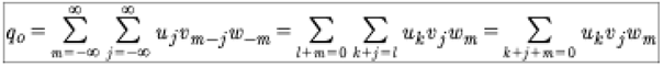 (A8)
(A8)In the case where we have the triple product of the same function, u3, for the ground state, we have from A.8:
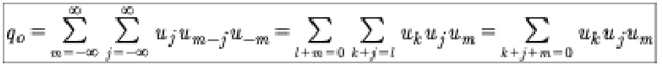 (A9)
(A9)Or
This result is used in the body of this paper to evaluate the nonlinear term in the Hamiltonian for the KdV equation.
Zygmund [1959] has discussed that the triple products of Fourier series are associative:
The triple product operations given above obey this associativity rule.
References
- Ablowitz, M. J. , and Segur, H., Solitons and the Inverse Scattering Transform, (SIAM, Philadelphia, 1981).
- Baker, H. F. , An Introduction to the Theory of Multiply Periodic Functions (Cambridge University Press, Cambridge, 1907).
- Belokolos, E. D. , Bobenko, A. I., Enol’skii, V. Z., Its, A. R., and Matveev, V. B., Algebro-Geometric Approach to Nonlinear Integrable Equations (Springer-Verlag, Berlin, 1994).
- Bendat, J. S. , and Piersol, A. G., Random Data: Analysis and Measurement Procedures (Wiley-Interscience, New York, 1986).
- Bousso, R. and J. Polchinski, Quantization of Four-form Fluxes and Dynamical Neutralization of the Cosmological Constant, J. High Energy Phys. 00006, April, 2000. [Google Scholar]
- Born, Max, The Mechanics of the Atom, (Bell and Sons, Ltd., London, 1927).
- Born, M. and Jorden, P., Zur Quantenmechanik. Zeitschrift fu, 1925; 34. [Google Scholar]
- Born, M. , Heisenberg, W., and Jorden, P., Zur Quantenmechanik II. Zeitschrift fu, 1926; 35. [Google Scholar]
- Born, Max, The Mechanics of the Atom, (Bell and Sons, Ltd., London, 1927).
- Costa, A., A. R. Osborne, D. T. Resio, S. Alessio, E. Chrivì, E. Saggese, K. Bellomo and C. E. Long, Soliton turbulence in shallow water ocean surface waves. Phys. Rev. Lett. 1085. [Google Scholar]
- Faddeev, L. D. and Takhtajan, L. A., Hamiltonian Methods in the Theory of Solitons (Springer, Berlin, 1987).
- Fermi, E. , Pasta, J. LA 1940, 1955. [Google Scholar]
- Gardner, C. S. , Greene, J. M., Kruskal, M. D., and Miura, R. M., Method for solving the Korteweg-deVries equation. Phys. Rev. Lett. 1967, 19, 1095. [Google Scholar] [CrossRef]
- Gardner, C. S. , Korteweg-deVries Equation and Generalizations. IV. The Korteweg-deVries Equation as a Hamiltonian System. J. Math. Phys. 1971, 12, 1548–1551. [Google Scholar] [CrossRef]
- Gesztesy, F. , and Holden, H., Soliton Equations and Their Algebro-Geometric Solutions, Volume I: (1+1)-Dimensional Continuous Models, (Cambridge University Press, Cambridge, 2003).
- Hasselmann, K. On the non-linear energy transfer in a gravity wave spectrum, Part 1. General theory. J Fluid Mech 1962, 12, 481500. [Google Scholar] [CrossRef]
- Heisenberg, W. , Über quantentheoretische Umdeutung kinematischer und mechanischer Beziehungen. Zeitschrift fu, 1925; 33. [Google Scholar]
- Heisenberg, W. , The Physical Principles of the Quantum Theory, (University of Chicago Press, Chicago, 1930).
- Its, A. R. , and Matveev, V. B., The periodic Korteweg-deVries equation. Funct. Anal. Appl.
- Korteweg, D. J. , and deVries, G., On the change of form of long waves advancing in a rectangular canal, and on a new type of long stationary waves. Philos. Mag. Ser. 1895, 5, 422–443. [Google Scholar] [CrossRef]
- Kuksin, S. B. 2000.
- Kuksin, S. B. , KAM-Persistence of Finite-Gap Solutions, in Dynamical Systems and Small Divisors, by L. H. Eliasson, S. B. Kuksin, S. Marmi and J.-C. Yoccoz, Springer, Berlin, 2002.
- Landau, L. D. , and Lifshitz, E. M., Quantum Mechanics: Nonrelativistic Theory, (Pergamon Press Ltd., London, 1958).
- Matveev, V. B. , 30 years of finite-gap integration theory. Phil. Trans. R Soc. A 2008, 366, 837–875. [Google Scholar] [CrossRef] [PubMed]
- Merzbacher, E. , Quantum Mechanics (John Wiley & Sons, New York, 1970).
- Mumford, D. , Tata Lectures on Theta II (Birkhäuser, Boston, 1984).
- Novikov, S. P. , Manakov, S. V., Pitaevskii, L. P., and Zakharov, V. E., Theory of solitons: The Inverse Scattering Method (Consultants Bureau, New York, 1984).
- Osborne, A. R. Nonlinear Ocean Waves and the Inverse Scattering Transform; Academic Press: Boston, MA, USA, 2010. [Google Scholar]
- Osborne, A. R. Nonlinear Fourier methods for ocean waves. Procedia IUTAM 2018, 26, 112–123. [Google Scholar] [CrossRef]
- Osborne, A. R. , Resio, D. T, Costa, A., de Leon, S. P, Chirivi’, E. Highly nonlinear wind waves in Currituck Sound: Dense breather turbulence in random ocean waves,. [CrossRef]
- Osborne, A. R. Breather Turbulence: Exact Spectral and Stochastic Solutions of the Nonlinear Schrödinger Equation. Fluids 2019, 4, 72. [Google Scholar] [CrossRef]
- Osborne, A. R. Theory of Nonlinear Fourier Analysis: The Construction of Quasiperiodic Fourier Series for Nonlinear Wave Motion, Offshore Mechanics and Arctic Engineering 2020, OMAE 2020-8536.
- Osborne, A. R. Nonlinear Fourier Analysis: Rogue Waves in Numerical Modeling and Data Analysis. J. Mar. Sci. Eng. 2020, 8, 1005. [Google Scholar] [CrossRef]
- Osborne, A. R. , Nonlinear Fourier Analysis Using Quasiperiodic Fourier Series, Offshore Mechanics and Arctic Engineering 2023, Melbourne, Australia, OMAE2023- 101978.
- Osborne, A. R. , Toward Quantum Algorithms for Simulating Nonlinear Ocean Surface Waves, Offshore Mechanics and Arctic Engineering 2023, Melbourne, Australia, OMAE2023-105072.
- Samoilenko, A. M. , Elements of the Mathematical Theory of Multi-Frequency Oscillations (Kluwer Academic Publishers, Dordrecht, 1991).
- Schrödinger, E. , Collected Papers on Wave Mechanics (Chelsea Publishing, New York, 1982).
- Weinberg, Stephen, The Quantum Theory of Fields, Volumes I, II and III (Cambridge University Press, Cambridge, 2005).
- Whitham, G. B. , Linear and Nonlinear waves (John Wiley, New York, 1974).
- Zabusky, N. J. , and Kruskal, M. D., Interaction of “solitons” in a collisionless plasma and the recurrence of initial states. Phys. Rev. Lett.
- Zygmund, A. , Trigonometric Series (Cambridge University Press, Cambridge, 1959).

Table 1.
Theta function partial sum for M = 2, N = 2.
 |
Disclaimer/Publisher’s Note: The statements, opinions and data contained in all publications are solely those of the individual author(s) and contributor(s) and not of MDPI and/or the editor(s). MDPI and/or the editor(s) disclaim responsibility for any injury to people or property resulting from any ideas, methods, instructions or products referred to in the content. |
© 2025 by the authors. Licensee MDPI, Basel, Switzerland. This article is an open access article distributed under the terms and conditions of the Creative Commons Attribution (CC BY) license (http://creativecommons.org/licenses/by/4.0/).
Copyright: This open access article is published under a Creative Commons CC BY 4.0 license, which permit the free download, distribution, and reuse, provided that the author and preprint are cited in any reuse.


