Submitted:
24 July 2023
Posted:
26 July 2023
You are already at the latest version
Abstract
Currently, two-component integrable nonlinear equations from the hierarchies of the vector nonlinear Schrodinger equation and the vector derivative nonlinear Schrödinger equation are being actively investigated. Usually, such two-component integrable nonlinear evolutionary equations are considered, the form of which does not depend on the replacement of one component with another. In this paper, we propose for consideration and usage a new hierarchy of two-component integrable nonlinear equations, which have an important difference from the already known equations. Among the hierarchy equations there are analogues of the two-component nonlinear Schrödinger equation (second equation from hierarchy) and the two-component modified Korteweg-de Vries equation (fourth equation from hierarchy). The third equation of the hierarchy is a combination of the nonlinear Schrödinger equation for one component and the modified Korteweg-de Vries equation for the second component. The equations for the individual components are very different from each other, even if they have the same order. Let us note that even hierarchy equations can be reduced to well-known variants of the scalar derivative nonlinear Schrödinger equations, and odd equations can’t be reduced. To construct the hierarchy equations, we use the monodromy matrix method, first proposed by B.A. Dubrovin. Knowledge of the monodromy matrix makes it possible to construct spectral curves of multiphase solutions, as well as to find stationary equations that these solutions satisfy. The last section presents the simplest solutions in the form of solitons and periodic one-phase waves, as well as spectral curves corresponding to these solutions.
Keywords:
spectral curve
; derivative NLS equation
; lax pair
; vector NLS equation
; monodromy matrix
Introduction
The transmission of information in the optical fiber is carried out by means of modulation of the reference laser signal. The fiber material is selected in such a way that the nonlinear effects resulting from the interaction of the wave with the medium compensate for the dispersion. The simplest model for the propagation of a polarized signal in an optical fiber is the focusing nonlinear Schrodinger equation
Here p is the slowly changing complex amplitude of the modulated signal superimposed on the laser reference wave, z is the coordinate along the direction of signal propagation, t is a linear combination of time and longitudinal coordinate (see, for example, [1] and references therein). It is not difficult to understand that equation (1) is an equation in dimensionless variables, i.e. it is obtained from the original equation by replacing variables and functions. This model is obtained from Maxwell’s equations by discarding terms that have little effect on the behavior of a nonlinear wave, i.e. it describes the real process with some accuracy [1]. The advantage of equation (1) is that it refers to integrable nonlinear equations (see, for example, [1,2,3,4,5,6]), which have solutions in the form of solitary waves (solitons). Solitons are nonlinear waves that propagate indefinitely without loss of shape and speed. Naturally, in real waveguides, solitons lose energy over time, but amplifiers and repeaters compensate for these losses. In the case of using lasers generating femtosecond pulses, the dispersion terms of the third, fourth and fifth order of the order must be taken into account in the models. These models correspond to the integrable Hirota equation [7,8,9,10]
and also integrable higher nonlinear Schrodinger equations [11,12,13,14]. There are also non-integrable models, which we will not discuss in this paper. To account for other types of interaction of waves with the waveguide medium, various variants of derivatives of nonlinear Schrödinger equations can be used [15,16,17,18,19,20,21,22,23,24,25,26,27,28,29,30,31,32,33], including the Kundu-Eckhaus equation [34,35,36]. Recently, models of waves with double polarization have been actively studied, since with the help of appropriate signals it is possible to transmit twice as much information [37,38,39,40,41,42].
Nonlinear signals are studied and filtered using a nonlinear Fourier transform [2,4,5,20,33,39,41,42,43,44,45,46,47]. In this case, spectral analysis is performed not of the nonlinear signal itself, but of the first operator from the Lax pair. Each simplest integrable nonlinear differential equation can be obtained as a condition for the compatibility of two linear differential equations, called a Lax pair [1,2,3,4,5,6]. In particular, the Lax pair for equation (1) has the form [1,2,3,4,5,6,48,49]
where , ,
, .
Note that each simplest integrable nonlinear equation is the first equation from an infinite sequence of equations called a hierarchy. Each equation from the hierarchy corresponds to its own second Lax pair operator. In particular, the nonlinear Schrodinger equation is the first equation from the Ablowitz-Kaup-Newell-Sigur hierarchy [48,49,50]. One of the useful features of hierarchies of integrable nonlinear equations is the fact that there are functions that satisfy all the equations of the hierarchy simultaneously. Hence, the functions will be solutions of the so-called mixed equations [11,12,13,14,48,49]. Therefore, consideration of the mixed equations is one of the ways to increase the number of integrable models of wave propagation in nonlinear media. Another way to construct new integrable models corresponding to the new properties of the studied nonlinear signals is to consider new Lax pairs. In particular, the propagation of bi-polarized waves in nonlinear optical waveguides is described by the Manakov system, which is a compatibility condition of linear matrix differential equations with third-order matrices [37,38,39,40,41,42,51,52,53,54,55,56]. Also, the compatibility conditions of Lax pairs with third-order matrices lead to two-component derivative nonlinear Schrödinger equations that describe more complex models of bi-polarized waves [57,58,59,60,61].
Naturally, all the models are regularly tested in practice when experimenters try to detect certain forms of signals obtained theoretically [62,63,64,65]. Therefore, one of the goals of theorists is to create new integrable models that could be used to describe nonlinear phenomena. In this paper, we propose for research a new integrable model describing the propagation of two interacting nonlinear waves
In the absence of one of the waves (), the model is reduced to the Gerdjikov-Ivanov equation [25,26,27,28,29,30,32,33]. The presented article consists of an introduction, five sections and concluding remarks. In the first section, we consider various possible variants of the Lax operator in the case of a quadratic spectral bundle. Based on the results of this section, we decided to investigate a model with a more general than usual Lax operator. The Section 2 of the paper is devoted to finding the structure of the monodromy matrix and the recurrent relations between its elements.
In Section 3, the stationary equations are derived and equations of spectral curves are considered. As in the case of the scalar derivative NLS equations [33], the stationary equations form two groups. But, if in the scalar case it was possible to use equations from only one group, then in the case of this model it is necessary to use both pairs of equations. Note also that in the case of usualy vector NLS equations [42,66], both components and satisfy similar stationary equations. In this paper, the components p and u satisfy stationary equations with different structures.
The Section 4 defines the sequence of the second equations from the Lax pair and the evolutionary integrable nonlinear equations from the corresponding hierarchy. Note that even hierarchy equations differ from odd ones. In particular, for we have
If we put in an odd equation, then it ceases to be an evolutionary integrable nonlinear equation. In Section 5 we present the simplest solutions of the second equation from the hierarchy we have constructed. In particular, we found a solution in the form of a solitary wave, the components of which are described by different formulas. This is due to the fact that each component satisfies its own nonlinear differential equation.
1. Structure of the Lax Operator for a Quadratic Spectral Bundle
Let the Lax pair be given by the equations
where
are constant matrices, is a spectral parameter.
The condition (5), along with integrable nonlinear equations, gives algebraic constraints on the elements of the matrices U and V. These restrictions have the following form
Usually solutions of the equation (7) is written using the relations
where R is some matrix of the same size.
Substituting (9) into (8) and simplifying, we get
or
Therefore, the following representation of the matrices and can be used
or
where is a new matrix of the same size. Note that in the right-hand sides of the equalities (9) and (10) it is possible to add linear combinations of matrices commuting with J and K.
Taking into account the remaining constraints from the condition (5) leads to the following matrix of operators (2) and (3)
where and are some functions. It is easy to see that the matrix J completely defines the structure of the operator (2). For example, if , then
In the case of the main variants of the derivative nonlinear Schrödinger equations, we have ()
By choosing other values of , other special cases of the generalized derivative nonlinear Schrödinger equation can be obtained [31,33,67,68,69]. Note that the solutions of these equations are connected by a gauge transformation preserving the amplitude (see for ex. [26,32,33,70,71,72]).
It is easy to notice that in these models, the matrices and depend only on two functions p and q, and the matrix is diagonal. Therefore, the addition of new functions u and v to the non-diagonal terms of the matrix allows us to explore a new nonlinear integrable model:
This model at is transformed into one of the special cases of the generalized derivative nonlinear Schrödinger equation [33]. The matrices J, and in the case of the new model are equal
2. The Monodromy Matrix
The monodromy matrix is a key object of spectral analysis of periodic solutions of the integrable nonlinear models. Spectral data in the case of periodic nonlinear signals is the spectral curve, its genus and its parameters. The equation of the spectral curve is the characteristic equation of the monodromy matrix M, which is a polynomial of the spectral parameter
and which satisfies the equation [73]
The monodromy matrix also exists in the limiting cases when the solution periods become infinite. In particular, solitary waves are the limiting cases of periodic waves when the period of a nonlinear wave becomes infinitely large.
From equation (13), where the matrix U is determined by the equalities (4), (12), the following structure of the matrix M follows
where , , ,
are some real constants. From Equation (6) it also follows the recurrence relations on the elements of the matrix :
In particular,
It follows from recurrent relations (15) that when the reality conditions
are met, the elements of the monodromy matrix satisfy the following relations
3. Conservation Laws
Conservation laws are described by the following stationary nonlinear differential equations
and
These equations also follow from equation (13).
Any m-phase solution for and for all values of t and z satisfies these stationary equations. The parameters of the corresponding multiphase solution depend on the constants and coefficients of the spectral curve (see below). It follows from the realness conditions (17) that stationary equations admit reduction (16).
In particular, for , the stationary equations have the form
It is easy to see that for , the components u and v are connected to the components p and q using the following relations
As will be shown below, in this case all components are expressed in terms of elliptic functions or their degenerations. Note that for , the system of stationary equations (18) splits into two separate identical systems, the solutions of which are plane waves. Accordingly, when , additional components can be removed from the model by putting .
Recall that the characteristic equation of the monodromy matrix M is the equation of the corresponding spectral curve
Here I is identity matrix. It follows from the equations (14) and (19) that the equation of the spectral curve has the form
where are constants (integrals). Therefore, the spectral curve is a hyperelliptic curve of genus . Naturally, this statement is true only for equations corresponding to non-degenerate connected curves.
For n=0 (g=1), the equation of the spectral curve has the form
where the integrals and are equal
I.e., for , the nondegenerate spectral curve is elliptic.
For (), the stationary equations have a more complex form
It follows from the first two equations of system (21) that in the case , the dependence of the components u and v on p and q can be found from the solution of the following linear matrix differential equation
It is easy to see that for , this equation admits solutions of the form . In this case, the stationary equations for the components p and q will take a simpler form
At the same time, it is not difficult to see that for there are solutions of stationary equations (21) that satisfy the condition .
The equation of the spectral curve for has the form
where the integrals , and are equal
For (), the stationary equations become even more complicated
It is easy to see that for , the dependence between the components and is described by nonlinear equations. At the same time, these equations also allow solutions of the form for . The equations for the components p and q in this case have the form
We will omit the values of the coefficients in the equation of the spectral curve for , since they are very cumbersome and are not interesting at the moment.
4. Integrable Nonlinear Evolutionary Equations
Let the second equation of the Lax pair have the form
where , or .
Then from the compatibility condition of the equations (2) and (24) the following evolutionary equations
follow.
It is not difficult to see that the evolutionary equations (25), as well as the stationary equations, admit reduction (16). Accordingly, after replacing (16), an integrable nonlinear two-component equation with a different dependence of the components on the variables will be obtained from the system of equations (25). Note that the well-known two-component integrable nonlinear equations [37,38,40,41,42,51,52,53,54,55,56,57,58,59,60,61] describe models with identical dependencies of components on variables .
We present the first evolutionary integrable equations from the corresponding hierarchy. For , the structure of the first two equations of the system differs from the structure of the last two:
Note that the last two equations of the system (26) when performing reduction (16) are analogous to the derivative nonlinear Schrödinger equation. At the same time, the first two equations describe a fairly simple relationship between the components.
For , the evolutionary equations have the form
It is easy to see that equations (27) are analogs of the two-component coupled derivative nonlinear Schrödinger equation. Assuming and , we obtain from equation (27) a new two-component derivative nonlinear Schrödinger equation
Unlike the usual vector derivative nonlinear Schrödinger equation [57,58,59,60,61], in this case the evolution of the components p and u is described by different equations.
For , the evolutionary equations again divided into two groups. The first two equations are analogs of the nonlinear Schrodinger equation, and the second are analogs of the modified Korteweg–de Vries equation
Assuming and , we obtain from equation (29) a two-component mixed equation
First equation is an analogue of the derivative NLS equation, and second equation is an analogue of the modifief Korteweg-de Vries equation.
Note that further the structure of the evolutionary equations (25) will depend on the parity of the number of the equation. For odd k, the order of derivatives with respect to t will be different, for even k, the same. In particular, for , the system of evolutionary equations will be an analogue of the vector modified Korteweg-de Vries equation. Note also that even equations admit reduction , whereas odd ones do not. In this case, equations (27) under this reduction and under condition (16) pass into the Gerdjikov-Ivanov equation [25,26,27,28,29,30,32,33]. I.e., the model considered in this paper generalizes the already known integrable models of nonlinear wave propagation.
5. One-Phase Solutions
To show differences in components behaviors, we consider examples with and . To find solutions to system (26), we express u and v from its first two equations and substitute them into the rest. After simplification we have
Let us note that equation (30) differs from equations (22) and (23).
Following [74], we will make a replacement in these equations
where
After simplification we have
Here is an integration constant.
Additional relations follow from the equation of the spectral curve. Converting expressions for constants and using substitutions (31) and (32), we obtain
It is not difficult to check the compatibility of the equations (33) and (34). It follows from these equations that the function is an elliptic function or one of its degenerations.
In particular, if the spectral curve is given by equation
then the constants and have the following values
For these values of constants, the function satisfies the equation
Solving this equation, we have
In this case
Substituting this value of the functions and into formulas (31) and (27), we get the solution to the equations (27)
where
It is easy to see that the components of solution (35) satisfy the reduction and . The amplitudes of the components p and u for , are shown in Figure 1.
It is not difficult to see that the shape of the component u is quite different from the shape of the component p. The component p is a classical soliton. At the same time, the component u is defined using a completely new expression.
Assuming , , it is possible to construct three different solutions in elliptic Jacobi functions [75,76].
If , then the function r(t) is expressed in terms of the :
The spectral curve of this solution is determined by the equation
where
In this case
where
Since the solution (37) to the equations (27) satisfies the conditions , , it is not suitable for describing the propagation of nonlinear optical signals.
When the function has the form
The spectral curve is again determined by equation (36). Only the branching points in this case are not real, but complex conjugate
The following periodic solution to the equations (27) corresponds to this curve:
where
Since reductions , are performed, solution (38) can be used to describe the propagation of a periodic nonlinear two-component wave. The amplitudes of the components p and u for , are shown in Figure 2. It is easy to see that the component p is an ordinary “dnoidal” wave, while component u has a non-standard shape.
The third elliptic solution to the equations (27) for is expressed in terms of the [75,76]:
and
where
The spectral curve of the solution (39) is given by equation (36), where
The examples we have considered have shown that, as in the case of the standard nonlinear Schrödinger equation, the location of the branching points of the spectral curve corresponds to the sign of reduction. If , then the branching points are on the real axis. If , then the branching points form complex conjugate pairs.
Concluding Remarks
From (15) and (25) the following equality
follows. Therefore, there exists the function such that
Note that the same statement is also true for other hierarchies (see, for example, [42,66,77,78]). As it was shown in [66], using equation (40), it is possible to construct a new vector analogue of the Kundu-Eckhaus equation.
Funding
The research was supported by the Russian Science Foundation (grant agreement No 22-11-00196)
Conflicts of Interest
The author declares no conflict of interest.
References
- Akhmediev, N.N.; Ankiewicz, A. Solitons, Nonlinear Pulses and Beams; CHAPMAN & HALL, 1997; p. 336. [Google Scholar]
- Ablowitz, M.J.; Segur, H. Solitons and the inverse scattering transform; SIAM: Philadelpphia, 1981; p. 425. [Google Scholar]
- Dodd, R.; Eilbeck, J.C.; Gibbon, J.D.; Morris, H.C. Solitons and nonlinear wave equations; Academic Press, Inc., 1982; p. 648. [Google Scholar]
- Calogero, F.; Degasperis, A. Spectral transform and solitons: tools to solve and investigate nonlinear evolution equations; North-Holland Publ. Comp.: Amsterdam, New York, Oxford, 1982; p. 516. [Google Scholar]
- Zakharov, V.E.; Manakov, S.V.; Novikov, S.P.; Pitaevskii, L.P. Theory of solitons. The inverse scattering method; Plenum, N.Y., 1984; p. 276. [Google Scholar]
- Faddeev, L.D.; Takhtajan, L.A. Hamiltonian Methods in the Theory of Solitons; Springer Ser. Classics in Mathematics, Springer, 2007; p. 585. [Google Scholar]
- Hirota, R. Exact envelope-soliton solutions of a nonlinear wave equation. J. Math. Phys. 1973, 14, 805–809. [Google Scholar] [CrossRef]
- Dai, C.Q.; Zhang, J.F. New solitons for the Hirota equation and generalized higher-order nonlinear Schrödinger equation with variable coefficients. J. Phys. A 2006, 39, 723–737. [Google Scholar] [CrossRef]
- Ankiewicz, A.; Soto-Crespo, J.M.; Akhmediev, N. Rogue waves and rational solutions of the Hirota equation. Phys. Rev. E 2010, 81, 046602. [Google Scholar] [CrossRef]
- Li, L.; Wu, Z.; Wang, L.; He, J. High-order rogue waves for the Hirota equation. Ann. Phys. 2013, 334, 198–211. [Google Scholar] [CrossRef]
- Wang, L.H.; Porsezian, K.; He, J.S. Breather and rogue wave solutions of a generalized nonlinear Schrödinger equation. Phys. Rev. E 2013, 87, 053202. [Google Scholar] [CrossRef]
- Ankiewicz, A.; Akhmediev, N. High-order integrable evolution equation and its soliton solutions. Phys. Lett. A 2014, 378, 358–361. [Google Scholar] [CrossRef]
- Chowdury, A.; Krolikowski, W.; Akhmediev, N. Breather solutions of a fourth-order nonlinear Schrödinger equation in the degenerate, soliton, and rogue wave limits. Phys. Rev. E 2017, 96, 042209. [Google Scholar] [CrossRef]
- Chowdury, A.; Kedziora, D.J.; Ankiewicz, A.; Akhmediev, N. Breather solutions of the integrable quintic nonlinear Schrödinger equation and their interactions. Phys. Rev. E 2015, 91, 022919. [Google Scholar] [CrossRef] [PubMed]
- Kaup, D.J.; Newell, A.C. An exact solution for a Derivative Nonlinear Schrödinger equation. J. Math. Phys. 1978, 19, 798–801. [Google Scholar] [CrossRef]
- Kamchatnov, A.M. New approach to periodic solutions of integrable equations and nonlinear theory of modulational instability. Physics Reports 1997, 286, 199–270. [Google Scholar] [CrossRef]
- Geng, X.G.; Li, Z.; Xue, B.; Guan, L. Explicit quasi-periodic solutions of the Kaup-Newell hierarchy. J. Math. Anal. Appl. 2015, 425, 1097–1112. [Google Scholar] [CrossRef]
- Arshed, S.; Biswas, A.; Abdelaty, M.; Zhou, Q.; Moshokoa, S.P.; Belic, M. Sub pico-second chirp-free optical solitons with Kaup-Newell equation using a couple of strategic algorithms. Optik 2018, 172, 766–771. [Google Scholar] [CrossRef]
- Jawad, A.J.M.; Al Azzawi, F.J.I.; Biswas, A.; Khan, S.; Zhou, Q.; Moshokoa, S.P.; Belic, M.R. Bright and singular optical solitons for Kaup-Newell equation with two fundamental integration norms. Optik 2019, 182, 594–597. [Google Scholar] [CrossRef]
- Smirnov, A.O.; Filimonova, E.G.; Matveev, V.B. The spectral curve method for the Kaup-Newell hierarchy. IOP Conf. Ser.: Mat. Sci. Eng. 2020, 919, 052051. [Google Scholar] [CrossRef]
- Ahmed, H.M.; Rabie, W.B.; Ragusa, M.A. Optical solitons and other solutions to Kaup-Newell equation with Jacobi elliptic function expansion method. Analysis and Math. Phys. 2021, 11, 23. [Google Scholar] [CrossRef]
- Chen, H.H.; Lee, Y.C.; Liu, C.S. Integrability of nonlinear Hamiltonian systems by inverse scattering method. Special issue on solitons in physics. Physica Scripta 1979, 20, 490–492. [Google Scholar] [CrossRef]
- Guo, B.; Ling, L.; Liu, Q.P. High-Order Solutions and Generalized Darboux transformations of derivative nonlinear Schrödinger equations. Studies in Appl. Math. 2013, 130, 317–344. [Google Scholar] [CrossRef]
- Yang, B.; Zhang, W.-G., Z. H.Q.; Pei, S.B. Generalized Darboux transformation and rational soliton solutions for Chen–Lee–Liu equation. Appl. Math. Comput. 2014, 242, 863–876. [Google Scholar]
- Zhang, Y.S.; Guo, L.J.; He, J.S.; Zhou, Z.X. Darboux transformation of the second-type derivative nonlinear Schrödinger equation. Lett. Math. Phys. 2015, 105, 853–891. [Google Scholar] [CrossRef]
- Peng, W.; Pu, J.; Chen, Y. PINN deep learning for the Chen-Lee-Liu equation: Rogue wave on the periodic background. Commun. Nonlinear Sci. Numer. Simul. 2022, 105, 106067. [Google Scholar] [CrossRef]
- Gerdjikov, V.S.; Ivanov, M.I. The quadratic bundle of general form and the nonlinear evolution equations. I. Expansions over the “squared” solutions are generalized Fourier transforms. Bulgarian J. Phys. 1983, 10, 13–26. [Google Scholar]
- Gerdjikov, V.S.; Ivanov, M.I. A quadratic pencil of general type and nonlinear evolution equations. II. Hierarchies of Hamiltonian structures. Bulgarian J. Phys. 1983, 10, 130–143. [Google Scholar]
- He, J.; Xu, S. The rogue wave and breather solution of the Gerdjikov-Ivanov equation. J. Math. Phys. 2012, 53, 03507. [Google Scholar]
- Guo, L.; Zhang, Y.; Xu, S.; Wu, Z.; He, J. The higher order Rogue Wave solutions of the Gerdjikov-Ivanov equation. Phys. Scripta 2014, 89, 035501. [Google Scholar] [CrossRef]
- Kundu, A. Landau-Lifshitz and higher-order nonlinear systems gauge generated from nonlinear Schrödinger-type equations. J. Math. Phys. 1984, 25, 3433–3438. [Google Scholar] [CrossRef]
- Xu, S.; He, J.; Wang, L. The Darboux transformation of the derivative nonlinear Schrödinger equation. J. Phys. A 2011, 44, 305203. [Google Scholar] [CrossRef]
- Smirnov, A.O. Spectral curves for the derivative nonlinear Schrödinger equations. Symmetry 2021, 13, 1203. [Google Scholar] [CrossRef]
- Kundu, A. Integrable Hierarchy of Higher Nonlinear Schrodinger Type Equations. SIGMA 2006, 2, 078. [Google Scholar] [CrossRef]
- Calogero, F.; Eckhaus, W. Nonlinear evolution equations, rescalings, model PDEs and their integrability: I. Inverse Problems 1987, 3, 229–262. [Google Scholar] [CrossRef]
- Zhang, C.; Li, C.; He, J. Darboux transformation and Rogue waves of the Kundu-nonlinear Schrödinger equation. Mathematical Methods in the Applied Sciences 2015, 38, 2411–2425. [Google Scholar] [CrossRef]
- Goossens, J.V.; Yousefi, M.I.; Jaouën, Y.; Haffermann, H. Polarization-Division Multiplexing Based on the Nonlinear Fourier Transform. Optic Express 2017, 25, 26437–26452. [Google Scholar] [CrossRef]
- Gaiarin, S.; Perego, A.M.; da Silva, E.P.; Da Ros, F.; Zibar, D. Dual polarization nonlinear Fourier transform-based optical communication system. Optica 2018, 5, 263–270. [Google Scholar] [CrossRef]
- Civelli, S.; Turitsyn, S.K.; Secondini, M.; Prilepsky, J.E. Polarization-multiplexed nonlinear inverse synthesis with standard and reduced-complexity NFT processing. Optic Express 2018, 26, 17360–17377. [Google Scholar] [CrossRef] [PubMed]
- Gaiarin, S.; Perego, A.M.; da Silva, E.P.; Da Ros, F.; Zibar, D. Experimental demonstration of nonlinear frequency division multiplexing transmission with neural network receiver. Journal of Lightwave Technology 2020, 38, 6465–6473. [Google Scholar] [CrossRef]
- Gerdjikov, V.S.; Smirnov, A.O.; Matveev, V.B. From generalized Fourier transforms to spectral curves for the Manakov hierarchy. I. Generalized Fourier transforms. Eur. Phys. J. Plus 2020, 135, 659. [Google Scholar] [CrossRef]
- Smirnov, A.O.; Gerdjikov, V.S.; Matveev, V.B. From generalized Fourier transforms to spectral curves for the Manakov hierarchy. II. Spectral curves for the Manakov hierarchy. Eur. Phys. J. Plus 2020, 135, 561. [Google Scholar] [CrossRef]
- Yousefi, M.I.; Kschischang, F.R. Information transmission using the nonlinear Fourier transform, part I: Mathematical tools. IEEE Trans. Inf. Theory 2014, 60, 4312–4328. [Google Scholar] [CrossRef]
- Yousefi, M.I.; Kschischang, F.R. Information transmission using the nonlinear Fourier transform, part II: Numerical methods. IEEE Trans. Inf. Theory 2014, 60, 4329–4345. [Google Scholar] [CrossRef]
- Yousefi, M.I.; Kschischang, F.R. Information transmission using the nonlinear Fourier transform, part III: Spectrum modulation. IEEE Trans. Inf. Theory 2014, 60, 4346–4369. [Google Scholar] [CrossRef]
- Le, S.T.; Prilepsky, J.E.; Turitsyn, S.K. Nonlinear inverse synthesis for high spectral efficiency transmission in optical fibers. Opt. Express 2014, 22, 26720–26741. [Google Scholar] [CrossRef]
- Goossens, J.W.; Haffermann, H.; Yousefi, M.I.; Jaouën, Y. Nonlinear Fourier trasform in optical communications. Optic InfoBase Conference Papers, 2017. Part F82-CLEO_Europe 2017.
- Matveev, V.B.; Smirnov, A.O. Solutions of the Ablowitz-Kaup-Newell-Segur hierarchy equations of the “rogue wave” type: a unified approach. Theor. Math. Phys. 2016, 186, 156–182. [Google Scholar] [CrossRef]
- Matveev, V.B.; Smirnov, A.O. AKNS hierarchy, MRW solutions, Pn breathers, and beyond. J. Math. Phys. 2018, 59, 091419. [Google Scholar] [CrossRef]
- Ablowitz, M.J.; Kaup, D.J.; Newell, A.C.; Segur, H. The Inverse Scattering Transform-Fourier Analysis for Nonlinear Problems. Studies in Appl. Math. 1974, 53, 249–315. [Google Scholar] [CrossRef]
- Manakov, S.V. On the theory of two-dimensional stationary self-focussing of electromagnetic waves. Sov. Phys. JETP 1974, 38, 248–253. [Google Scholar]
- Eilbeck, J.C.; Enol’skii, V.Z.; Kostov, N.A. Quasiperiodic and periodic solutions for vector nonlinear Schrödinger equations. J. Math. Phys. 2000, 41, 8236. [Google Scholar] [CrossRef]
- Christiansen, P.L.; Eilbeck, J.C.; Enol’skii, V.Z.; Kostov, N.A. Quasi-periodic and periodic solutions for coupled nonlinear Schrödinger equations of Manakov type. Proc. R. Soc. Lond. Ser A 2000, 456, 2263–2281. [Google Scholar] [CrossRef]
- Elgin, J.N.; Enol’skii, V.Z.; Its, A.R. Effective integration of the nonlinear vector Schrödinger equation. Physica D 2007, 225, 127–152. [Google Scholar] [CrossRef]
- Woodcock, T.; Warren, O.H.; Elgin, J.N. Genus two finite gap solutions to the vector nonlinear Schrödinger equation. J. Phys. A 2007, 40, F355–F361. [Google Scholar] [CrossRef]
- Warren, O.H.; Elgin, J.N. The vector nonlinear Schrödinger hierarchy. Physica D 2007, 228, 166–171. [Google Scholar] [CrossRef]
- Morris, H.C.; Dodd, R.K. The two component derivative nonlinear Schrödinger equation. Physica Scripta 1979, 20, 505. [Google Scholar] [CrossRef]
- Xu, T.; Tian, B.; Zhang, C.; Meng, X.H.; Lu, X. Alfvén solitons in the coupled derivative nonlinear Schrödinger system with symbolic computation. J. Phys. A. 2009, 42, 415201. [Google Scholar] [CrossRef]
- Ling, L.; Liu, Q.P. Darboux transformation for a two-component derivative nonlinear Schrödinger equation. J. Phys. A. 2010, 43, 434023. [Google Scholar] [CrossRef]
- Chan, H.N.; Malomed, B.A.; Chow, K.W.; Ding, E. Rogue waves for a system of coupled derivative nonlinear Schrödinger equations. Phys. Rev. E. 2016, 93, 012217. [Google Scholar] [CrossRef] [PubMed]
- Guo, L.; Wang, L.; Cheng, Y.; He, J. Higher-order rogue waves and modulation instability of the two-component derivative nonlinear Schrödinger equation. Commun. Nonlinear Sci. Numer. Simulat. 2019, 79, 104915. [Google Scholar] [CrossRef]
- Kibler, B.; Fatome, J.; Finot, C.; Millot, G.; Dias, F.; Genty, G.; Akhmediev, N.; Dudley, J.M. The Peregrine soliton in nonlinear fibre optics. Nature physics 2010, 6, 790–795. [Google Scholar] [CrossRef]
- Kibler, B.; Fatome, J.; Finot, C.; Millot, G.; Genty, G.; Wetzel, B.; Akhmediev, N.; Dias, F.; Dudley, J.M. Observation of Kuznetsov-Ma soliton dynamics in optical fibre. Scientific Reports 2012, 2, 463. [Google Scholar] [CrossRef] [PubMed]
- Randoux, S.; Suret, P.; Chabchoub, A.; Kibler, B.; El, G. Nonlinear spectral analysis of Peregrine solitons observed in optics and in hydrodynamic experiments. Phys. Rev. E 2018, 98, 022219. [Google Scholar] [CrossRef]
- He, Y.; Suret, P.; Chabchoub, A. Phase evolution of the Time- and Space-like Peregrine breather in a baboratory. Fluids 2021, 6, 308. [Google Scholar] [CrossRef]
- Smirnov, A.O.; Caplieva, A.A. The vector form of Kundu-Eckhaus equation and its simplest solutions. Preprint, arXiv:2211.12895, 2022. 20p. arXiv:2211.12895, 2022. 20p.
- Clarkson, P.A.; Cosgrove, C.M. Painleve analysis of the nonlinear Schrödinger family of equations. J. Phys. A 1987, 20, 2003–2024. [Google Scholar] [CrossRef]
- Tsuchida, T.; Wadati, M. Complete integrability of derivative nonlinear Schrödinger-type equations. Inverse Problems 1999, 15, 1363–1373. [Google Scholar] [CrossRef]
- Yang, B.; Chen, J.; Yang, J. Rogue Waves in the Generalized Derivative Nonlinear Schrödinger Equations. Journal of Nonlinear Science 2020, 30, 3027–3056. [Google Scholar] [CrossRef]
- Wadati, M.; Sogo, K. Gauge transformations in soliton theory. J. Phys. Soc. Jpn. 1983, 52, 394–398. [Google Scholar] [CrossRef]
- Kundu, A. Exact solutions to higher-order nonlinear equations through gauge transformation. Physica D 1987, 25, 399–406. [Google Scholar] [CrossRef]
- Zhang, G.; Yan, Z. The derivative nonlinear Schrödinger equation with zero/nonzero boundary conditions: Inverse scattering transforms and N-double-pole solutions. Journal of Nonlinear Science 2020, 30, 3089–3127. [Google Scholar] [CrossRef]
- Dubrovin, B.A. Matrix finite-zone operators. J. Soviet Math. 1985, 28, 20–50. [Google Scholar] [CrossRef]
- Smirnov, A.; Frolov, E. On a method for constructing solutions to equations of nonlinear optics. Wave Electronics and Its Application in Information and Telecommunication Systems 2022, 5, 448–451. [Google Scholar]
- Akhiezer, N.I. Elements of the theory of elliptic functions; American Mathematical Society: Providence, RI, 1990; Translated from the second Russian edition by H. H. McFaden. [Google Scholar]
- Abramowitz, M.; Stegun, I.A. (Eds.) Handbook of mathematical functions with formulae, graphs and mathematical tables; Willey-Interscience: New York, 1972; p. 1045. [Google Scholar]
- Smirnov, A.O.; Pavlov, M.V.; Matveev, V.B.; Gerdjikov, V.S. Finite-gap solutions of the Mikhalëv equation. Proceedings of Symposia in Pure Mathematics. 2021, 103.1, 429–450. [Google Scholar]
- Gerdjikov, V.S.; Smirnov, A.O. On the elliptic null-phase solutions of the Kulish–Sklyanin model. Chaos, Solitons and Fractals 2023, 166, 112994. [Google Scholar] [CrossRef]
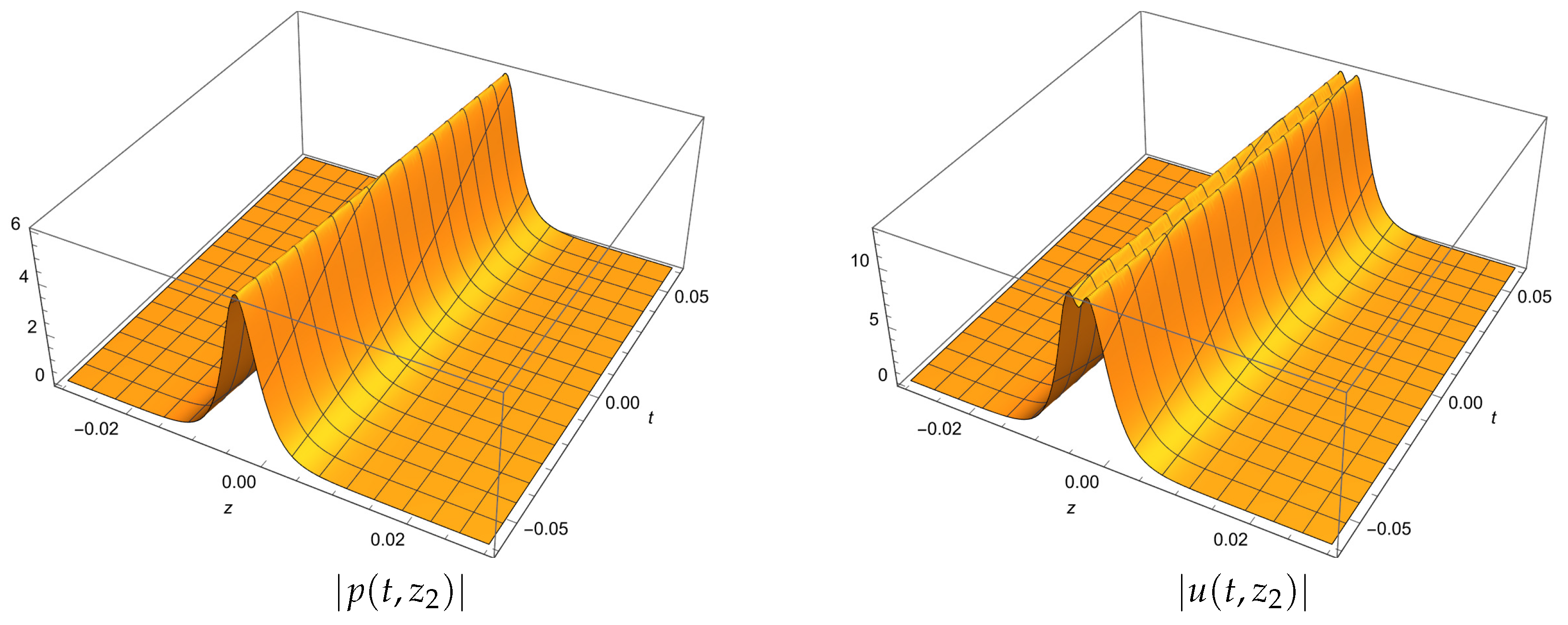
Figure 1.
The amplitudes of the solution (35) for , .
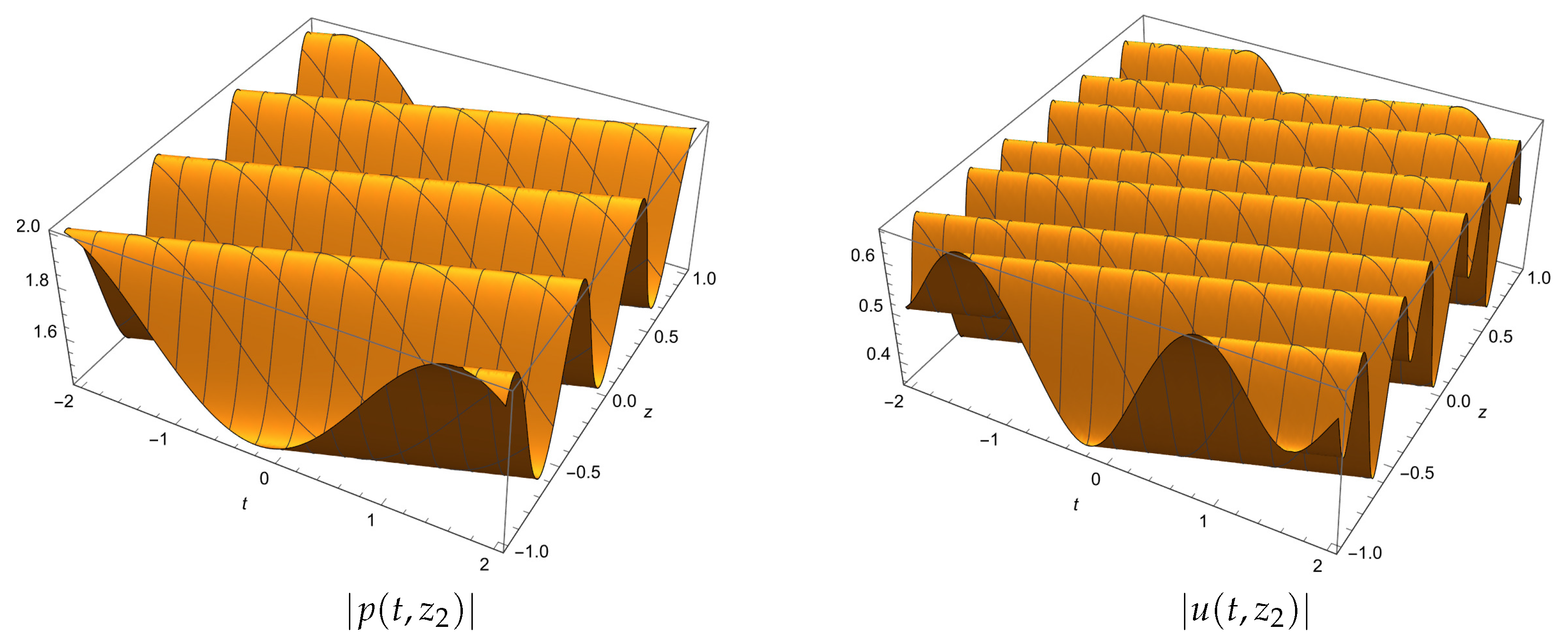
Figure 2.
The amplitudes of the solution (38) for , .
Disclaimer/Publisher’s Note: The statements, opinions and data contained in all publications are solely those of the individual author(s) and contributor(s) and not of MDPI and/or the editor(s). MDPI and/or the editor(s) disclaim responsibility for any injury to people or property resulting from any ideas, methods, instructions or products referred to in the content. |
© 2023 by the authors. Licensee MDPI, Basel, Switzerland. This article is an open access article distributed under the terms and conditions of the Creative Commons Attribution (CC BY) license (http://creativecommons.org/licenses/by/4.0/).
Copyright: This open access article is published under a Creative Commons CC BY 4.0 license, which permit the free download, distribution, and reuse, provided that the author and preprint are cited in any reuse.


