
Submitted:
07 August 2025
Posted:
08 August 2025
You are already at the latest version
Abstract
Accurate forecasting of solar power generation is becoming increasingly important in the context of renewable energy integration and intelligent energy management. The variability of solar radiation, caused by changing meteorological conditions and diurnal cycles, complicates the planning and control of photovoltaic systems and may lead to imbalances in supply and demand. This study aims to identify the most effective exponential smoothing approach for real-world PV generation forecasting using actual hourly generation data from a 9 MW solar power plant in the Kyiv region, Ukraine. Four exponential smoothing techniques are analysed: Classic, a Modified сlassic adapted to daily generation patterns, Holt’s linear trend method, and the Holt-Winters seasonal method. The models were implemented in Microsoft Excel using real measurement data collected over six months. Forecasts were generated one hour ahead, and optimal smoothing constants were identified via RMSE minimisation using the built-in Solver tool. Substantial differences in forecasting accuracy were observed. The Classic simple exponential smoothing model performed worst, with an RMSE of 1413.58 kW and nMAE of 9.22%. Holt’s method improved trend responsiveness (RMSE = 1052.79 kW, nMAE = 5.96%), but still lacked seasonality modelling. Holt-Winters, which incorporates both trend and seasonality, achieved a strong balance (RMSE = 1031.00 kW, nMAE = 3.7%). The best performance was observed with the Modified simple exponential smoothing method, which captured the daily cycle more effectively (RMSE = 166.45 kW, nMAE = 0.84%). The study identifies forecasting models that combine accuracy with low computational complexity, making them suitable for lightweight real-time energy control systems. The Modified simple exponential smoothing model, in particular, offers a high degree of precision and interpretability, supporting its integration into operational PV forecasting tools.
Keywords:
solar power forecasting
; exponential smoothing
; Holt method
; Holt-Winters method
; PV generation
; time series forecasting
; sequential data models
1. Introduction
Photovoltaic (PV) generation has become a cornerstone of global efforts to decarbonise the energy sector. In recent years, many countries have significantly expanded their installed PV capacity as part of broader strategies to reduce greenhouse gas emissions and enhance energy security. As the share of solar energy in the electricity mix increases, its inherent variability and intermittency pose operational challenges for power systems. In this context, accurate short-term forecasting of solar power output is essential for maintaining Grid stability, enabling demand-supply balancing, scheduling backup resources, and optimising energy storage systems. Moreover, national energy-consumption forecasting under wartime conditions has been studied for Ukraine, illustrating the need for robust and adaptable forecasting models in crisis scenarios [1].
In [2,3], the authors emphasise the increasing role of micropower systems based on renewable energy sources in enhancing the resilience of modern PowerGrids through distributed generation, storage, and intelligent control. Moreover, intelligent MPPT strategies such as self-tuning fuzzy logic controllers have been developed to optimise PV energy extraction and enhance operational reliability in grid-connected hybrid renewable energy systems [4]. In a related study [5], a mathematical energy balance model was presented for the Smila community in Ukraine, showing that increasing the renewable share from 55% to 69%, while simultaneously reducing electricity imports by 30%, led to a 3.5-fold reduction in CO₂ emissions. The study underlined the practical importance of forecasting models that align renewable energy generation with daily load fluctuations in decentralised energy systems.
Solar irradiance is a key factor influencing PV output – the intensity of solar irradiation reaching photovoltaic panels [6]. While many forecasting approaches directly model irradiance as an intermediate step [7,8], this study focuses on forecasting the PV power output. Framing the task as a time series prediction problem allows for direct integration into operational energy management systems without requiring explicit irradiance modelling. This approach addresses the need for efficient and scalable solutions for Grid-responsive control.
Various approaches have been proposed for short-term forecasting of solar generation, including numerical weather prediction, hybrid machine learning techniques, and statistical time series models [9,10,11,12]. However, in many practical settings – particularly those constrained by limited data, hardware resources, or deployment time – statistical models remain a highly relevant alternative.
The growing integration of PV systems into power grids has significantly increased the importance of accurate solar power forecasting. As grid-connected PV capacity expands, particularly in regions where solar penetration exceeds 20%, the economic and operational consequences of forecast errors become more pronounced. Balancing costs linked to solar variability can account for up to 15% of total system dispatch expenditures, emphasizing the need for more precise and responsive forecasting methodologies [13,14,15,16,17].
Ultra-short-term forecasting of PV output presents distinct challenges, especially in capturing rapid fluctuations caused by transient cloud cover and atmospheric disturbances. These phenomena can induce power swings of several hundred kilowatts within minutes, directly affecting grid stability and reserve allocation strategies [18,19].
Recent studies have demonstrated that the integration of sky-camera imagery and advanced textural convolution techniques can reduce forecasting errors during cloudy conditions by up to 30%, highlighting the value of visual data in enhancing real-time prediction accuracy [18,19,20].
Advancements in deep learning have led to the development of hybrid models that combine convolutional neural networks (CNNs) for spatial feature extraction with long short-term memory (LSTM) networks for temporal sequence modeling. These architectures have shown superior performance over traditional statistical methods when applied to non-linear and intermittent PV datasets [21,22,23].
In particular, time–frequency domain approaches that incorporate wavelet decomposition alongside LSTM structures have achieved normalized RMSE reductions exceeding 25% compared to standalone exponential smoothing models [22,24]. Additionally, transfer learning frameworks based on foundation models have demonstrated promising results in zero-shot forecasting for newly commissioned PV installations, with accuracy improvements reaching 70% in early-stage deployments [25].
From an operational standpoint, forecasting models must balance accuracy with computational efficiency and interpretability. Implementations on edge-computing platforms have shown that hybrid statistical and machine learning ensembles can meet sub-minute update requirements using modest hardware resources, supporting both centralized grid operations and local energy management systems [14,15,16,17].
The use of auxiliary data sources—such as satellite-derived irradiance and all-sky imaging—further strengthens model robustness under variable meteorological conditions. These multimodal approaches reflect a broader shift toward domain-aware forecasting frameworks that are well-suited to the evolving demands of solar energy integration [18,19,20,26].
While advanced machine learning techniques continue to push the boundaries of forecasting accuracy, their complexity and resource demands often limit their applicability in embedded or real-time control environments. In many operational contexts—particularly those constrained by hardware limitations, deployment speed, or the need for model interpretability—statistical methods remain indispensable. Among these, exponential smoothing techniques have retained their relevance due to their simplicity, transparency, and adaptability to high-frequency data streams [27].
A comprehensive review [28] emphasised the continued relevance of exponential smoothing methods in forecasting applications where computational efficiency and transparency are paramount. The study identified simple exponential smoothing (SES), Holt’s linear method, and Holt-Winters’ seasonal method as competitive options under stable operational conditions, especially for embedded or resource-constrained systems. Similarly, [29] categorised exponential smoothing as a core family of statistical methods suitable for rapid deployment in real-time grid environments. These models remain widely used in forecasting both load and generation, particularly where high-frequency data and fast forecast updates are required.
Exponential smoothing methods generate forecasts as weighted averages of past observations, with more recent values given higher weight. Depending on the structure of the underlying data, different model variants are applicable: SES for level prediction, Holt’s method for linear trends, and Holt-Winters for seasonal time series. These models have been successfully applied across a wide range of energy forecasting tasks, including electricity consumption, wind energy output, and PV generation.
In [30], authors validated the practical value of exponential smoothing techniques, particularly the Holt-Winters method, in short-term load forecasting under variable socio-economic conditions. Their study compared the performance of Holt-Winters and Prophet algorithms for forecasting hourly electricity demand in Houston, Texas, during the COVID-19 pandemic. Despite the simplicity of the Holt-Winters approach, the authors demonstrated its robustness and reliability across multiple intra-day forecasting intervals. While Prophet provided marginally better generalisation, Holt-Winters was praised for its simplicity and ease of implementation, especially in embedded control systems. Furthermore, study [31] extended the application of exponential smoothing to probabilistic forecasting in the Australian National Electricity Market, using it to construct prediction intervals for solar and wind generation. The study demonstrated that exponential smoothing could match or exceed the performance of more complex approaches, such as quantile regression and ARCH/GARCH models, in generating reliable confidence bounds for renewable generation.
Although exponential smoothing methods may lack the sophistication of deep learning algorithms, they remain competitive in many practical contexts, particularly when forecasting performance must be balanced against implementation constraints. Their inherent interpretability and ability to respond to dynamic trends make them an attractive choice for real-time energy forecasting in operational environments.
The goal of the paper is to conduct a comparative analysis of four exponential smoothing techniques for PV generation forecasting – the Classic SES model, a modified SES approach adapted to capture diurnal patterns, Holt’s linear trend method, and the Holt–Winters seasonal method – and to evaluate their forecasting accuracy using actual hourly generation data, ultimately identifying the most effective approach for lightweight, accurate, and interpretable real-world PV forecasting applications.
2. Data Description
This study utilised real-world data obtained from a ground-mounted photovoltaic power plant (PVPP) located in Velyka Dymerka, Kyiv region, Ukraine. The facility has an installed capacity of approximately 9 MW and operates in a Grid-connected configuration. The dataset comprises active power output measurements recorded at 10-minute intervals over a continuous seven-month period, from January 1 to July 1, 2021.
Given the high temporal resolution and large volume of the raw data, a normalisation step was applied by aggregating the 10-minute measurements into hourly averages. This transformation reduced the dimensionality of the dataset while preserving essential temporal characteristics, facilitating analysis and aligning with the operational requirements of energy management systems. For each hour h, the average active power output was computed as:
where denotes the average PVPP power outputs for hour h, represents the PVPP power output measured at the i-th 10-minute interval within hour h, i is the index of the six 10-minute intervals in each hour.
The resulting time series captures both intra-day (diurnal) and inter-day (seasonal) variability typical of PV systems in mid-latitude regions. Due to the solar cycle and geographic location, the PVPP exhibited zero or near-zero generation during nighttime hours, typically spanning approximately six hours per day, resulting in nearly half of the dataset containing zero values. These periods of inactivity alternate with clear and sharply defined daytime generation profiles, as illustrated in Figure 1 and Figure 2.
Figure 1 illustrates the hourly PVPP power output for three representative months – January (a), April (b), and July (c) – based on the cleaned and aggregated dataset. This comparison highlights the pronounced temporal variability and seasonal characteristics of PV generation. In January, the PV system generates low and irregular energy outputs, with many days displaying near-zero generation. Short daylight hours and frequent winter cloud cover contribute to the limited generation. Peak values rarely exceed 5,500 kW, and daily profiles are sparse and inconsistent, highlighting the challenge of forecasting under winter conditions. By April, the generation profile becomes more defined and stable. The days are longer, and daily peak outputs frequently range between 6,000 and 8,000 kW. The curves exhibit greater consistency, reflecting improved insolation and fewer weather-related disruptions. The typical bell-shaped diurnal patterns begin to emerge, signifying a seasonal shift toward more predictable generation. In July, the PV output reaches its highest levels and greatest regularity. The plant operates close to its nominal capacity, with many days showing smooth, symmetric diurnal curves. The hourly peaks are consistently above 8,000 kW, with minimal variability from day to day. This stability reflects optimal solar irradiance and clear-sky conditions characteristic of midsummer.
Figure 1.
Hourly PV power generation: a) January, b) April, c) July.
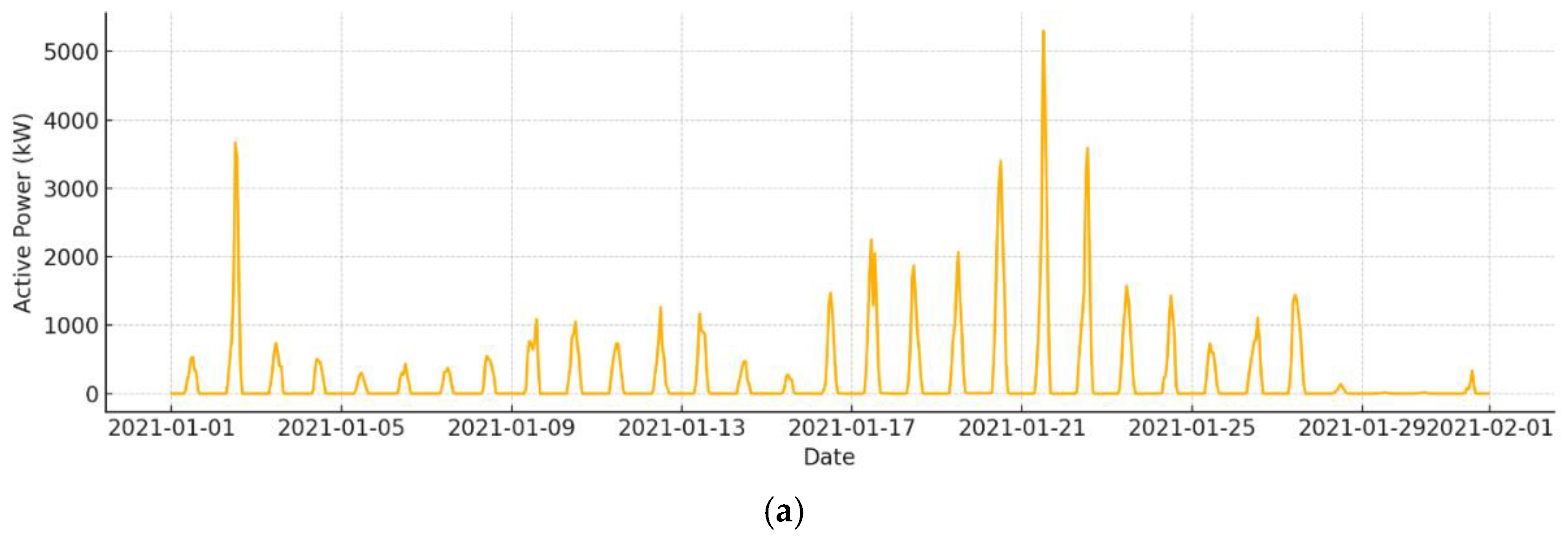
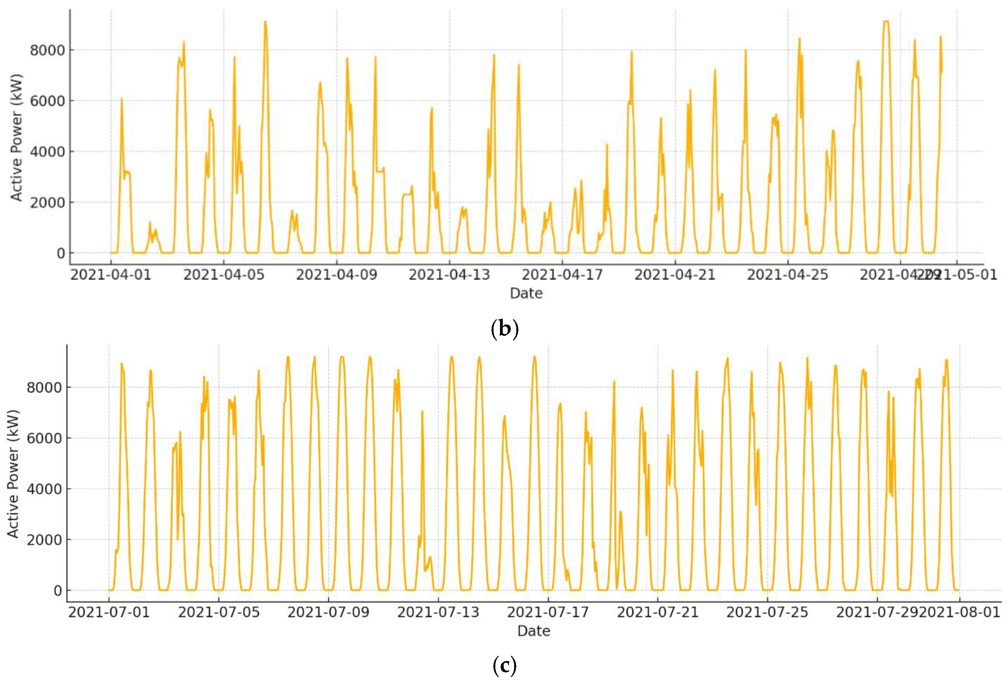
Figure 2.
Comparative hourly PV generation for selected months.
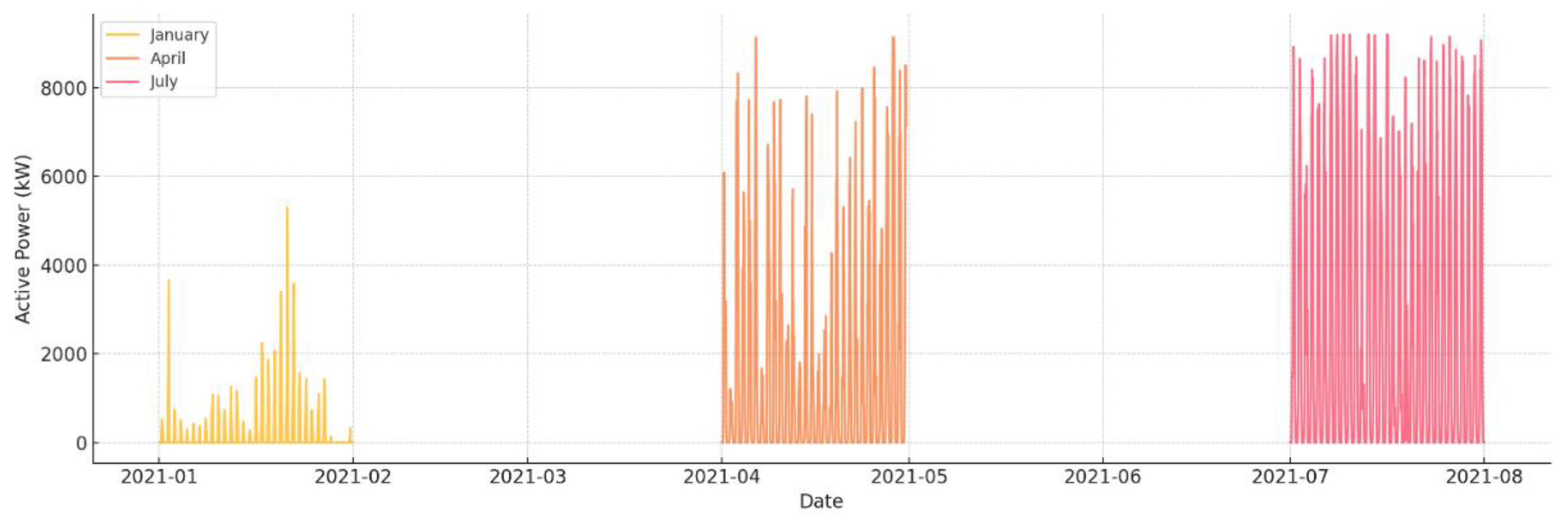
Figure 2 offers a comparative view of the same months as Figure 1, but with data overlaid on a single plot. The overlapping curves highlight the monthly differences in both magnitude and duration of daily generation. This representation reinforces the visual understanding of seasonal amplitude shifts and underlines the importance of capturing both intra-day structure and inter-month transitions in forecasting models.
Together, these graphs demonstrate a clear evolution from low, variable winter output to high, stable summer generation. The seasonal pattern emphasises the importance of capturing trend and seasonality in forecasting models. Given the observed regularity and structure in the summer months and the noisier, intermittent behaviour in winter, the time series is well-suited for exponential smoothing methods that can adapt to both persistent trends and recurring diurnal cycles.
Figure 3 presents the average daily PV generation profiles by hour of day for each month from January to July. Each curve represents the mean hourly active power output aggregated over all days within the corresponding month. This figure highlights the distinct diurnal nature of solar generation and its seasonal modulation in both intensity and duration.
Figure 3.
Average daily PV generation profiles averaged over all days within each month.
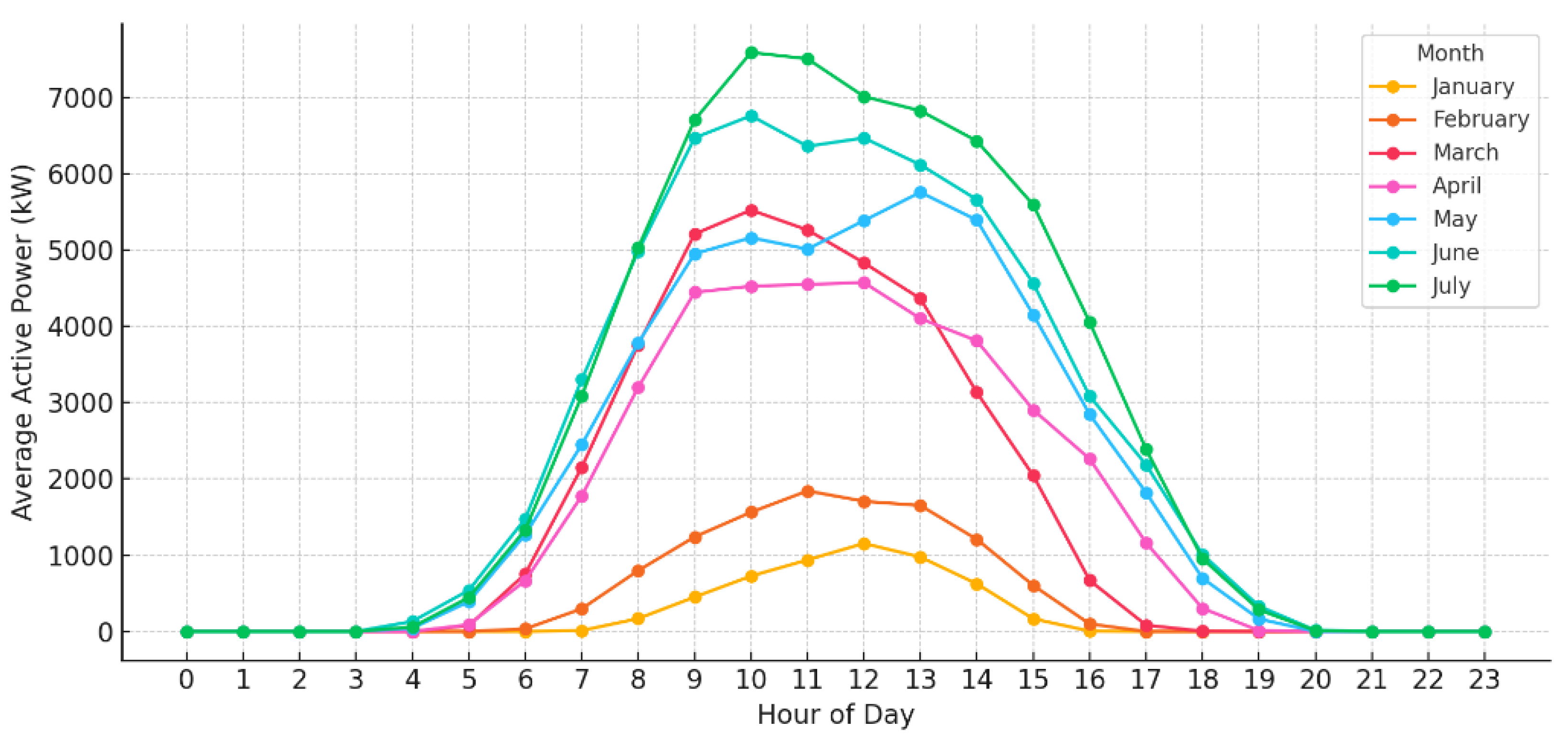
Across all months, the generation profile follows a consistent unimodal shape, with zero production during the night, followed by a rapid rise in the early morning, a peak around solar noon, and a gradual decline towards evening. However, the shape and magnitude of these profiles vary significantly by season. In the winter months (January and February), generation is constrained to a narrow time window between approximately 8:00 and 16:00, with modest peak values not exceeding 2,000 kW. This limited output reflects the combination of short daylight periods, low solar elevation angles, and potentially frequent cloud cover. March and April show notable increases in both the peak power and the width of the daily curve, indicating longer days and improved irradiance conditions. The generation window extends from roughly 7:00 to 18:00, with peak values ranging between 4,000 and 6,000 kW. By late spring and early summer (May to July), the generation profile becomes broader and more symmetric, with the earliest onset and latest cutoff of production. In these months, peak output frequently exceeds 7,000 kW, and the system remains at high generation levels for several consecutive hours around midday. These months correspond to the most favourable solar conditions, characterised by high irradiance and minimal atmospheric interference.
The evolution of the curves in Figure 3 demonstrates both intra-day regularity and inter-month variability of PV output. The pronounced seasonal shift in the height and width of the profiles underscores the necessity of incorporating both trend and seasonality into forecasting models.
Figure 4 visualizes the evolution of daily average PV power output throughout the observation period, highlighting both the seasonal trajectory and the variability in daily generation within each month. Unlike aggregated hourly profiles (Figure 3), this representation captures the net energy yield of each day, revealing how short-term fluctuations and broader climatic trends shape PV system performance.
In the early months (January and February), daily generation values are generally low, and the curve is characterised by high irregularity. Sharp transitions between near-zero and moderate-output days suggest a strong influence of atmospheric variability, such as passing clouds or snowfall, which can significantly diminish irradiance under already constrained winter conditions. Notably, some days achieve brief peaks around 1,000 kW, but these are interspersed with extended periods of negligible production. As advancing into spring (March and April), the Fig. reveals a dual effect: an upward shift in the baseline generation and a reduction in volatility. This period marks the transition from erratic to more sustained power output, reflecting longer daylight hours and a gradual stabilisation of weather patterns. However, periodic declines remain visible, underscoring the persistence of intermittent meteorological disruptions.
Figure 4.
Daily average PV generation over the year, grouped by month.
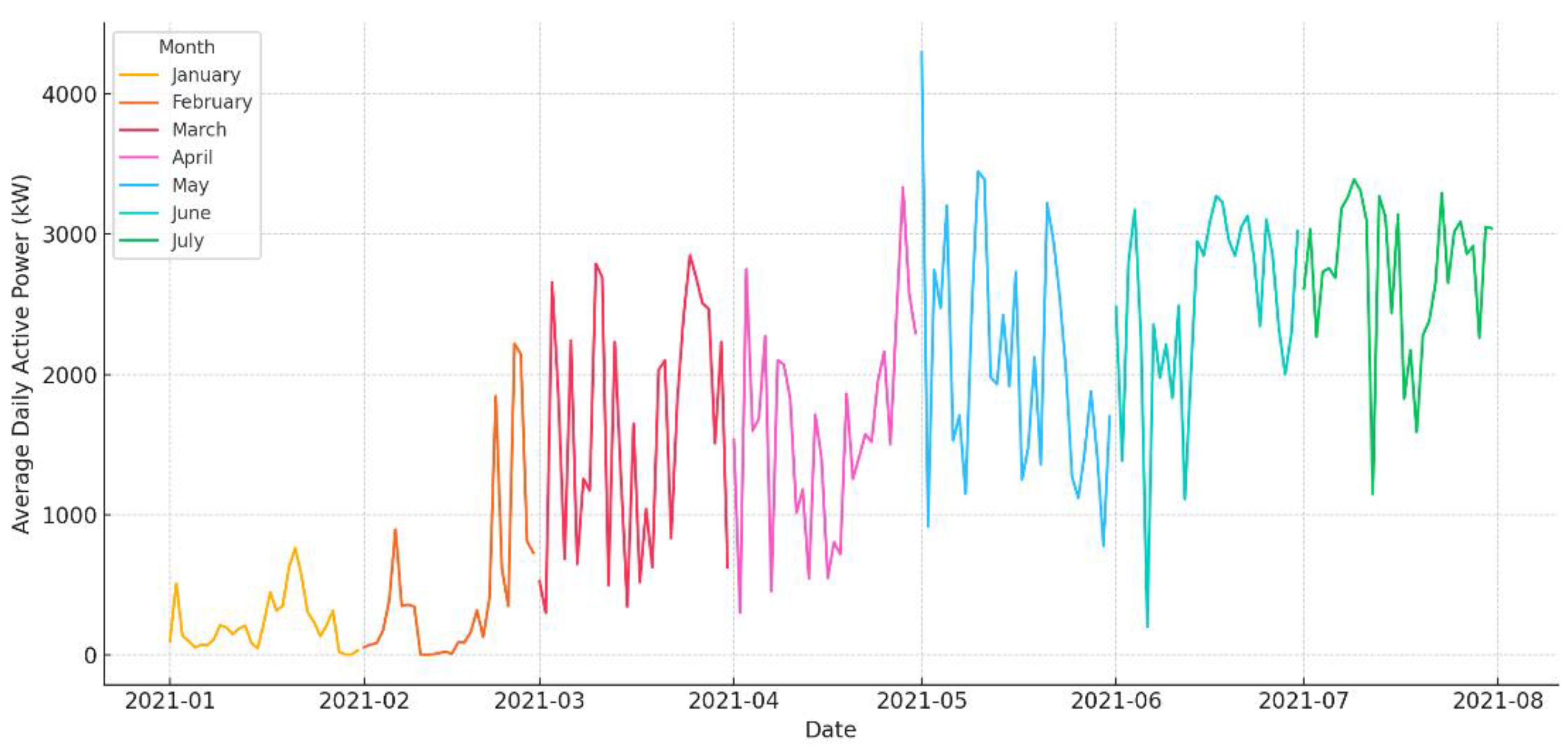
The most stable and elevated performance is evident from May onward. Both June and July display tightly clustered data points in the upper range of the vertical axis, with daily averages frequently exceeding 3,000 kW. This concentration suggests favourable and consistent solar conditions over prolonged intervals, allowing the PVPP to operate near its design capacity. Yet, even in these peak months, a few outliers indicate the influence of localised weather events or transient shading.
What makes this visualisation particularly valuable is its capacity to reflect inter-day reliability and generation continuity – metrics that are crucial for energy planning, especially in systems with high PV penetration. The gradual flattening of fluctuations from winter to summer demonstrates the increasing predictability of solar output, which has direct implications for forecast model training, resource allocation, and grid integration strategies.
In summary, Figure 4 provides evidence of a strong seasonal signal coupled with diminishing short-term variability over time. It supports the conclusion that forecasting models must be capable not only of modelling trends and seasonality but also of responding to non-systematic deviations in daily energy yield caused by short-lived weather events.
3. Data Preprocessing
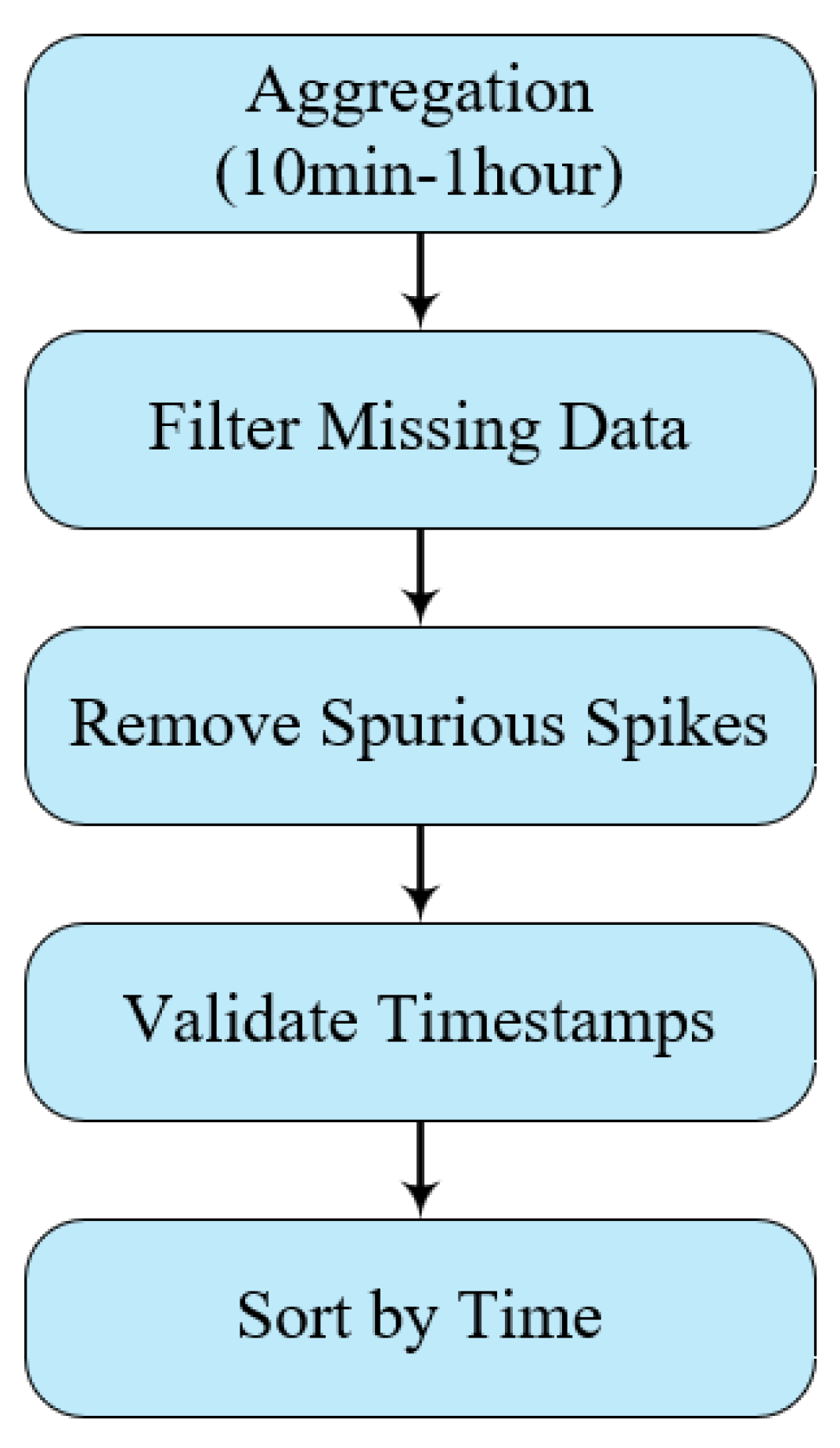
Before applying forecasting methods, the raw dataset was subjected to a comprehensive preprocessing procedure to ensure data quality, temporal consistency, and suitability for time series analysis. A visual overview of the preprocessing workflow is presented in Figure 5.
The diagram illustrates the sequential steps applied to clean and prepare the PV time series data before forecasting, including covering aggregation, anomaly removal, timestamp validation, and sorting.
The original time series, recorded at 10-minute intervals, was first aggregated into hourly averages. This step reduced the dimensionality and retained the essential temporal dynamics relevant to PV generation.
The preprocessing workflow included several key steps. Missing or incomplete records were identified and removed to eliminate discontinuities. Spurious spikes in active power output – typically caused by the sensor noise, inverter fluctuations, or communication errors – were detected through visual inspection and filtered using empirically defined upper bounds based on system performance. Additionally, the dataset was examined for duplicate entries and inconsistent time stamps, which were corrected to maintain uniform hourly intervals and strict chronological order.
Unlike in machine learning tasks involving gradient-based optimisation or neural networks, normalisation was not applied in this study. The exponential smoothing methods used in this analysis – such as simple, double, and triple smoothing – are scale-independent and operate directly on the raw magnitudes of the time series. Normalisation could reduce interpretability in the context of physical units (e.g., kW) and was therefore intentionally avoided to maintain the clarity and traceability of forecasted values in real operational terms.
Figure 5.
Data preprocessing scheme.
To reconstruct short, isolated missing values that remained after initial filtering, linear interpolation was applied at the final stage of preprocessing. This method estimates a missing value based on its nearest valid neighbours in time. In this context, the horizontal axis t represents time (in hours), and the vertical axis P denotes the active power output. The interpolated value P(t) was estimated using the Equation (2):
where P(t) is the interpolated power at time t, and (t1, P1), (t2, P2) are the nearest valid observations before and after the missing time point.
Since only five values were missing across the entire dataset, the overall share of missing data was statistically negligible. This further justified the use of a simple and transparent interpolation method over more complex approaches. Linear interpolation was therefore selected for its robustness, interpretability, and adequacy in restoring isolated gaps without distorting the overall signal dynamics. Given the hourly resolution and the small proportion of missing values, this method was considered both efficient and sufficiently accurate.
As a result, a clean and consistent dataset was obtained, accurately reflecting both intra-day and seasonal dynamics in PV output.
4. Forecasting Models
4.1. Simple Exponential Smoothing (SES) Method
SES is a widely used forecasting method suitable for time series data that fluctuates around a relatively constant mean, without trend or seasonal effects. It is particularly effective in short-term forecasting tasks where the underlying process is stable or changes gradually.
SES generates forecasts by applying exponentially decreasing weights to past observations, with the most recent data having the strongest influence on the forecast. The fundamental idea is that older data points carry less information about the future, and their impact should decay over time.
The basic SES formula is given by the Equation (3) [32]:
where is the forecasted power at time , is the actual observed value at time t, is the forecast made for time t, is the smoothing constant controlling the weighting.
This decay mechanism enables the method to respond to recent changes while maintaining stability in the presence of noise. A low α value results in strong smoothing, making the model slow to respond to changes, while a high α value increases sensitivity to recent fluctuations.
In the context of PV generation, SES is best applied under conditions of stable irradiance, such as clear-sky days with minimal meteorological variability. However, it cannot capture long-term upward or downward trends or seasonality, which are typical in PV generation due to diurnal and annual cycles.
From a comparative evaluation standpoint, [33] demonstrated that SES performed well in terms of execution time and basic accuracy metrics (RMSE, MAE), especially under low-complexity scenarios. However, its predictive power diminished in the presence of structural trends, as evidenced by negligible or undefined R2 values and zero correlation in datasets with large variability. Similarly, [34] emphasised that the performance of SES strongly depends on the proper selection of the smoothing constant α. This parameter is typically optimised by minimising error metrics. For instance, their study showed that α values in the range of 0.26-0.29 yielded excellent accuracy (MAPE < 10%) when forecasting electricity production data.
Its comparative simplicity and interpretability make it a useful benchmark, especially in systems where computational constraints are present or model transparency is required.
4.2. Modified Simple Exponential Smoothing Method
While Classic SES provides a baseline approach for time series forecasting without trend or seasonality, it may not adequately reflect the repetitive daily patterns observed in PV generation. To address this, a modified version of SES is proposed by the authors, designed specifically for PV output prediction by incorporating historical data from previous days for the same hour.
This modification extends the SES framework by averaging actual or forecasted values from the same hour of the previous day, thus embedding diurnal structure directly into the forecast. The modification is particularly suitable for time series exhibiting strong daily regularity but limited long-term trend, as in the case of hourly PV generation under relatively stable weather conditions.
The method forecasts the active power output P at a given hour h and day d by incorporating the actual or previously forecasted value from the same hour on the preceding day. The updated smoothing equation is defined as:
where is the forecasted power for day d and hour h, is the actual observed power at the same time, is the forecasted power for the previous day at the same hour, is the smoothing constant controlling the influence of recent values.
This structure preserves the simplicity of the original SES model while enhancing its temporal consistency by embedding knowledge of recurrent daily cycles. It improves adaptability to short-term fluctuations in solar irradiance due to transient weather conditions, while remaining computationally efficient and interpretable.
The proposed modification is especially beneficial when actual measurements are delayed or unavailable, as it allows forecasts to rely on previous estimations without disrupting continuity. The method maintains a balance between accuracy and efficiency, making it well-suited for deployment in local energy management systems or real-time control environments.
4.3. Holt`s Exponential Smoothing Method
Holt’s exponential smoothing method extends the сlassic SES approach by explicitly incorporating a trend component. This allows the model to forecast time series that exhibit a systematic increase or decrease over time, behaviour frequently observed in PV generation due to gradually changing irradiance during the day or seasonal transitions.
The method maintains two recursive components:
- Level (Lt): captures the smoothed value of the series at the current time.
- Trend (Tt): estimates the rate of change from one time step to the next.
The power output forecast for k time steps ahead is computed as [35]:
where Lt is the smoothed level component at time t, Tt is the trend estimate at time t, is the forecast for k hours ahead, are smoothing constants for the level and trend components, respectively.
In the context of PV forecasting, Holt’s method is particularly effective in capturing intra-day ramp-up in the morning and ramp-down in the evening, especially on clear-sky days. It is also useful during transitional months such as early spring or late summer, when solar altitude changes produce gradual variations in hourly power output. Unlike SES, which assumes a stationary mean, Holt’s method dynamically adapts to persistent changes in power generation. This makes it more suitable for periods with a systematic trend in solar irradiance. However, its inability to model repetitive intra-day patterns limits its performance during months characterised by strong daily seasonality.
From a practical standpoint, Holt’s method offers favourable computational efficiency. This is crucial for real-time applications or deployment on embedded systems. Still, the quality of predictions heavily depends on the appropriate tuning of α and β. These parameters control the model’s responsiveness to recent changes – higher values enable faster adaptation, while lower values yield smoother, more stable trend estimations.
A recent study [36] successfully applied Holt’s method to model mid-term trends in Ukraine’s renewable energy deployment. Their results demonstrated that the method effectively captured upward capacity growth trajectories for wind, solar, and biomass energy. This evidence supports Holt’s model as a viable tool not only for time series forecasting but also for energy sector planning and scenario development.
In summary, Holt’s exponential smoothing method offers a balanced approach between adaptability and simplicity. Its ability to handle non-stationarity without introducing excessive complexity makes it a strong candidate for forecasting PV generation under conditions of evolving irradiance but lacking regular cyclic patterns.
4.4. Holt-Winters Exponential Smoothing Method
The Holt-Winters exponential smoothing method extends Holt’s trend-corrected model by adding a third component – seasonality. This enhancement makes the method particularly suitable for forecasting time series that exhibit both trend and recurring seasonal patterns, such as those observed in PV generation.
There are two common variants of Holt-Winters: additive and multiplicative.
The model decomposes the series into three components:
- Level (Lt) is the smoothed estimate of the central tendency.
- Trend (Tt) is the smoothed estimate of the slope.
- Seasonality (St): the cyclic pattern repeating every s periods (e.g., daily).
The additive Holt-Winters model is defined by the following recursive equations (8-11) [37]:
where s is the seasonality length (e.g., 24 for hourly data with daily cycles), k is the forecast horizon, are smoothing constants for level, trend, and seasonality, respectively.
These formulations allow the model to adapt to fluctuations caused by meteorological variability, changes in solar angles, and the daily cycle of irradiance. The seasonal component plays a crucial role in capturing the regular, diurnal rhythm of PV output, where solar power generation rises and falls predictably with the sun’s position.
The method has seen widespread application in both academia and industry. For instance, [34] demonstrated its effectiveness in modelling electricity demand patterns exhibiting strong weekly and monthly cycles. Similarly, in [30] was employed the Holt-Winters method for intra-day load forecasting during the COVID-19 pandemic, showing that it maintained stable performance under volatile conditions. Their findings indicated that the additive model provided more consistent results than ARIMA and LSTM under normal weather conditions, while offering the benefits of lower computational demand and easier interpretability.
Although Holt-Winters is computationally more demanding than SES or Holt’s linear trend model, it remains lightweight compared to machine learning techniques. At the same time, it offers full transparency regarding the contribution of each component to the forecast.
4.5. Metric for Model Performance Evaluation
To evaluate the forecasting performance of the exponential smoothing methods, the following statistical metrics are employed: the coefficient of determination (R²) (16), rootmean square error (RMSE) (17), normalised RMSE (nRMSE) (18), mean absolute error (MAE) (19), and normalised MAE (nMAE) (20):
where are the actual power values, are the corresponding estimated values, is the mean of measured power data points, and is the number of measurements.
In contrast to RMSE, which is influenced by the absolute values of measured power, the normalised RMSE (nRMSE) serves as a scale-independent indicator of forecasting accuracy for power output. This metric evaluates the consistency between predicted and actual power values, with an nRMSE of 100% representing perfect predictive alignment. Lower nRMSE values reflect diminished forecasting precision.
Similarly, the normalised MAE (nMAE) complements nRMSE by expressing the average magnitude of forecasting errors relative to the range of the measured data. While RMSE penalises larger deviations more severely, nMAE provides a more interpretable, absolute measure of average forecast deviation. This metric is particularly useful in comparing model accuracy across systems with different scales of generation. Lower nMAE values indicate improved alignment between forecasted and observed values, especially during periods with moderate or steady production.
Together, reduced RMSE and MAE values, combined with R² values approaching 1, indicate stronger agreement between the predicted and actual power output and thus improved model accuracy in PV generation forecasting.
5. Results and Discussion
This section compares the predictive performance of each method based on performance metrics, discusses the influence of model structure and parameter selection, and highlights the strengths and limitations of each approach. Special attention is given to the proposed modification of the SES model, which integrates diurnal characteristics of solar generation and is evaluated against the baseline and more complex smoothing methods.
For each model, forecasting was conducted on a cleaned and preprocessed hourly time series representing active power generation from a 9 MW PV plant. All models were applied in a rolling window manner, with parameters optimised on a validation subset of the data.
For Classic SES and Modified SES, the smoothing constant α was tuned within the range [0.0; 1.0] using step-wise search, selecting the value minimising RMSE on the validation portion.
Holt’s model involved simultaneous tuning of α and β (level and trend), while the Holt-Winters method additionally required optimisation of γ (seasonality). The seasonal period was set to 24 hours to match the daily PV generation cycle.
No data normalisation was applied to preserve the interpretability of the power values in kilowatts.
The forecasting horizon was one hour ahead, with each model generating point forecasts based on preceding data only. Forecasting was carried out entirely in Microsoft Excel, leveraging its built-in functionality for transparent and reproducible analysis. For each model, the optimal smoothing constants – such as α for SES and Modified SES, and α, β, and γ for Holt and Holt-Winters – were determined using the Excel Solver tool. The objective function was set to minimise RMSE on a validation subset of the data. This approach allowed for intuitive implementation, facilitated parameter tuning without requiring external software, and ensured the consistency and repeatability of the modelling process. As emphasised in [39], selecting an appropriate smoothing constant α is critical for achieving accurate forecasts using the SES method. Their study demonstrated that optimising α through mean squared error minimisation notably improves prediction performance. While their application focused on supply chain forecasting, the principles are equally valid for energy systems with repetitive temporal structures, such as PV generation. This supports the current study’s choice to calibrate α using Excel Solver for each model to minimise RMSE across the validation subset, ensuring tailored responsiveness to the unique dynamics of solar power output.
The Classic Simple Exponential Smoothing method was evaluated across a wide range of smoothing constant, , in increments of 0.1, to analyse the model’s sensitivity and performance at different responsiveness levels. Forecasts were generated for each α value using the cleaned and aggregated hourly PV power dataset.
Each SES variant used only the previous actual value and the last forecast to compute the next prediction. The model’s simplicity allows it to react to recent changes in data, with the degree of responsiveness governed by the smoothing parameter α.
The performance of each α configuration was visually assessed using plotted forecast profiles and numerically evaluated by calculating RMSE on the validation subset. The optimal value of α was selected based on the configuration that minimised the RMSE, balancing short-term reactivity with noise suppression.
Despite its interpretability and computational simplicity, SES was limited in accurately forecasting the PV time series due to its inability to capture recurring patterns such as daily seasonality or long-term trends. These structural limitations led to notable errors, particularly during transitions between low and high irradiance periods.
The methodological foundation of the Modified SES model proposed in this study is rooted in the need to enhance the responsiveness of SES to the recurring diurnal patterns typical of PV generation. Unlike the Classic SES, which bases its forecast exclusively on the previous value and forecast, the modified version integrates the actual value observed at the same hour on the previous day. This structure directly captures the cyclic behaviour of solar energy generation, where daily irradiance patterns strongly influence output.
The forecasting procedure was executed using a cleaned and hourly-aggregated PV power dataset. For each hour, forecasts were generated using the prior day’s actual value at the same hour, combined with the exponential smoothing forecast of that hour. α was evaluated in 0.1 increments between 0.0 and 1.0, with RMSE computed on a validation subset to identify the optimal configuration.
This approach demonstrated a remarkable capacity to balance responsiveness and stability, particularly around transition periods (sunrise/sunset), while preserving computational simplicity. Forecast accuracy improved dramatically compared to the classic SES, and the model proved especially robust during high-variability periods such as partial cloudiness or shifting irradiance conditions.
A similar conceptual framework was explored in [40], which proposed two SES-based models for solar irradiance and load forecasting in hybrid energy systems. Their second model, which also used same-hour values from the previous day, resembles our modification. However, there are key methodological differences. Lim and Nayar implemented their models on synthetic irradiance data generated in the HOMER simulation platform, without evaluation on real-world PV generation data. Additionally, they did not optimise α using an RMSE-based criterion, nor did they perform a comprehensive grid search over multiple α values. Their analysis, though innovative for its time, lacked empirical validation against actual PV output, and the model’s performance was not benchmarked using standard error metrics across multiple scenarios.
In contrast, the present study’s Modified SES model was rigorously tested using real operational data and systematically optimised for forecasting accuracy. The use of actual plant data from Ukraine and careful calibration of smoothing parameters makes this implementation not only more reliable but also more applicable for real-world energy forecasting.
While the conceptual foundation, in [40], validates the efficacy of integrating prior-day data, the methodological rigour, empirical validation, and performance benchmarking of our Modified SES model demonstrate a superior and more practical solution.
Holt’s method extends the Classic SES by introducing a second equation to explicitly model the trend component of the time series. This makes it particularly suitable for capturing gradual increases or decreases in solar generation over time, which often arise due to changing cloud cover, sunrise/sunset transitions, or seasonal shifts in solar angles.
For each pair (α, β), forecasts were generated iteratively across a validation subset, and the corresponding RMSE was calculated.
Visual inspection of forecast profiles confirmed that Holt’s method successfully captured medium-term linear trends in the PV generation data, such as ramp-up and ramp-down periods during morning and evening hours. However, the method exhibited limitations in modelling recurring diurnal cycles and abrupt changes in irradiance, resulting in reduced accuracy compared to models with seasonal components.
While Holt’s method provided a significant improvement over Classic SES by accommodating trend dynamics, its inability to model seasonality directly limited its performance. Nevertheless, the model remains valuable for forecasting in contexts where linear trends dominate or computational simplicity is a priority.
Next, the Holt-Winters method was investigated as a natural extension, offering both trend and seasonal components. To ensure optimal performance, both the additive and multiplicative forms were compared, aiming to identify which better aligns with the seasonal dynamics of hourly PV output. As previously shown in Figure 1, the active power time series exhibits strong daily seasonality, with a notable variation in seasonal amplitude. The winter months are characterised by lower daily peaks, while the summer months show higher and broader daily fluctuations. This behaviour is consistent with the physical nature of solar irradiance, which changes seasonally due to astronomical and meteorological factors. To verify the type of seasonality, seasonal decomposition of the time series was performed using both additive and multiplicative models. The decomposition results are presented in Figure 6 and Figure 7, respectively.
Figure 6.
Additive decomposition of the active power time series.
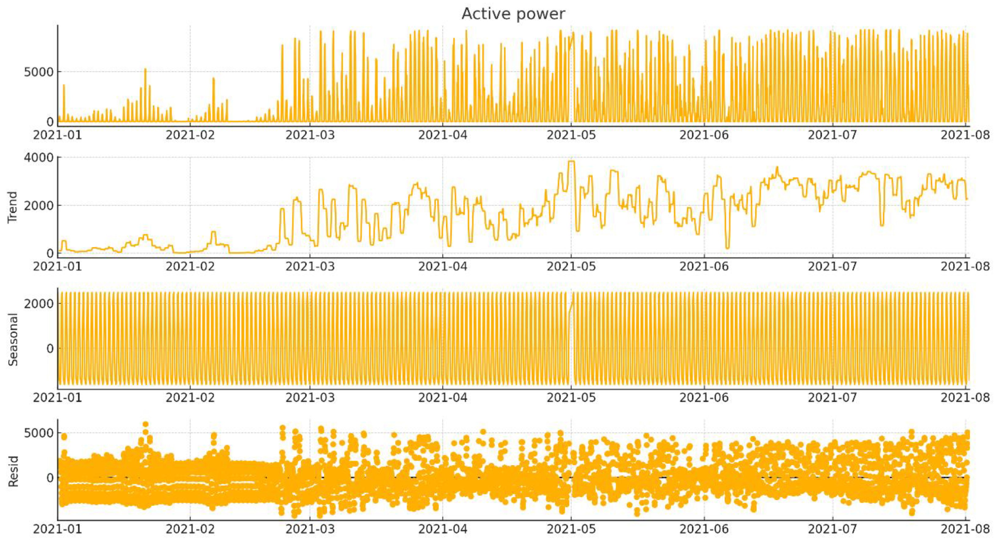
Figure 7.
Multiplicative decomposition of the active power time series.
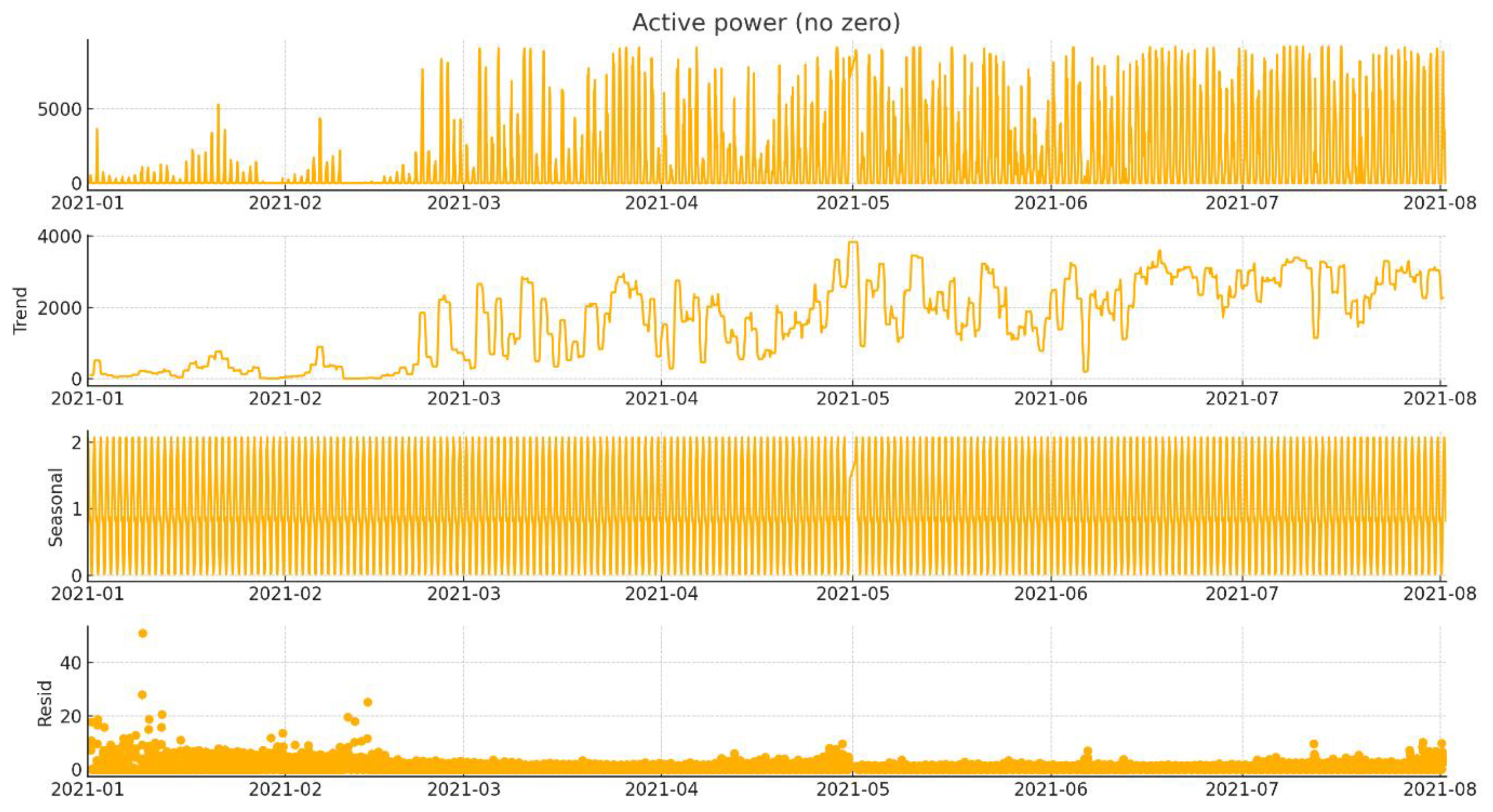
The additive Holt-Winters model assumes a constant seasonal amplitude, which does not align with the physical characteristics of PV generation. This assumption results in non-uniform residuals (Figure 6) and fails to reflect the observed fluctuations in solar energy output, especially across different seasons. In contrast, the multiplicative Holt-Winters model scales the seasonal component in proportion to the level of the time series, which more accurately captures the underlying dynamics of solar power generation. This model not only reflects seasonal variations more realistically but also adapts to gradual changes in energy output over time. Moreover, it produces residuals with more stable behaviour and lower dispersion (Figure 6), indicating a better fit to the data. Based on this analysis, the multiplicative Holt-Winters model was selected for forecasting, as it provides a more accurate and robust representation of the seasonal and trend behaviour of PV generation.
To complement the numerical evaluation, a visual inspection of the forecasted results was conducted. Figure 8 displays a representative three-day period (April 1-3, 2021), comparing actual PV power output with the predictions generated by each of the four models.
Figure 8.
Forecast comparison over a representative three-day period (April 1-3, 2021) using all evaluated models.
Figure 8.
Forecast comparison over a representative three-day period (April 1-3, 2021) using all evaluated models.
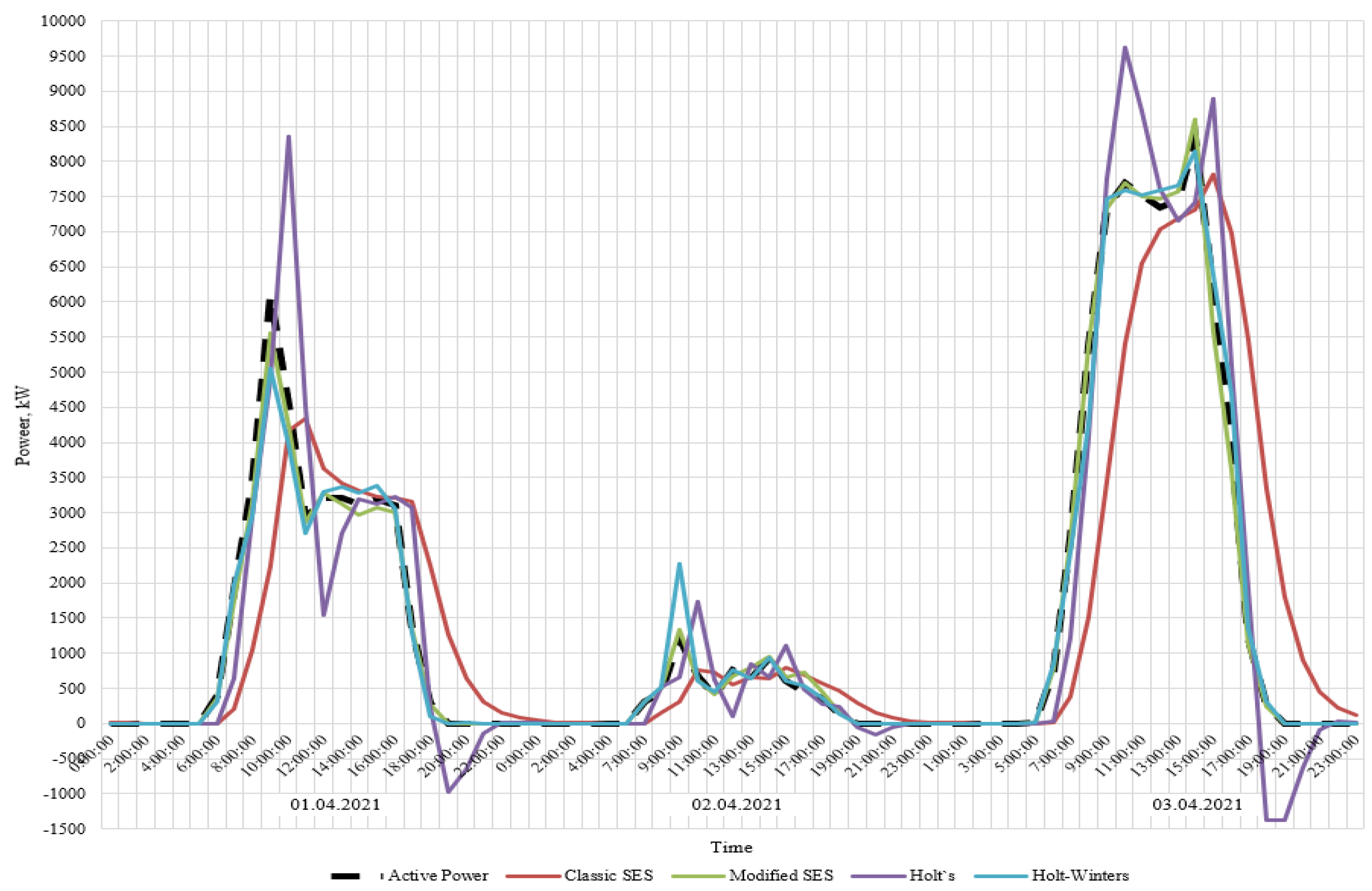
The three-day comparison in Figure 8 reveals distinct performance patterns among the evaluated models, especially in terms of their ability to replicate the diurnal structure of solar generation. Visual inspection of the forecast trajectories highlights how each model responds to sharp irradiance transitions, peak timing, and overnight stability.
On April 1, the Classic SES model exhibits a delayed response to the morning ramp-up and significantly overestimates evening values. Its forecast trajectory lacks the necessary reactivity to track the rapid power increases and decreases typical of clear-sky days. Conversely, the Modified SES and Holt-Winters models follow the actual power curve closely, accurately reflecting both the magnitude and shape of the generation peak. This suggests superior adaptability to daily solar patterns.
April 2 introduces a day with partially cloudy or variable conditions, as indicated by irregular midday dips in the actual power curve. The Holt’s model responds with excessive sensitivity, producing a fluctuating forecast with visible overshooting. The Classic SES again trails behind, lagging during the afternoon peak. In contrast, the Modified SES maintains a smoother trajectory, aligning well with the overall trend while dampening short-term noise. Holt-Winters also performs reliably but shows minor deviations during peak instability periods.
On April 3, the differences become even more pronounced during the midday plateau. While most models capture the steep morning rise with reasonable accuracy, the Classic SES continues to underestimate peak generation. Holt’s method overshoots during the noon hours, while the Modified SES and Holt-Winters remain consistently close to the actual values. Their ability to track both the amplitude and timing of generation transitions underlines their robustness.
In summary, this visual comparison confirms the conclusions drawn from the statistical evaluation. The Modified SES and Holt-Winters models exhibit the highest accuracy and adaptability across a range of irradiance conditions. The Classic SES, while computationally simple, fails to capture the dynamics of PV output, particularly under rapidly changing conditions. Holt’s method, although better suited for trend tracking, occasionally produces unstable predictions when faced with nonlinear variability.
Table 1 presents the comparative results across various accuracy metrics, highlighting significant differences in the predictive performance among the models.

Table 1.
Forecasting performance metrics for all models.
| Model | RMSE, kW | nRMSE, % | MAE, kW | nMAE, % | R2 |
|---|---|---|---|---|---|
| Classic SES | 1413.58 | 15.35 | 848.8 | 9.22 | 0.41 |
| Modified SES | 166.45 | 1.81 | 77.46 | 0.84 | 0.99 |
| Holt`s | 1052.79 | 11.43 | 548.59 | 5.96 | 0.94 |
| Holt-Winters | 1031.00 | 11.2 | 340.99 | 3.7 | 0.96 |
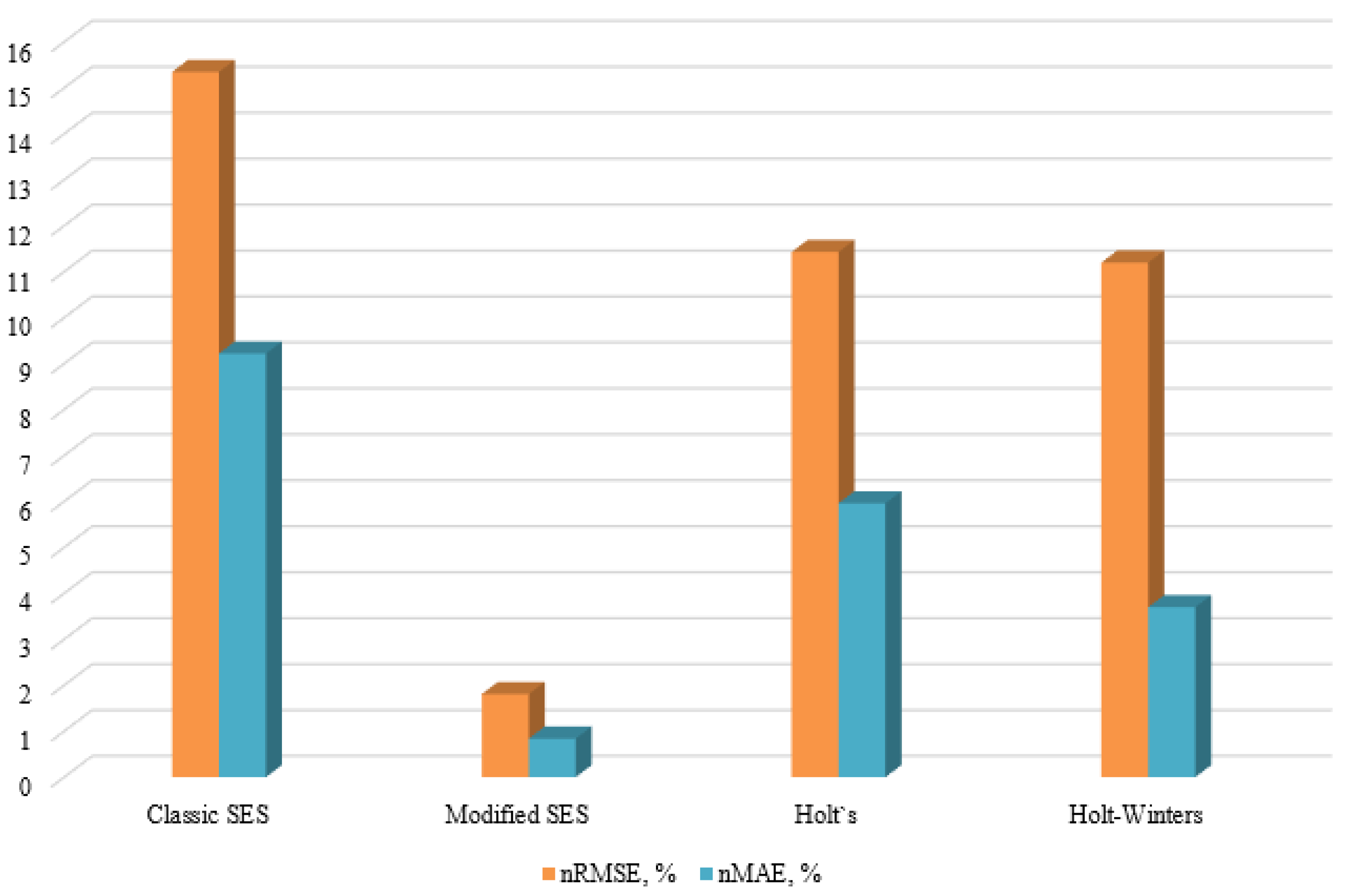
Additionally, for enhanced clarity, graphical comparisons of forecasting accuracy metrics are provided. Figure 9 presents a bar-line combination chart showing RMSE and MAE (in kW) alongside R² for each model. Figure 10 displays a grouped bar chart comparing nRMSE and nMAE (in %).
Figure 9.
Forecast comparison over a representative three-day period (April 1-3, 2021) using all evaluated models.
Figure 9.
Forecast comparison over a representative three-day period (April 1-3, 2021) using all evaluated models.
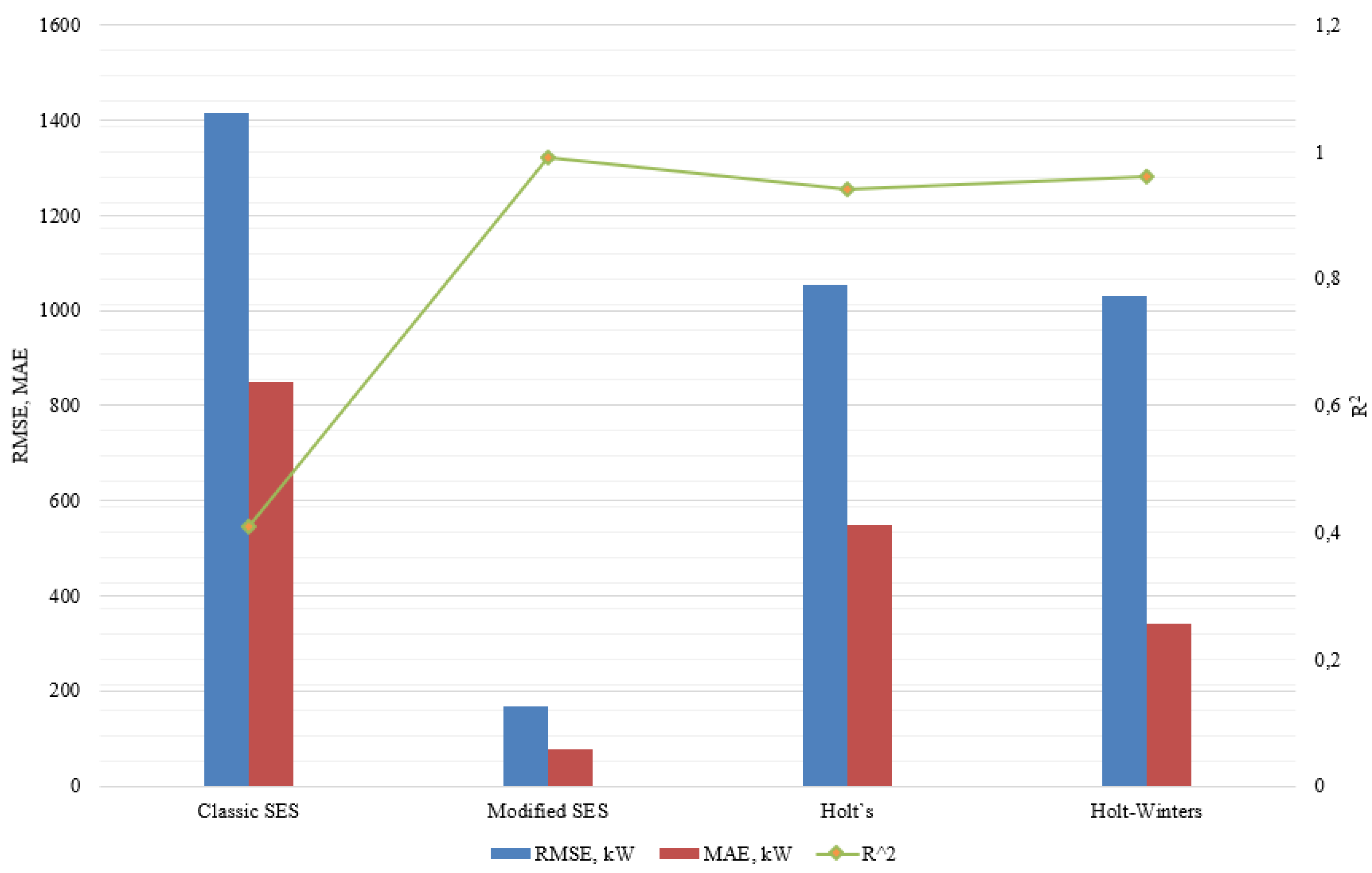
Figure 10.
Comparison of nRMSE and nMAE across all forecasting models.
The сlassic SES method demonstrated the least accurate forecasting performance, evident from its highest RMSE (1413.58 kW) and lowest R² (0.41). Such results indicate that сlassic SES struggled significantly in capturing the dynamics of the PV generation series, primarily because of its inherent assumption of a stationary time series without seasonal or trend variations. Given the clear seasonal and diurnal cycles observed in the PV data, it is unsurprising that this model produced substantial forecasting errors.
While SES remains popular for its simplicity and fast implementation, its practical limitations are increasingly recognised in the context of renewable energy forecasting. Several studies have attempted to evaluate its suitability for solar forecasting. For instance, [41] applied the SES method for forecasting PV generation from a 5 MW solar power plant in India. Their findings indicated that although SES was easy to implement, its performance degraded significantly in the presence of seasonal or trend-related patterns.
In contrast, Holt’s method offered a noticeable improvement in accuracy, with RMSE and MAE reduced to 1052.79 kW and 548.59 kW, respectively, and R² improving significantly to 0.94. This improvement can be attributed to Holt’s incorporation of a trend component, enabling the model to adapt better to gradual fluctuations over time. However, despite these improvements, Holt’s method did not account explicitly for seasonal patterns, limiting its accuracy, especially during periods of pronounced daily or seasonal variability.
Studies such as [42] demonstrated that Holt’s method can yield satisfactory results for short-term forecasting of PV generation, particularly when the primary concern is modelling linear trends over brief intervals. Their implementation in a practical context of solar forecasting highlights the method’s ease of use and relatively stable performance under mild seasonal variation. Similarly, in [43] it was explored a broader class of exponential smoothing, including triple exponential smoothing, but acknowledged the relevance of simpler models like Holt’s under constrained computational setups or minimal seasonal dynamics. When comparing these insights with our results, it becomes evident that while Holt’s model performs adequately in trend-dominant scenarios, it is less suitable when pronounced daily and seasonal cycles dominate, as is the case with our PV dataset.
The Holt-Winters model, particularly chosen in its multiplicative form due to the clear multiplicative seasonality observed in initial data analysis, achieved notable forecasting accuracy. With an RMSE of 1031.00 kW, an MAE of 340.99 kW, and a robust R² value of 0.96, Holt-Winters excelled in capturing both trend and seasonal fluctuations inherent in PV generation data. The multiplicative variant was specifically selected after preliminary model comparisons indicated that the PV output exhibited proportional seasonal variations that aligned closely with multiplicative model assumptions. The resulting model thus effectively mirrored the seasonal peaks and troughs, as demonstrated by its relatively low nMAE (3.7%) and nRMSE (11.2%).
While the multiplicative Holt-Winters model was selected in this study due to its ability to accurately capture the proportional seasonal variations inherent in PV power generation, alternative approaches in the literature have favoured the additive form. For instance, some studies have revisited the additive Holt-Winters method, proposing enhancements to its initial value calculations to improve forecasting accuracy in certain contexts [44]. These studies suggest that the additive model, which assumes constant seasonal fluctuations, can be effective in scenarios where the seasonal effect does not vary significantly with the level of the time series. However, in the context of PV power generation, where seasonal effects are multiplicative – i.e., the amplitude of seasonal variations increases with the level of solar irradiance – the multiplicative model provides a more realistic representation. This is particularly evident during summer months when higher irradiance levels lead to proportionally larger power outputs. Therefore, despite the existence of literature supporting the additive model in specific applications, the multiplicative Holt-Winters model is more appropriate for modelling PV power generation due to its capacity to accommodate the proportional nature of seasonal variations observed in the data. This is further supported in study [43], which demonstrated the capability of triple exponential smoothing to respond effectively to solar irradiance variability, underscoring the benefits of dynamic seasonal adjustment.
Most remarkably, however, the Modified SES model, explicitly tailored in this study by incorporating previous-day, same-hour values into its forecasting structure, significantly outperformed all other models. With the lowest recorded RMSE (166.45 kW) and MAE (77.46 kW), along with exceptionally high R² (0.99), this modification demonstrated superior predictive accuracy and consistency. The substantial improvement in forecasting precision can be explained by its direct alignment with the repetitive daily cycle inherent in PV generation. This modification not only leveraged recent historical data but also effectively integrated the critical diurnal pattern, dramatically enhancing forecast reliability.
The efficiency and interpretability of the Modified SES model are also noteworthy. Compared to the more computationally intensive Holt-Winters model, the Modified SES maintained a simple computational framework, crucial for real-time operational contexts such as Grid management or local energy storage optimisation. This model offered the best trade-off between computational simplicity and forecasting precision, thus emerging as a highly practical solution for hourly PV generation forecasting.
Figure 9 and Figure 10 support this evaluation. Figure 9 shows RMSE and MAE values for all models, overlaid with their respective R² scores. The Modified SES model distinctly leads across all three dimensions. Figure 10 complements this by comparing normalised errors, clearly indicating the Modified SES model’s dominant accuracy even after scale adjustment.
While SES remains popular for its simplicity and fast implementation, a review of the recent literature (2020-2024) revealed a lack of modern studies that focus on adapting or modifying SES specifically for PV power forecasting without hybridisation. Most works either apply SES in its classical form or integrate it into hybrid frameworks. To the best of our knowledge, there are no studies since 2020 that have proposed a comparable modification of SES as implemented in this research, namely, the integration of same-hour previous-day values into the smoothing process.
Summarising the comparative analysis, it is clear that simple, stationary-assumption-based models (like Classic SES) are significantly limited when forecasting data exhibiting pronounced daily or seasonal variations. Methods incorporating trend (Holt’s) or seasonality (Holt-Winters) markedly improve predictive accuracy but at an increased computational cost. However, the proposed Modified SES stands out as uniquely effective, offering near-perfect accuracy, minimal computational burden, and a high degree of interpretability. This combination of strengths strongly supports its adoption for practical forecasting applications in solar energy management.
In conclusion, while traditional exponential smoothing methods provide baseline forecasting capabilities, the integration of domain-specific modifications significantly enhances their predictive performance. The findings underscore the necessity of adapting classical forecasting approaches to specific operational characteristics – in this case, the daily and seasonal patterns inherent to PV generation.
6. Conclusions
This study conducted a comprehensive comparative evaluation of four exponential smoothing methods – Classic Simple Exponential Smoothing, Modified Simple Exponential Smoothing, Holt’s linear, and the Holt-Winters seasonal – for short-term forecasting of PV power generation based on real hourly operational data from a ground-mounted PV power plant in Ukraine. Unlike many studies that focus on solar irradiance, this research directly targeted the active power output of the PV system, aligning the forecasting objective with the practical needs of energy system management.
The Classic Simple Exponential Smoothing, though simple and computationally efficient, was inadequate for PV generation forecasting. Its inability to adapt to recurrent daily patterns led to the poorest performance across all metrics (R² = 0.41, high RMSE and nMAE values), underscoring its limitations for non-stationary, seasonally affected data.
Incorporating a trend component, Holt’s linear method improved forecasting performance (R² = 0.94) but still struggled during periods of rapid generation changes typical in PV output. Its lack of a seasonal component made it prone to inaccuracies, particularly during the steep morning and evening transitions.
The Holt-Winters method, applied in its multiplicative form following analysis of the seasonal characteristics of the data, demonstrated strong forecasting accuracy (R² = 0.96, nMAE = 3.7%). It effectively captured both trend and daily cyclical behaviour, making it well-suited for PV generation characterised by proportional seasonal fluctuations.
The most significant advancement was achieved with the Modified Simple Exponential Smoothing proposed in this study. By integrating previous-day, same-hour information into the forecasting framework, the Modified Simple Exponential Smoothing captured diurnal regularities while maintaining a simple, transparent structure. It achieved the highest accuracy (R² = 0.99, lowest RMSE and nMAE = 0.84%), outperforming both classical and more complex smoothing approaches. Its combination of low computational cost, easy implementation, and excellent predictive capability makes it a promising tool for real-time PV forecasting in Grid-connected and decentralised energy systems.
Overall, the results highlight the importance of tailoring forecasting models to the specific temporal structure of PV generation. Classic Simple Exponential Smoothing, while effective in some contexts, requires modifications to accurately reflect the pronounced daily cycles of solar output. The success of the Modified Simple Exponential Smoothing suggests that even simple models can achieve state-of-the-art performance when adapted to domain-specific patterns.
Future work could explore expanding the Modified Simple Exponential Smoothing approach to multi-step forecasting horizons, combining it with probabilistic modelling to address forecast uncertainty, or integrating exogenous weather information to enhance robustness under highly variable conditions.
Author Contributions
Conceptualization, D.M. and A.Z.; methodology, D.M., V.B. and M.K.; software, D.M.; validation, A.Z., M.K. and V.D.; formal analysis, D.M and V.D.; investigation, D.M. and A.Z.; resources, D.M. and A.Z.; data curation, D.M.; writing—original draft preparation, D.M. and A.Z.; writing—review and editing, A.Z., V.B. and M.K.; visualization, D.M.; supervision, V.B. and M.K.; project administration, D.M. and A.Z..; funding acquisition, A.Z. and V.D. All authors have read and agreed to the published version of the manuscript.
Funding
This research received no external funding.
Data Availability Statement
All data used in this study were obtained from operational measurements at a 9 MW grid-connected photovoltaic power plant located in Velyka Dymerka, Kyiv region, Ukraine. The dataset includes active power output recorded at 10-minute intervals over a seven-month period (January-July 2021). Due to confidentiality agreements with the plant operator, the raw dataset is not publicly available, but processed hourly-averaged data and methodological details are available from the corresponding author upon reasonable request.
Acknowledgments
This work was supported by projects “Integrated modeling for robust management of food-energy-water-social-environmental (FEWSE) nexus security and sustainable development” (IIASA-NASU, 22-501 (R-45-T)), “Comprehensive analysis of robust preventive and adaptive measures of food, energy, water and social management in the context of systemic risks and consequences of COVID-19” (0122U000552, 2022–2026), “Development of the structure and ensuring the functioning of self-sufficient distributed generation” (0125U001572, 2025-2026), which are financed by National Academy of Science of Ukraine.
Conflicts of Interest
The authors declare no conflicts of interest.
Abbreviations
The following abbreviations are used in this manuscript:
| CNN | Convolutional Neural Network |
| LSTM | Long Short-Term Memory |
| MAE | Mean Absolute Error |
| nMAE | Normalised Mean Absolute Error |
| PV | Photovoltaic |
| RMSE | Root Mean Square Error |
| SES | Simple Exponential Smoothing |
References
- Maliarenko, O.; Maistrenko, N.; Eutukhova, T. Factors Influencing the Forecast of Energy Consumption of the Country in the Conditions of War and the Amount of Reduction of Greenhouse Gas Emissions. Syst. Res. Energy 2024, 4, 65–76. [Google Scholar] [CrossRef]
- Kostenko, G.; Zaporozhets, A. Enhancing of the Power System Resilience through the Application of Micro Power Systems (Microgrid) with Renewable Distributed Generation. Syst. Res. Energy 2023, 3, 25–38. [Google Scholar] [CrossRef]
- Kostenko, G.; Zaporozhets, A.; Zaporozhets, N.; Verpeta, V. Aspects of Integrating Renewable Distributed Generation into the Energy Supply System of Ukraine. Probl. Econ. 2024, 2, 83–93. [Google Scholar] [CrossRef]
- Chaib, H.; Hassaine, S.; Mihoub, Y.; Moreau, S. Intelligent Power Control Strategy Based on Self-Tuning Fuzzy MPPT for Grid-Connected Hybrid System. Elect. Eng. Electromech. 2025, 3, 23–30. [Google Scholar] [CrossRef]
- Nechaieva, T.; Teslenko, O.; Trokhaniak, V.; Makarevych, S. Modelling the Energy Balances Community under Conditions Increasing Energy Independence and Reducing Greenhouse Gas Emissions. Machinery Energet. 2025, 16, 104–116. [Google Scholar] [CrossRef]
- Bosak, A.; Matushkin, D.; Dubovyk, V.; Homon, S.; Kulakovskyi, L. Determination of the Concepts of Building a Solar Power Forecasting Model. Sci. Horiz. 2021, 24, 9–16. [Google Scholar] [CrossRef]
- Chodakowska, E.; Nazarko, J.; Nazarko, Ł.; Rabayah, H.S. Solar Radiation Forecasting: A Systematic Meta-Review of Current Methods and Emerging Trends. Energies 2024, 17, 3156. [Google Scholar] [CrossRef]
- Suanpang, P.; Jamjuntr, P. Machine Learning Models for Solar Power Generation Forecasting in Microgrid Application: Implications for Smart Cities. Sustainability 2024, 16, 6087. [Google Scholar] [CrossRef]
- Waqas, M.; Humphries, U.W.; Chueasa, B.; Wangwongchai, A. Artificial Intelligence and Numerical Weather Prediction Models: A Technical Survey. Nat. Hazards Res. 2024, 5, 306–320. [Google Scholar] [CrossRef]
- Girdhani, B.; Agrawal, M. Performance Evaluation of Statistical and Deep Learning Models for Daily Solar Global Horizontal Radiation Prediction: Implications for Renewable Energy and Sustainability. Environ. Dev. Sustain. 2025. [Google Scholar] [CrossRef]
- Matushkin, D.; Bosak, A. Design of a MATLAB GUI for Short-Term Solar Forecasting Based on Deep Learning. Vidnovl. Energet. 2023, 3, 32–41. [Google Scholar] [CrossRef]
- Bosak, A.; Matushkin, D.; Davydenko, L.; Kulakovskyi, L.; Bronytskyi, V. Short-Term Forecasting of Photovoltaic Solar Power Generation Based on Time Series: Application for Ensure the Efficient Operation of the Integrated Energy System of Ukraine. In Power Systems Research and Operation; Kyrylenko, O., Denysiuk, S., Derevianko, D., Blinov, I., Zaitsev, I., Zaporozhets, A., Eds.; Springer: Cham, Switzerland, 2023; Volume 220, pp. 159–179. [Google Scholar] [CrossRef]
- SolarPower Europe. Global Market Outlook for Solar Power 2025–2029. 2025. Available online: https://www.solarpowereurope.org/insights/outlooks/global-market-outlook-for-solar-power-2025-2029.
- StartUs Insights. Photovoltaic Market Outlook 2025. 2025. Available online: https://www.startus-insights.com/innovators-guide/photovoltaic-market-outlook/.
- Leyva, M. Solar: Predictions for 2025. Wood Mackenzie 2025. Available online: https://www.woodmac.com/news/opinion/solar-2025-outlook/.
- Lindström, S. Expert Analysis: The Three Strongest Solar Energy Trends in 2025. PV Europe 2025. Available online: https://www.pveurope.eu/markets/expert-analysis-three-strongest-solar-energy-trends-2025.
- ISO New England. Final 2025 Photovoltaic (PV) Forecast. 2025. Available online: https://www.iso-ne.com/static-assets/documents/100022/2025_final_pv_forecast.pdf.
- Thompson, A. Employing Sky Images for Ultra-Short-Term Solar Forecasts. Scilight 2025, 131106. [Google Scholar] [CrossRef]
- Wang, L.; Li, X.; Hao, Y.; Zhang, Q. Ultra-Short-Term Solar Irradiance Prediction Using an Integrated Framework with Novel Textural Convolution Kernel for Feature Extraction of Clouds. Sustainability 2025, 17, 2606. [Google Scholar] [CrossRef]
- Sun, X.; Zhang, W.; Ren, M.; Zhu, Z.; Yan, G. Ultrashort-Term Prediction of Solar Irradiance with Multiple Exogenous Variables by Fusion of Ground-Based Sky Images. Journal of Renewable and Sustainable Energy 2025, 17, 023501. [Google Scholar] [CrossRef]
- Khasyshyn, N.; Liubinskyi, B. Forecasting Solar Energy Generation Using Deep Learning Models. Mathematical Modeling and Computing 2025, 12, 669–681. [Google Scholar] [CrossRef]
- El Aouni, A.; Naimi, S.E.; Ayat, Y. Machine Learning-Based Photovoltaic Power and Energy Prediction in Time–Frequency Domain. Electrical Engineering 2025. [Google Scholar] [CrossRef]
- Attya, M.; Abo-Seida, O.; Mohamed, H.; Mohammed, A. A Hybrid Deep Learning Framework for Solar Irradiation Prediction Based on Regional Satellite Images and Data. Neural Computing and Applications 2025, 37, 14327–14363. [Google Scholar] [CrossRef]
- Bo, L.; Elnaggar, A.; Elattar, M.; El-Raey, M. Forecasting of Solar Irradiance and Power in Uncertain Photovoltaic Systems Using Bi-LSTM and Bayesian Optimization. Arabian Journal for Science and Engineering 2024, 49, 1347–1365. [Google Scholar] [CrossRef]
- Mishra, A.; Ravindra, T.; Iyengar, S.; Kalyanaraman, S.; Kumaraguru, P. SPIRIT: Short-Term Prediction of Solar Irradiance for Zero-Shot Transfer Learning Using Foundation Models. arXiv 2025, arXiv:2502.10307. [Google Scholar] [CrossRef]
- Teja, U.V.; Kiran, M.S.; Karthikeya, V.; Murali, E.; Kumanan, T. Solar Radiation Prediction Using Machine Learning and Python. International Journal of Science and Advanced Technology 2025, 16, 2713–2721. [Google Scholar] [CrossRef]
- Svetunkov, I.; Kourentzes, N.; Ord, J.K. Complex Exponential Smoothing. Naval Research Logistics 2022, 69, 1108–1123. [Google Scholar] [CrossRef]
- Iheanetu, K.J. Solar Photovoltaic Power Forecasting: A Review. Sustainability 2022, 14, 17005. [Google Scholar] [CrossRef]
- Akhtar, S.; Shahzad, S.; Zaheer, A.; Ullah, H.S.; Kilic, H.; Gono, R.; Jasiński, M.; Leonowicz, Z. Short-Term Load Forecasting Models: A Review of Challenges, Progress, and the Road Ahead. Energies 2023, 16, 4060. [Google Scholar] [CrossRef]
- Waheed, W.; Qingshan, X. An Efficient Load Forecasting Technique by Using Holt-Winters and Prophet Algorithms to Mitigate the Impact on Power Consumption in COVID-19. IET Energy Syst. Integr. 2024, 6, 364–374. [Google Scholar] [CrossRef]
- Boland, J. Constructing Interval Forecasts for Solar and Wind Energy Using Quantile Regression, ARCH and Exponential Smoothing Methods. Energies 2024, 17, 3240. [Google Scholar] [CrossRef]
- Svetunkov, I.; Kourentzes, N.; Ord, J.K. Complex Exponential Smoothing. Naval Res. Logist. 2022, 69, 1108–1123. [Google Scholar] [CrossRef]
- Rosita, Y.D.; Moonlight, L.S. Perbandingan Metode Prediksi untuk Nilai Jual USD: Holt-Winters, Holt’s, dan Single Exponential Smoothing. J. Teknol. Inform. Multimedia 2024, 5, 322–333. [Google Scholar] [CrossRef]
- Ostertagova, E.; Ostertag, O. Forecasting Using Simple Exponential Smoothing Method. Acta Electrotech. Inform. 2012, 12, 62–66. [Google Scholar] [CrossRef]
- Omer, A.; Blbas, H.; Kadir, D. A Comparison between Brown’s and Holt’s Double Exponential Smoothing for Forecasting Applied Generation Electrical Energies in Kurdistan Region. Cihan Univ. Erbil Sci. J. 2021, 5, 56–63. [Google Scholar] [CrossRef]
- Zaichenko, S.; Trachuk, A.; Shevchuk, N.; Pochka, K.; Shalenko, V. Forecasting the Development of Renewable National Energy in the Tourism Sector of Ukraine. E3S Web Conf. 2024, 508, 02006. [Google Scholar] [CrossRef]
- Alay, F.D.; İlhan, N.; Güllüoğlu, M.T. A Comparative Study of Data Mining Methods for Solar Radiation and Temperature Forecasting Models. J. Univ. Comput. Sci. 2024, 30, 847–877. [Google Scholar] [CrossRef]
- İnce, M.N.; Taşdemir, Ç. Forecasting Retail Sales for Furniture and Furnishing Items through the Employment of Multiple Linear Regression and Holt–Winters Models. Systems 2024, 12, 219. [Google Scholar] [CrossRef]
- Abdelati, M.H.; Abdelwali, H.A. Optimizing Simple Exponential Smoothing for Time Series Forecasting in Supply Chain Management. Indones. J. Innov. Appl. Sci. 2024, 4, 247–256. [Google Scholar] [CrossRef]
- Lim, P.; Nayar, C. Solar Irradiance and Load Demand Forecasting Based on Single Exponential Smoothing Method. Int. J. Eng. Technol. 2012, 4, 451–455. [Google Scholar] [CrossRef]
- Pratap Singh, V.; Srivastava, P. Single Exponential Smoothing Approach for 5 MW Solar Power Plant Generation Forecasting. Power Res.—A J. CPRI 2015, 573–576. https://cprijournal.in/index.php/pr/article/view/713.
- Kim, E.G.; Akhtar, M.S.; Yang, O.B.; Lee, B.T. Designing Solar Power Generation Output Forecasting Methods Using Time Series Algorithms. Elect. Power Energy Syst. 2023, 216, 109073. [Google Scholar] [CrossRef]
- Dev, S.; AlSkaif, T.; Hossari, M.; Godina, R.; Louwen, A.; van Sark, W. Solar Irradiance Forecasting Using Triple Exponential Smoothing. arXiv 2018. [Google Scholar] [CrossRef]
- Hansun, S.; Charles, V.; Indrati, C.R.; Subanar. Revisiting the Holt-Winters’ Additive Method for Better Forecasting. Int. J. Enterp. Inf. Syst. 2019, 15, 43–57. [Google Scholar] [CrossRef]
Disclaimer/Publisher’s Note: The statements, opinions and data contained in all publications are solely those of the individual author(s) and contributor(s) and not of MDPI and/or the editor(s). MDPI and/or the editor(s) disclaim responsibility for any injury to people or property resulting from any ideas, methods, instructions or products referred to in the content. |
© 2025 by the authors. Licensee MDPI, Basel, Switzerland. This article is an open access article distributed under the terms and conditions of the Creative Commons Attribution (CC BY) license (https://creativecommons.org/licenses/by/4.0/).
Copyright: This open access article is published under a Creative Commons CC BY 4.0 license, which permit the free download, distribution, and reuse, provided that the author and preprint are cited in any reuse.


