
Submitted:
10 June 2025
Posted:
10 June 2025
You are already at the latest version
Abstract
The increasing penetration of photovoltaic solar energy has intensified the need for accurate production forecasting to ensure efficient grid operation. This study critically compares traditional statistical methods and machine learning approaches for forecasting solar irradiance using the benchmark Folsom PLC dataset. Two primary research questions are addressed: whether machine learning models outperform traditional techniques, and whether time series modelling improves prediction accuracy. The analysis evaluates a range of models—statistical regressions (OLS, LASSO, Ridge), regression trees, neural networks, and random forests—applied to physical modelling and time series approaches. Results reveal that while machine learning methods can outperform statistical models, particularly with the inclusion of exogenous weather features, they do not universally dominate across all forecasting horizons. Furthermore, pure time series approach models show lower performance. However, a hybrid approach integrating physical models with machine learning, demonstrates significantly improved accuracy. These findings highlight the value of hybrid models for photovoltaic forecasting and suggest strategic directions for operational implementation.
Keywords:
time series
; forecasting
; PV
; management
; solar
; energy
; machine learning
1. Introduction
Production management in modern electrical systems is one of the fundamental pillars for ensuring the stability, efficiency, and sustainability of energy supply. System reliability and cost minimisation are the primary goals. One of the main operational challenges is maintaining a dynamic balance between electricity demand and available generation in real time. Since electricity is not easily storable, a precise production-service balance is essential to avoid both energy waste and risks of blackouts or grid overloads [1].
The increasing integration of renewable energy sources, especially intermittent ones like photovoltaic solar and wind, has profoundly transformed the structure and dynamics of electrical systems. While traditional sources such as thermal, nuclear, and even hydroelectric plants allowed for highly controlled production management, new renewable plants depend heavily on weather conditions and are generally more volatile [2].
However, current regulations in many countries give dispatch priority to renewables, forcing their use over more controllable sources. While environmentally beneficial, this introduces significant complexity in system operation [3].
Photovoltaic solar energy, in particular, has seen exponential growth in recent years. As of 2024, global installed solar capacity exceeded 1,400 GW, with annual production reaching 2,000 TWh—about 7% of global electricity generation [4]. This growth is driven by technological cost reductions, incentive policies, and increasing environmental awareness.
Forecasting production has become central to management. Planning and scheduling of production units are based on demand forecasting, and effective management of this new energy reality also requires forecasting renewable energy production. While traditional models relied on statistical techniques, Machine Learning (ML) approaches have gained significant relevance in recent years. These algorithms have shown superior ability to capture nonlinear patterns and adapt to highly variable contexts.
This article critically reviews the primary forecasting methods applied to electricity production management, with a special focus on ML models. Their performance is evaluated using a widely used dataset in scientific literature: the Folsom photovoltaic plant data [5]. This facility has become a benchmark for validating predictive models due to its data availability and quality. Two research questions are addressed in the article:
- RQ1: Are ML methods more accurate than traditional methods?
- RQ2: Can the use of time series enhance forecast accuracy?
2. Related Literature
Reliability in photovoltaic (PV) production forecasting is essential for properly functioning the power system. Forecasting errors in Europe range between 15% and 100%, measured as normalised RMSE relative to the mean [6]. A significant portion of this error is influenced by weather conditions, which can introduce up to 35% RMSE in predictions [7].
This forecasting error propagates from generation to the grid, operated by a Transmission System Operator (TSO) or an Independent System Operator (ISO), ultimately impacting distribution networks. Although the economic cost of this error is difficult to generalise, it is estimated to range between 40 and 140 USD/MWh [8]. With the substantial increase in PV generation currently underway, this impact is likely to grow. Consequently, there is a growing interest in improving forecasting accuracy [9].
The fundamental element in forecasting is solar irradiance. Generally, two distinct methodological approaches are employed: those based on time series data and those relying on physical models [10].
Forecasting based on physical models initially estimates irradiance under favourable weather conditions, known as clear-sky conditions. These models use cell temperature to calculate power output. Notable examples include the Nominal Operating Cell Temperature (NOCT) models [11] and the Sandia models [12], developed by Sandia National Laboratories. Comparative studies indicate minimal differences in performance between these models [13]. These models are subsequently adjusted using meteorological data, so that the final irradiance estimate accounts for cloud cover, wind, and other atmospheric conditions [14].
In this context, the integration of satellite imagery with radiative transfer physical models to estimate surface solar irradiance at high spatial and temporal resolution has shown improved results [15]. SoDa (Solar radiation Data) is a platform providing access to solar irradiance databases and estimation models, such as HelioClim and the Heliosat-2 model, developed by MINES ParisTech [16]. Bu, Qiangsheng et al. [17] combine spatiotemporal analysis of satellite images interpreted through convolutional neural networks (CNNs) and LSTM (Long Short-Term Memory) networks to simulate the impact of cloud cover on irradiance.
Forecasting using statistical and time series models is applied to direct irradiance estimation and to predicting meteorological parameters that influence irradiance, thereby complementing physical models [18]. Classical time series methods are common—Singh & Garg [19] and Sapundzhi et al. [20] employ ARIMA-based models, although hybrid models incorporating ML are generally preferred. Despotovic et al. [21] use autoregressive models with transfer learning to forecast PV output in Spain. Torres et al. [22] developed a deep learning-based solar power forecasting system that integrates multiple data sources (meteorological, historical production, satellite, etc.). The model combines CNNs to extract spatial features from meteorological data and LSTM networks to capture temporal dynamics. This integration significantly enhances predictive performance compared to traditional models, even when applied to large datasets [23]. Xu et al. [24] present a hybrid short-term PV output forecasting approach that combines signal decomposition with the XGBoost model (Extreme Gradient Boosting).
In order to promote research in this field, several noteworthy initiatives have been undertaken to share solar production data openly [25]. As the integration of PV systems into electric grids increases, it becomes essential to improve forecasting methods.
A clear example is the dataset released by Pedro et al. [5], commonly referred to as the PLC dataset. This dataset is widely used for benchmarking forecasting models.
Marinho et al. [26] explore short-term solar irradiance forecasting using deep learning techniques (CNN-1D, LSTM, and CNN-LSTM) applied to the Folsom (USA) dataset.
Oliveira et al. [27] develop a novel architecture and use the Folsom data for benchmarking. Yang et al. [28] compare models such as Quantile Regression Forests, Gaussian Process Regression, Bayesian Model Averaging, Ensemble Model Output Statistics (EMOS), and Persistence-based probabilistic models, also using the same dataset. Oliveira et al. [29] apply a Quantum Neural Network (QNN) for forecasting, again leveraging the Folsom dataset.
3. Materials and Methods
3.1. Dataset
This study uses a freely available Dataset obtained from the Zenodo repository under the DOI: 10.5281/zenodo.2826939, commonly called the Folsom PLC Dataset. This Dataset was provided by Pedro et al. [5] and contains detailed measurements from the California Independent System Operator (CAISO) headquarters located in Folsom, CA, USA. The data includes single-minute frequency recordings of global horizontal irradiance (GHI) and direct normal irradiance (DNI), as well as some weather conditions: ambient temperature, relative humidity, wind speed and direction, pressure, etc.
In addition to on-site measurements, the dataset also includes meteorological forecast variables obtained from the North American Mesoscale Forecast System (NAM), sky images and satellite images.
The primary reason for selecting this dataset is its extensive use in the scientific community. The Folsom PV Dataset has been widely studied in the context of photovoltaic power forecasting, and it serves as a benchmark in numerous research articles. Its frequent use in the literature enables consistent comparisons across different predictive modelling approaches, thereby facilitating objective evaluation of model performance. Moreover, its public availability and data quality make it particularly suitable for reproducible and comparative research.
Several studies have utilised this dataset to assess and benchmark solar forecasting approaches. For example, it has served as the basis for evaluating probabilistic forecasting methods using ensemble and hybrid models ([28,30]), as well as for implementing deep learning and quantum neural networks in solar irradiance prediction [31].
3.2. Machine Learning Methods
This study considered all machine learning methods capable of providing regression-based predictions. However, only those that yielded the best results are presented here. We show a brief description of each model.
3.2.1. Neural Networks
Neural network models are based on computational models formed by interconnected functional nodes called neurons [32]. Figure 1 shows a neuron of the network in detail. Each neuron produces an output signal () processing input signals using () through an activation function ().
Each neuron () is connected via links () called axons, which weigh the input the neuron receives. Additionally, biases () are added to increase model flexibility. Each neuron is connected to several input signals () that could be outputs from other neurons, or the predictor variables.
The activation function introduces non-linearity and can be linear, sigmoid, tanh, ReLU, etc., depending on the network’s purpose. The output of a neuron is calculated as in (1).
Neurons are organised into layers as shown in Figure 2. The layers are named input, hidden, and output. A common type is the feedforward neural network, consisting of one input layer, one or more hidden layers, and one output layer. It can be seen how the input variables (predictors, ) are linked to neurons lying in the input layer, which all must have the same number of observations . This data can either be endogenous or exogenous. The neurons in the output layer provide steps ahead forecasts of the output variable . The general formulation is shown in (2):
Training involves adjusting weights to minimise the difference between predicted and actual values, typically using gradient descent and a loss function like Mean Squared Error (MSE).
3.2.2. Regression Trees
Regression trees (RT) are a specific application of decision trees (DT) [33], which predict values by recursively partitioning the data based on predictor variables, similarly as regression does. The way the information is graphed reminds one of a tree, where each node splits into branches until reaching a terminal node (leaf) containing the response value. Figure 3 shows a generic representation of the tree.
At each internal node , starting from the root node, a decision is made regarding the path to follow, based on the splitting criterion defined at that node, which determines the behavior of the branch from that point onward, called region (). This process is repeated until leaf nodes are reached, at the bottom of the tree. Given a dataset depending on the splitting criteria, a leaf node is reached, from which the value is obtained as node value. The value at each internal node () is computed as the weighted average of the values of the downstream branches (regions, also known as rectangles) from that node.
To construct the tree structure and determine the splitting criteria, algorithms rely on error computation through specific metrics, with the most common one for regression being CART (Classification and Regression Trees). The process of constructing a RT involves determining the optimal number of terminal nodes, , as well as selecting a regularisation parameter that balances the trade-off between model complexity and data fitting. A larger number of nodes typically allows the model to capture more intricate patterns in the data, but it also increases the risk of overfitting. Conversely, a smaller tree may generalise better but at the cost of reduced accuracy.
A cost-complexity pruning approach is commonly employed to address this trade-off, where the objective is to minimise the function (3).
Here, is the number of terminal nodes in the tree, and is a non-negative parameter that penalises tree complexity. Optimal values of T and α are typically obtained through cross-validation. This involves partitioning the dataset into training and validation subsets, fitting trees with varying complexity, and selecting the configuration that minimises the cross-validated error. This procedure ensures that the final model achieves a good balance between predictive accuracy and generalisation capability.
3.2.3. Random Forest Ensemble
The combination of simple processes yields remarkable results. This philosophy underpins the foundation of ensemble methods based on DT. These methods enhance prediction accuracy by combining simpler models. Among them, Random Forest (RF) stands out as a robust technique that has consistently delivered strong performance [34].
Initially, the Bagging (Bootstrap Aggregating) technique is applied. See Figure 4 for a better understanding. This method involves dividing the dataset into training subsets , on which a series of sampling operations with replacement are performed. Simple models—RT in this case—are then fitted to each subset. Each sample drawn is independent from the others, which contributes to increasing the variability among the models.
A Random Forest is an ensemble of regression trees, where each tree is trained on a different bootstrap sample of the original dataset, introducing a layer of randomness. Specifically, a random subset of features is selected at each split within a tree, from which the best split is chosen. The purpose of this technique lies in its ability to decorrelate the trees, which significantly enhances the generalisation capacity of the ensemble and reduces overfitting.
The final prediction of a regression model based on RF is generally obtained by averaging the outputs of all individual trees. This aggregation smooths out the variance inherent in single DTs, resulting in more stable and accurate predictions.
3.3. Analysis
Based on the research questions posed, a structured methodology was defined with the primary objective of analysing the behaviour of various ML models. Given that energy production is highly dependent on solar irradiance, the prediction process focused specifically on estimating two key components: DNI and GHI.
The study was organised into two main research branches. The first focused on physical modelling approaches related to cell temperature estimation. The second branch explored time series forecasting based on historical production data.
A hybrid methodology was implemented for the physical modelling approach. Initially, cell temperature was estimated using a clear-sky model. This model was subsequently refined by integrating meteorological parameters using statistical and machine learning methods.
In contrast, the time series approach relied solely on ML models. Historical datasets, including energy production and weather-related variables, were used to train the models and generate forecasts.
4. Results
4.1. Physical Methods with Climate Features
Following the methodology described in [5], forecasts of both global and direct irradiance have been performed using a clear-sky model and by generating predictions for the clear-sky index , defined as the ratio between the actual irradiance and the theoretical clear-sky irradiance as seen in (4).
On the one hand, predictions are made using only endogenous variables; on the other hand, the model is extended by including exogenous variables.
The procedure involves first computing the clear-sky irradiance values—global horizontal irradiance () and direct normal irradiance ()—using the Ineichen and Perez model [35], which accounts for site-specific parameters such as atmospheric pressure and air mass. Once the clear-sky values are estimated, the predictive model is used to forecast the corresponding clear-sky index:
The choice of the physical model was motivated by the need to establish a baseline for comparison with the work presented in [5]. Although other models, such as those referenced, were considered, the minimal differences in performance led to the decision to retain the original approach.
As a result, the estimation of becomes the central focus of this analysis. Three prediction horizons have been considered: intra-hour (5 to 30 minutes ahead), intra-day (30 to 180 minutes ahead), and day-ahead (26 to 36 hours ahead). Forecasts have been made for a single time step ahead for each horizon.
The models employed were ordinary least squares (OLS), Ridge regression, and least absolute shrinkage and selection operator (LASSO). Owing to space limitations, a detailed account of the methods is omitted. Readers are referred to [36] for thorough and accessible explanations. In this study, we have utilised the same statistical models and, additionally, tested several ML models: RT, RF, neural networks (NN), LSTM, Support Vector Machines (SVM), among others. Only those models that yielded the best results are reported in this work. The forecasting results are presented in Table 1 for GHI and Table 2 for DNI.
An analysis of both tables indicates that, although increasing the forecasting horizon does not lead to a dramatic rise in RMSE values, the variability of this metric does increase significantly. This pattern is observed for both GHI and DNI. It is also evident that including exogenous variables, such as meteorological data, does not consistently enhance the predictive performance. While such variables contribute to improved results for intra-hour and next-day horizons, they do not offer benefits for intraday forecasts.
However, the comparison between ML and statistical models does not clearly favour either approach. While RF methods tend to show improvements in most cases, the other ML techniques do not consistently outperform the metrics achieved by statistical models, despite optimising their hyperparameters.
It can be concluded that, in this case, the use of ML does not provide a competitive advantage in operational terms: the performance metrics are very similar, while the time investment required to develop the models is significantly greater.
4.2. Time Series Approach
The previous analysis employed a strategy in which regression models were trained to generate predictions for a single future time step. In this approach, the endogenous variables described in [5] —namely , , and —served as input features to inform future forecasts. calculates the backward average of ; stands for the lagged average values and represents the variability of . While this method proved functional, using time series, the present analysis aims to adopt an alternative strategy more closely aligned with time series modeling.
Specifically, the objective is to explore the potential benefits of utilising the full temporal spectrum of the series, capturing its dynamic behaviour over time rather than focusing solely on individual time steps. ML techniques have been selected as the modelling framework to enable this expanded approach, thereby continuing and building upon the exploratory work initiated in the prior analysis.
In this context, the entire time series is utilised, including periods during which no production occurs, or is not expected to occur, since irradiance data occasionally reflect non-zero values under such conditions. The prediction is performed directly on the GHI and DNI values, rather than on derived indices. To capture the seasonality inherent in the time series, and following an approach similar to that proposed in [37], synthetic variables are introduced. Among these, the most notable is the 24-hour lagged version of the target variable, which is incorporated regardless of the forecasting horizon, as it encapsulates daily cyclic behaviour.
To account for potential trends, the series includes a moving average variable computed from the data 24 hours prior. This feature is also incorporated independently of the prediction horizon.
Finally, a hybrid approach has been considered, in which the calculation of , as used in the initial analysis, is retained, but enhanced by incorporating the previously mentioned time series features. In this way, the series is treated as a time series, including its seasonality and trend components. The key difference lies in the influence of the physical model, which varies depending on the time of year, while the index typically exhibits highly stochastic behaviour. The forecasts are made thus using (4).
Table 3 compares performance metrics for the prediction of DNI using ML models with a time series approach. Similarly, Table 4 provides the corresponding comparison for GHI.
The analysis of the results indicates that applying a time series model approach with this strategy does not enhance prediction performance; on the contrary, it degrades it. When using the original data directly as a time series, the inherent variability within the series interferes with the model’s predictions, as the model is unable to respond to rapid fluctuations effectively.
However, when a hybrid strategy is applied, the results improve significantly. In this approach, a physical model accounts for the influence of the sun’s position on the panels and the corresponding irradiance. This allows the ML models to focus solely on capturing the meteorological patterns, leading to more accurate and stable predictions.
5. Discussion
To address RQ1: Are ML methods more accurate than traditional methods?, this study used the dataset provided in [5], one of the most widely used benchmarks in the field. A comparison was carried out between traditional statistical models and ML models. While it is acknowledged that both statistical and ML approaches could be further refined and optimised to achieve better performance by developing tailored and highly customised models, the comparative analysis based on standard configurations reveals a clear trend: ML models outperform traditional statistical methods under comparable conditions. This suggests that even without extensive fine-tuning, ML techniques provide a more robust framework for solar irradiance forecasting.
Concerning RQ2: Can the use of time series enhance forecast accuracy?, the study explored a time series modelling approach by incorporating seasonality and temporal patterns present in the data. The findings indicate that traditional physical models are inherently better suited to handle the structure of irradiance data, mainly due to their ability to capture the deterministic components related to solar geometry. However, when a hybrid strategy is adopted—combining a physical model with a ML component—the predictive performance improves significantly. This hybrid approach leverages the strengths of physical models to manage solar position and irradiance incidence, while allowing ML models to focus on capturing meteorological variability. Therefore, while the exclusive use of time series modelling with raw data may not improve accuracy and can even degrade it, using time series techniques within a hybrid framework confirms, with some nuance, that temporal strategies can enhance forecast performance.
6. Conclusions
This study has comprehensively analysed using a widely adopted benchmark dataset in the solar energy forecasting field. The experimental framework has allowed for a fair and insightful comparison between traditional statistical approaches and ML models, considering both direct implementation and time series-based strategies.
The research questions posed at the outset have been effectively addressed. The results demonstrate that ML models provide a superior alternative to traditional statistical methods for the task of solar photovoltaic irradiance forecasting. This is particularly evident when time series strategies are employed, especially in hybrid configurations integrating physical modelling with ML. Such strategies enable better handling of the data’s deterministic and stochastic components, leading to improved prediction accuracy.
Naturally, the conclusions drawn here are specific to the scope and dataset of this study. However, the methodology and insights are transferable to other contexts. Work is already underway to apply this approach to additional datasets, to develop more generalisable conclusions and validate the observed trends across varying geographic and climatic conditions.
Future work will focus on the real-time implementation of similar models to integrate these forecasting strategies into operational systems for solar energy management and optimisation.
Author Contributions
Conceptualisation, O.T., J.C.G-D and A.P-S; methodology, O.T. and J.C.G-D.; software, O.T.; validation, O.T., J.C.G-D and A.P-S.; writing—original draft preparation, O.T.; writing—review and editing, J.C.G-D and A.P-S. All authors have read and agreed to the published version of the manuscript.
Data Availability Statement
Data is available at https://zenodo.org/records/2826939.
Conflicts of Interest
The authors declare no conflicts of interest.
References
- Mathiesen, B.V.; Lund, H.; Connolly, D.; Wenzel, H.; Østergaard, P.A.; Möller, B.; Nielsen, S.; Ridjan, I.; Karnøe, P.; Sperling, K.; et al. Smart Energy Systems for coherent 100% renewable energy and transport solutions. Appl. Energy 2015, 145, 139–154. [Google Scholar] [CrossRef]
- Albadi, M.; El-Saadany, E. A summary of demand response in electricity markets. Electr. Power Syst. Res. 2008, 78, 1989–1996. [Google Scholar] [CrossRef]
- IEA Renewables 2023. 2028.
- REN21 Renewables 2024 Global Status Report Collection; Paris. 2024.
- Pedro, H.T.C.; Larson, D.P.; Coimbra, C.F.M. A comprehensive dataset for the accelerated development and benchmarking of solar forecasting methods. J. Renew. Sustain. Energy 2019, 11, 036102. [Google Scholar] [CrossRef]
- Zsiborács, H.; Pintér, G.; Vincze, A.; Baranyai, N.H.; Mayer, M.J. The reliability of photovoltaic power generation scheduling in seventeen European countries. Energy Convers. Manag. 2022, 260. [Google Scholar] [CrossRef]
- Brusco, G.; Burgio, A.; Menniti, D.; Pinnarelli, A.; Sorrentino, N.; Vizza, P. Quantification of Forecast Error Costs of Photovoltaic Prosumers in Italy. Energies 2017, 10, 1754. [Google Scholar] [CrossRef]
- Gandhi, O.; Zhang, W.; Kumar, D.S.; Rodríguez-Gallegos, C.D.; Yagli, G.M.; Yang, D.; Reindl, T.; Srinivasan, D. The value of solar forecasts and the cost of their errors: A review. Renew. Sustain. Energy Rev. 2023, 189. [Google Scholar] [CrossRef]
- Polasek, T.; Čadík, M. Predicting photovoltaic power production using high-uncertainty weather forecasts. Appl. Energy 2023, 339. [Google Scholar] [CrossRef]
- Iheanetu, K.J. Solar Photovoltaic Power Forecasting: A Review. Sustainability 2022, 14, 17005. [Google Scholar] [CrossRef]
- Koehl, M.; Heck, M.; Wiesmeier, S.; Wirth, J. Modeling of the nominal operating cell temperature based on outdoor weathering. Sol. Energy Mater. Sol. Cells 2011, 95, 1638–1646. [Google Scholar] [CrossRef]
- Fuentes, M.K. A Simplified Thermal Model of Photovoltaic Modules. Sandia National Laboratories Report, SAND85-0330 1985.
- Dolara, A.; Leva, S.; Manzolini, G. Comparison of different physical models for PV power output prediction. Sol. Energy 2015, 119, 83–99. [Google Scholar] [CrossRef]
- Brecl, K.; Topič, M. Photovoltaics (PV) System Energy Forecast on the Basis of the Local Weather Forecast: Problems, Uncertainties and Solutions. Energies 2018, 11, 1143. [Google Scholar] [CrossRef]
- Yang, D.; Kleissl, J.; Gueymard, C.A.; Pedro, H.T.; Coimbra, C.F. History and trends in solar irradiance and PV power forecasting: A preliminary assessment and review using text mining. Sol. Energy 2018, 168, 60–101. [Google Scholar] [CrossRef]
- Aryaputera, A.W.; Yang, D.; Zhao, L.; Walsh, W.M. Very short-term irradiance forecasting at unobserved locations using spatio-temporal kriging. Sol. Energy 2015, 122, 1266–1278. [Google Scholar] [CrossRef]
- Bu, Q.; Zhuang, S.; Luo, F.; Ye, Z.; Yuan, Y.; Ma, T.; Da, T. Improving Solar Radiation Forecasting in Cloudy Conditions by Integrating Satellite Observations. Energies 2024, 17, 6222. [Google Scholar] [CrossRef]
- Gupta, A.K.; Singh, R.K. A review of the state of the art in solar photovoltaic output power forecasting using data-driven models. Electr. Eng. 2024, 1–44. [Google Scholar] [CrossRef]
- Singh, C.; Garg, A.R. Enhancing Solar Power Output Predictions: Analyzing ARIMA and S-ARIMA Models for Short-Term Forecasting. 2024 IEEE 11th Power India International Conference (PIICON). LOCATION OF CONFERENCE, IndiaDATE OF CONFERENCE; pp. 1–5.
- Sapundzhi, F.; Chikalov, A.; Georgiev, S.; Georgiev, I. Predictive Modeling of Photovoltaic Energy Yield Using an ARIMA Approach. Appl. Sci. 2024, 14, 11192. [Google Scholar] [CrossRef]
- Despotovic, M.; Voyant, C.; Garcia-Gutierrez, L.; Almorox, J.; Notton, G. Solar irradiance time series forecasting using auto-regressive and extreme learning methods: Influence of transfer learning and clustering. Appl. Energy 2024, 365. [Google Scholar] [CrossRef]
- Torres, J.F.; Troncoso, A.; Koprinska, I.; Wang, Z.; Martínez-Álvarez, F. Big data solar power forecasting based on deep learning and multiple data sources. Expert Syst. 2019, 36. [Google Scholar] [CrossRef]
- Torres, J.F.; Troncoso, A.; Koprinska, I.; Wang, Z.; Martínez-Álvarez, F. Deep Learning for Big Data Time Series Forecasting Applied to Solar Power. In Proceedings of the International Joint Conference SOCO’18-CISIS’18-ICEUTE’18: San Sebastián, Spain, 2018 Proceedings 13; Springer, 2019, June 6-8; pp. 123–133.
- Xu, W.; Wang, Z.; Wang, W.; Zhao, J.; Wang, M.; Wang, Q. Short-Term Photovoltaic Output Prediction Based on Decomposition and Reconstruction and XGBoost under Two Base Learners. Energies 2024, 17, 906. [Google Scholar] [CrossRef]
- Chen, G.; Qi, X.; Wang, Y.; Du, W. ARIMA-LSTM Model-Based Siting Study of Photovoltaic Power Generation Technology. In Proceedings of the 2024 4th Asia-Pacific Conference on Communications Technology and Computer Science (ACCTCS); 2024; pp. 557–562. [Google Scholar]
- Marinho, F.P.; Rocha, P.A.C.; Neto, A.R.R.; Bezerra, F.D.V. Short-Term Solar Irradiance Forecasting Using CNN-1D, LSTM, and CNN-LSTM Deep Neural Networks: A Case Study With the Folsom (USA) Dataset. J. Sol. Energy Eng. 2022, 145, 1–11. [Google Scholar] [CrossRef]
- Santos, V.O.; Marinho, F.P.; Rocha, P.A.C.; Thé, J.V.G.; Gharabaghi, B. Application of Quantum Neural Network for Solar Irradiance Forecasting: A Case Study Using the Folsom Dataset, California. Energies 2024, 17, 3580. [Google Scholar] [CrossRef]
- Yang, D.; van der Meer, D.; Munkhammar, J. Probabilistic solar forecasting benchmarks on a standardized dataset at Folsom, California. Sol. Energy 2020, 206, 628–639. [Google Scholar] [CrossRef]
- Santos, V.O.; Marinho, F.P.; Rocha, P.A.C.; Thé, J.V.G.; Gharabaghi, B. Application of Quantum Neural Network for Solar Irradiance Forecasting: A Case Study Using the Folsom Dataset, California. Energies 2024, 17, 3580. [Google Scholar] [CrossRef]
- Diagne, M.; David, M.; Lauret, P.; Boland, J.; Schmutz, N. Review of solar irradiance forecasting methods and a proposition for small-scale insular grids. Renew. Sustain. Energy Rev. 2013, 27, 65–76. [Google Scholar] [CrossRef]
- Lillo-Bravo, I.; Vera-Medina, J.; Fernandez-Peruchena, C.; Perez-Aparicio, E.; Lopez-Alvarez, J.; Delgado-Sanchez, J. Random Forest model to predict solar water heating system performance. Renew. Energy 2023, 216. [Google Scholar] [CrossRef]
- Schmidhuber, J. Deep Learning in Neural Networks. Neural Netw. 2015, 61, 85–117. [Google Scholar] [CrossRef]
- Loh, W.-Y. Classification and regression trees. WIREs Data Min. Knowl. Discov. 2011, 1, 14–23. [Google Scholar] [CrossRef]
- Breiman, L. Random forests. Mach. Learn. 2001, 45, 5–32. [Google Scholar] [CrossRef]
- Yang, D. Choice of clear-sky model in solar forecasting. J. Renew. Sustain. Energy 2020, 12, 026101. [Google Scholar] [CrossRef]
- James, G.; Witten, D.; Hastie, T.; Tibshirani, R.; Taylor, J.
- Haupt, T.; Trull, O.; Moog, M. PV Production Forecast Using Hybrid Models of Time Series with Machine Learning Methods. Energies 2025, 18, 2692. [Google Scholar] [CrossRef]
Figure 1.
Detail of a neuron node.
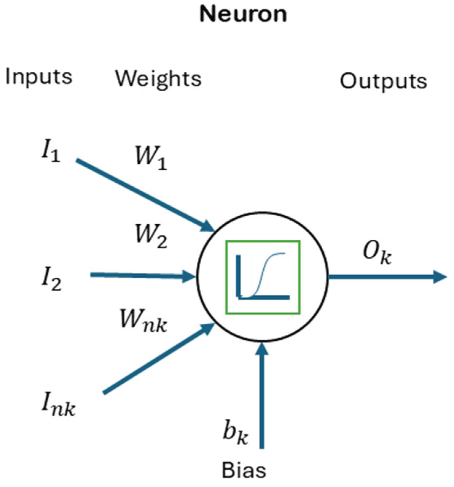
Figure 2.
Feed forward two-hidden-layer neural network.
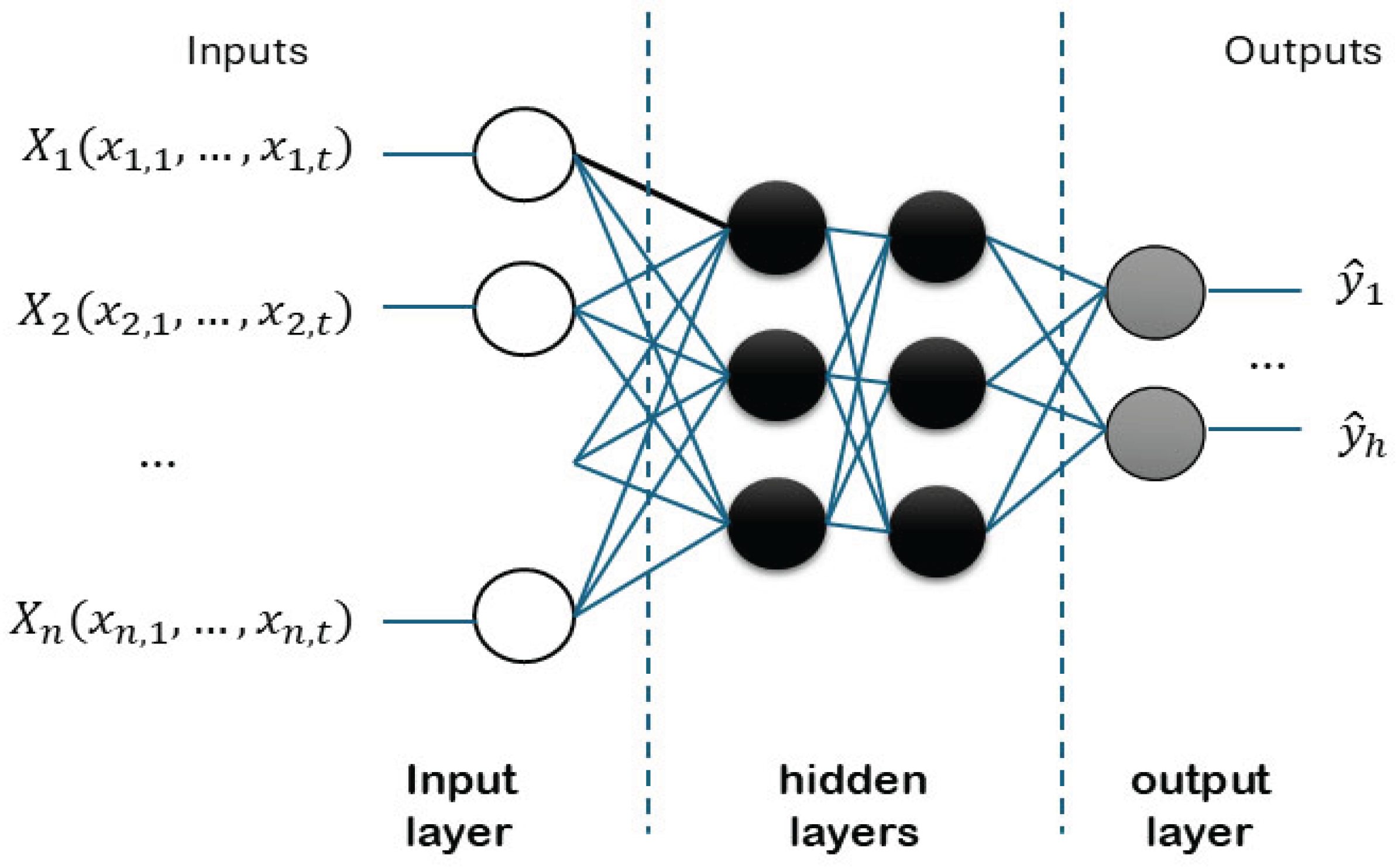
Figure 3.
Schema of a regression tree.
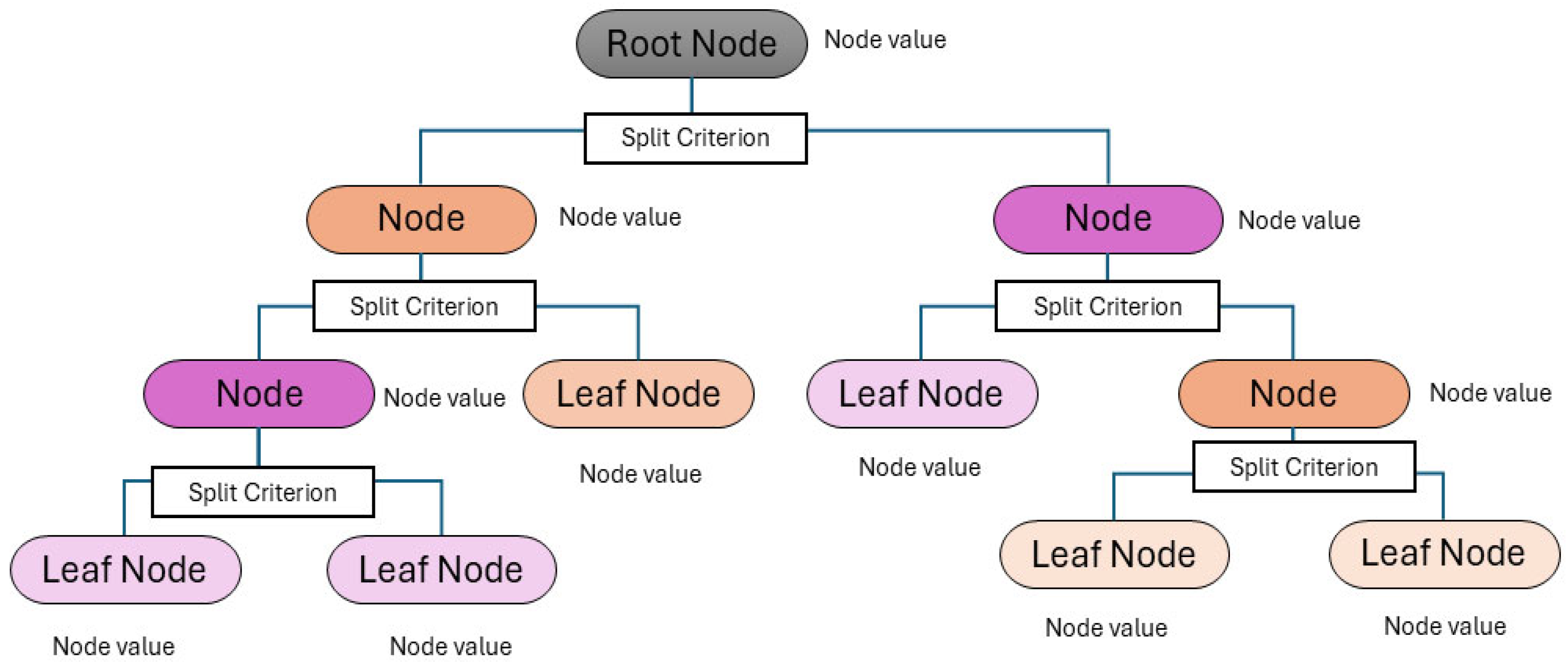
Figure 4.
Schema of a random forest bootstrap aggregation.
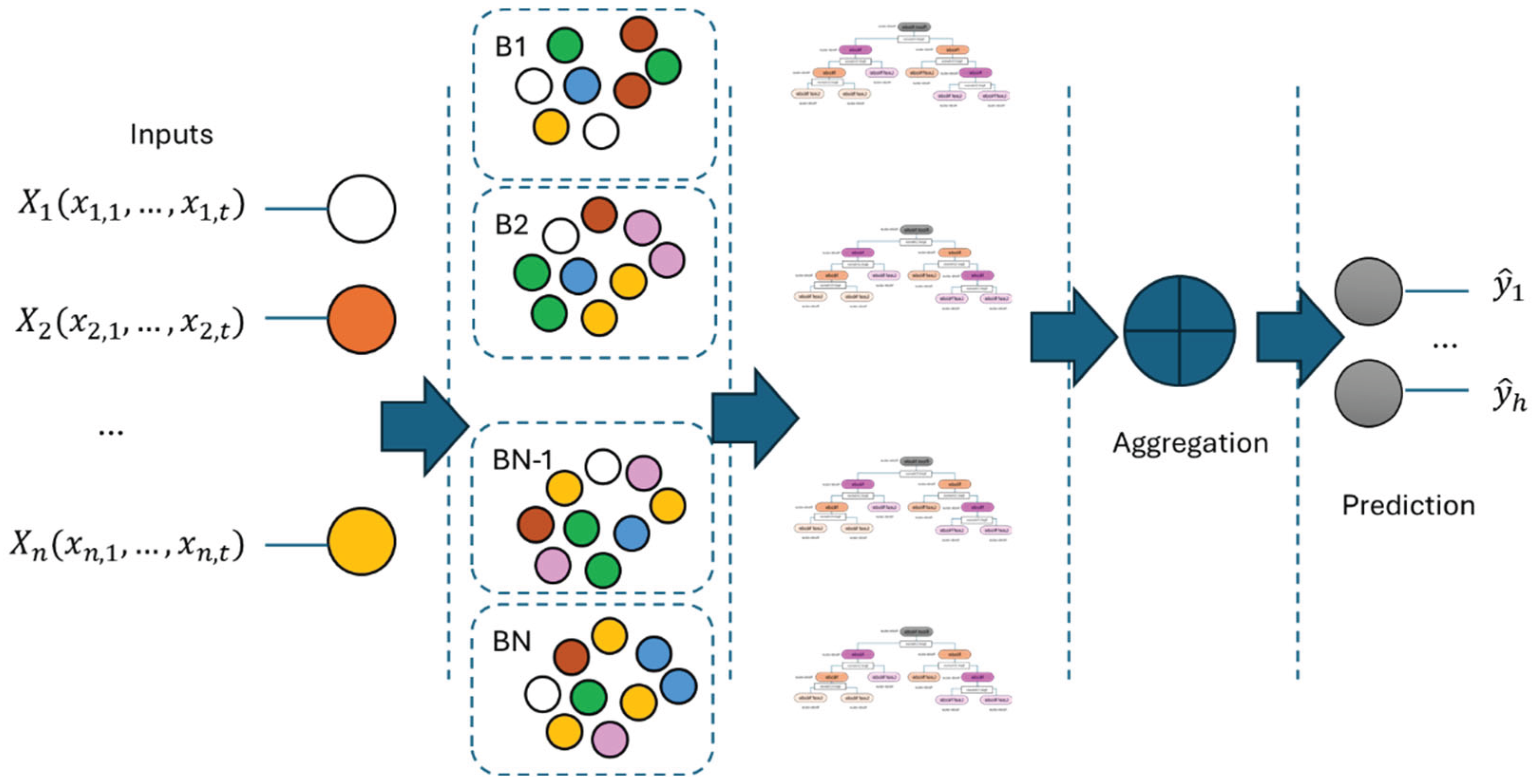

Table 1.
Comparison of global irradiance using statistical methods and machine learning techniques.
| intra-hour | intra-day | day-ahead | ||||||||
|---|---|---|---|---|---|---|---|---|---|---|
| GHI | RMSE | RMSE | RMSE | |||||||
| Statistical methods |
lasso | 68.4 | +/-8.48 | 88.0 | +/-19.58 | 101.1 | +/-53.5 | |||
| lasso + weather | 67.2 | +/-8.15 | 93.1 | +/-22.58 | 70.5 | +/-29.06 | ||||
| ols | 67.7 | +/-8.46 | 89.2 | +/-18.78 | 98.5 | +/-50.79 | ||||
| ols + weather | 66.4 | +/-8.1 | 83.1 | +/-18.77 | 75.1 | +/-33.2 | ||||
| ridge | 68.5 | +/-8.5 | 87.7 | +/-19.34 | 100.5 | +/-52.41 | ||||
| ridge + weather | 67.3 | +/-8.13 | 99.5 | +/-21.15 | 74.1 | +/-32.59 | ||||
| Machine Learning methods |
||||||||||
| Random Forest | 66.8 | +/-8.79 | 86.9 | +/-18.65 | 98.0 | +/-50.54 | ||||
| Random Forest + weather | 63.8 | +/-7.91 | 78.9 | +/-19.75 | 68.6 | +/-31.57 | ||||
| Neural network | 66.3 | +/-9.01 | 91.5 | +/-17.66 | 152.2 | +/-83.38 | ||||
| Neural network + weather | 64.8 | +/-8.41 | 92.9 | +/-18.03 | 107.1 | +/-52.17 | ||||
| Regresion Tree | 81.5 | +/-11.65 | 103.5 | +/-19.65 | 120.6 | +/-63.41 | ||||
| Regression Tree+weather | 81.1 | +/-11.43 | 95.8 | +/-20.53 | 84.0 | +/-39.86 | ||||
Table 2.
Comparison of direct irradiance using statistical methods and machine learning techniques.
| intra-hour | intra-day | day-ahead | |||||||
|---|---|---|---|---|---|---|---|---|---|
| DNI | RMSE | RMSE | RMSE | ||||||
| Statistical methods |
lasso | 130.5 | +/-18.19 | 183.0 | +/-35.69 | 261.4 | +/-65.42 | ||
| lasso + weather | 128.8 | +/-17.88 | 188.9 | +/- 47.72 | 177.7 | +/-20.29 | |||
| ols | 130.1 | +/-18.48 | 189.2 | +/-38.24 | 258.0 | +/-63.29 | |||
| ols + weather | 127.5 | +/-17.61 | 178.1 | +/-38.36 | 184.2 | +/-25.23 | |||
| ridge | 131.5 | +/-18.73 | 182.6 | +/-38.62 | 262.6 | +/-67.48 | |||
| ridge + weather | 128.7 | +/-17.84 | 200.5 | +/-44.78 | 178.5 | +/-21.47 | |||
| Machine Learning methods |
|||||||||
| Random Forest | 129.2 | +/-18.65 | 185.6 | +/-39.39 | 256.2 | +/-63,83 | |||
| Random Forest + weather | 125.0 | +/-17.6 | 172.4 | +/-40.04 | 173.9 | +/-26,68 | |||
| Neural network | 128.2 | +/-18.49 | 194.2 | +/-38.97 | 334.4 | +/-100,98 | |||
| Neural network + weather | 126.1 | +/-18.27 | 202.1 | +/-41.11 | 247.5 | +/-55,3 | |||
| Regresion Tree | 157.6 | +/-24.27 | 220.9 | +/-41.96 | 316.6 | +/-84,14 | |||
| Regresion Tree+ weather | 158.4 | +/-25.69 | 214.8 | +/-45.22 | 211.9 | +/-41,6 | |||
Table 3.
Comparison of Time Series approach methods for global horizontal irradiance.
| Intra-hour | Intra-day | day-ahead | ||||||||
|---|---|---|---|---|---|---|---|---|---|---|
| GHI | RMSE | RMSE | RMSE | |||||||
| TS | Random Forest | 206.9 | +/-74.06 | 214.3 | +/-3.33 | 329.7 | +/-0.67 | |||
| Random Forest + features | 207 | +/-72.84 | 214.3 | +/-3.34 | 329.7 | +/-0.67 | ||||
| Neural network | 207.0 | +/-73.98 | 215.2 | +/-3.39 | 329.6 | +/-0.66 | ||||
| Neural network + feat | 207.0 | +/-74.88 | 214.5 | +/-3.32 | 329.6 | +/-0.66 | ||||
| Regression Tree | 206.9 | +/-91.29 | 215.0 | +/-3.38 | 329.7 | +/-0.67 | ||||
| Regression Tree+features | 206.9 | +/-94.11 | 214.3 | +/-3.34 | 329.7 | +/-0.67 | ||||
| TS | Random Forest | 41.3 | +/-127.13 | 46.3 | +/-1.48 | 82.2 | +/-2.56 | |||
| hybrid | Random Forest + features | 40.7 | +/-125.57 | 45.8 | +/-1.5 | 78.8 | +/-1.8 | |||
| Neural network | 41.1 | +/-0 | 45.6 | +/-1.43 | 74.4 | +/-1.66 | ||||
| Neural network + feat | 41.7 | +/-0 | 46.1 | +/-1.7 | 76.5 | +/-1.82 | ||||
| Regression Tree | 44.9 | +/-0 | 51.0 | +/-1.08 | 90.4 | +/-2.73 | ||||
| Regression Tree+features | 46.0 | +/-0 | 54.8 | +/-2.06 | 92.6 | +/-2.95 | ||||
Table 4.
Comparison of time series approach methods for the direct normal irradiance.
| Intra-hour | Intra-day | day-ahead | ||||||||
|---|---|---|---|---|---|---|---|---|---|---|
| DNI | RMSE | RMSE | RMSE | |||||||
| TS | Random Forest | 260.7 | +/-1.55 | 274.8 | +/-5.09 | 403.6 | +/-1.05 | |||
| Random Forest + features | 260.6 | +/-1.54 | 274.8 | +/-5.09 | 403.5 | +/-1.08 | ||||
| Neural network | 261.3 | +/-1.15 | 275.0 | +/-5.07 | 403.4 | +/-0.98 | ||||
| Neural network + feat | 260.9 | +/-1.56 | 275.0 | +/-5.07 | 403.5 | +/-1.02 | ||||
| Regresion Tree | 261.2 | +/-1.14 | 274.8 | +/-5.09 | 403.5 | +/-1.01 | ||||
| Regression Tree+features | 260.6 | +/-1.54 | 274.8 | +/-5.09 | 403.6 | +/-1.05 | ||||
| TS | Random Forest | 116.9 | +/-2.17 | 128.4 | +/-3.42 | 210.8 | +/-6.58 | |||
| hybrid | Random Forest + features | 113.4 | +/-2.15 | 125.6 | +/-3.49 | 209.0 | +/-7.53 | |||
| Neural network | 116.5 | +/-1.96 | 124.6 | +/-1.33 | 198.9 | +/-7.54 | ||||
| Neural network + feat | 113.4 | +/-2.08 | 124.8 | +/-2.39 | 205.0 | +/-7 | ||||
| Regression Tree | 121.4 | +/-3.76 | 134.6 | +/-1.83 | 225.5 | +/-6.32 | ||||
| Regression Tree+features | 120.2 | +/-4.82 | 140.6 | +/-5.27 | 239.1 | +/-6.28 | ||||
Disclaimer/Publisher’s Note: The statements, opinions and data contained in all publications are solely those of the individual author(s) and contributor(s) and not of MDPI and/or the editor(s). MDPI and/or the editor(s) disclaim responsibility for any injury to people or property resulting from any ideas, methods, instructions or products referred to in the content. |
© 2025 by the authors. Licensee MDPI, Basel, Switzerland. This article is an open access article distributed under the terms and conditions of the Creative Commons Attribution (CC BY) license (http://creativecommons.org/licenses/by/4.0/).
Copyright: This open access article is published under a Creative Commons CC BY 4.0 license, which permit the free download, distribution, and reuse, provided that the author and preprint are cited in any reuse.


