
Submitted:
07 August 2025
Posted:
08 August 2025
You are already at the latest version
Abstract
In this study, a sensorless speed control method is proposed to enhance the speed control performance under load variations by utilizing a discrete–time flux observer in a V/f control environment. Due to their simple structure, low cost, and high reliability, induction motors are widely used in various fields, such as fans, pumps, and home appliances. Among the control methods for induction motors, V/f control operates as an open-loop system, without using speed sensors. It is mainly applied in industrial environments where fast dynamic performance is not required, due to its simple implementation and low cost. However, in cases of load variations or low-speed operation, it suffers from performance degradation and control limitations due to flux variations. To overcome these issues, this paper proposes a method that uses a discrete–time flux observer to estimate the stator flux. We calculate the rotor speed based on the estimated flux, and then improve V/f control performance by adding a compensation signal to the reference frequency, which signal is generated through a PI controller based on the difference between the estimated rotor speed and the reference speed. The proposed method is validated through MATLAB/Simulink-based simulations and experiments using a 5.5 kW induction motor M−G set, confirming that compared to conventional V/f control, the speed maintenance capability and overall robustness against load variations are enhanced. This study presents a practical solution to effectively improve the performance of existing V/f control systems without adding external sensors.
Keywords:
deadbeat observer
; speed control
; flux observer
; induction motor
; V/f control
1. Introduction
Due to their simple structure and low cost, induction motors are widely used in various applications, such as large industrial pumps and water supply systems. They are particularly suitable for driving large-capacity pumps of several hundred kilowatts, thanks to their stable operation, and serve as a core driving source that accounts for a significant portion of industrial motors [1]. Traditionally, induction motors are operated at constant speed; however, maintaining a fixed speed under varying load conditions leads to unnecessary energy losses. In contrast, introducing variable-speed control allows the speed to be adjusted according to the load conditions, thereby improving energy efficiency. In practice, applying inverter-based variable-speed control to loads such as fans, pumps, and blowers can yield significant energy savings [1,2,3,4]. For this reason, interest in variable-speed operation of induction motors continues to increase.
Control methods for induction motors are generally classified into V/f control (scalar control) and vector control. V/f control is an open-loop method that maintains constant motor flux by applying voltage proportional to the supply frequency, offering the advantages of simple structure, with no requirement for sensors. However, V/f control has limitations for precise torque and speed control, as under load variations, slip occurs between the reference and actual speed, resulting in decreased control accuracy. On the other hand, vector control is a closed-loop method that controls the flux and torque components of the motor separately, enabling fast dynamic response and high precision. However, implementing vector control requires speed/position sensors, such as encoders or resolvers, and high-performance microprocessors, which increase system cost and complexity. Although sensorless vector control techniques have been studied to reduce sensor costs and maintenance issues, their speed estimation accuracy decreases with motor parameter variations, while their control algorithms become more complex. For these reasons, V/f control remains widely used in many industrial sites where high-speed response is not required, as it is more cost-effective.
However, since V/f control operates the motor by controlling voltage according to frequency, it faces various performance limitations. When the load torque increases, the slip also increases, preventing the motor from following the reference speed. In addition, during transients, the speed response is slow; and in low-speed regions, the voltage drop that stator resistance causes prevents sufficient flux generation, making stable operation difficult. Various studies have been conducted to overcome performance degradation due to these V/f control limitations, and to secure stable operation [5,6,7,8,9,10,11,12,13,14,15,16].
One representative improvement method to enhance V/f control performance is the voltage boost technique, which compensates for the flux reduction caused by stator resistance at low speeds by adding extra voltage [5,6]. This method stabilizes flux maintenance even in the low-frequency region, by compensating for the voltage drop caused by the winding resistance of the motor. In addition, current-based slip compensation methods have been proposed, which monitor the DC link current of the inverter or the stator current to estimate slip components according to load variations, and apply a compensation frequency proportional to this estimation [2,3,7]. Such simple feedback compensation can be implemented without additional sensors and provides active damping effects, reducing vibrations in light load conditions. When a speed sensor is allowed, it is possible to directly correct the slip by measuring the actual motor speed or implement closed-loop speed control by using a PI controller to compensate the deviation between the reference speed and actual speed [1,8,9,10,11]. While these methods achieve higher accuracy than sensorless systems, the inclusion of speed sensors significantly increases system cost. In a different approach, several studies have attempted to enhance the efficiency of V/f control by integrating Maximum Torque Per Ampere (MTPA) algorithms [12,13]. The MTPA technique operates the motor to generate maximum torque for a given current, thereby reducing losses and improving system efficiency, particularly in partial load conditions. Since the MTPA technique is effective in improving efficiency by maximizing torque per unit current, its direct application in V/f control is challenging due to the scalar nature of V/f control, which does not separately regulate torque and flux components as in vector control frameworks.
Flux observation and compensation methods using induction motor models have also been proposed to improve V/f control performance. Some methods estimate the stator flux using a low-pass filter (LPF), and calculate torque or slip based on the estimated flux to apply feedforward compensation [14,15]. These methods have the advantage of being able to control the motor by simply calculating the flux without sensors, but since they do not continuously correct the estimation through feedback like observers, errors increase if motor parameters differ. In particular, implementing continuous–time flux observers in discrete systems is uncertain. To solve these problems, studies applying discrete–time flux observers, derived by discretizing continuous–time flux observers, have been conducted [16]. This method calculates torque based on the flux estimated by the discrete–time flux observer, and compensates the reference rotor speed using feedforward that is proportional to the calculated torque. However, since this structure does not directly compensate for actual speed errors, speed response vibrations may occur if the gain is large or the torque signal contains large ripples, which limits precise speed control.
To overcome the limitations of such conventional methods, this paper proposes a method that compensates the error between the reference rotor speed and the estimated rotor speed by utilizing a deadbeat discrete–time flux observer. The proposed method estimates the stator flux using the discrete–time flux observer, and calculates the slip speed and rotor speed in real time based on the estimated flux. The difference between the calculated rotor speed and the reference rotor speed is compensated through a PI controller, and the resulting compensation signal is added to the reference rotor speed to correct slip caused by load variations. As a result, improved speed response and load robustness compared to the conventional V/f control and torque feedforward compensation methods have been achieved. The effectiveness of the proposed method is verified through MATLAB/Simulink-based simulations and experiments using a 5.5 kW induction motor M−G set, confirming the improved speed control performance.
2. Structure and Mathematical Modeling of the Induction Motor
2.1. Structure and Characteristics of the Induction Motor
An induction motor is an electromechanical device, consisting of a stator and a rotor, that converts electrical energy into mechanical energy. In the case of a three-phase squirrel-cage induction motor, which is widely used in industrial applications, the stator is composed of symmetrical three-phase windings, while the rotor is made of conductive bars. When a three-phase alternating current is applied to the stator, a rotating magnetic field is generated, which induces current in the rotor conductors. The interaction between the induced current and the rotating magnetic field causes the rotor to rotate.
Induction motors have advantages of simple and robust structure, ease of maintenance, and low cost. These characteristics lead to them being widely used in various fields, such as industrial fans, large pumps, and water supply systems, and they are capable of stable operation even in high-power systems above 100 kW. However, unlike synchronous machines, the rotor speed of an induction motor is always lower than the synchronous speed; this difference is referred to as slip. While slip is an essential factor in the operating principle of induction motors, it also becomes a cause of difficulty in achieving precise speed control. In particular, near zero speed, it becomes challenging to accurately estimate the rotor speed or position using sensorless methods, as the induced voltage and flux variation become very small. As a result, induction motors have limitations in precise position control and stable control during the initial start-up phase.
2.2. Mathematical Modeling of the Induction Motor
For a basic 3-phase induction motor, Eqs. (1) & (2) give the voltage equations of the stator and rotor circuits, respectively, while Eq. (3) gives the stator and rotor flux linkages [17]:
where, , , and represent the three-phase voltage, current, and flux linkage, respectively, where the subscripts and denote the stator and rotor, respectively, while and represent the conductor resistance, inductance, and mutual inductance components, respectively, and denotes differentiation.
In the three-phase coordinate system, the voltage equations contain time-varying components, which make it complicated to analyze the characteristics of the induction motor. Therefore, by applying coordinate transformation, the three-phase variables can be converted into a two-axis coordinate system to obtain constant components, making it easier to analyze the dynamic characteristics. Coordinate transformation can be performed either using a stationary reference frame, based on the stator, or a synchronously rotating reference frame, based on the rotor rotating at synchronous speed. In this study, the three-phase coordinates are converted to a stationary reference frame to implement the discrete–time flux observer.
In the stationary reference frame, the d-axis is aligned with the a-phase of the stator, and the q-axis leads the d-axis by 90°. By applying the Clarke transformation to convert the coordinate system, the stator voltage equations and flux linkages of the induction motor in the stationary reference frame are expressed as Eqs. (4)–(6):
where, , , , , , and represent the respective d–q axis voltage, current, and flux linkage in the stationary reference frame, while and represent the stator leakage inductance and magnetizing inductance, respectively, and represents the angular speed of the coordinate system, while in the transformed equations, there are speed voltage terms expressed as and [8]. However, since the stationary reference frame does not rotate, is zero.
Equation (7) gives the stator voltage equations in the stationary reference frame, while Eqs. (8) and (9) can construct the mathematical model of the three-phase induction motor [18]:
where, , , and represent the voltage, current, and flux linkage, respectively, in the stationary reference frame, while, , , , , , , , , and represent the relevant parameters of the motor model.
3. Proposed Speed Control Method for Induction Motor
In this study, a discrete–time flux observer is designed to estimate the rotor slip speed in real time, and robust and fast speed control performance is achieved in V/f control through feedback compensation using the estimated speed, even under load variations.
3.1. Continuous–Time Flux Observer
Considering that the system matrix A in the mathematical model of Eq. (8) varies according to the speed component, a full-order Luenberger observer in the stationary reference frame can be constructed, as shown in Eq. (10) [19]. The constructed observer can robustly estimate the stator flux, even under parameter variations [18]. Figure 1 illustrates the dominant poles of the original motor system and the observer-based system, which vary according to rotor speed. Regardless of speed, the poles of the observer system remain stably located in the left-half plane, ensuring consistent system stability and faster dynamic response, compared to the original system.
In the case of Eq. (8), since the system matrix A contains speed components, the poles shift, depending on the speed; this characteristic is represented by the red region in Figure 1. At low speeds, the poles are located near the origin; but as the speed increases, the poles move along the real axis into the left-half plane. Therefore, at low speeds, the poles are closer to the imaginary axis, which can result in larger errors due to slow control response.
Similarly, in the case of Eq. (10), both the speed-dependent components of the A matrix and the variations in the observer feedback gain K cause the poles to shift further from the origin into the left-half plane. As indicated by the blue region in Figure 1, the poles remain within the stable region, regardless of speed. Thus, by constructing a full-order Luenberger observer, stable estimation and control can be achieved across the entire operating range. Using the constructed flux observer, direct torque control or slip/torque components can be utilized to improve speed control performance [14,15,21,22].
where, ^ is the estimated state, ,and .
3.2. Discrete Flux Observer
Since the continuous–time flux observer cannot be directly applied in discrete control, a discretization process is necessary. To accurately analyze the system in discrete time, the continuous–time mathematical model in Eq. (8) can be transformed into Eqs. (14) and (15) through the relations in Eqs. (11)–(13) [20]:
where, is the sampling time of the discrete system, and , , and represent the discretized values of , , and , respectively. For the discrete–time system described in Eqs. (14) and (15), the observer can be constructed as shown in Eq. (16):
where, K is the observer feedback gain, and denotes the estimated state at time calculated based on the state at time .
To achieve fast observer performance in discrete time, a deadbeat observer is applied. In a deadbeat observer, all characteristic roots of the observer error dynamics are placed at the origin by adjusting K in Eq. (16). The deadbeat observer has the characteristic of driving the observer error to zero within a finite time. Therefore, although the observer feedback gain becomes very large, fast observation performance can be expected. The observer feedback gain for the deadbeat observer can be calculated using Ackermann’s formula, as expressed in Eq. (17). Furthermore, placing all poles at the origin simplifies the characteristic equation of the matrix, as shown in Eq. (18), and based on the Cayley-Hamilton theorem, Eq. (19) holds [20]:
where, P is the characteristic polynomial, is the observability matrix, and n is the system order.
Figure 2 shows that all poles of the closed-loop system with the deadbeat observer are located inside the unit circle, ensuring system stability. Moreover, since the poles are concentrated at the origin, a fast system response can be expected:
3.3. Discrete Flux Observer Using Reference Rotor Speed
In this study, the flux observer is designed as a deadbeat observer based on the mathematical model given in Eq. (8). As shown in Figure 19 and Figure 20 of the reference materials, the matrices , , and , which vary with the rotor speed , exhibit only slight variations in most elements, except for certain components of the matrix in the low-speed region. Therefore, even when using the reference rotor speed instead of the actual rotor speed, it has little effect on the stator flux estimation performance or speed control. In addition, since each matrix element can be expressed as a combination of second-order, third-order, or exponential functions, a lookup table can be constructed to reduce computation time. Alternatively, matrix variations according to speed can be represented using functional expressions, enabling a simplified observer structure. However, to suppress oscillatory components caused by large observer gains at low speeds, a constant speed value is applied in the low-speed region to ensure stable observer operation.
3.4. The Proposed Sensorless Speed Control Method
The stator flux estimated by the flux observer in the stationary reference frame can be transformed into the rotor flux in the stationary reference frame using Eqs. (20) and (21):
where, and in the stationary reference frame determine the direction of the rotor flux. Based on these values, the flux angle can be calculated using Eq. (22):
The flux angle serves as the reference to convert variables from stationary reference frame to rotating reference frame. Using this angle, the stator current in the stationary reference frame can be transformed into the rotating reference frame, as shown in Eq. (23):
By using the q–axis current component in the rotating reference frame, the stator flux in the rotating reference frame can be calculated as follows:
Finally, the slip speed can be calculated using the results of Eqs. (23) and (24), as shown in Eq. (25). The estimated rotor speed is then obtained by subtracting the slip speed from the reference speed , as expressed in Eq. (26):
The speed error is calculated using Eq. (27), and this error is passed through a PI controller. The output of the PI controller is then added to the reference speed for compensation, as shown in Eq. (28):
where, is the compensated reference speed, is the proportional gain, and is the integral gain.
4. Simulation Configuration and Results
4.1. Simulation Configuration
Figure 3 illustrates the structure of the MATLAB/Simulink-based simulator designed to validate the effectiveness of the proposed sensorless speed estimation method using a deadbeat discrete–time flux observer. The simulator is configured by adding a speed estimation and compensation path, based on the deadbeat discrete–time flux observer, to a conventional V/f control scheme. The entire system operates under a fixed-step simulation environment. The control loop for V/f control is executed at a sampling period of 1 ms, while to ensure rapid dynamic response, the flux observer and speed estimation algorithms are computed at a faster rate of 0.1 ms. The inverter is driven using the space vector pulse width modulation (SVPWM) technique, with a switching frequency set to 5 kHz. The measured three-phase stator voltages and currents are transformed into the stationary reference frame (α–β frame) via the Clarke transformation, and the resulting components are used as inputs to the flux observer. The rotor flux is computed from the estimated stator flux, and the flux angle is estimated to transform the flux and current into the rotating reference frame (d–q frame). Using these d–q frame quantities, the slip speed and rotor speed are calculated in real time. The difference between the calculated rotor speed and the reference speed is processed through a PI controller, and the output is added to the reference rotor speed to actively compensate for slip caused by load variations. The Runge–Kutta method is applied for numerical integration. Table 1 summarizes the key parameters of the induction motor used in both the simulation and experimental validation.
4.2. Simulation Results
To evaluate the performance of the proposed sensorless speed estimation method based on the deadbeat discrete–time flux observer, simulations were conducted under (30 and 50) % rated load conditions, focusing on its compensation capability. In the simulation, the rotor speed was linearly accelerated to 2,400 rpm over the initial 4 s, and maintained at the target speed for the following 20 s. After 24 s, either (30 or 50) % of the rated load was applied to analyze the difference between the actual and estimated speeds. Subsequently, to verify the effectiveness of the sensorless speed control using the estimated speed, the same reference rotor speed was maintained while applying (30 and 50) % rated loads. The results of the proposed control method were compared with those of conventional open-loop V/f control and the existing torque feedforward compensation method.
Figure 4 presents the simulation results under the 30 % rated load condition. Figure 4a shows the rotor speed and load torque responses over the entire simulation duration, while Figure 4b highlights the transient behavior of the speed and torque after the load is applied in the steady state. In the figures, the green, blue, red, and black lines represent the reference rotor speed, actual rotor speed, estimated rotor speed, and load torque, respectively. The results confirm that throughout the simulation, the estimated speed closely tracks the actual rotor speed. Notably, even after the 30 % load is applied, the proposed method maintains stable and accurate speed estimation performance.
Figure 5 shows the simulation results of the speed control performance under a 30 % rated load condition. Figure 5a presents the system response in steady-state operation, while Figure 5b illustrates the speed error with respect to the reference speed. In the figures, the green, red, blue, purple, and black lines denote the reference speed, proposed speed control method, conventional open-loop V/f control, conventional torque feedforward compensation method, and load torque, respectively. Under the 30 % rated load condition, the conventional open-loop V/f control results in a speed drop to 2,383.17 rpm, with an average speed error of 16.83 rpm and an error rate of 0.7 %. The conventional torque feedforward compensation method slightly improves the result, achieving 2,389.65 rpm with an average speed error of 10.35 rpm and an error rate of 0.43 %. In contrast, the proposed sensorless speed control method achieves a speed of 2,399.69 rpm, yielding an average speed error of only 0.31 rpm, and an error rate of 0.01 %. These results clearly demonstrate the superior speed tracking performance of the proposed method, maintaining rotor speed closer to the reference value, even under load variations.
Figure 6 presents the simulation results under the condition where 50 % of the rated load is applied. Figure 6a shows the rotor speed and torque responses over the entire simulation period, while Figure 6b illustrates the responses when the 50 % load is applied during steady-state operation. Despite the increase in load from (30 to 50) %, the difference between the actual and estimated rotor speeds remains minimal, indicating that the proposed speed estimation method maintains stable performance, even under significant load variations.
Figure 7 shows the simulation results of the speed control performance under a 50 % rated load condition. Figure 7a presents the system response in steady-state operation, while Figure 7b illustrates the speed error with respect to the reference speed. When using conventional open-loop V/f control, the rotor speed drops to 2,371.56 rpm under 50 % load, resulting in an average speed error of 28.44 rpm and an error rate of 1.19 %. The conventional torque feedforward compensation method slightly improves the performance, achieving 2,382.43 rpm with an average speed error of 17.57 rpm and an error rate of 0.73 %. In contrast, the proposed sensorless speed control method maintains the rotor speed at 2,399.44 rpm, with an average speed error of only 0.56 rpm and an error rate of 0.02 %. These results confirm that the proposed method provides significantly improved speed tracking accuracy, keeping the rotor speed much closer to the reference, even under heavier load conditions.
The sensorless speed estimation method using the deadbeat discrete–time flux observer demonstrated stable performance under both (30 and 50) % rated load conditions, maintaining a steady-state speed error within the range (0.5 to 1) rpm between the actual and estimated speeds. These results indicate that the proposed estimation method is robust against load variations. In consequence, the proposed speed control method showed improved performance compared to the conventional open-loop V/f control and the existing torque feedforward compensation method. Table 2 summarizes the results:
5. Experimental Configuration and Results
5.1. Experimental Configuration
Figure 8 illustrates the experimental setup used to validate the effectiveness of the proposed sensorless speed control method based on the deadbeat discrete–time flux observer. Figure 8a shows the M−G set employed in the experiments. Both motors are identical 5.5 kW induction motors, with the left motor serving as the load, and the right motor connected to the control system. The two motors are mechanically coupled, and a speed/torque sensor is installed between them. The torque sensor is used to monitor the applied load, while the speed sensor is used to compare the actual rotor speed with the estimated speed. Figure 8b presents the configuration of the control system used in the experiment. The controller generates the reference voltage corresponding to the reference synchronous speed, and produces IGBT switching signals using space vector PWM (SVPWM). These signals are applied to the induction motor through a power module. Based on the measured stator currents and reference voltage, the stator flux is estimated using a flux observer in the stationary reference frame. The rotor flux is calculated from the estimated stator flux, and the flux angle is derived to transform the stator current and flux into the rotating reference frame. The rotor speed is then estimated and controlled using the flux and current in the rotating frame. The control sampling periods are identical to those used in the simulation: 1 ms for the V/f control loop, 0.1 ms for the discrete–time flux observer and feedforward compensation, and a 5 kHz switching frequency for SVPWM. The rotor speed, torque, control variables, and three-phase stator currents can be monitored using the Speed/Torque Display and the easyDSP interface, while an oscilloscope is used for real–time signal observation and data recording:
5.2. Experimental Results
The experiment was conducted under the same reference speed and load conditions as the simulation. The motor was accelerated to the reference speed over 4 s, and the load was applied after 20 s to compare the actual rotor speed with the estimated speed.
Figure 9 shows the experimental results under a 30 % rated load condition. Figure 9a presents the rotor speed and torque responses over the entire experiment duration, while Figure 9b illustrates the responses after applying the 30 % rated load. Figure 9c and d show the estimated stator flux and the three-phase stator currents, respectively. In Figure 9a,b, the green, blue, red, and black lines denote the reference rotor speed, actual rotor speed, estimated rotor speed, and load torque, respectively. Figure 9a shows that throughout the entire experiment, the estimated speed closely follows the actual speed. Figure 9b and c confirm that both speed and flux are estimated stably, even during abrupt load changes. In addition, Figure 9c,d illustrate the transient behavior of the estimated flux and the three-phase stator currents in response to the sudden load variation.
Figure 10 presents the experimental results of the speed control performance under a 30 % rated load condition. In Figure 10a,b, the green, red, blue, purple, and black lines denote the reference speed, proposed sensorless speed control method, conventional open-loop V/f control, conventional torque feedforward compensation method, and load torque, respectively. Figure 10a,b demonstrate the speed control performance of each method, while Figure 10c,d confirm that flux estimation and control remain stable, even under abrupt load changes. As a result, when the load is applied, the conventional open-loop V/f control exhibits a speed drop to 2,373.75 rpm, yielding an average speed error of 26.25 rpm and an error rate of 1.09 %. The conventional torque feedforward compensation method achieves 2,382.75 rpm, with an average speed error of 17.25 rpm and an error rate of 0.72 %, showing slight improvement over the open-loop method. In contrast, the proposed sensorless speed control method maintains a rotor speed of 2,401.12 rpm, resulting in an average speed error of only 1.12 rpm and an error rate of 0.05 %, demonstrating significantly superior speed tracking accuracy, and closer adherence to the reference speed.
Figure 11 presents the experimental results under a 50 % rated load condition. Figure 11a shows the rotor speed and torque responses over the entire experiment duration, while Figure 11b illustrates the steady-state responses of rotor speed and torque. Figure 11c and d display the estimated stator flux and the three-phase stator currents, respectively. Even under a more abrupt load change from (30 to 50) %, the proposed method continues to provide stable estimation of both rotor speed and stator flux:
Figure 12 shows the experimental results of the speed control performance under a 50 % rated load condition. In the case of the conventional open-loop V/f control, the rotor speed drops to 2,360.25 rpm when the load is applied, resulting in an average speed error of 39.75 rpm and an error rate of 1.66 %. The conventional torque feedforward compensation method improves the result to 2,376.75 rpm, with an average speed error of 23.25 rpm and an error rate of 0.97 %, showing slightly better performance than the open-loop method. In contrast, the proposed sensorless speed control method achieves a rotor speed of 2,401.50 rpm, with an average speed error of only 1.50 rpm and an error rate of 0.06 %, demonstrating significantly improved speed tracking performance, and much closer adherence to the reference speed.
The sensorless speed estimation method using the deadbeat discrete–time flux observer demonstrated stable performance under both (30 and 50) % rated load conditions, maintaining a steady-state speed error within 8 rpm, despite load variations. As a result, when compared to the conventional open-loop V/f control and the existing torque feedforward compensation method, the proposed speed control method showed improved performance. Table 3 summarizes the results:
6. Conclusion
This study proposed a sensorless speed control method to compensate for speed deviations caused by load variations in an induction motor system under V/f control. The proposed approach utilizes a deadbeat discrete–time flux observer, which is derived by discretizing a continuous–time model, to estimate the stator flux. Based on the estimated flux, the slip speed and rotor speed are calculated in real time. The difference between the calculated rotor speed and the reference speed is compensated by a PI controller, enabling active slip compensation under varying load conditions.
The effectiveness of the proposed method was validated through both MATLAB/Simulink-based simulations, and experiments using a 5.5 kW induction motor in an M−G set configuration. The experimental results show that compared to the conventional open-loop V/f control and torque feedforward compensation methods, the proposed method provides superior control performance. Specifically, under 50 % of rated load, the speed error of the conventional method was 0.97 %, whereas the proposed method achieved a significantly reduced error of 0.06 %, demonstrating approximately 16 times higher accuracy.
Future research is anticipated to focus on incorporating parameter estimation techniques, such as rotor time constant adaptation, to further enhance the robustness and reliability of the sensorless control system.
References
- Bose, B. K., “Modern Power Electronics and AC Drives,” Prentice Hall PTR, 2002.
- Trzynadlowski, Andrzej M., “Control of induction motors,” Elsevier, 2000.
- Sul, Seung-Ki., “Control of electric machine drive systems,” John Wiley & Sons, 2011.
- Fitzgerald, Arthur Eugene, Charles Kingsley, and Stephen D. Umans. “Fitzgerald & Kingsley's electric machinery,” McGraw-Hill Companies, 2013.
- Francis, C. J., & Zelaya De La Parra, H., “Stator resistance voltage-drop compensation for open-loop AC drives,” IEE Proceedings-Electric Power Applications, vol. 144, no. 1, pp.21-26, 1997.
- Shin, Myoung-Ho, “A Study on Scalar Control of a Synchronous Motor Considering Stator Resistance,” The Transactions of the Korean Institute of Electrical Engineers, vol. 73, no. 9, pp.1545-1550, 2024.
- Smith, A., Gadoue, S., Armstrong, M., & Finch, J., “Improved method for the scalar control of induction motor drives,” IET electric power applications, vol. 7, no. 6, pp.487-498, 2013.
- Kim, Sang-Hoon., “Electric motor control: DC, AC, and BLDC motors,” Elsevier, 2017.
- Reddy, S. R. P., & Loganathan, U., “Robust and high-dynamic-performance control of induction motor drive using transient vector estimator,” IEEE Transactions on Industrial Electronics, vol. 66, no. 10, pp.7529-7538, 2018.
- Shaltout, A., and O. E. M. Youssef., “Speed control of induction motors using proposed closed loop Volts/hertz control scheme,” 2017 Nineteenth International Middle East Power Systems Conference (MEPCON). IEEE, pp.533-537, 2017.
- Jeong, Gang-Youl, “Stability Improvement of a V/f Controlled Induction Motor Drive System using a Dynamic Current Compensator,” The Transactions of the Korean Institute of Electrical Engineers B, vol. 53, no. 6, pp.402-408, 2004.
- Das, T. S., & Roykumar, M, “Maximum Torque per Ampere Controller for 3-Phase Scalar Controlled Induction Motor Drive,” In 2022 International Conference on Intelligent Innovations in Engineering and Technology (ICIIET), IEEE, pp.216-221, 2022.
- Lee, K., & Han, Y., “Reactive-power-based robust MTPA control for v/f scalar-controlled induction motor drives,” IEEE Transactions on Industrial Electronics, vol. 69, no.1, pp.169-178, 2022.
- Luo, H., Wang, Q., Deng, X., Wan, S., “A novel V/f scalar controlled induction motor drives with compensation based on decoupled stator current,” 2006 IEEE International Conference on Industrial Technology, IEEE., pp. 1989-1994, 2006.
- Wang, C. C., Fang, C. H., “Sensorless scalar-controlled induction motor drives with modified flux observer.” IEEE transactions on energy conversion, vol. 18, no. 2, pp.181-186, 2003.
- Hong, Chang-Wan., “Torque Feed-Forward Compensation Method with Discrete Flux Observers for Induction Motor V/f Control”, The Transactions of the Korean Institute of Electrical Engineers, vol. 74, no. 3, pp.455-467, 2025.
- Krause, Paul C., “Analysis of electric machinery and drive systems,” New York: IEEE press, pp.216-220, 2002.
- Vas, Peter., “Sensorless vector and direct torque control,” Oxford university press, 1998.
- Pimkumwong, Narongrit, Ming-Shyan Wang, “Full-order observer for direct torque control of induction motor based on constant V/F control technique,” ISA transactions, vol. 73, pp.189-200, 2018.
- Astrom, K. J., Wittenmark, B., “Computer-controlled systems: theory and design. Courier Corporation,” 2013.
- XUE, Yanhong, “A stator flux-oriented voltage source variable-speed drive based on dc link measurement,” IEEE transactions on industry applications, vol. 27, no. 5, pp.962-969, 1991.
- Li, Yong, Wenxin Huang, and Yuwen Hu., “A low cost implementation of stator-flux-oriented induction motor drive,” International Conference on Electrical Machines and Systems. IEEE, vol. 2, 2005.
- Son, D. H., & Kim, S. A., “Simplified V/f Control Algorithm for Reduction of Current Fluctuations in Variable-Speed Operation of Induction Motors,” Energies, vol. 17, no. 7 : 1699, 2024.
- Carbone, L., Cosso, S., Kumar, K., Marchesoni, M., Passalacqua, M., & Vaccaro, L. Stability analysis of open-loop V/Hz controlled asynchronous machines and two novel mitigation strategies for oscillations suppression. Energies, vol. 15, no. 4 : 1404, 2022.
Figure 1.
Dominant poles of a continuous time motor system with rotor speed variation.
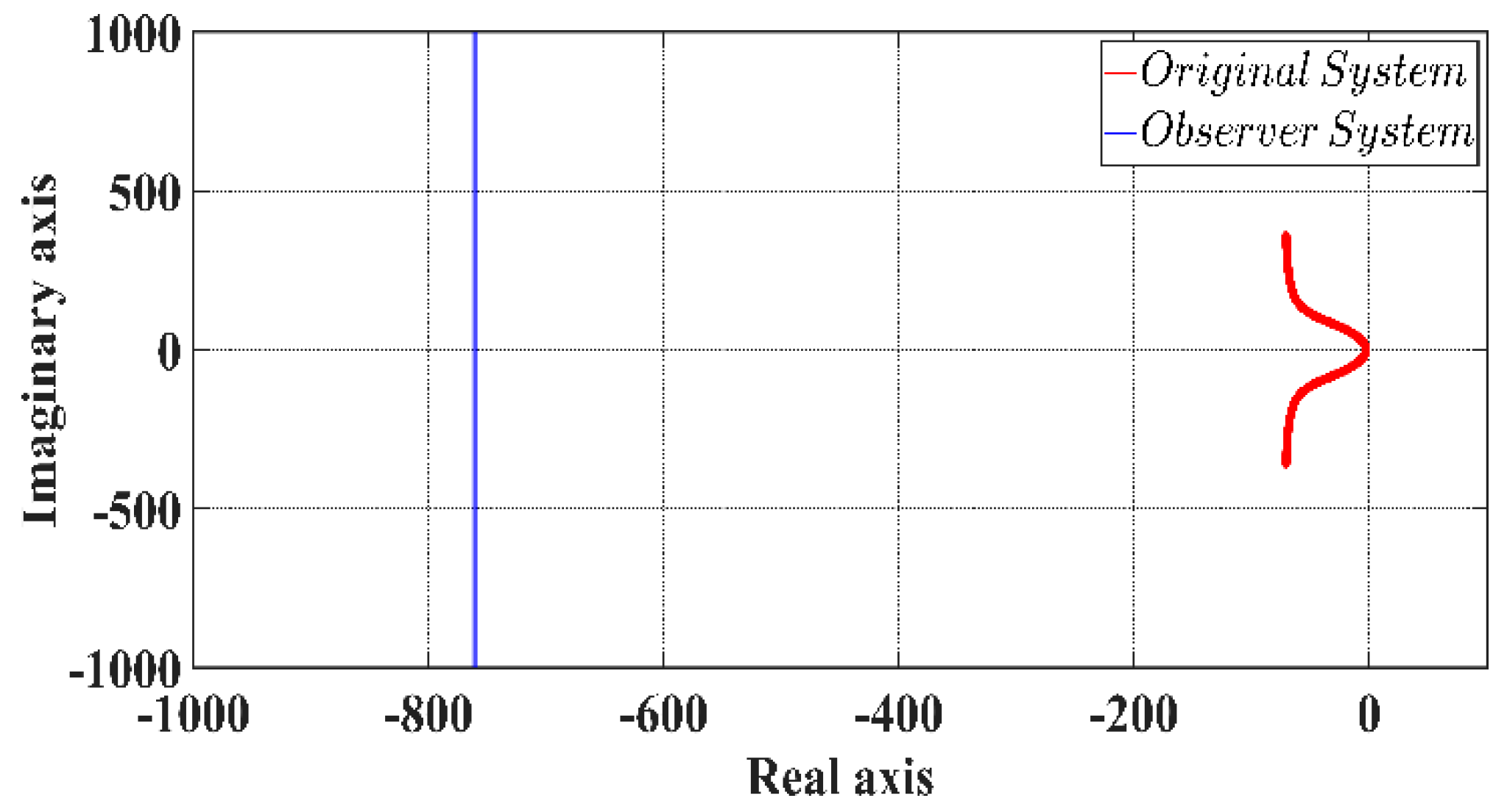
Figure 2.
Poles of a system with deadbeat observers.
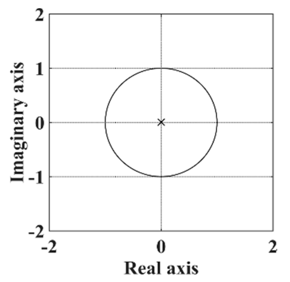
Figure 3.
Simulator Configuration Diagram for Simulations.
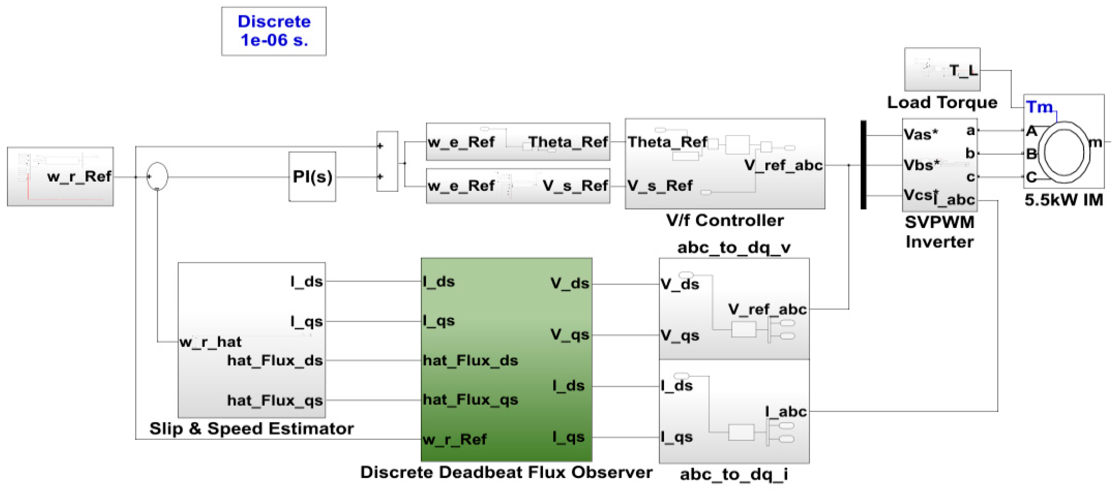
Figure 4.
Speed and torque response at 30 % rated load torque in simulation: (a) Overall, and (b) Steady-state.
Figure 4.
Speed and torque response at 30 % rated load torque in simulation: (a) Overall, and (b) Steady-state.
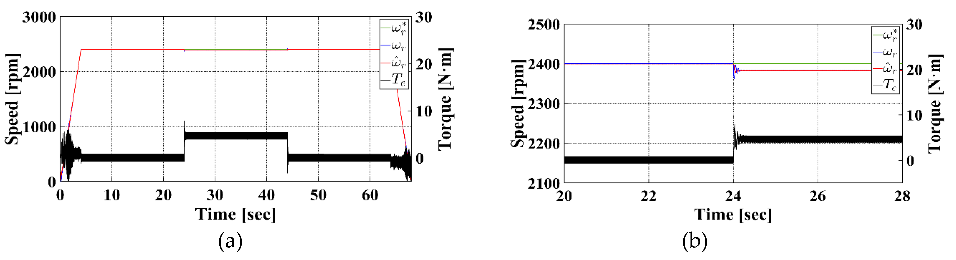
Figure 5.
Speed control result at 30 % rated load torque in simulation: (a) Steady-state, and (b) Speed error with reference speed.
Figure 5.
Speed control result at 30 % rated load torque in simulation: (a) Steady-state, and (b) Speed error with reference speed.
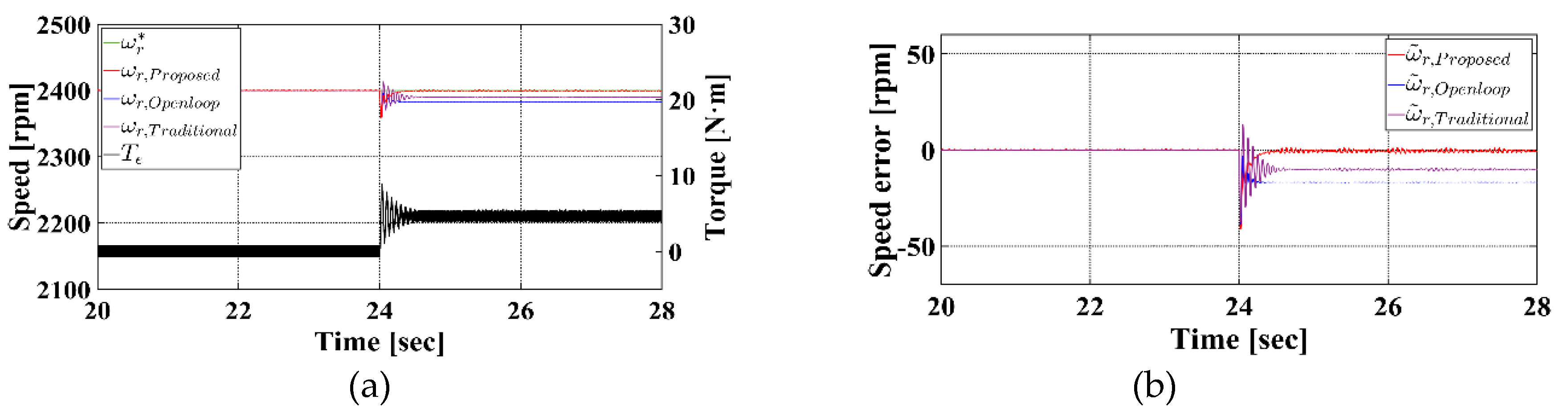
Figure 6.
Speed and torque response at 50 % rated load torque in simulation: (a) Overall, and (b) steady-state.
Figure 6.
Speed and torque response at 50 % rated load torque in simulation: (a) Overall, and (b) steady-state.
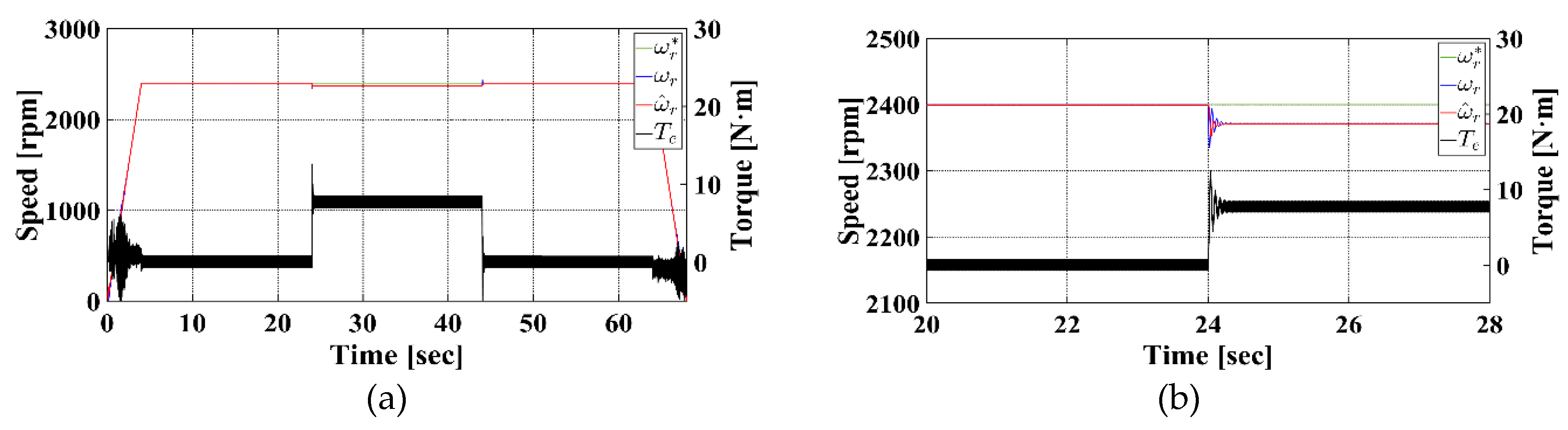
Figure 7.
Speed control result at 50 % rated load torque in simulation: (a) Steady-state, and (b) Speed error with reference speed.
Figure 7.
Speed control result at 50 % rated load torque in simulation: (a) Steady-state, and (b) Speed error with reference speed.
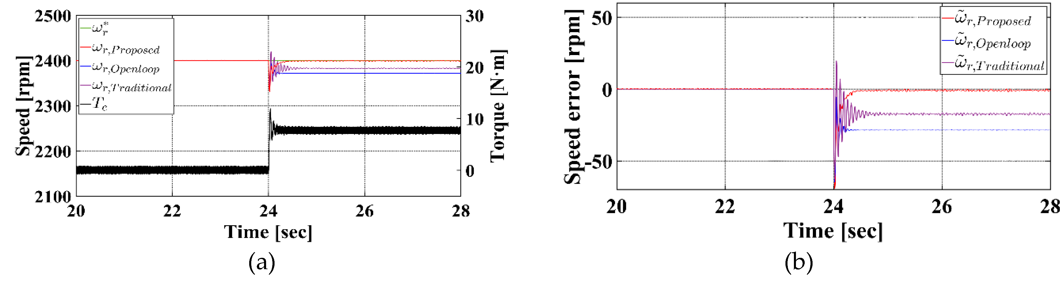
Figure 8.
Configuration of the equipment for the experiment: (a) M−G Set, and (b) Control System.
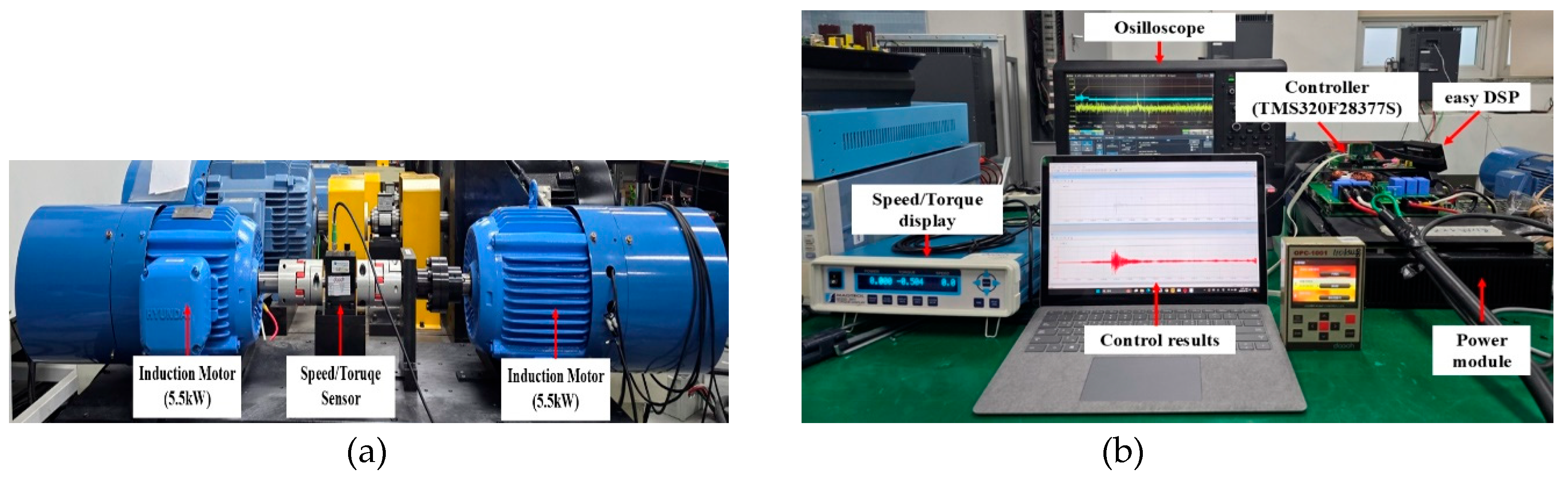
Figure 9.
Experiment result at 30 % rated load (a) Overall, (b) Steady-state, (c) Estimated flux, and (d) Three-phase current.
Figure 9.
Experiment result at 30 % rated load (a) Overall, (b) Steady-state, (c) Estimated flux, and (d) Three-phase current.
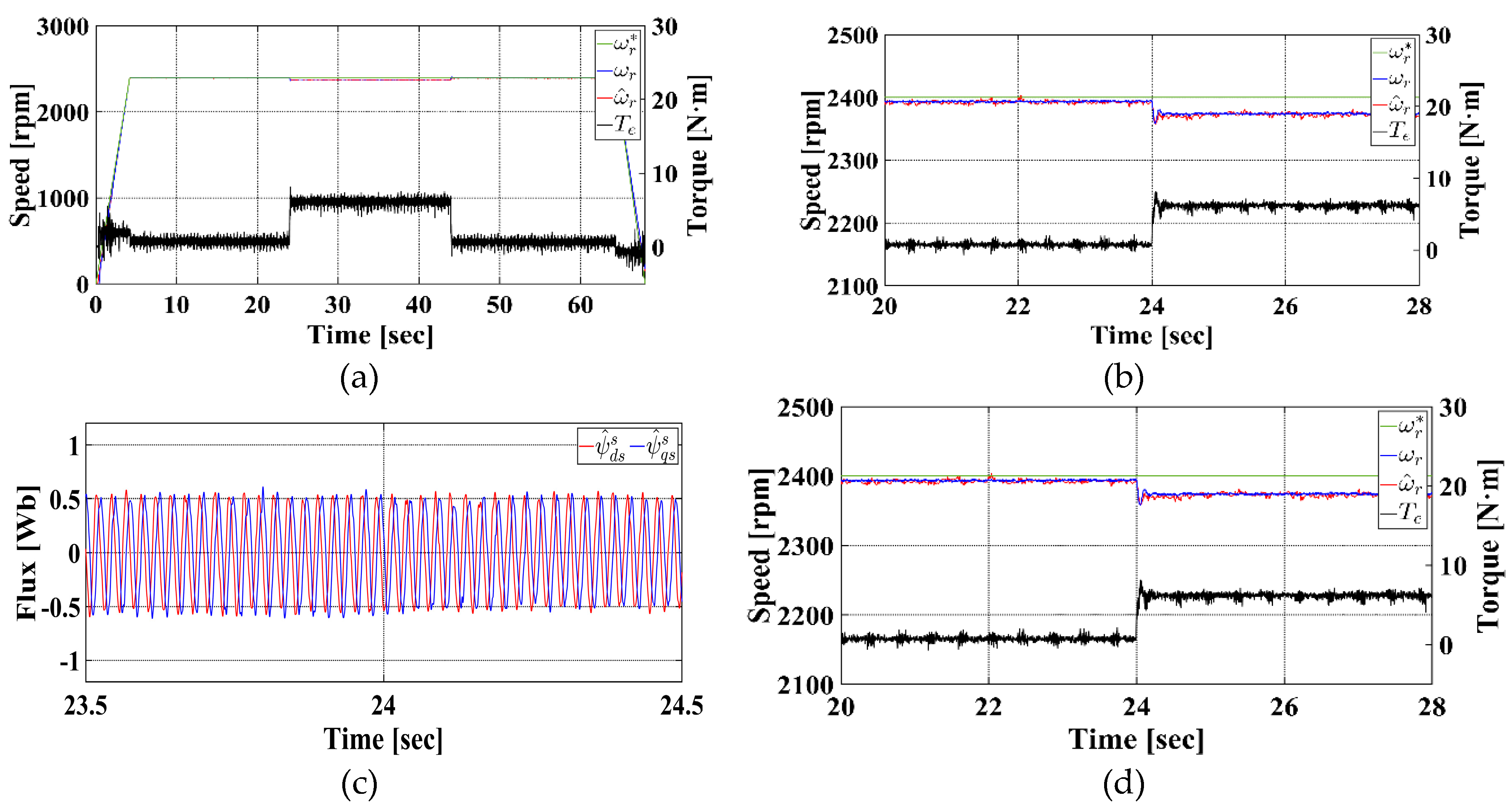
Figure 10.
Speed control result at 30 % rated load torque in experiment: (a) Speed comparison at steady state, (b) Speed error with reference speed, (c) Estimated flux, and (d) Three-phase current.
Figure 10.
Speed control result at 30 % rated load torque in experiment: (a) Speed comparison at steady state, (b) Speed error with reference speed, (c) Estimated flux, and (d) Three-phase current.
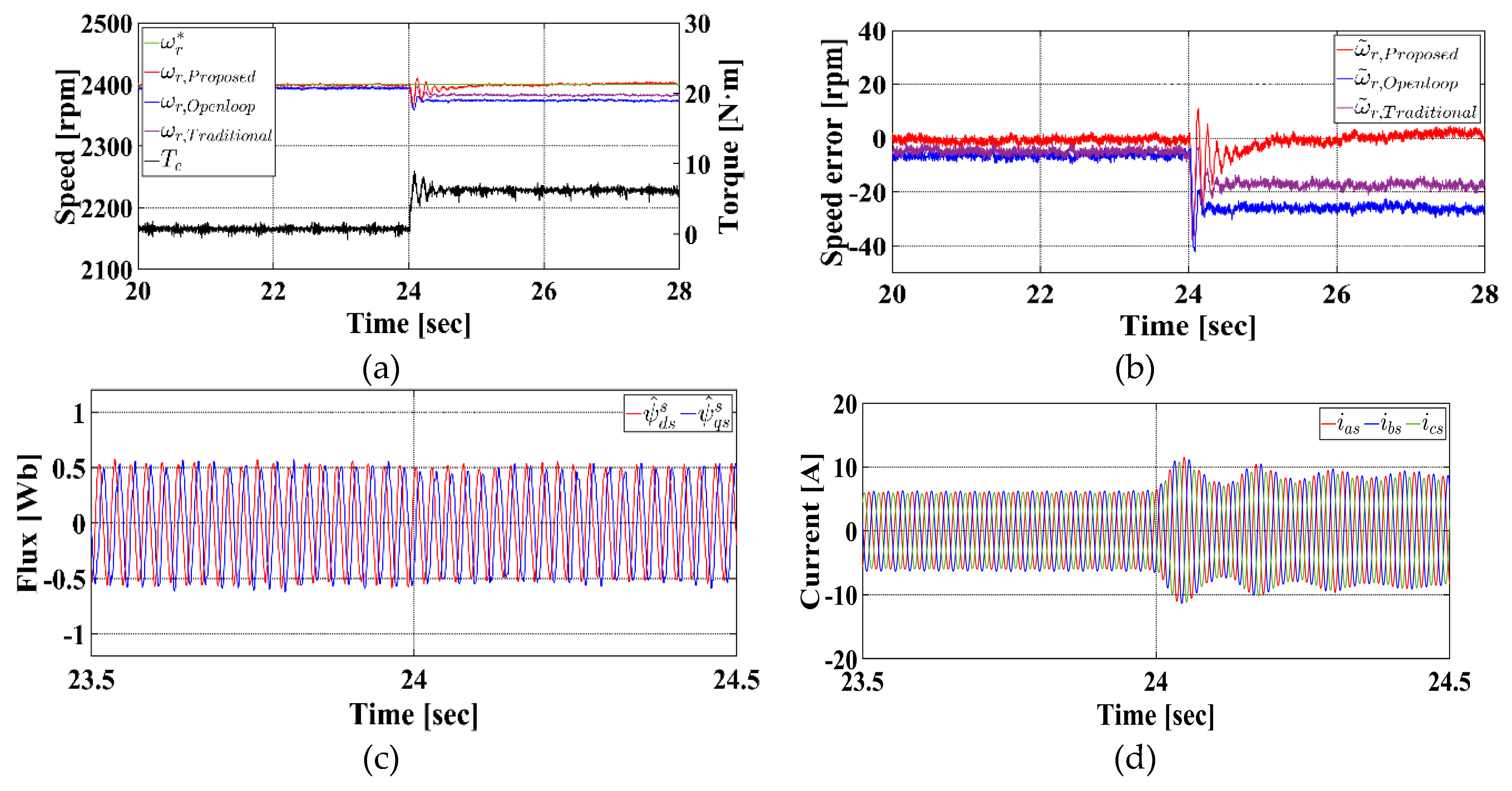
Figure 11.
Experiment result at 50 % rated load: (a) Overall, (b) Steady-state, (c) Estimated flux, and (d) Three-phase current.
Figure 11.
Experiment result at 50 % rated load: (a) Overall, (b) Steady-state, (c) Estimated flux, and (d) Three-phase current.
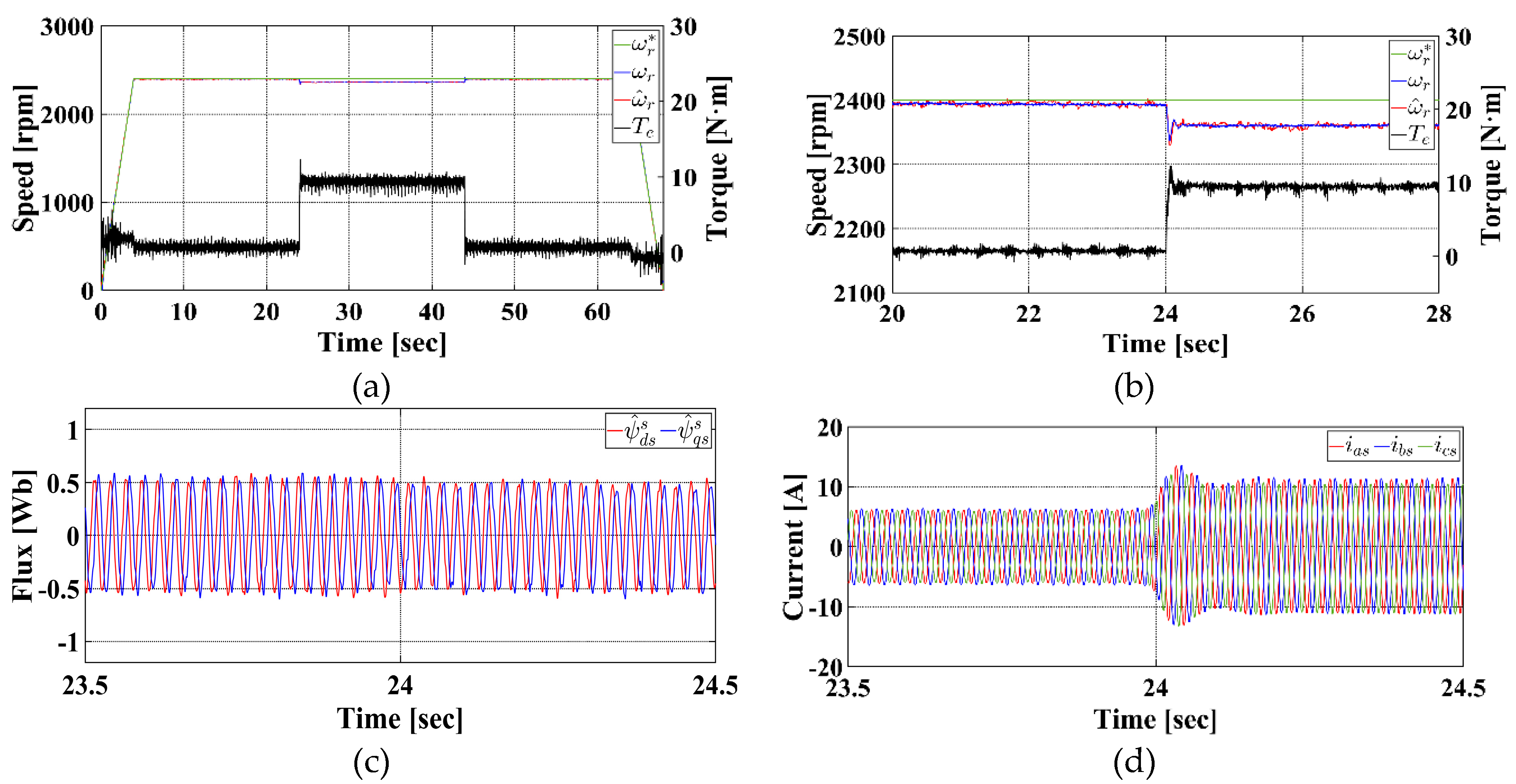
Figure 12.
Speed control result at 50 % rated load torque in experiment: (a) Speed comparison at steady state, (b) Speed error with reference speed, (c) Estimated flux, and (d) Three-phase current.
Figure 12.
Speed control result at 50 % rated load torque in experiment: (a) Speed comparison at steady state, (b) Speed error with reference speed, (c) Estimated flux, and (d) Three-phase current.
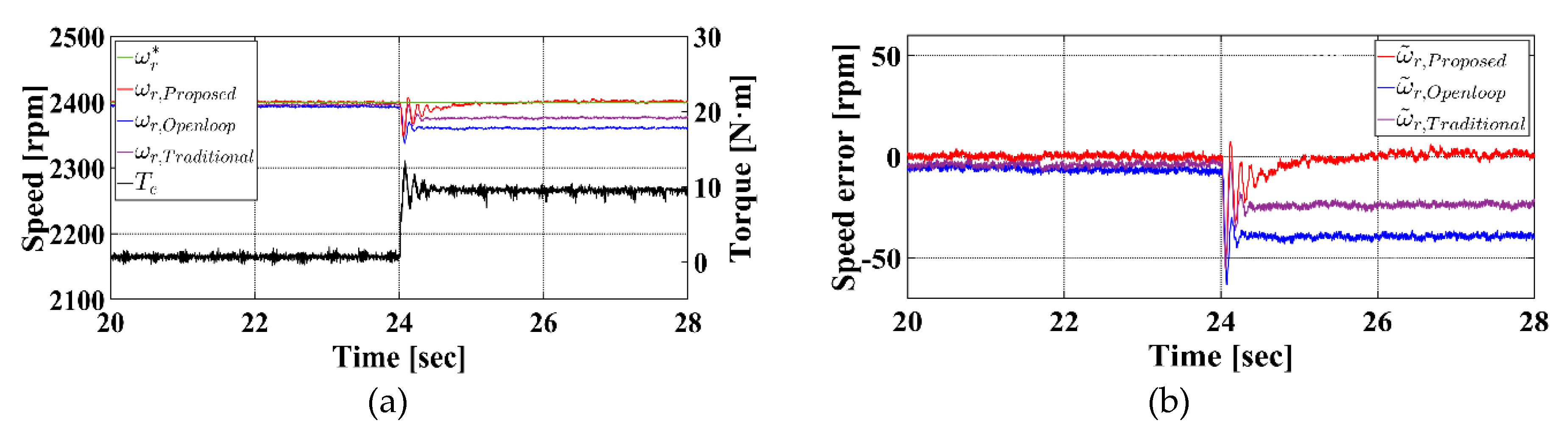
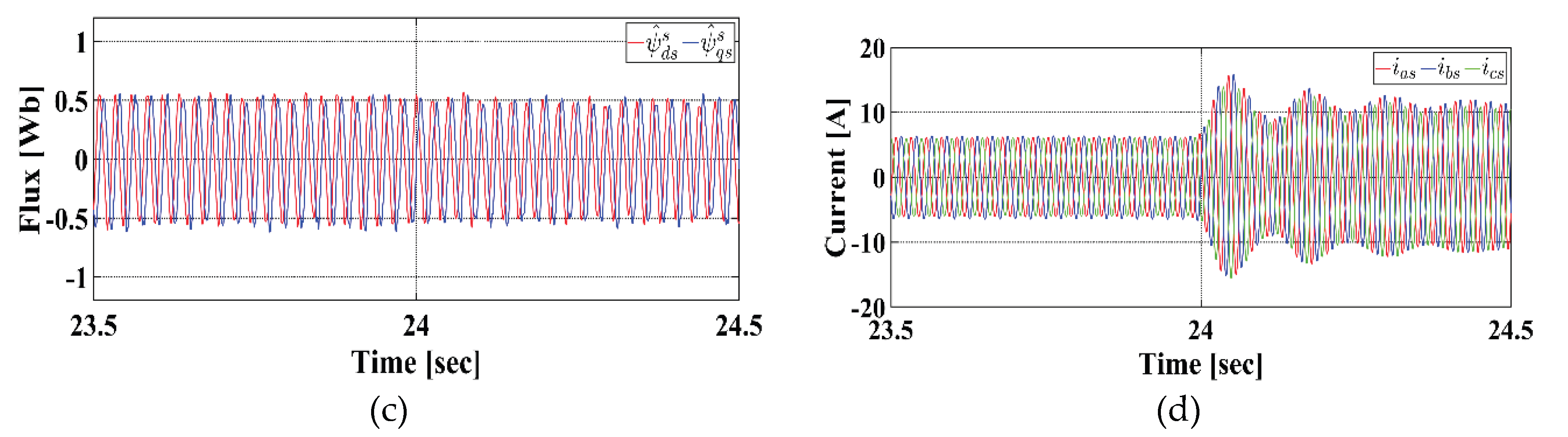

Table 1.
5.5 kW Induction Motor Parameters.
| Parameter | Value | Unit |
| Rated Output | 5.5 | kW |
| Rated Speed | 3,520 | rpm |
| Rated Torque | 14.91 | N∙m |
| Rated Voltage | 380 | V |
| Rated Current | 10.9 | A |
| Stator Resistance | 0.68 | Ω |
| Rotor Resistance | 0.49 | Ω |
| Stator Leakage Inductance | 3.4 | mH |
| Rotor Leakage Inductance | 3.4 | mH |
| Mutual Inductance | 0.13 | H |
| Inertia | 0.014 | kg∙m2 |
| Poles | 2 | - |
Table 2.
Speed control result comparison in simulation.
| Load Torque | Open-loop | Traditional | Proposed |
| 30 % (Error Rate) |
2,383.17 rpm (0.70 %) |
2,389.65 rpm (0.43 %) |
2,399.69 rpm (0.02 %) |
| 50 % (Error Rate) |
2,371.56 rpm (1.79 %) |
2,382.43 rpm (0.73 %) |
2,399.44 rpm (0.02 %) |
Table 3.
Speed control result comparison in experiment.
| Load Torque | Open-loop | Traditional | Proposed |
| 30 % (Error Rate) |
2,373.75 rpm (1.09 %) |
2,382.75 rpm (0.72 %) |
2,401.12 rpm (0.05 %) |
| 50 % (Error Rate) |
2,360.25 rpm (1.66 %) |
2,376.75 rpm (0.97 %) |
2,401.50 rpm (0.06 %) |
Disclaimer/Publisher’s Note: The statements, opinions and data contained in all publications are solely those of the individual author(s) and contributor(s) and not of MDPI and/or the editor(s). MDPI and/or the editor(s) disclaim responsibility for any injury to people or property resulting from any ideas, methods, instructions or products referred to in the content. |
© 2025 by the authors. Licensee MDPI, Basel, Switzerland. This article is an open access article distributed under the terms and conditions of the Creative Commons Attribution (CC BY) license (http://creativecommons.org/licenses/by/4.0/).
Copyright: This open access article is published under a Creative Commons CC BY 4.0 license, which permit the free download, distribution, and reuse, provided that the author and preprint are cited in any reuse.


