
Submitted:
14 July 2025
Posted:
16 July 2025
You are already at the latest version
Abstract
This paper proposes a learning-driven passivity-based control (PBC) strategy for sensorless induction motors, combining a nonlinear adaptive observer with recurrent neural networks (RNNs) to improve robustness and estimation accuracy under dynamic conditions. The main novelty is the integration of neural learning into the passivity framework, enabling real-time compensation for un-modeled dynamics and parameter uncertainties with only one gain adjustment across a broad speed range. Lyapunov-based analysis guarantees the global stability of the closed-loop system. Experiments on a 1.1 kW induction motor confirm the approach's effectiveness over conventional observer-based and fuzzy-enhanced methods. Under torque reversal and flux variation, the proposed controller achieves a torque mean absolute error (MAE) of 0.18 Nm and flux MAE of 0.21 Wb, compared to 1.58 Nm and 0.85 Wb with classical PBC. The peak torque deviation drops from 42.52% to 30.85% of nominal, torque symmetric mean absolute percentage error (SMAPE) improves by 7.6%, and settling time is reduced to 985 ms versus 1120 ms. These results validate the controller's precision, adaptability, and robustness in real-world sensorless motor control.
Keywords:
induction motor
; Lyapunov stability
; non-linear observer
; passivity control
; recurrent neural networks
; adaptive neural-fuzzy control
1. Introduction
The control of induction motors (IMs) continues to attract strong research interest due to their nonlinear structure, sensitivity to parameter variations, and widespread use in industrial applications. Traditional control methods often rely on accurate measurements of rotor speed and flux, which may not always be available or reliable in sensorless configurations. In this context, passivity-based control has emerged as a promising framework due to its solid theoretical foundation and robustness to system uncertainties. Early works demonstrated the use of passivity theory to ensure stable torque and flux regulation in IMs. For example, Cecati [1] proposed a passivity-based position controller, while Duarte-Mermoud [2] introduced an adaptive passivity approach for robust speed control. Travieso-Torres [3] extended this framework with adaptive structures for enhanced robustness under parameter variations. Moreover, Mansouri [4] applied passivity theory to sensorless IM control by integrating it with nonlinear observers for improved state reconstruction. In parallel, adaptive control strategies have played a pivotal role in addressing variations in machine parameters, such as rotor resistance and load torque, which frequently degrade control performance. Marino [5] introduced an adaptive input-output linearizing controller for IMs, achieving asymptotic tracking despite parametric uncertainties. Similarly, Chenafa [6] and Espinosa-Pérez [7] developed globally stable adaptive schemes using nonlinear feedback structures. In the sensorless domain, Belkacem Bekhiti [8], [9] proposed adaptive Luenberger and extended Kalman filter observers to enhance rotor speed estimation without mechanical sensors. More recently, Bekhiti [10] extended the adaptation ideas by validating a hyper-stability-based multivariable nonlinear adaptive control framework on induction motors, demonstrating strong experimental performance under non-ideal conditions. The integration of nonlinear state observers has further strengthened sensorless control by enabling full-state estimation based solely on measurable stator currents and voltages. Gauthier [11] and Busawon [12] contributed to the theoretical foundations of nonlinear observers, while Mansouri [13] tailored these concepts to IMs operating under field-oriented control. These observer designs significantly improve robustness and observability, especially at low speeds and under load disturbances.
More recently, artificial intelligence (AI) and neural networks have emerged as powerful tools in intelligent motor control. Neural models can approximate complex nonlinear mappings and adapt online, making them particularly suitable for estimation and control in dynamic environments. Beltran-Carbajal [14] and Moghadasian [15] proposed neural network-based controllers for IMs that adapt to system variations in real time. Sujatha and Vaisakh [16], along with Brandstetter and Kuchar [17], demonstrated the effectiveness of adaptive neuro-fuzzy inference systems (ANFIS) and radial basis function (RBF) networks in sensorless IM control. Acikgoz [18] implemented a real-time speed controller using a type-2 fuzzy neural network, while Hussain [19] introduced a type-II adaptive neuro-fuzzy controller with strong transient response capabilities.
Several studies have specifically integrated AI-based observers into MRAS or passivity-based frameworks. For instance, Medjadji [20] and Govindharaj [21] enhanced speed estimation using fuzzy and neuro-fuzzy observers. Parimalasundar [22] combined artificial neural networks with sliding mode control for power steering applications, and Mekrini [23] applied fuzzy logic in the control of asynchronous machines. Recent contributions by Sun [24] and Mienye [25] explored adaptive learning and recurrent neural network architectures to further strengthen robustness. Wu [26] addressed neural optimization by improving the convergence of online learning through gradient normalization—relevant for real-time motor drive applications.
Despite significant progress in adaptive, passivity-based, and learning-driven control of induction motors, a critical gap remains in unifying these approaches into a robust and practical sensorless control framework. Existing methods often treat passivity and learning separately or rely on fixed observers with limited adaptability. Neural and neuro-fuzzy controllers, while effective in handling nonlinearities, frequently lack formal stability guarantees or disrupt the energy-preserving structure of the system. These limitations become especially pronounced under low-speed operation, load transients, and parameter variations, which are common in industrial applications. Moreover, many nonlinear observers are structurally complex or computationally intensive, making real-time implementation difficult. This motivates the need for a cohesive control architecture that integrates the stability of passivity theory, the adaptability of neural learning, and the practical efficiency of nonlinear observer design in a fully sensorless setting.
This paper addresses the above challenges and presents a unified learning-driven passivity control strategy for induction motors using a nonlinear neural-adaptive observer. The main contributions are summarized as follows:
- A novel neural-based adaptive observer is proposed to estimate rotor flux and speed in real time, enhancing estimation accuracy under partial observability and eliminating the need for mechanical sensors.
- A nonlinear passivity-based control law is developed that integrates the neural learning loop while preserving passivity and ensuring global asymptotic stability.
- Experimental validation is conducted on a 1.1 kW induction motor under dynamic benchmarks (speed reversal, torque steps, and parameter variations), demonstrating up to 88.6% reduction in torque error and 75.3% improvement in flux estimation accuracy compared to classical methods.
This architecture bridges the gap between model-based passivity control and data-driven adaptation, offering a scalable and robust solution for high-performance industrial IM drives. The remainder of this paper is organized as follows: Section 2 presents the nonlinear dynamic model of the IM motor and the passivity framework. Section 3 details the neural adaptive observer design and learning algorithm. Section 4 introduces the passivity-based control strategy and its integration with the observer. Section 5 describes the experimental platform and test scenarios. Section 6 presents and discusses the results. Finally, Section 7 concludes the paper and outlines future directions.
2. Mathematical Framework and Problem Statement
Before deriving the control laws, it is essential to establish a physically consistent mathematical model of the induction motor that captures the key electromechanical dynamics relevant for observer and controller design. The modeling approach adopted here is based on an energy-based formulation that reflects the internal coupling between electrical and mechanical subsystems. This framework serves as the foundation for the passivity-based and adaptive structures developed later in the paper.
2.1. Dynamic Model of an Asynchronous Motor
In the mathematical analyses, it is standard practice to substitute the squirrel-cage motor, (rotor is characterized by uniform distributed conductors), with a theoretical equivalent rotor. This theoretical model matches the stator in the number of phases and features conductors distributed in a sinusoidal pattern. This method operates under the assumption that only the fundamental harmonic of the rotor’s magnetomotive force (MMF) is considered. Practical findings confirm that analyses and controller designs using this reduced model are applicable to the actual machine. However, special attention is required when modeling wound rotors using sinusoidally distributed windings [27,29]. The dynamic model is derived through the direct use of Euler-Lagrange formalism, as outlined in [10] which results to (differential Lagrangian system):
Or more compactely we write:
The conventional two-phase αβ model, where the stator axes are stationary and the rotor axes rotate at the electrical angular velocity, is commonly used for a p pole-pair squirrel-cage induction motor with a uniform air-gap. This model defines the electrical parameters that are essential for analysis and control design.
The current vector is: with, , , . The flux vector is related to the current vector via . To carry out the controller design, a suitable linear factorization of these workless forces into a form
In particular, the matrix must be chosen such that is skew-symmetric, and its 3rd-4th rows are independent of the quantity. These conditions are necessary for the subsequent stability analysis. By utilizing the transpose of and, it becomes apparent that the desired objectives can be attained with the following selection
This decomposition results in the next compact model [13]:
with ,, , , and
2.2. Problem Formulation
Consider the induction motor model given by Eq(6) with outputs and to be controlled. Assume that:
A1 is an unknown constant (switched step).
A2 are accessible.
A3 All parameters are well-known and .
Let be a differentiable function, with a known bounded, first-order derivative, and let β(t)>0 be the desired norm of the rotor flux, which is a twice differentiable with known, bounded 1st and 2nd-order derivatives. Under these assumptions, the goal is to design a nonlinear control law that guarantees the stability (i.e. internally) and the asymptotic tracking of both and β(t). This control law must guarantee that, for any initial conditions, all signals within the closed-loop system remain uniformly bounded, thereby achieving the desired system performance.
To address the need for accurate flux and torque estimation using only stator-side measurements, we proceed to design a reduced-order nonlinear observer formulated in the stationary αβ reference frame. The observer is structured to be consistent with the motor’s energy-based dynamics and is later augmented with a recurrent neural network to enhance estimation accuracy under nonlinearities and uncertainties.
3. Nonlinear Observer Design
In this section, we review several flux observer designs from the literature, followed by the development of a tailored observer formulated specifically for the nonlinear framework considered in this work.
3.1. Flux Observer in a Closed Loop
A foundational reference in this area is the observer introduced by Verghese and Sanders [32], which has since inspired several variants, including those proposed by De Luca and Ulivi [33], Garcia in [34], and by Mansouri [4]. The general structure of this classical observer is given by:
where , , , , , the being scalars and . Note that the gains depend on the speed in (8). We show the diagram block of this observer in Figure 1.
The resulting model for the observer error dynamics is then
Note that we can freely determine the scalar coefficients in equation (9). If and are selected such that , the error dynamics become
We select and to place the eigenvalues of in arbitrary positions. Note that the characteristic polynomial of is . If the eigenvalues of are (twice) and (twice), then the eigenvalues of time varying matrix are and using the slow dynamics theory.
3.2. The Proposed Nonlinear Intelligent Observer Design
Passivity-based control strategies are widely recognized for their reliance on rotor flux information, which is often challenging to measure directly. Consequently, considerable research efforts have been directed toward developing methods for estimating these values. Now, we introduce the design of a reduced-order flux observer for an asynchronous motor operating in the αβ reference frame. The proposed observer requires inputting only the stator voltage, current, and rotor speed. Specifically, this new nonlinear-observer incorporates the speed measurements, ensuring that only the electrical quantities are required in the estimation process [13]. Consider the αβ model for induction motor:
where
The system (11) is the form
with
Here, we make the following assumptions as posed by K. Busawon (see [12])
(A4) There exists a class of bounded admissible controls, a compact set and positive constants α, β > 0 such that for every and every output associated with and with an initial state , we have .
(A5) and its time derivative are bounded.
(A6) The matrix is of class , with respect to their arguments.
(A7) Functions , are global Lipschitz with respect to uniformly in and .
We characterize the observer design for the system (12) in the following theorem
THEOREM: 1 Assume that the system (12) satisfies Assumptions (A4) to (A7). Then there exists such that the system
is an exponential observer for the system (12), where is the unique solution of the algebraic Lyapunov equation , , , and the explicit formula of is
Moreover, we can make the dynamics of this observer arbitrarily fast. ∎
So, by multiplying the left and right-hand sides of (14) by and respectively, the following algebraic equation holds:
The choice of θ permits the pole placement of the observer according to the speed.
In summary the system can be written as or
The observer is or
So the error equation is with or
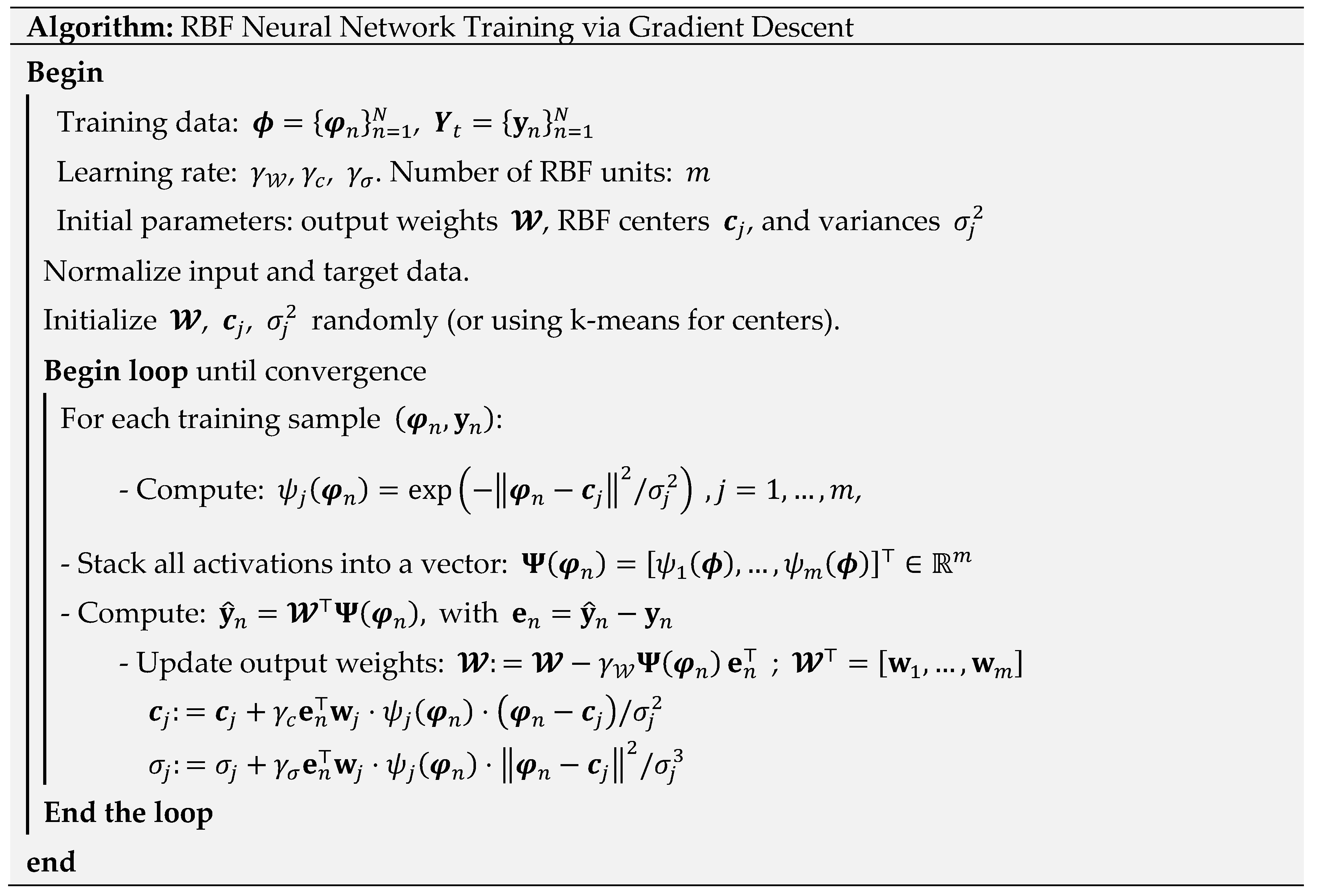
To incorporate learning-based compensation for model uncertainties and to enhance the robustness of the nonlinear observer, we introduce a radial basis function neural networks (RBFNN) term into the observer dynamics. The network approximates unknown disturbances or residual nonlinearities using a regressor composed of observable and estimated signals. Let represent an unknown nonlinear function (e.g., modeling error or disturbance). The universal approximation theorem states that, for any continuous function , there exists a feedforward neural network (three-layer NN) of the form: with or we omit the intermediary variable as where
- is the activation vector,
- is the output weight matrix,
- are nonlinear sigmoids activation functions (e.g., tanh, ReLUs, etc.).
- : stacked weight matrix ( row is ), : stacked biases,
- The exponential and division are element-wise.
The coefficients and are the hidden layer parameters ( Input-to-hidden weights "nonlinear layer" and are the Bias of neuron ). Now, the resulting enhanced observer is given by:
Here, is the adaptive weight matrix of the neural network and the vector is a vector of radial basis activation functions, typically Gaussian ( and is the regressor vector, e.g., ). The network parameters are updated online via adaptation rules derived from Lyapunov stability analysis to ensure convergence and passivity preservation. The RBF neural term is added as a correction to the standard observer dynamics, to compensate for unknown nonlinearities or disturbances not captured by and . This term acts like a learning system and is updated online (see Figure 2).
So the RBFNN becomes: . In order to train the RBFNN we should to minimize the squared error objective function: . To adapt , perform . Again, for we have: . Here is a formal description of this training algorithm
3.3. The Proposed Fuzzy-MRAS Estimator
Rotor speed can be estimated using a model reference adaptive system (MRAS) structure composed of two estimators: a reference model and an adaptive model. Both models independently compute the rotor flux linkage components and in the stationary αβ reference frame. By comparing the flux-linkage estimates, the adaptive model adjusts its internal speed estimate to minimize the discrepancy, thereby converging to the true rotor speed [8,9]. The reference model, derived from the stator voltage equations, does not depend on rotor speed and is therefore suitable for speed-independent flux estimation. Its expression in the stationary frame is given by:
In contrast, the adaptive model, formulated from the rotor voltage equations, explicitly depends on the rotor flux components and the estimated speed . It is expressed as:
The angular discrepancy between the estimated and reference flux vectors serves as the adaptation signal, which is processed by a linear PI controller to adjust the estimated speed. Applying the Popov criterion [10,20] to guarantee global asymptotic stability of the closed-loop estimation system, the adaptive law is given by:
Fuzzy logic is particularly advantageous for systems that are difficult to model analytically, due to limited data availability, incomplete information, or the inherent complexity of the underlying process [16]. These systems can be easily extended by adding new rules, allowing for performance enhancements and the inclusion of additional features. In conventional MRAS-based speed observers, a proportional-integral (PI) controller is typically employed within the adaptation mechanism to estimate rotor speed by minimizing the error between the reference and adaptive models [18]. In the proposed approach, the PI controller is replaced by a fuzzy logic controller, as depicted in Figure 3. The complete block diagram of the fuzzy controller is presented in Figure 4, and its internal structure is illustrated in Figure 5. The fuzzy logic system operates by first processing the input variables through a fuzzification stage, where crisp input values are mapped to fuzzy sets using predefined membership functions and scale transformations. This scale mapping adjusts the range of the input variables to match the domain expected by the controller. The rule base stores the fuzzy inference rules, while the inference mechanism applies these rules to derive fuzzy conclusions. Common inference strategies include the Mamdani method, which typically uses the logical AND operator for rule evaluation, and the Takagi-Sugeno Model (TSM), which generates functional outputs based on the input variables [23,36]. Finally, the defuzzification stage converts the fuzzy output set into a crisp control signal suitable for direct application to the system.
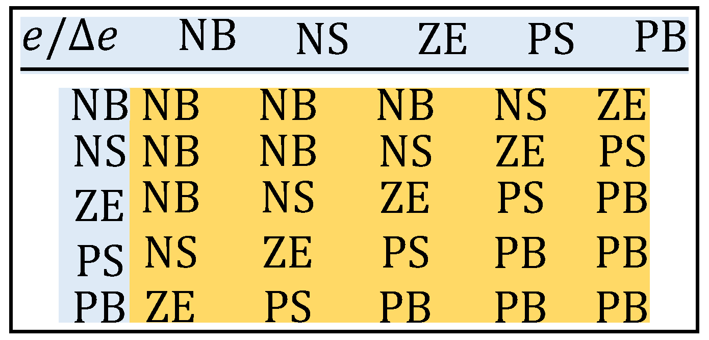
Knowing that gains , and are scaling factors, they should be chosen carefully after doing trial and error technique to get the optimal performance of the controller. From the expert estimator, the following memberships of fuzzy sets are used. The rules supporting this system are expressed in the Table 1, where NB: Negative Big, PB: Positive Big, NS: Negative Small, PS: Positive Small and ZE: Zero Equal. The number of inputs to the fuzzy controller can be 2 or 3. In the proposed method to reduce the complexity the two inputs are considered. The linguistics values that can be considered for each input are 3, 5, 7 or 9 as the case may be. Since there are two inputs, the numbers of rules that are possible are or which gives 9, 25, 49 or 81 rules for the above linguistic values respectively. The choice of linguistic value should be made keeping into consideration that the control should be good and computation taken by the fuzzy controller should not be high make the process slow. The linguistic value 3 which gives 9 rules is too small to get the better control. Figure 6 shows the fuzzy membership functions and control surface of the proposed adaptive system.
, change in and the control surface of the fuzzy logic estimator
The fuzzy inference rules used in the proposed system are summarized in Table 1.
4. Passivity Based Output-Feedback Controller
4.1. Non-Intelligent Sensorless Adaptive Passivity-Based Controller Design
The fundamental concept of passivity lies in shaping the total energy of the system and introducing an additional damping term to guide its dynamic behavior. Using the Euler–Lagrange modeling (ELM) framework, the total energy expression can be systematically formulated and then shaped toward a desired minimum. If the control input is designed to inject a supplementary dissipative term into the system, the convergence to the equilibrium state can be significantly improved beyond what is achieved through the system’s natural dissipation alone. In essence, passivity is an intrinsic property of certain physical systems and is closely linked to the notion of input–output stability [10,35].
: , called a storage function, with , as for all , and , it is satisfied
where is a continuous storage function with continuous derivatives of order . Condition (20) can also be expressed as [29]. The system is said to be lossless when . ∎
In cases where the nature of the system does not involve any motion of coordinates or changes in reference frames (systems that are not explicitly time dependent), the Hamiltonian is simply the total energy of the system. The Hamiltonian of IM (i.e. conservative system with zero potential energy) equals the sum of the kinetic energy and the potential energy
The time derivative of this Hamiltonian function along the trajectories of the system can be expressed as
Using the previous equations and we get
So, the derivative of Hamiltonian function of IM is given by:
Because we deduce that
This outcome proves that the system (IM) is passive, hence the of the induction motor is proved. Also we note that the vector given by contains the forces which do not produce work. As the IM system is an interconnection of two subsystems (electrical and mechanical see Figure 7) then it can be shown that each of the two subsystems are passive; so we arrive at a new approach to the structure of passivity based on the fact that the interconnection of two passive subsystems is passive.
We consider the total energy of the electrical subsystem: , then the time derivative of this along the trajectories of the electrical system can be expressed as
So, the derivative of this Hamiltonian function is given by by integrating this, we obtain
Because we deduce that
This inequality gives us:
which proves the passivity of the electrical subsystem. On the other hand the mechanical subsystem is positive real for all and which is also passive.
PROPOSITION: 1 Consider the asynchronous motor given by equation(6) with outputs and to be controlled, and assumptions A1 to A3. Let the control law be defined as,
The superscript is the desired variable, with
and with the following controller dynamics and .
The gains and are given as
with . while the state estimator and the load adaptation law are
where , and
Under these conditions, the closed-loop system guarantees global tracking of torque and flux norm, while ensuring all signals remain uniformly bounded. ∎
Proof:
Because the control law utilizes the estimated states rather than the actual ones, as opposed to the ideal scenario, the error dynamics in this case are:
where , and
Alternatively, based on equations (34) and (1), the observation error satisfies the following equation: . So, consider the following Lyapunov function candidate
Knowing that is skew-symmetric and which yields the derivative
Use of equation (35) in the equation above and let we define, which results in the next quadratic function with
Verifying that guarantee the strict positive definiteness of, i.e. ∎
To enable full sensorless operation prior to incorporating intelligent learning, the control framework is first augmented with a conventional PI-based speed estimator. This allows rotor speed reconstruction from electrical measurements alone, eliminating the need for mechanical sensors while preserving the structure and stability of the original passivity-based control loop.
The estimation flux is used to drive a PI-like update law for . A standard structure is:
is the error between the real and estimated rotor fluxes and currents.
The overall architecture of the non-intelligent sensorless adaptive passivity-based controller is illustrated in Figure 8.
Although the previous controller ensures tracking and robustness via passivity control, its performance may degrade under unmodeled dynamics or uncertainties. To enhance adaptability, a recurrent neural network is integrated to learn residual dynamics in real time, yielding an intelligent adaptive control.
4.2. The Proposed Intelligent Adaptive Passivityt Based Controller Design
The proposed intelligent adaptive passivity-based controller integrates neural learning for enhanced sensorless performance. As shown in Figure 9, a recurrent neural network estimates both the load torque and rotor speed , enabling full sensorless operation. These estimates drive a passivity-based control loop to generate stator voltage commands, ensuring robustness in both steady-state and dynamic conditions.
The proposed scheme employs a recurrent neural network to estimate the load torque and the rotor speed . By capturing temporal dependencies, the RNN effectively models the motor’s nonlinear dynamics, outperforming conventional feedforward networks. Let and denote the speed and the electromagnetic torque errors, at discrete time step . The internal structure of the RNN is governed by the following equations [25,26]:
- 1.
-
Hidden State Update: where:
- : hidden state vector, : bias vector,
- : input weight matrix, : recurrent weight matrix,
- : element-wise activation function (e.g., tanh or ReLU).
- 2.
-
The Output Estimation: where:
- : output weight vector, : output bias.
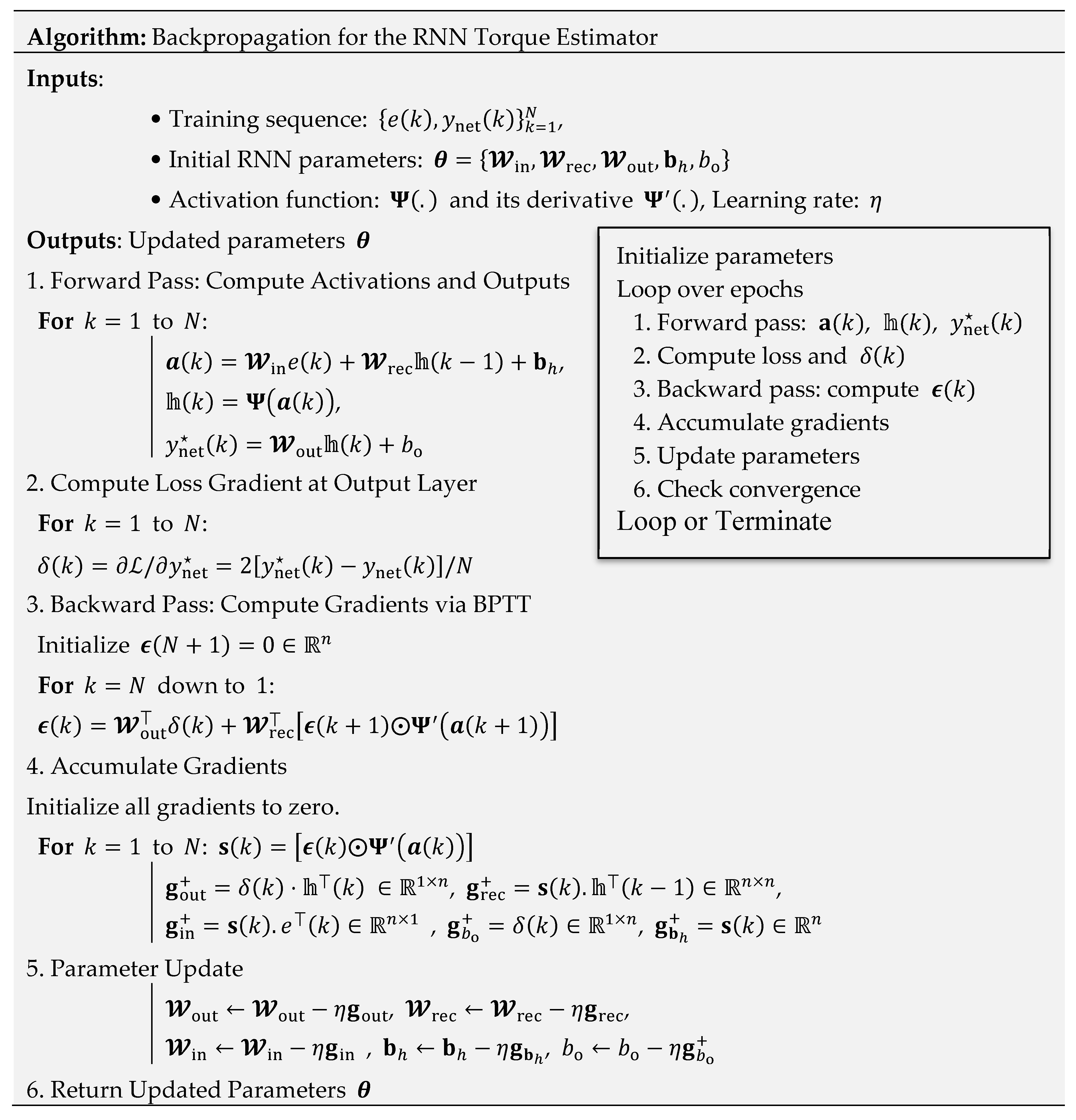
The complete mapping from input error to the nedded estimate is compactly expressed as one function: where is the set of all trainable parameters [30]. This RNN-based estimator enables the controller to adaptively generate commands that account for the system's nonlinearities, time delays, and dynamic uncertainties, thus enhancing overall control performance. The RNN parameters are optimized to minimize the mean squared error loss: . First we compute hidden states and output estimates sequentially: and then compute gradients by unrolling the network through time and applying the chain rule. Finally, update parameters using gradient descent or an advanced optimizer (e.g., Adam): where is the learning rate. This iterative process continues until convergence, enabling the RNN to learn the dynamic mapping from error sequences to the output commands effectively [31]. If we define then the gradients for output layer are given by and . Also, if we back-propagate through time (BPTT) into hidden states then we compute recursively (i.e. ) as where , is the element-wise derivative of activation function and is the element-wise multiplication. Now use to compute the following gradients: , and with . Finally, if we let be the learning rate, then we can updtae: , etc. All parameters are updated this way. The structure of this learning procedure is given in the flowchart shown in Figure 10
The RNN parameter update steps using BPTT are described in the following algorithm
5. Experimental Results and Discussion
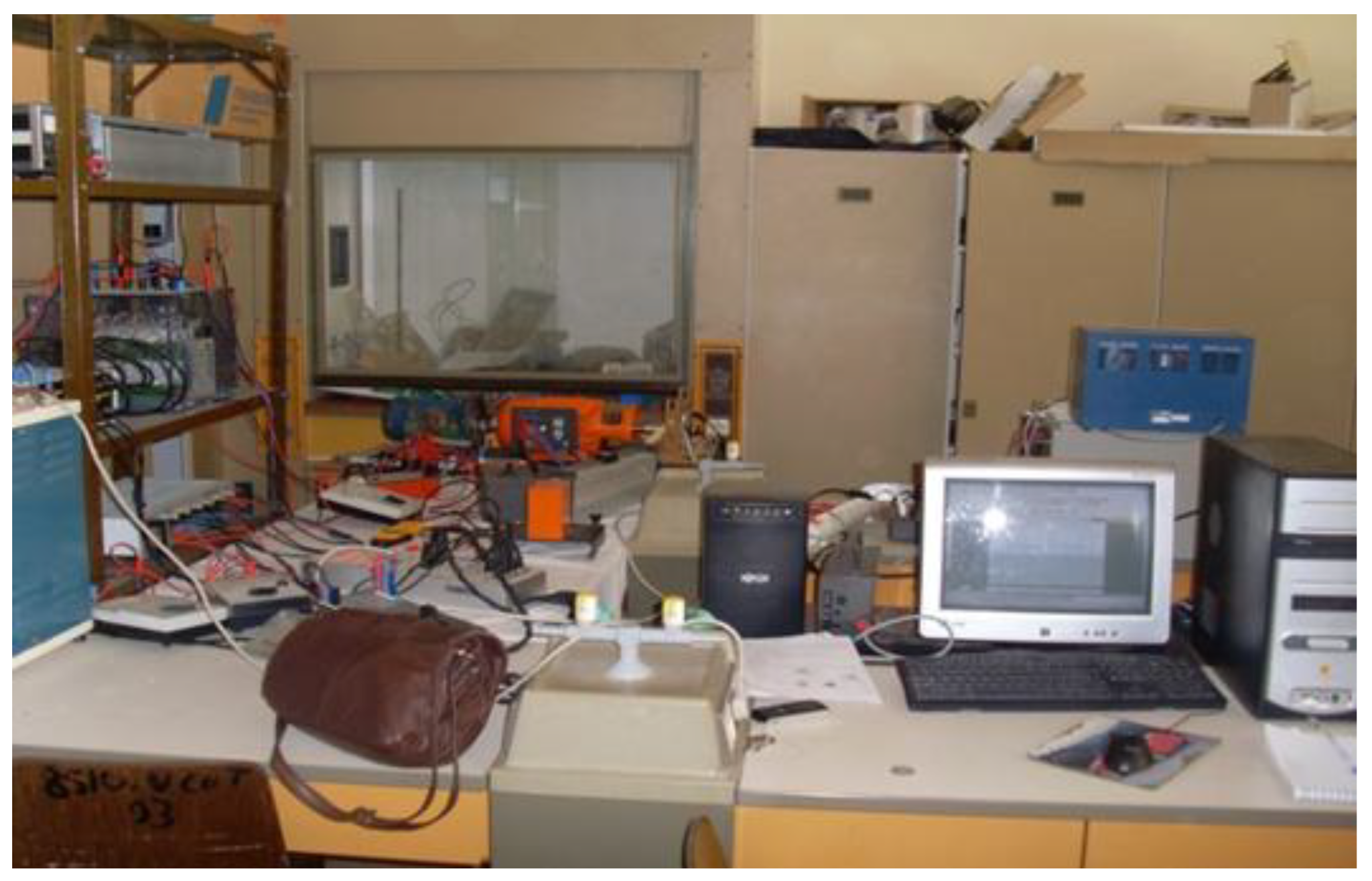
The neural passive controller has been tested on a test setup (Figure 11) which consists of:
- Three-phase induction motor with rated values:
• Synchronous machine with powder brakefor for loading the IM.
• Electronic power converter (without any control system):
• 3 (three-phase) diode rectifier and
• VSI composed of three IGBT modules
• Electronic card for monitoring the stator phase with
• Instantaneous voltage sensors (LEM LV 25-P) and
• Instantaneous current sensors (LEM LA 55-P)
• Voltage sensor for monitoring the instantaneous value of
• The dc-link voltage. (model LEM CV3-1000)
• Incremental encoder only for comparison measurements.
• Model RS 256-499, 2500 pulses per round, (for validation-comparison, not for control)
• card () with a PowerPC at and floating-point digital signal processor . During the real-time operation of the control, the supervision/capturing of the important data can be done by the software provided with board.
Figure 11.
Experimental setup for the proposed neural-PBC daptive control of the IM.
Simulations in MATLAB verified the proposed control scheme using a rated flux reference and DC-link voltage. The feedback signal reconstruction was confirmed in simulation, and experimental results further validated the effectiveness-robustness of the sensorless control strategy. The electrical and mechanical parameters of the induction motor are listed in Table 2.
The “Control/Command” part is based on the R&D Controller Board developed by the German company dSPACE and housed in a computer. This control card is made up of two processors. The master processor manages the application while the slave processor, a DSP (“Digital Signal Processor”) from TEXAS INSTRUMENT (type ), generates the (Pulse Width Modulation) control signals in 0/5 V TTL logic. This constitutes the “hardware” part of .. The "software" part consists of two software programs. The first, , allows easy programming of the real-time application under Simulink by using specific blocks (Belonging to the "Real Time Interface () toolbox") allowing the configuration of the inputs/outputs of the card. The second software, , allows the program code to be loaded onto the card (written in graphical form in Simulink, compiled and transformed into C code), to create a complete experimental environment and in particular a graphical interface for controlling the real-time process, to process the data and save it in a format compatible with (for later processing) or even to monitor in real time the evolution of the measured or calculated data using graphical or digital displays. The exchange of information between the two parts described is carried out via an external connection box (Connector Panel from ) connected to the card via a shielded cable and receiving the analog signals via connectors, an interface for conditioning the control signals and any error signals returned by the Semikron converter and a measurement environment consisting of various sensors. The signal conditioning interface converts the signals from 0/5 V logic to 0/15 V logic and vice versa. This modification is essential because the control card works with 0/5 V logic signals, while these must be in 0/15 V logic for the voltage inverter. The measurement environment consists of LEM type LA25TP sensors (closed-loop current sensors using the Hall effect) for current measurements, LEM type LV100-500 sensors (closed-loop voltage sensors using the Hall effect) for voltage measurements and an incremental encoder to measure the motor rotation speed. Finally, the measured analog currents are intended for digital processing and must therefore be sampled. Therefore, in order to avoid any spectral aliasing phenomenon, it is necessary to insert a guard filter (with an estimated cut-off frequency of 500 Hz, one order of magnitude above the fundamental frequency of 50 Hz) between each sensor and the analog-to-digital converter.
Analyzing the operation of an IM supplied by a voltage inverter is complex due to its complicated nonlinear nature. Moreover, neural (or neuro-fuzzy) adaptive control of an IM requires solid theoretical foundations in areas such as electrical machines, power electronics, and control systems. Using the -instrumented platform, the proposed control strategy is first implemented in Simulink, then deployed in real-time via . The -driven inverter operates at a switching frequency of . A detailed view of the experimental setup is provided in Figure 12.
5.1. Study of the Proposed Nonlinear Intelligent Observer
The performance of the proposed nonlinear observer is first evaluated in open-loop and then integrated into a closed-loop configuration with the nonlinear controller of the induction motor. To align the observer dynamics with those of the plant, a tuning parameter is used. The trajectories of the motor and observer poles, are experimentally analyzed under this setting. Figure 13 illustrates the rotor flux observation error obtained at various operating speeds (0.0125, 3.4, and 150 rad/s), with , demonstrating the accuracy and robustness of the observer. The given architecture is tested under different perturbation scenarios, including parameter variations and unmodeled dynamics, to validate the strength and reliability of the proposed intelligent strategy.
The convergence characteristics of the proposed nonlinear observer are significantly affected by the tuning parameter , which shapes the placement of its eigenvalues relative to those of the motor. As shown in the upper subplots of Figure 14, increasing shifts the observer poles (blue) to follow the motor poles (red) more closely across the operating range to 400 rad/s. For , the observer exhibits a moderately damped response, while yields faster convergence with reduced transients. The lower subplots of Figure 14 illustrate the corresponding rotor flux observation errors under three representative speeds (0.0125, 3.4, and 150 rad/s). In both cases, the observer demonstrates strong convergence properties, but higher improves transient rejection and tracking precision, especially at low and nominal speeds.
To evaluate the sensitivity of the proposed nonlinear observer to rotor resistance variations, Figure 14 presents experimental results under three resistance values: (nominal), (+50%), and (+100%). The observer is initialized with rotor flux components set to .
Figure 14 demonstrates that, even with increased from (nominal) to (+50%) and (+100%), the nonlinear observer ensures rapid flux convergence. At both nominal (150 rad/s) and low speed (60 rad/s), transients settle within 0.6 s, showing strong disturbance rejection. A small steady-state offset remains (about 0.15 Wb at +50% and 0.30 Wb at +100%) indicating sensitivity to parameter mismatch. To address this, an RBFNN-based observer is introduced (Figure 14), incorporating an adaptive term that continuously compensates for rotor resistance errors and effectively eliminates steady-state flux bias under large uncertainties.
Figure 15 highlights the impact of the RBFNN augmentation on the observer’s transient performance under large rotor resistance variations. In the baseline observer, the flux error exhibits pronounced oscillations and peak deviations nearing 0.8 Wb for a +100 % resistance change, with settling oscillations persisting beyond 0.6s. With the RBFNN-enhanced observer, the peak error is reduced by over 50 %, and oscillations are significantly damped—settling in under 0.4 s across all resistance cases. This clear reduction in transient amplitude and faster damping confirms that the online neural adaptation effectively compensates for parameter mismatches, yielding smoother and more responsive flux estimation throughout the speed range.
Mismatch.
5.2. Comprehensive Evaluation of the Proposed Nonlinear Intelligent Passivity-Based Control
This section presents an overall assessment of the proposed nonlinear intelligent passivity-based control, which integrates a neural PBC controller, an RNN-based adaptive observer, and a sensorless speed estimator. The complete system is tested in closed-loop with the induction motor under various conditions, including load disturbances, speed reversals, and parameter variations. The results highlight the dynamic performance of key signals such as torque, rotor flux, speed, and control voltages, confirming the robustness, adaptability, and precision of the proposed scheme. Figure 16 presents these responses under all test scenarios.
The performance of the proposed nonlinear intelligent PBC strategy is illustrated in Figure 16, which presents both control and estimation results under time-varying speed and load torque conditions. The top-left subplot shows that the controlled electromagnetic torque tracks the reference smoothly with minimal steady-state error. The top-right plot confirms accurate load torque estimation , closely matching the timing and magnitude of applied disturbances. The middle-left subplot shows that both estimated and measured speeds follow the commanded reference throughout acceleration, cruising, deceleration, and re-acceleration phases. The speed error, shown bottom-left, remains within ±8 rad/s, demonstrating the precision of the RNN-based speed estimator. The control voltages and , in the middle-right plot, reach ±250 V with consistent modulation behavior. The bottom-right plot shows torque error bounded within ±0.5 Nm, confirming high tracking accuracy and effective disturbance rejection. These results validate the proposed architecture’s capability for precise tracking, reliable estimation, and smooth control under sensorless operation.
Figure 17 was performed on a sensorless induction motor using the proposed PBC strategy for torque and flux control. The system faced load variations, noise, and rotor resistance mismatch, with all estimations handled observer-based. Control ran in real time with PWM injection, and key signals were precisely recorded for evaluation. The applied torque includes direction reversals to assess robustness.
The experimental results clearly confirm the effectiveness of the proposed nonlinear intelligent passivity-based control strategy. The motor tracks the torque reference with high accuracy, including during rapid transients and full torque reversal, maintaining a peak error within ±0.2 Nm. The estimated load torque closely matches the real applied load, capturing both magnitude and timing under dynamic conditions. The speed response aligns well with the reference, and the speed estimation remains precise even during acceleration and sharp changes. The flux estimation error is well confined within ±0.1 Wb, indicating strong observer performance. Input voltages exhibit clean modulation without saturation or chattering, demonstrating the quality of PWM-based voltage control. Despite load disturbances, parameter uncertainties, and full sensorless operation, the controller preserves stability, accurate tracking, and robustness, confirming its suitability for advanced industrial applications.
5.3. Comparative Study and Performance Evaluation
To evaluate the performance of the proposed control, we use standard electrical engineering (EE) control metrics based on the response to torque amplitude or flux amplitude (i.e. |final − initial|):
• is the time at which the response signal has covered 2% of the ramp amplitude.
• is the time after which the response remains at less than 5% of the target value.
• Peak overshoot relative to target (% of ramp amplitude).
• (steady-state error settling) the error once the has been reached.
• Error when reference reaches 50% of ramp.
• Max torque deviation during speed ramp.
And in order analyze the performance at global scope, we employ standard machine learning (ML) metrics: mean absolute error (MAE), symmetric mean absolute percentage error (SMAPE), and coefficient of determination (). These metrics are defined as: ; and where is the ground truth, is the predicted output of the model at time , and is the total experiment duration. denotes the mean of . These metrics jointly characterize accuracy, relative error, and explained variance, enabling a comprehensive assessment of model fidelity.
To comprehensively assess the effectiveness of the proposed adaptive neuro-PBC sensorless control scheme under realistic and demanding operating conditions, two benchmark trajectories were designed:
- Pseudo-Static Benchmark: The torque reference ramps from 0 to 8 Nm in the first second and remains constant for the rest of the experiment. During the period from 1 s to 3 s and 5 s to 8.5 s, a flux reference step of 8 Wb is applied with superimposed ripples to emulate disturbances. This test evaluates steady-state tracking and disturbance rejection.
- Dynamic Benchmark: Here, the torque follows a complex trajectory: it ramps from 0 to 8 Nm in the first second, holds steady until 5 s, then reverses sharply to approximately –8 Nm, followed by a final ramp back to 6 Nm by 10 s. Simultaneously, the flux reference features a sequence of four step changes (switch on to 8 Wb in some time intervals), testing the controller’s performance under rapid transients and flux variations.
Throughout the entire profile, small random perturbations are superimposed to simulate external disturbances, ensuring a challenging scenario for evaluating control robustness, responsiveness, and adaptation under dynamic and load-varying conditions. Figure 18 shows the profiles used during the experimental tests.
Now we present a comparative evaluation of the proposed neural adaptive PBC controller against four advanced control strategies. These include:
• CNO-PBC: classical PBC controll with a nonlinear observer,
• CFE-PBC: classical PBC controll with a fuzzy enhanced MRAS estimator
• CRBF-PBC: classical PBC controll with a RBF network enhanced observer, and a
• DRNN-PBC: deep learning adaptive PBC strategy with RNN network observer.
To evaluate steady-state accuracy and low-dynamic performance, all four control strategies were tested under the pseudo-static benchmark, where the torque reference ramps from 0 to 8 Nm within the first second and is then held constant. During the intervals and , a flux reference step of 8 Wb is applied, with superimposed ripple signals to emulate realistic disturbance conditions. This scenario is designed to assess tracking precision, overshoot suppression, robustness to steady-state perturbations, and the quality of torque/flux estimation in a low-dynamic environment. A summary of comparative performance under this benchmark is presented in Table 3.
The results in Table 3 confirm a progressive improvement in performance from classical observer-based control to advanced neural network-enhanced strategies. The baseline CNO-PBC controller shows the highest errors in both torque and flux estimation, with a torque MAE of 0.68 Nm and SMAPE of 21.40%, along with the highest overshoot (1.92%) and torque deviation (36.83%). Introducing fuzzy enhancement in CFE-PBC improves tracking accuracy significantly, reducing torque MAE to 0.15 Nm and improving flux SMAPE by nearly 8.4 percentage points. Further enhancement with radial basis function networks (CRBF-PBC) yields even lower errors (torque MAE = 0.09 Nm, SMAPE = 15.13%), shorter rise and settling times, and better rejection of steady-state disturbances. The best overall performance is achieved by the proposed DRNN-PBC controller, which achieves the lowest torque and flux estimation errors (MAE = 0.06 Nm and 0.10 Wb), fastest response ( = 13 ms), and minimal steady-state error (0.05 Hz). It also maintains the smallest overshoot (0.43%) and torque deviation (24.81% of nominal), confirming its robustness, adaptability, and estimation fidelity under pseudo-static conditions. All controllers maintain high model fit with R2≈0.998.
To evaluate the controllers under dynamic and nonlinear conditions, a challenging dynamic benchmark was executed. The torque reference ramps from 0 to 8 Nm within the first second, holds steady until 5 s, then reverses sharply to approximately –8 Nm before ramping back to 6 Nm by 10 s. Simultaneously, the flux reference β undergoes multiple step changes up to 8 Wb, simulating rapid flux variations. Throughout the test, small random perturbations emulate external disturbances, creating a demanding scenario to assess the controllers’ robustness, responsiveness, and adaptation under rapid transients and load variations. This benchmark emphasizes each control strategy’s ability to maintain estimation accuracy and transient response quality under simultaneous nonlinear torque and flux variations. The results of this dynamic benchmark, including the speed reversal and load variation, are presented in Table 4.
Under dynamic torque and flux variation conditions involving rapid torque ramps, reversals, and flux step changes, the performance disparities between control strategies become more pronounced. The classical CNO-PBC controller exhibits relatively high tracking errors and slower transient response, with a torque disturbance index () of 4.02% and steady-state frequency error () of 1.10 Hz. Conversely, the adaptive neuro-based controllers significantly improve tracking precision and responsiveness. Notably, the DRNN-PBC achieves the best overall performance, attaining the lowest torque MAE (0.18 Nm) and SMAPE (18.5%), alongside minimized maximum transient torque deviation ( = 30.85% nominal). Intermediate controllers, such as CRBF-PBC and CFE-PBC, also provide substantial enhancements in flux and torque estimation accuracy. These findings confirm the superior adaptability and robustness of proposed neural adaptive PBC schemes in handling rapid and complex torque and flux dynamics, ensuring stable and precise control during challenging real-world transient conditions.
6. Conclusions
This work introduced a learning-driven intelligent passivity control strategy for induction motors, integrating a nonlinear state observer with an adaptive recurrent neural framework. The proposed observer significantly enhances the estimation accuracy of key motor variables such as torque, speed, and rotor flux, while simplifying the tuning process by requiring only a single gain adjustment over a wide speed range. Unlike traditional control schemes, this approach ensures rapid convergence and robust performance even under low-torque (i.e. low-speed) and highly dynamic operating conditions. Extensive simulation studies validated the global stability of the closed-loop system using Lyapunov-based analysis and demonstrated the observer’s robustness against various torque disturbances and flux variations. The integration of neural adaptive mechanisms into the passivity-based control framework yielded superior transient response, disturbance rejection, and steady-state tracking performance. Future work will focus on real-time experimental validation and extending the methodology to other induction motor topologies, including doubly-fed and coaxial configurations, to establish the broad applicability and scalability of this intelligent control approach in advanced industrial drive systems.
Author Contributions
B.B: Conceptualization, data curation, formal analysis, investigation, methodology, project administration, resources, software, visualization, writing - original draft. K.H: Conceptualization, funding acquisition, investigation, supervision, resources, writing-original draft. A.K and V.K: Project administration, validation, writing-review & editing. K.H and M.R: Data curation, methodology, validation, writing - review & editing
Data Availability Statement
The data that support the findings of this study are available from the corresponding author upon reasonable request.
Conflicts of Interest
The authors declare no conflict of interest.
Abbreviations
The following abbreviations are used in this manuscript:
| IMs | Induction Motors | PI | Proportional-Integral | |
| PBC | Passivity-Based Control | TSM | Takagi-Sugeno Model | |
| AI | Artificial Intelligence | ELM | Euler–Lagrange Modeling | |
| ANFIS | Adaptive Neuro-Fuzzy Inference Systems | BPTT | Back-Propagate Through Time | |
| RBF | Radial Basis Function | PWM | Pulse Width Modulation | |
| MMF | Magneto-Motive Force | EE | Electrical Engineering | |
| RNN | Recurrent Neural Network | ZMP | Zero Moment Point | |
| RBFNN | Radial Basis Function Neural Networks | ML | Machine Learning | |
| MRAS | Model Reference Adaptive System | MAE | Mean Absolute Error | |
| RTI | Real Time Interface | DSP | Digital Signal Processor | |
| RTW | Real Time Workshop |
References
- Carlo Cecati, Position Control of the Induction Motor Using a Passivity-Based Controller. IEEE Transactions On Industry Applications 2000, 36. [CrossRef]
- Manuel, A. Duarte-Mermoud, Induction motor Control Based On Adaptive Passivity. Asian Journal of Control 2012, 14, 67–84. [Google Scholar] [CrossRef]
- Juan Carlos Travieso-Torres, Robust Combined Adaptive Passivity-Based Control for Induction Motors. Machines 2024, 12, 272. [CrossRef]
- A. Mansouri, “Passivity Based Control with Robust Observer for Induction Motor” IEEE International Symposium on Industrial Electronics, May 4-7. 2004. [CrossRef]
- R. , S. Marino, Adaptive input-output linearizing control of induction motors. IEEE Transactions on Automatic Control 1993, 38, 208–221. [Google Scholar] [CrossRef]
- M. Chenafa, Global Stability of the Linearizing Control with a New Robust Non linear Observer of Induction Motor. Int. J. Appl. Math. Comput. Sci. 2005, 15, 235–243. [Google Scholar]
- G. Espinosa-Pérez, An output feedback globally stable controller for induction motors. IEEE Transactions on Automatic Control 1995, 40, 138–143. [Google Scholar] [CrossRef]
- Belkacem Bekhiti, “Senssorless Control of a Feedback Linearized Induction Motor via the Adaptive Luenberger Observer”, 1st International Conference on Applied Automation And Industrial Diagnosis (ICAAID 2015), Djelfa . Algeria. 29–30 March.
- Belkacem Bekhiti, “Adaptive Senssorless Control of a Feedback Linearized Induction Motor via the Extended Kalman Filter”, 2nd International Conference on Power Electronics and Their Applications (ICPEA 2015), Djelfa . Algeria. 29–30 March.
- Belkacem Bekhiti, “On Hyper-Stability Theory Based Multivariable Nonlinear Adaptive Control: Experimental Validation on Induction Motors. IET Electric Power Applications 2025, 19. [CrossRef]
- J. P. Gauthier, A simple observer for nonlinear systems Application to bioreactors. IEEE Transactions on Automatic Control 1992, 37. [Google Scholar] [CrossRef]
- K. K. Busawon, An observer for a class of disturbance driven nonlinear systems. Applied Mathematics Letters 1998, 11, 109–113. [Google Scholar] [CrossRef]
- A. Mansouri, Powerful nonlinear observer associated with the field-oriented control of the induction motor. Int. J. Appl. Math. Comput. Sci. 2004, 14, 209–220. [Google Scholar]
- Francisco Beltran-Carbajal, Adaptive neuronal induction motor control with an 84-pulse voltage source converter. Asian J Control. 2020, 1–14. [CrossRef]
- Mahmood Moghadasian, Sensorless Speed Control of Induction Motors using Adaptive Neural-Fuzzy Inference System, 2011 IEEE/ASME Conference on Advanced Intelligent Mechatronics (AIM2011). [CrossRef]
- K. Naga Sujatha, K. Vaisakh, “Implementation of Adaptive Neuro Fuzzy Inference System in Speed Control of Induction Motor Drives. Journal of Intelligent Learning Systems and Applications 2010, 2. [Google Scholar] [CrossRef]
- Pavel Brandstetter, Martin Kuchar, Sensorless control of variable speed induction motor drive using RBF neural network. Journal of Applied Logic 2017, 24, 97–108. [CrossRef]
- Hakan Acikgoz, Real-time adaptive speed control of vector-controlled induction motor drive based on online-trained Type-2 Fuzzy Neural Network Controller. Int Trans Electr Energ Syst. 2020, e12678. [CrossRef]
- Shoeb Hussain, Adaptive Neural Type II Fuzzy Logic-Based Speed Control of Induction Motor Drive. Advances in Intelligent Systems and Computing 2018. [CrossRef]
- Nassira Medjadji, Quality Improvement of Speed Estimation in Induction Motor Drive by Using Fuzzy-MRAS Observer with Experimental Investigation. IREACO. 2018, 11. [CrossRef]
- Govindharaj I, Sensorless vector-controlled induction motor drives: Boosting performance with Adaptive Neuro-Fuzzy Inference System integrated augmented Model Reference Adaptive System. MethodsX 13 2024, 102992. [CrossRef]
- E. Parimalasundar, Artificial Neural Network-Based Experimental Investigations for Sliding Mode Control of an Induction Motor in Power Steering Applications. International Journal of Intelligent Systems 2023, 9381915, 14. [Google Scholar] [CrossRef]
- Zineb Mekrini, “Fuzzy Logic Application for Intelligent Control of An Asynchronous Machine. Indonesian Journal of Electrical Engineering and Computer Science 2017, 7, 61–70. [CrossRef]
- Qiming Sun, “Adaptive Robust Control of an Industrial Motor-Driven Stage with Disturbance Rejection Ability Based on Multidimensional Taylor Network. Appl. Sci. 2023, 13, 12231; [CrossRef]
- Ibomoiye Domor Mienye, Theo G. Swart, Recurrent Neural Networks: A Comprehensive Review of Architectures. Variants, and Applications, Information 2024, 15, 517; [Google Scholar] [CrossRef]
- Xinyi Wu, Optimizing Recurrent Neural Networks: A Study on Gradient Normalization of Weights for Enhanced Training Efficiency. Appl. Sci. 2024, 14, 6578; [CrossRef]
- Werner Leonhard, "Control of electrical drives", Springer Verlag, 2001.
- G. Espinosa Perez, "Torque and flux tracking of induction motors. Int. Jour of Robust and Nonlinear Control 1997, 7, 1–9. [Google Scholar] [CrossRef]
- Romeo Ortega, On Speed Control of Induction Motors. Automatica 1996, 32. [CrossRef]
- Mohammad Hosein Sabzalian, A Neural Controller for Induction Motors: Fractional-Order Stability Analysis and Online Learning Algorithm. Mathematics 2022, 10, 1003; [CrossRef]
- Narongrit Pimkumwong, Online Speed Estimation Using Artificial Neural Network for Speed Sensorless Direct Torque Control of Induction Motor based on Constant V/F Control Technique. Energies 2018, 11, 2176. [CrossRef]
- George Verghese, Observers for Flux Estimation in Induction Machines. IEEE Transactions on Industrial Electronics 1988, 35. [CrossRef]
- A. De Luca, G. Ulivi, The Design of Linearizing Outputs for Induction Motors. IFAC Proceedings Volumes 1989, 22, 363–367. [Google Scholar] [CrossRef]
- G. O. Garcia, An efficient controller for an adjustable speed induction motor drive. IEEE Transactions on Industrial Electronics 1994, 41. [Google Scholar] [CrossRef]
- Belkacem Bekhiti, Advanced nonlinear control and state observation in robotics. Scholars' Press, 2017; ISBN 978-3-330-65073-2.
- T. Takagi, M. Sugeno, Fuzzy identification of systems and its application to modeling and control. IEEE Transactions on Systems, Man, and Cybernetics 1985, 15, 116–132. [Google Scholar] [CrossRef]
- Elhassen Benfriha, Nonlinear adaptive observer for sensorless passive control of permanent magnet synchronous motor. Journal of King Saud University - Engineering Sciences 2020, 32, 510–517. [CrossRef]
- Youcef Belkhier, Experimental analysis of passivity-based control theory for permanent magnet synchronous motor drive fed by grid power. IET Control Theory Appl. 2023, 18, 495–510. [CrossRef]
Figure 1.
Closed-loop flux observer block diagram.
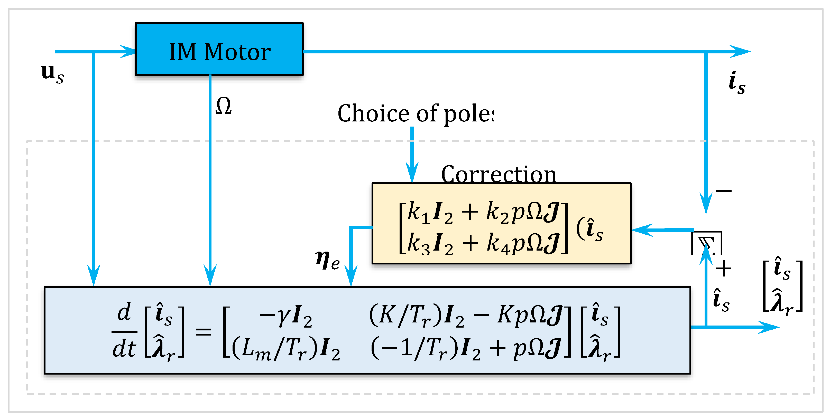
Figure 2.
The RBFNN Neural Networks Based Observer: Toward Intelligent Observation.
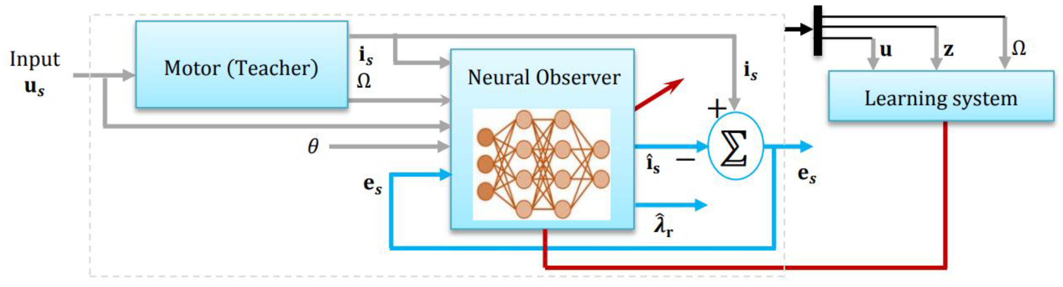
Figure 3.
Adaptation mechanism using a fuzzy logic observer.
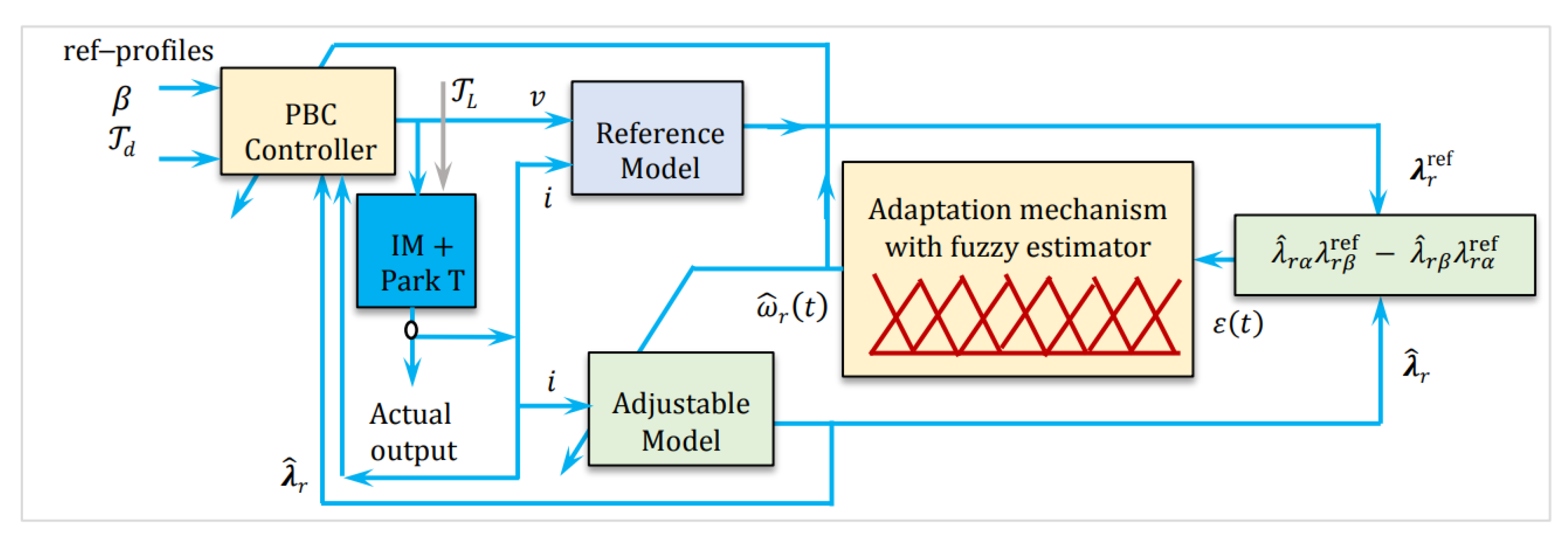
Figure 4.
Configuration of the Fuzzy Rule-Based Control Framework.
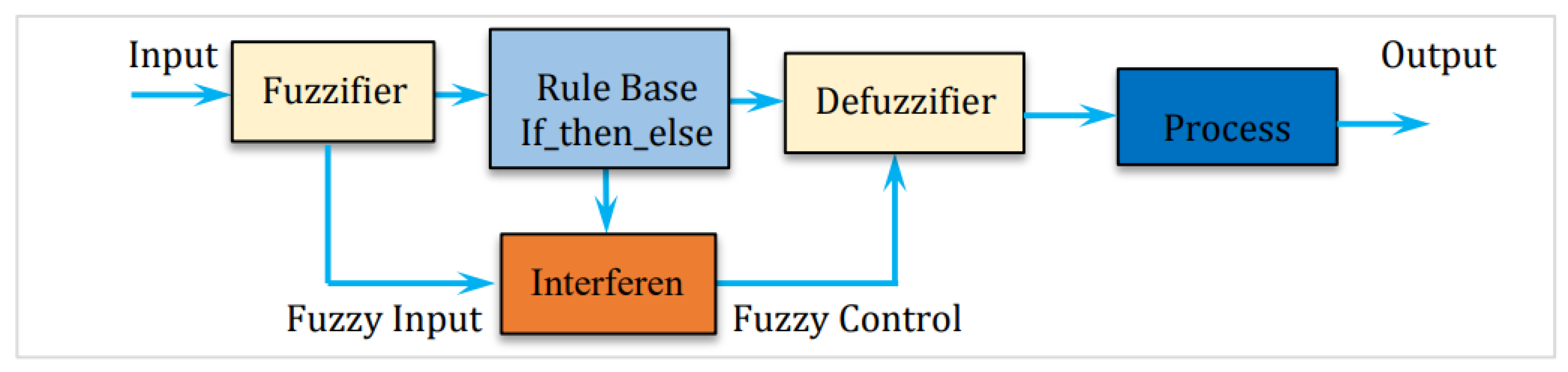
Figure 5.
Schematic Representation of the Fuzzy Logic Control System.
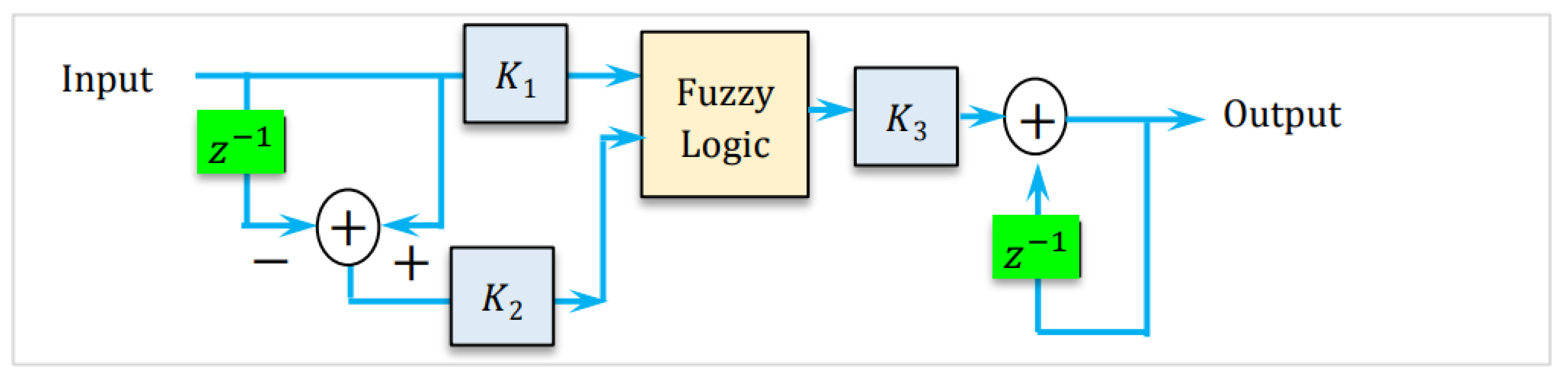
Figure 6.
Membership distribution of
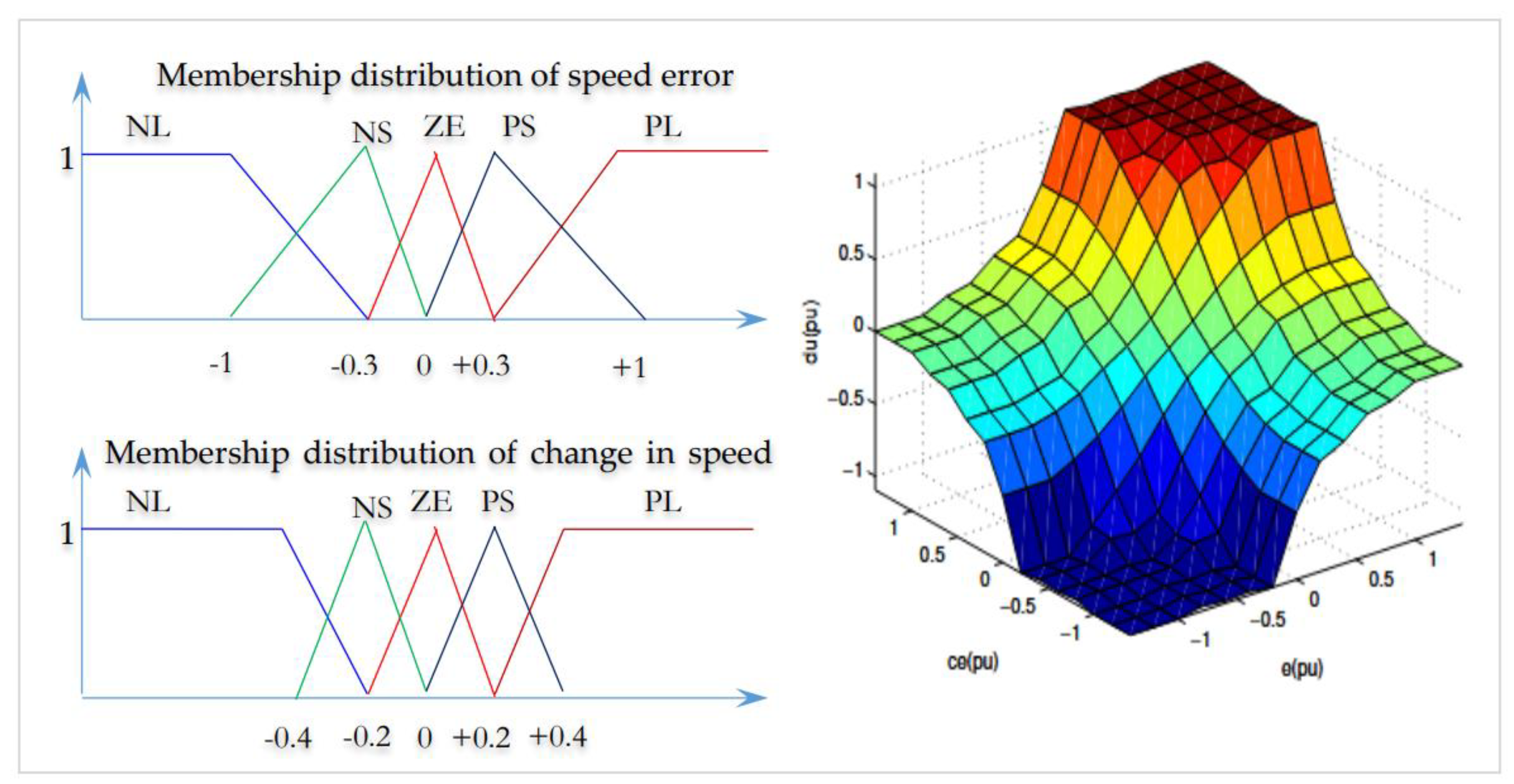
Figure 7.
Interaction of subsystems in IM motor.
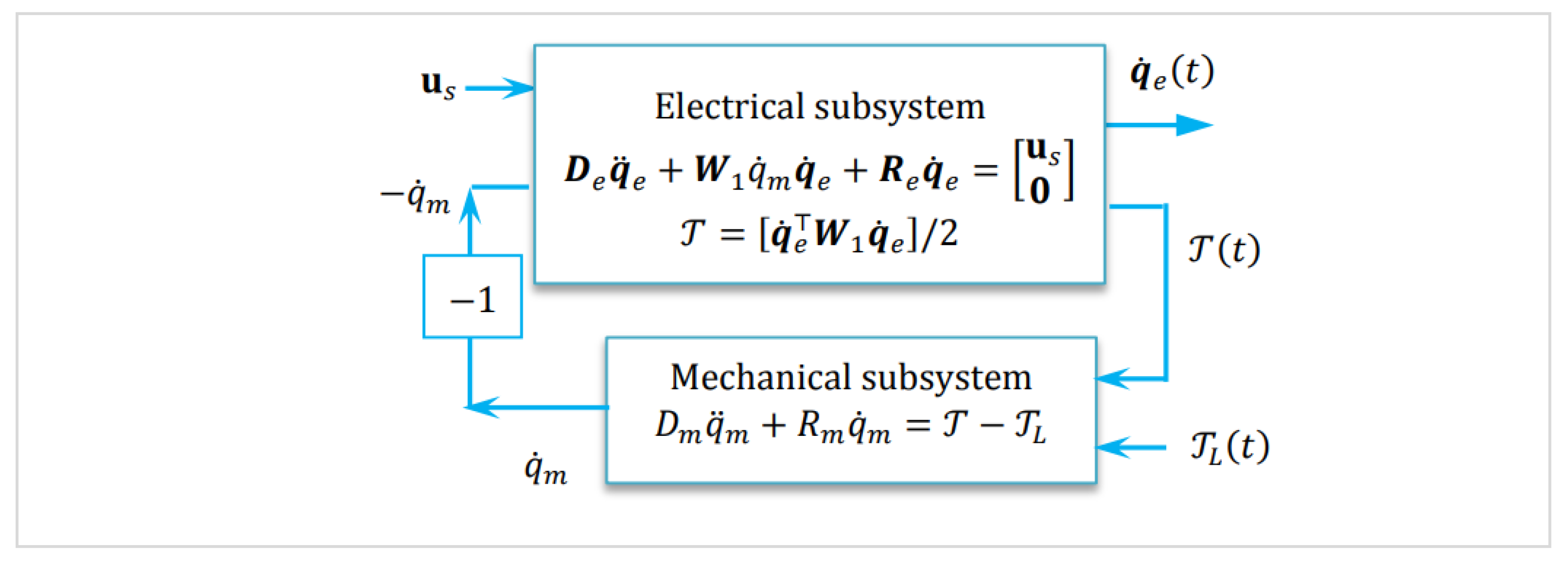
Figure 8.
Diagram of the Adaptive Sensorless Pasivity Control Scheme for Induction Motor Drive.
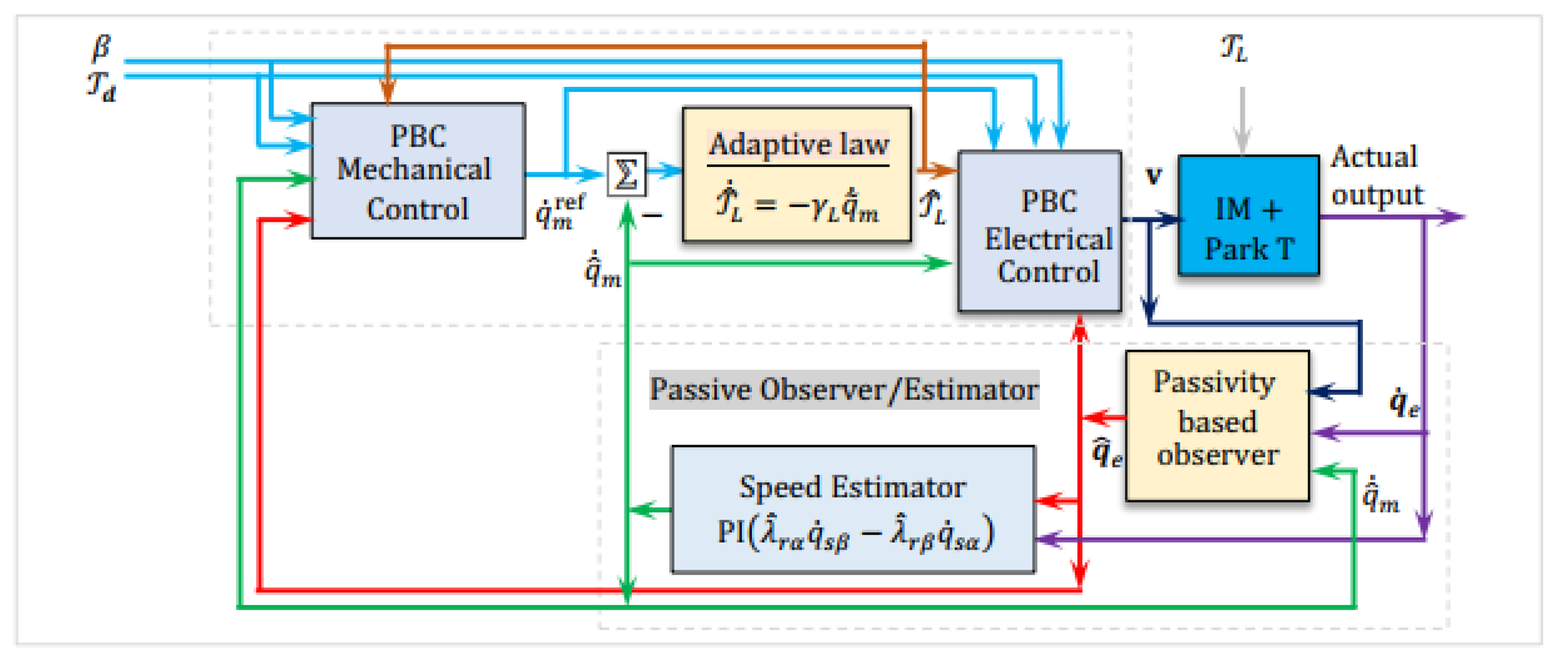
Figure 9.
Intelligent Adaptive Sensorless Pasivity Control Scheme for Induction Motor Drive.
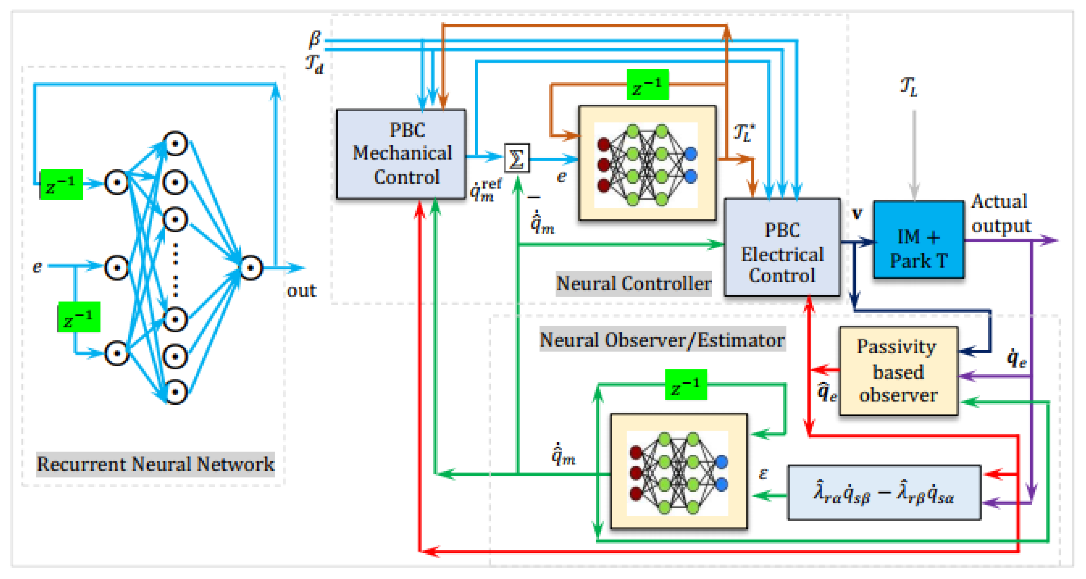
Figure 10.
Training Procedure of the RNN-Based Load Torque Estimator Using BPTT.
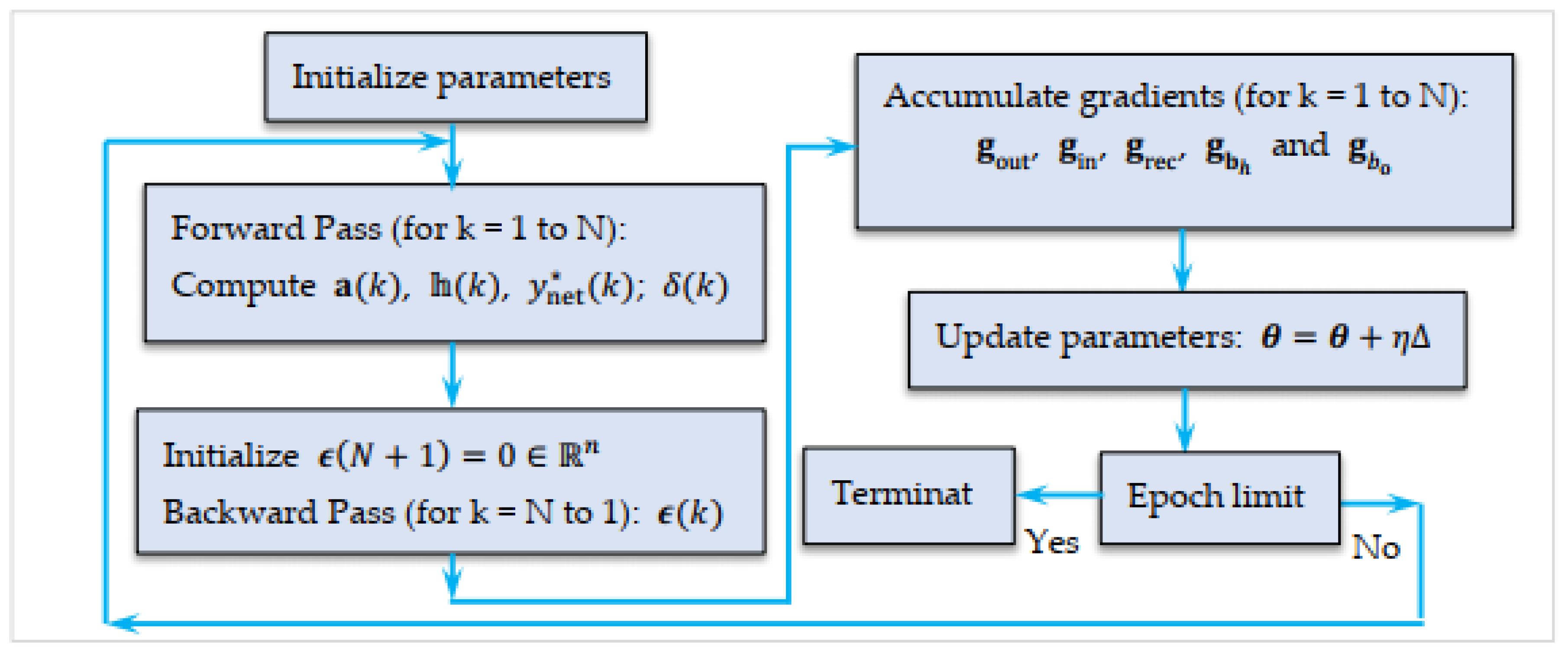
Figure 12.
Architecture of the Neural PBC Adaptive Control Scheme for Sensorless IMDrive.
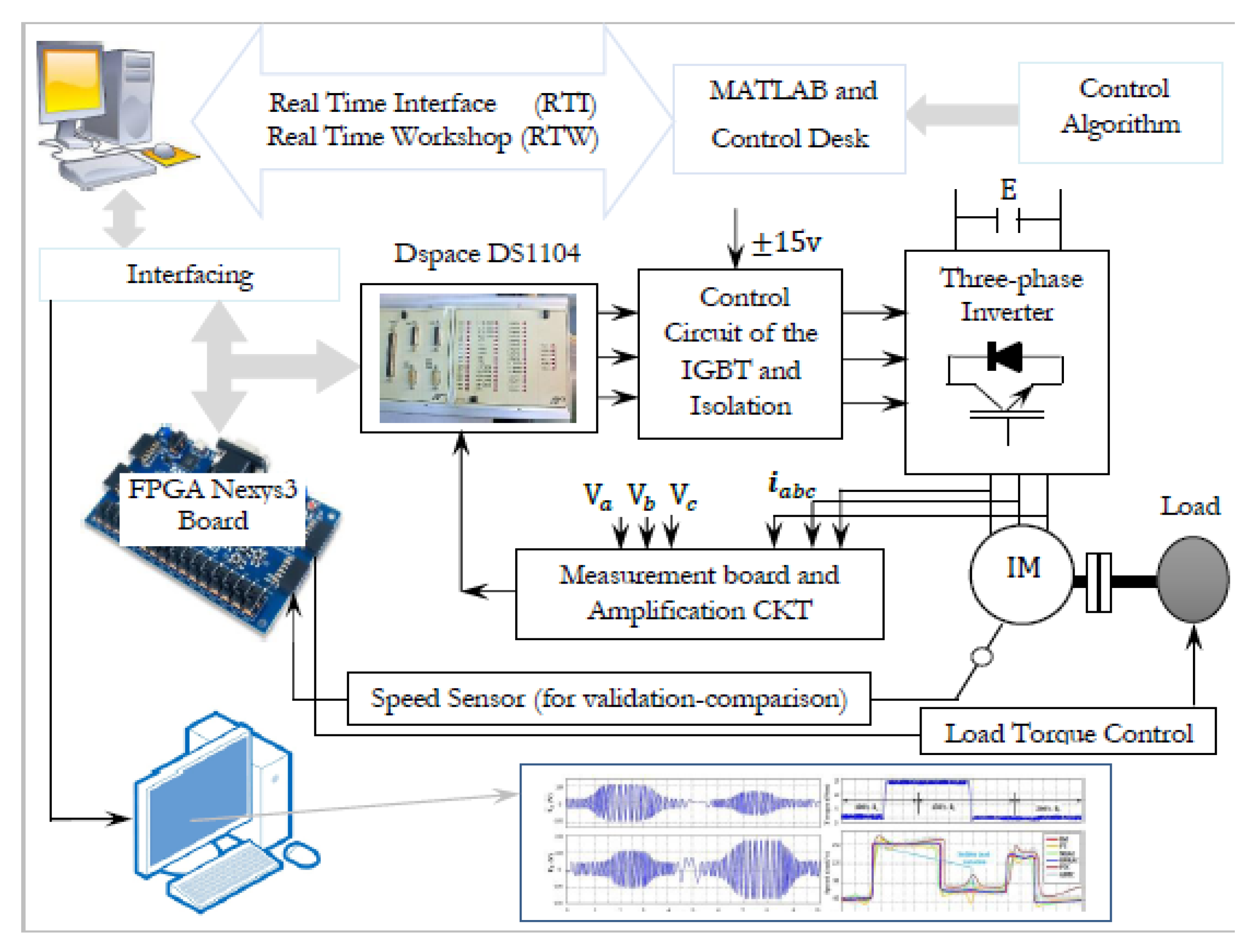
Figure 13.
Rotor Flux Observation Errors Via the Proposed Neural Nonlinear Observer.
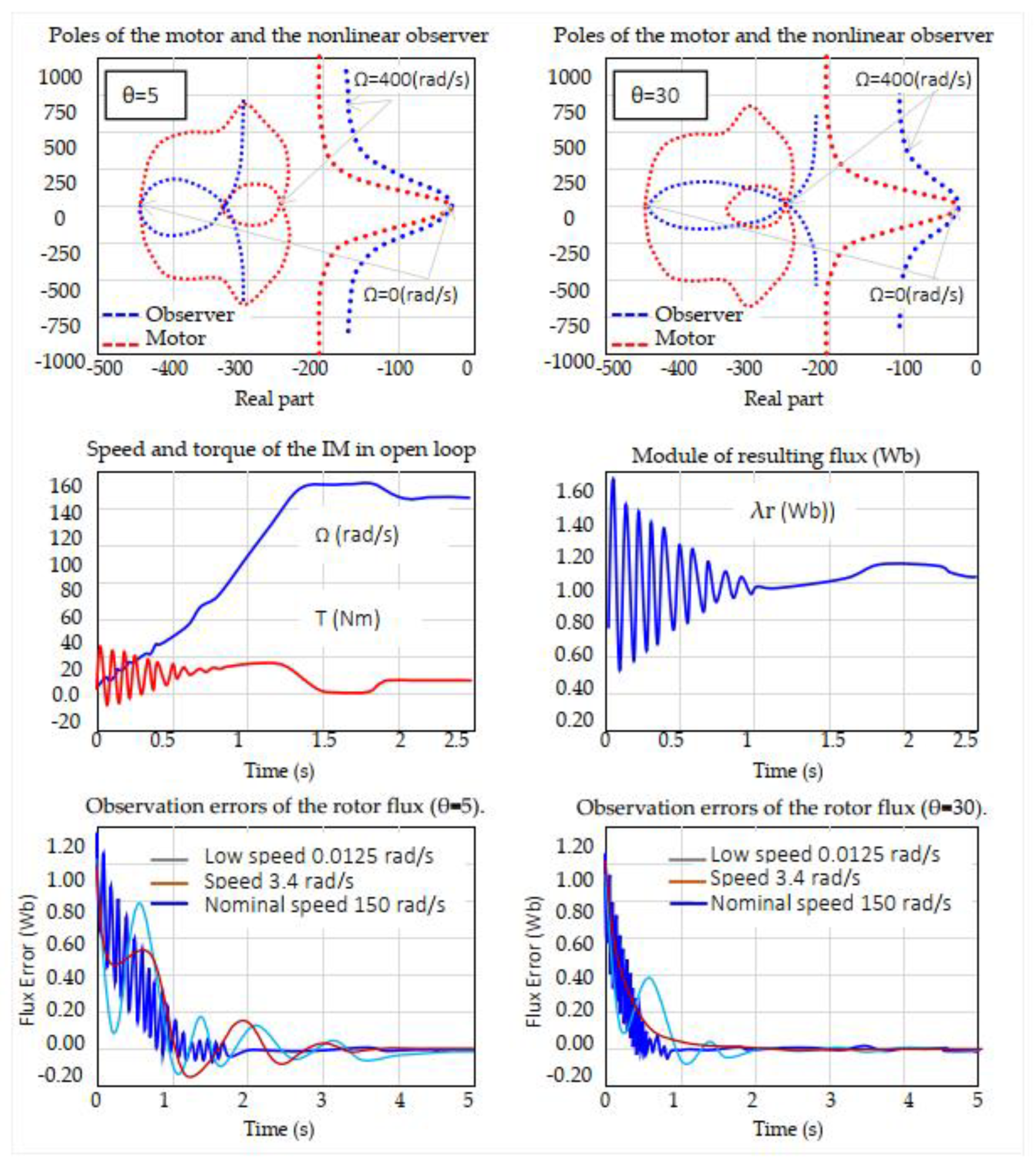
Figure 14.
Observer Convergence and Sensitivity Analysis Under Rotor Resistance Variations.
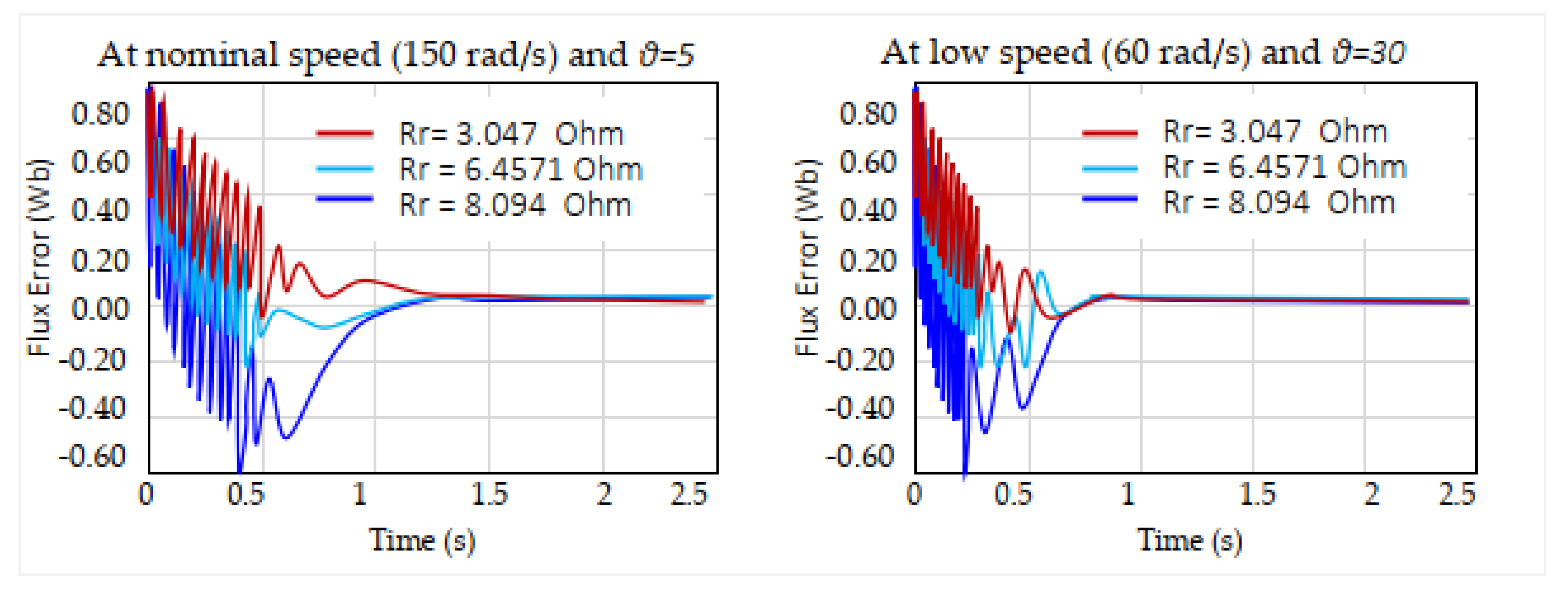
Figure 15.
Impact of RBFNN Compensation on Flux Estimation Robustness with
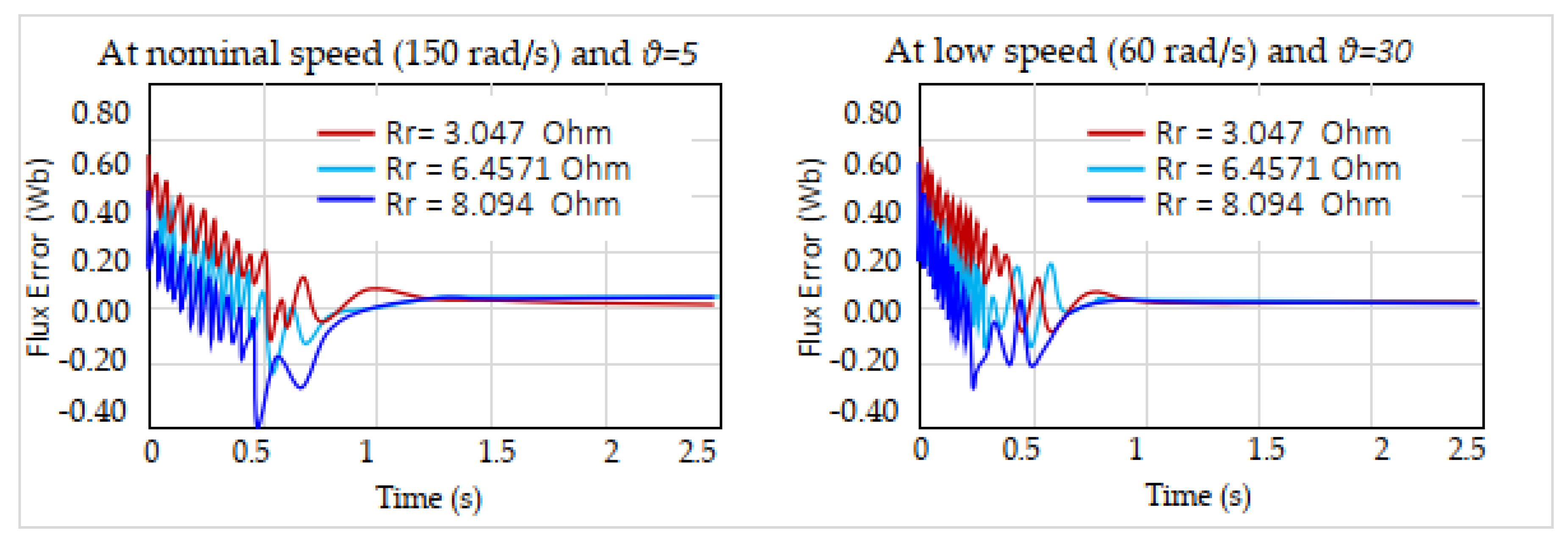
Figure 16.
Performance Study of the Proposed Control Scheme under Torque/Flux Variation.
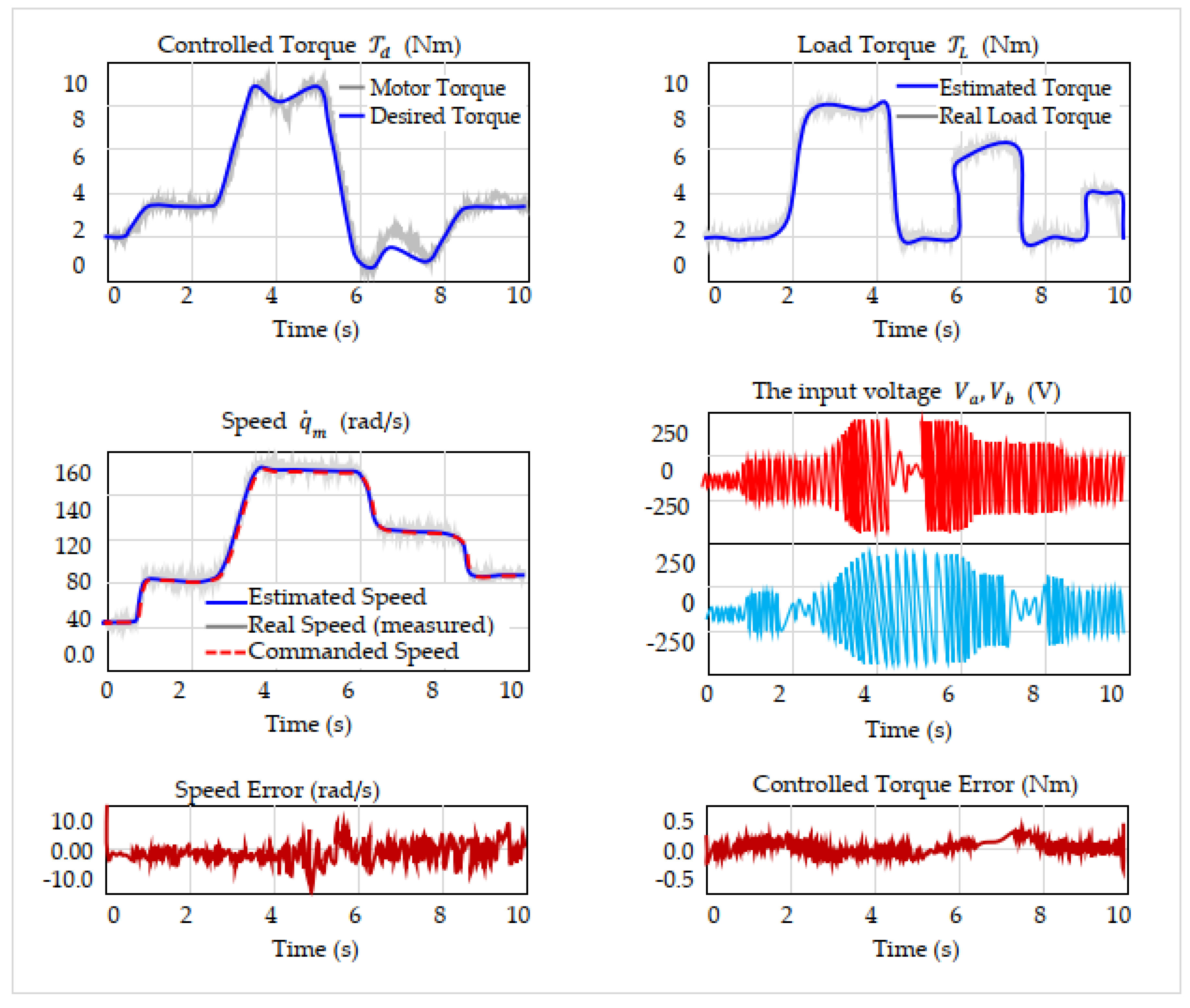
Figure 17.
Performance Study of the Proposed Control Scheme under Torque Reversal.
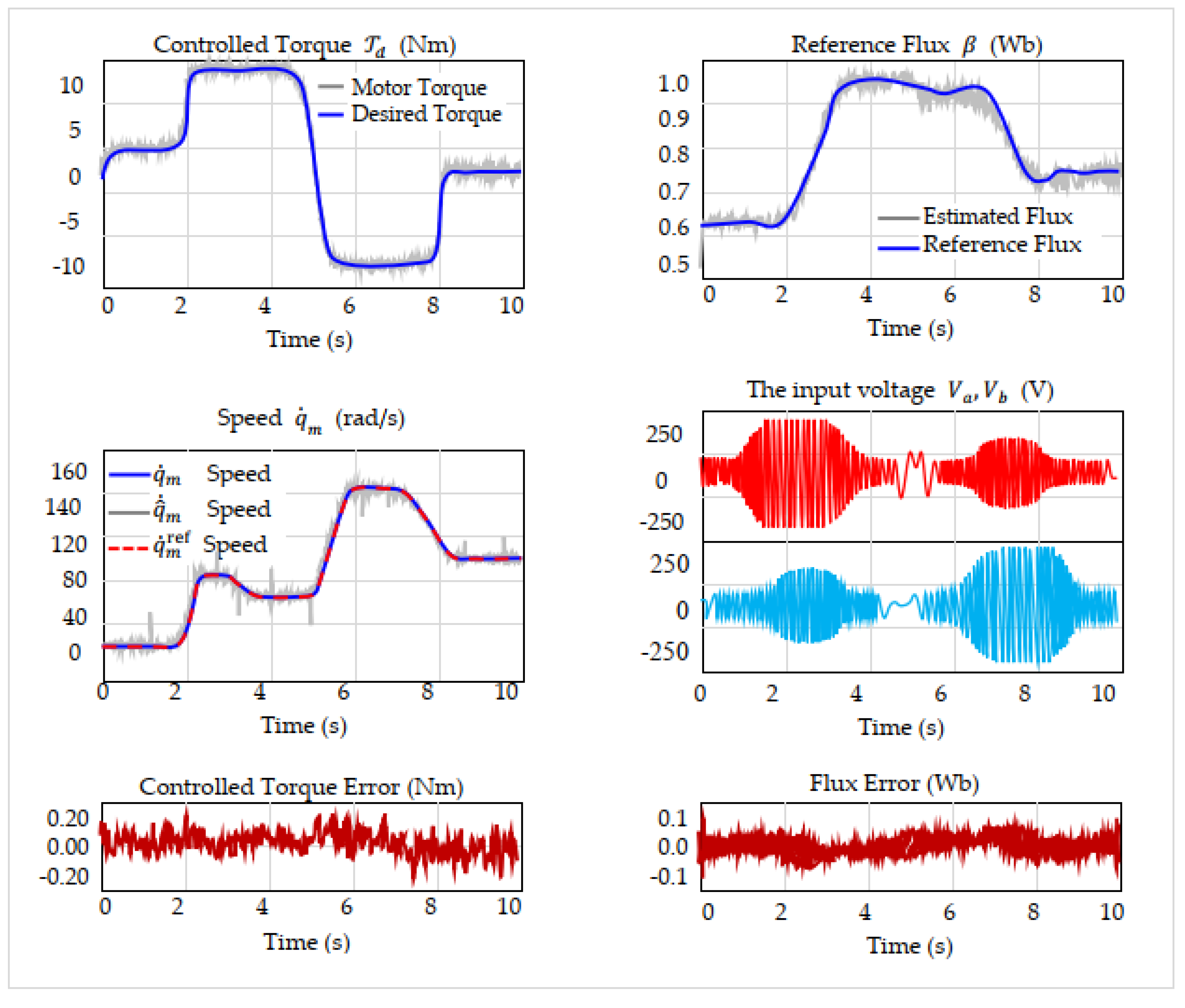
Figure 18.
Realistic Operating Conditions Benchmark Profiles for Comparative Study.
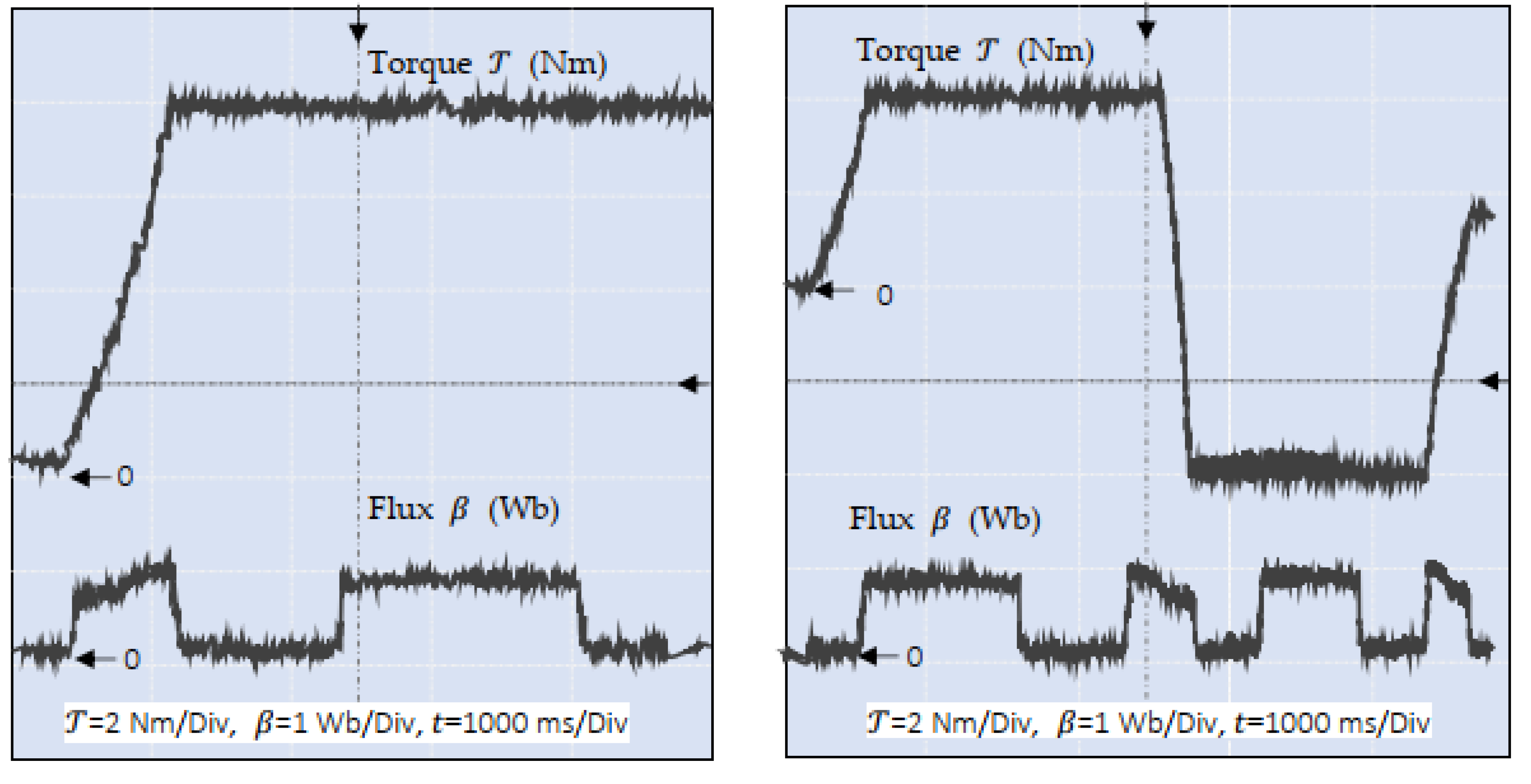

Table 1.
Fuzzy Rules for the Proposed System with a Rule Confidence Weights for Enhanced Inference
 |
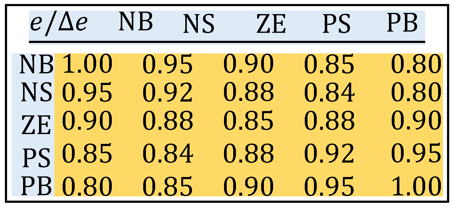 |
Table 2.
Induction Motor Parameters.
| Parameters name | Rating values | |
| • Stator resistance | 11.8 Ω | |
| • Rotor resistance | 11.3085 Ω | |
| • Mutual cyclic inductance | 0.5400 H | |
| • Stator cyclic inductance | 0.5578 H | |
| • Rotor cyclic inductance | 0.6152 H | |
| • Moment of inertia | 0.0020 Kg.m2 | |
| • Friction coefficient | 3.1165e-004 N.m/rad/s | |
| • Number of pair poles | 1 | |
Table 3.
Comparative Evaluation of Control Laws under Pseudo-Static Conditions.
| Torque () | Flux () | ||
| CNO-PBC | 0.68 21.40 | 16 882 0.49 1.92 0.73 36.83 | 0.47 44.33 |
| CFE-PBC | 0.15 17.35 | 18 861 0.21 1.08 0.26 30.40 | 0.22 35.95 |
| CRBF-PBC | 0.09 15.13 | 15 845 0.13 0.71 0.14 27.25 | 0.13 27.12 |
| DRNN-PBC | 0.06 14.23 | 13 825 0.08 0.43 0.05 24.81 | 0.10 21.92 |
| is ≈ 0.998 for all the used controller. | |||
Table 4.
Comparative Evaluation of Control Laws under Pseudo-Static Conditions.
| Torque () | Flux () | ||
| CNO-PBC | 1.58 26.12 | 18 1120 1.23 4.02 1.10 42.52 | 0.85 53.51 |
| CFE-PBC | 0.35 21.05 | 21 1005 0.65 2.31 0.41 36.51 | 0.41 39.54 |
| CRBF-PBC | 0.23 19.31 | 20 995 0.33 1.63 0.28 33.12 | 0.15 29.95 |
| DRNN-PBC | 0.18 18.52 | 19 985 0.27 1.13 0.21 30.85 | 0.21 28.63 |
| is ≈ 0.998 for all the used controller. | |||
Disclaimer/Publisher’s Note: The statements, opinions and data contained in all publications are solely those of the individual author(s) and contributor(s) and not of MDPI and/or the editor(s). MDPI and/or the editor(s) disclaim responsibility for any injury to people or property resulting from any ideas, methods, instructions or products referred to in the content. |
© 2025 by the authors. Licensee MDPI, Basel, Switzerland. This article is an open access article distributed under the terms and conditions of the Creative Commons Attribution (CC BY) license (http://creativecommons.org/licenses/by/4.0/).
Copyright: This open access article is published under a Creative Commons CC BY 4.0 license, which permit the free download, distribution, and reuse, provided that the author and preprint are cited in any reuse.


