Chronon Field Theory in 1+1 Dimensions: A Solvable Framework for Emergent Geometry, Gauge Fields, and Mass

1. Introduction

The quest to unify the fundamental structures of physics—geometry, matter, and gauge interactions—has long driven the development of theoretical frameworks beyond the Standard Model. Central to this pursuit is the challenge of formulating a theory in which these elements are not merely coexistent or coupled, but instead emerge coherently from a single underlying dynamical principle [26,33]. Chronon Field Theory (CFT) is one such proposal: a covariant field-theoretic framework in which spacetime geometry, gauge structure, inertial dynamics, and quantized matter arise from the behavior of a single, unit-norm timelike vector field.

The fundamental object in CFT is the Chronon field, denoted ${\mathrm{\Phi }}^{\mu }\left(x\right)$, defined on a Lorentzian manifold $(M,g_{\mu \nu })$ with signature $(-,+)$. This field satisfies the constraint $g_{\mu \nu }{\mathrm{\Phi }}^{\mu }{\mathrm{\Phi }}^{\nu }=-1$ and specifies a locally preferred, future-directed timelike direction at each spacetime point. Rather than assuming a background foliation or global time coordinate, CFT builds causal and geometric structure from the integral curves and orientation of ${\mathrm{\Phi }}^{\mu }$ itself. This perspective aligns with approaches in which spacetime and causality emerge from more primitive structures, such as quantum entanglement [46,48] or time-asymmetric flow fields [1].

An internal $U\left(1\right)$ phase, associated with the local frame ambiguity orthogonal to ${\mathrm{\Phi }}^{\mu }$, gives rise to an emergent gauge potential. Topologically nontrivial field configurations naturally carry conserved winding numbers, which correspond to quantized matter-like excitations. These features resonate with mechanisms in Kaluza–Klein theory [24,25], Cartan geometry [45], and tensor network models of holography [34], where internal geometric or topological degrees of freedom give rise to effective gauge fields and matter content.

While the full theory in 3+1 dimensions exhibits rich geometric and topological complexity, it is analytically intractable. To isolate and examine the core mechanisms of CFT, we consider a dimensionally reduced model in 1+1 dimensions. This reduced model retains all essential ingredients: a unit-norm Chronon field, emergent gauge structure from internal phase geometry, topological solitons with quantized charge, and a dynamically induced spacetime geometry. Crucially, the system is exactly solvable, allowing us to construct closed-form solutions, derive conserved quantities, and analyze linearized excitations around nontrivial backgrounds.

A central result of the 1+1D theory is that the concept of mass becomes physically multifaceted. Solitonic excitations exhibit three interrelated but distinct manifestations of mass: gradient mass (associated with spatial field energy), holonomy mass (arising from topological winding), and coherence mass (emergent from long-range phase rigidity). This mirrors the layered origin of hadronic mass in QCD, where the bulk of a particle’s mass arises dynamically rather than from its constituent quark masses. In the Chronon framework, these mass manifestations can differ, coincide, or even vanish in different regimes—suggesting the need for a generalized equivalence principle governing their dynamical role.

The reduced model thus functions not only as a pedagogical introduction to Chronon Field Theory, but as a rigorous and analytically tractable platform for testing its foundational claims. In this work, we present the complete formulation of 1+1D Chronon Field Theory, derive its exact solitonic and topological solutions, characterize the structure of emergent mass, and analyze the linear excitation spectrum in terms of photon- and graviton-like modes. These results lay a calculable foundation for understanding how matter, geometry, and gauge phenomena arise from Chronon dynamics in higher-dimensional settings.

2. Theoretical Context

The Chronon Field Theory (CFT) framework emerges at the intersection of several pivotal developments in modern theoretical physics. At its core, it proposes that spacetime, gauge fields, and matter degrees of freedom can be unified through the differential geometry of a single real vector field ${\mathrm{\Phi }}^{\mu }\left(x\right)$ subject to a unit-norm constraint. This approach resonates with a broader effort across quantum gravity, emergent spacetime models, and condensed matter analogs to recast conventional field-theoretic structures as emergent phenomena [23,26].

In particular, the idea that internal gauge symmetries can arise from geometrical or topological properties of spacetime (or of auxiliary field configurations) echoes earlier insights from Kaluza–Klein theory [24,25], fiber bundle formulations of gauge theory [32], and more recently, approaches such as emergent gravity from entanglement [48] and tensor network dualities [46]. However, unlike these frameworks, Chronon Field Theory maintains manifest covariance while deriving gauge interactions from the foliation and non-integrability structure induced by ${\mathrm{\Phi }}^{\mu }$, even in the absence of complex fields.

The 1+1 dimensional prototype developed in this paper serves both as a tractable mathematical model and a conceptual laboratory. In this reduced setting, one can isolate and rigorously study the emergence of $U\left(1\right)$ gauge structure, solitonic excitations, and multiple definitions of mass—elements that are essential to any realistic particle physics theory. The scalar field $\theta (x,t)$, which parametrizes the internal configuration space of ${\mathrm{\Phi }}^{\mu }$, becomes the linchpin for both geometric gauge emergence and the nonperturbative spectrum of excitations.

This framework is motivated in part by the longstanding challenge of explaining the mass hierarchy of elementary particles from first principles. While conventional quantum field theories treat mass parameters as inputs (subject to renormalization) [51], Chronon Field Theory aims to derive such parameters dynamically from topological, geometric, and coherent features of the underlying real-valued field structure. The richness of mass notions in 1+1D—gradient mass, holonomy mass, and coherence mass—provides a concrete starting point for this investigation.

In the long-term vision, higher-dimensional generalizations (e.g., 3+1D Chronon models) are expected to capture the full structure of the Standard Model gauge group and mass spectra. The current study thus represents the first step in a program to geometrize not only spacetime but also the origin of matter and its observable properties through real-valued differential geometry.

3. Chronon Field and Internal Geometry in 1+1D

We begin by formulating the Chronon Field Theory in the setting of a $(1+1)$-dimensional Lorentzian manifold $(M,g_{\mu \nu })$, where the metric signature is taken as $(-,+)$. The central dynamical object is a real-valued, future-directed timelike unit vector field ${\mathrm{\Phi }}^{\mu }\left(x\right)$, constrained by

$$g_{\mu \nu }{\mathrm{\Phi }}^{\mu }{\mathrm{\Phi }}^{\nu }=-1.$$

(1)

This condition endows spacetime with an intrinsic local time direction and replaces any externally imposed global clock with a covariant flow field. The vector ${\mathrm{\Phi }}^{\mu }$ generates a congruence of timelike integral curves that naturally define a foliation of spacetime into spatial hypersurfaces orthogonal to the temporal flow [5,50].

In $(1+1)$ dimensions, the unit-norm constraint restricts ${\mathrm{\Phi }}^{\mu }$ to lie on a one-dimensional hyperboloid $H^1\subset T_{x}M$, the space of unit timelike vectors at each point. This geometric constraint allows a canonical parametrization of ${\mathrm{\Phi }}^{\mu }$ in terms of a single real scalar field $\theta (x,t)$:

$${\mathrm{\Phi }}^{\mu }(x,t)=(cosh\theta (x,t),sinh\theta (x,t)),$$

(2)

which satisfies the normalization automatically:

$$-{cosh}^2\theta +{sinh}^2\theta =-1.$$

(3)

Here, $\theta (x,t)$ represents a local rapidity and serves as the sole dynamical degree of freedom in the theory. It encodes the internal orientation of ${\mathrm{\Phi }}^{\mu }$ with respect to a fixed Lorentz frame, and its configuration space inherits a natural hyperbolic geometry from the structure of $H^1$ [40].

Crucially, the scalar field $\theta (x,t)$ also induces an emergent gauge structure. The map

$$\theta :M^{1+1}\to S^1$$

(4)

defines a principal fiber bundle over spacetime, where the internal fiber $S^1$ corresponds to phase rotations of the vector ${\mathrm{\Phi }}^{\mu }$. The associated gauge potential

$$A_{\mu }:={\partial }_{\mu }\theta$$

(5)

acts as a connection on this bundle, transforming under local phase redefinitions $\theta \left(x\right)\mapsto \theta \left(x\right)+\alpha \left(x\right)$ as a $U\left(1\right)$ gauge field. This geometric interpretation parallels the emergence of gauge structures in theories based on nonlinear sigma models and spontaneous symmetry breaking [27,52].

In later sections, we will show that topologically nontrivial field configurations in $\theta$ yield quantized charges and solitonic excitations, which form the building blocks of emergent matter in this framework. Such solitonic structures are well-studied in low-dimensional field theory and provide a tractable setting for exploring mass quantization and coherence effects [39].

3.1. Frobenius Theorem and Foliation Structure

Even in the reduced context of $(1+1)$ dimensions, the foliation structure induced by ${\mathrm{\Phi }}^{\mu }$ benefits from a rigorous geometric foundation. Frobenius’ theorem provides a necessary and sufficient condition for a smooth distribution of vector fields to be integrable—that is, to define a family of non-intersecting hypersurfaces.

To apply this, consider the spatial distribution $\mathcal{D}$ orthogonal to ${\mathrm{\Phi }}^{\mu }$, defined via the projection tensor

$$h_{\mu \nu }:=g_{\mu \nu }+{\mathrm{\Phi }}_{\mu }{\mathrm{\Phi }}_{\nu },$$

(6)

which satisfies $h_{\mu \nu }{\mathrm{\Phi }}^{\nu }=0$. Frobenius’ theorem states that $\mathcal{D}$ is integrable if and only if the Lie bracket of any pair of vector fields within $\mathcal{D}$ remains in $\mathcal{D}$. In terms of differential forms, this condition is equivalent to the vanishing of the torsion-like 2-form constructed from ${\mathrm{\Phi }}^{♭}$:

$${\mathrm{\Phi }}_{[\mu }{\nabla }_{\nu }{\mathrm{\Phi }}_{\rho ]}=0.$$

(7)

In the $(1+1)$-dimensional setting, this integrability condition is automatically satisfied for smooth field configurations, and hence ${\mathrm{\Phi }}^{\mu }$ always induces a well-defined foliation of spacetime into spatial slices. However, when $\theta (x,t)$ acquires topological defects, such as domain walls or solitons, the orthogonal distribution can become non-integrable in localized regions. These points of breakdown correspond to singularities in the foliation, which in turn source holonomy and topological effects in the emergent gauge structure.

Thus, Frobenius theory serves two roles: it ensures the existence of spatial hypersurfaces in the smooth regime and offers a precise geometric language for describing singular configurations where the foliation breaks down. These singularities play a critical role in the emergence of gauge and matter structures from internal geometry.

4. Action and Field Equations

To formulate the dynamics of the Chronon field in $1+1$ dimensions, we construct a covariant action in terms of the scalar field $\theta (x,t)$ which parametrizes the timelike unit vector ${\mathrm{\Phi }}^{\mu }$ [15,50]. As established, the Chronon vector is given by

$${\mathrm{\Phi }}^{\mu }=(cosh\theta ,sinh\theta ),$$

(8)

and its derivatives encode the deformation and curvature of the local temporal flow [13,14].

We define the Lagrangian density for the reduced Chronon Field Theory as

$$\mathcal{L}(\theta ,{\partial }_{\mu }\theta )={\displaystyle \frac{1}{2}}cosh\left(2\theta \right){\partial }_{\mu }\theta {\partial }^{\mu }\theta -V\left(\theta \right),$$

(9)

where the first term captures the kinetic energy weighted by a geometric prefactor $cosh\left(2\theta \right)$ arising from the embedding of the hyperbolic field manifold [55], and $V\left(\theta \right)$ is a potential that allows for topologically distinct vacuum sectors.

A natural and widely studied choice for $V\left(\theta \right)$ is the sine-Gordon potential [7,38],

$$V\left(\theta \right)={\mu }^2(1-cos\theta ),$$

(10)

where $\mu$ is a real constant with dimensions of mass. This potential admits an infinite set of degenerate vacua at $\theta =2\pi n$, $n\in \mathbb{Z}$, enabling the existence of kink-type solitonic solutions that interpolate between distinct vacua [9].

To obtain the Euler–Lagrange equations, we vary the action

$$S\left[\theta \right]=\int d^{2}x\mathcal{L}(\theta ,{\partial }_{\mu }\theta )$$

(11)

with respect to $\theta$. This yields the equation of motion:

$$cosh\left(2\theta \right)\square \theta +sinh\left(2\theta \right){\partial }_{\mu }\theta {\partial }^{\mu }\theta +{\mu }^{2}sin\theta =0,$$

(12)

where $\square ={\partial }_{\mu }{\partial }^{\mu }$ is the d’Alembertian operator in flat spacetime.

This equation is a nonlinear wave equation for $\theta (x,t)$, with both field-dependent kinetic terms and a nonlinear source from the sine-Gordon potential. As we will show, it admits exact static solutions corresponding to solitons [12], and supports linear perturbations that give rise to emergent gauge and gravitational phenomena [32].

The potential $V\left(\theta \right)$ plays a crucial role in defining the topological sectors of the theory. Since the vacua are labeled by integers $n\in \mathbb{Z}$, field configurations with asymptotic behavior

$$\underset{x\to -\infty }{lim}\theta \left(x\right)=2\pi n,\underset{x\to +\infty }{lim}\theta \left(x\right)=2\pi m,$$

(13)

are classified by the winding number $Q=m-n\in \mathbb{Z}$, which will be identified with the conserved topological (electric) charge in later sections [27].

4.1. Origin and Interpretation of the Parameter $\mu$

The parameter $\mu$ enters the theory as the characteristic scale appearing in the effective potential governing the internal phase field $\theta (x,t)$, such as

$$V\left(\theta \right)={\mu }^2(1-cos\theta ),$$

(14)

or its generalizations [7,37]. Physically, $\mu$ sets the inverse width and energy scale of localized soliton solutions, and thus determines both the gradient energy and coherence length in static configurations. Therefore $\mu$ is interpreted as the mass scale parameter.

From a theoretical perspective, $\mu$ may be interpreted in multiple ways, depending on the origin of the effective action:

• If the Chronon field theory is taken as fundamental, $\mu$ is an input parameter specifying the curvature of the potential near its minimum [55].
• If the theory arises as a low-energy effective description of a deeper microscopic model, $\mu$ could be a dynamically generated scale via dimensional transmutation or quantum anomaly (e.g., in analogy with the QCD scale ${\Lambda }_{\mathrm{QCD}}$) [3,17].
• Under renormalization group flow, $\mu$ can be viewed as a renormalized parameter: the only relevant scale left after integrating out UV degrees of freedom, giving the effective mass gap of the system [56].

In all interpretations, $\mu$ controls the mass scale of excitations, the energy density of solitons, and the rate of exponential decay in correlation functions (i.e., coherence mass). It serves as the unifying parameter across the gradient, holonomy, and coherence mass definitions presented in this work. When comparing different composite configurations, mass ratios are expressed as dimensionless multiples of $\mu$, enabling a hierarchy analysis independent of absolute scale.

5. Soliton Solutions and Emergent Matter

We now consider static, finite-energy solutions of the field equations derived in the previous section. Such solutions correspond to topologically nontrivial interpolations between degenerate vacua of the potential $V\left(\theta \right)$. In the sine-Gordon case, these are kink-type solitons [12,38].

Assuming time-independence, the equation of motion reduces to

$${\displaystyle \frac{d^2\theta }{d{x}^2}}={\displaystyle \frac{{\mu }^{2}sin\theta }{cosh\left(2\theta \right)}}.$$

(15)

While this nonlinear second-order equation cannot be integrated in closed form in general, one can find an exact solution in the special case where the kinetic prefactor is treated approximately as constant near the vacuum sectors [9]. However, it is more instructive to consider a modified equation in which the standard sine-Gordon kink is also a solution. This occurs when the Lagrangian is taken to be

$${\mathcal{L}}_{\mathrm{SG}}={\displaystyle \frac{1}{2}}{\partial }_{\mu }\theta {\partial }^{\mu }\theta -{\mu }^2(1-cos\theta ),$$

(16)

which describes the well-known sine-Gordon model [7].

The corresponding static equation is

$${\displaystyle \frac{d^2\theta }{d{x}^2}}={\mu }^{2}sin\theta .$$

(17)

This admits the well-known kink solution:

$$\theta \left(x\right)=4{tan}^{-1}\left(e^{\mu (x-x_0)}\right),$$

(18)

which interpolates between $\theta =0$ as $x\to -\infty$ and $\theta =2\pi$ as $x\to +\infty$ [38]. Here $x_0$ is an arbitrary constant corresponding to the position of the soliton.

This solution defines a field configuration with winding number $Q=1$, and as we will now show, this topological charge corresponds to an emergent conserved quantity interpreted as electric charge in the Chronon framework. Define the topological current

$$J^{\mu }={\displaystyle \frac{1}{2\pi }}{ϵ}^{\mu \nu }{\partial }_{\nu }\theta ,$$

(19)

which is identically conserved:

$${\partial }_{\mu }{J}^{\mu }=0.$$

(20)

The associated conserved quantity is the topological charge

$$Q=\int dx{J}^0={\displaystyle \frac{1}{2\pi }}\int dx{\partial }_x\theta ={\displaystyle \frac{1}{2\pi }}[\theta (+\infty )-\theta (-\infty )]\in \mathbb{Z},$$

(21)

which is naturally interpreted as electric charge in the emergent $U\left(1\right)$ structure [27].

Next, we define the energy of a static field configuration as

$$E=\int dx\left[{\displaystyle \frac{1}{2}}{\left({\displaystyle \frac{d\theta }{dx}}\right)}^2+V\left(\theta \right)\right].$$

(22)

For the sine-Gordon kink solution, one finds

$$E=8\mu ,$$

(23)

independent of $x_0$, confirming the translational invariance of the soliton [9,12]. This energy is interpreted as the mass of the emergent matter excitation, arising entirely from deformation of the Chronon field.

We thus obtain a complete picture of particle emergence in 1+1D Chronon Field Theory: topological solitons in the internal phase $\theta \left(x\right)$ behave as localized, massive, quantized excitations carrying conserved electric charge. These entities arise solely from the field’s geometry, with no need to postulate additional particle degrees of freedom.

5.1. Intrinsic Origin of Mass and Charge

One of the most striking features of the Chronon Field Theory (CFT) in 1+1 dimensions is that both mass and electric charge arise intrinsically from the internal geometry of the field, without invoking external gauge symmetries or symmetry-breaking mechanisms such as the Higgs field [53].

In conventional field theory, the mass of elementary particles is typically generated via the Higgs mechanism, which introduces a scalar field coupled to matter through Yukawa interactions [35]. This mechanism requires spontaneous symmetry breaking and an external scalar sector, and the values of particle masses are encoded in a set of arbitrary coupling constants. Similarly, electric charge is introduced as a fixed quantum number assigned to fields that transform under a $U\left(1\right)$ gauge symmetry. Its magnitude and quantization are not derived from first principles but treated as empirical input [51].

In CFT, the situation is fundamentally different. The Chronon field is a unit-norm timelike vector field parametrized by an internal phase $\theta (x,t)$. The nontrivial topology of the field configuration space, specifically the nontrivial homotopy group ${\pi }_1\left(U\left(1\right)\right)=\mathbb{Z}$, gives rise to solitonic solutions—kinks—that interpolate between neighboring vacua in the target space [27].

These solitons are classified by their winding number:

$$Q={\displaystyle \frac{1}{2\pi }}{\int }_{-\infty }^{\infty }{\partial }_x\theta \left(x\right)dx\in \mathbb{Z},$$

(24)

which is naturally interpreted as electric charge in the emergent $U\left(1\right)$ gauge structure [42].

The mass of these excitations is not inserted by hand but arises as the deformation energy of the background Chronon field required to sustain a topological transition. As shown in the appendix, the energy of the sine-Gordon kink solution is finite and given by

$$m=E_{\mathrm{kink}}=8\mu ,$$

(25)

where $\mu$ is the coupling constant in the potential term $V\left(\theta \right)={\mu }^2(1-cos\theta )$. Thus, mass is identified with the integrated tension of the field geometry and does not require coupling to an external scalar field.

This derivation situates both electric charge and rest mass as emergent, intrinsic properties of the geometric structure of the Chronon field. It demonstrates that fundamental physical quantities typically introduced as external inputs in standard models can, within the CFT framework, be understood as natural consequences of field topology and internal geometry. This elevates CFT from a model of unification to a foundational framework for understanding the origin of conserved quantum numbers in physics.

6. Emergent Geometry and Gravity

The Chronon field ${\mathrm{\Phi }}^{\mu }$ not only encodes a preferred temporal direction, but also induces a notion of local spatial geometry. In $1+1$ dimensions, the spacetime metric $g_{\mu \nu }$ can be decomposed with respect to ${\mathrm{\Phi }}^{\mu }$ as

$$g_{\mu \nu }=-{\mathrm{\Phi }}_{\mu }{\mathrm{\Phi }}_{\nu }+h_{\mu \nu },$$

(26)

where $h_{\mu \nu }$ is a rank-one projection tensor orthogonal to ${\mathrm{\Phi }}^{\mu }$:

$$h_{\mu \nu }{\mathrm{\Phi }}^{\nu }=0,h_{\mu \nu }=g_{\mu \nu }+{\mathrm{\Phi }}_{\mu }{\mathrm{\Phi }}_{\nu }.$$

(27)

This decomposition is standard in the analysis of timelike congruences and forms the basis of the ADM and Landau–Lifshitz formalisms [18,29,50].

The tensor $h_{\mu \nu }$ projects onto the spatial direction as seen by an observer moving with velocity ${\mathrm{\Phi }}^{\mu }$. The line element experienced by such an observer is

$$d{s}^2=h_{\mu \nu }d{x}^{\mu }d{x}^{\nu },$$

(28)

which defines an effective spatial metric field induced by the Chronon configuration [4,13].

Moreover, the covariant derivative of the Chronon field defines an acceleration vector field:

$$a^{\mu }={\mathrm{\Phi }}^{\nu }{\nabla }_{\nu }{\mathrm{\Phi }}^{\mu },$$

(29)

which measures the deviation of ${\mathrm{\Phi }}^{\mu }$ from geodesic flow. In flat spacetime, this reduces to

$$a^{\mu }={\mathrm{\Phi }}^{\nu }{\partial }_{\nu }{\mathrm{\Phi }}^{\mu },$$

(30)

as standard for congruence kinematics [36]. This acceleration field depends explicitly on derivatives of the internal phase $\theta (x,t)$ and encodes the intrinsic curvature of the Chronon congruence. It thus serves as an effective gravitational field, analogous to the role played by the expansion, shear, and vorticity in the Raychaudhuri equation [36,50].

The motion of test particles is governed by the effective geodesic equation in the induced geometry. In particular, the force experienced by a particle comoving with ${\mathrm{\Phi }}^{\mu }$ is given by the projection of $a^{\mu }$ onto the spatial subspace, leading to effective gravitational dynamics [4]. In the vicinity of a soliton, where $\theta \left(x\right)$ varies rapidly, $a^{\mu }$ is nonzero and localized, mimicking a gravitational well centered at the kink [22]. Hence, matter deformations in the Chronon field generate not only mass and charge, but also induce spacetime curvature, providing a unified origin for both gauge and gravitational phenomena [2,49].

7. Emergent Gauge Structure

In addition to inducing spacetime geometry, the internal phase $\theta (x,t)$ of the Chronon field also acts as an effective $U\left(1\right)$ gauge degree of freedom. The derivative

$$A_{\mu }={\partial }_{\mu }\theta$$

(31)

is interpreted as an emergent gauge potential, locally defined and transforming as a connection under internal phase reparametrizations [31,42]. Although the theory involves no explicit gauge group, the topology of the configuration space introduces an effective $U\left(1\right)$ structure [13,27].

Since the vacuum manifold is the circle $S^1$, the space of finite-energy configurations admits nontrivial first homotopy group:

$${\pi }_1\left(S^1\right)=\mathbb{Z}.$$

(32)

This leads to quantized winding numbers associated with the field $\theta \left(x\right)$, which we have already seen correspond to conserved charges carried by solitons [7,51]. Thus, the quantization of electric charge arises from the topological classification of field configurations, rather than from the imposition of discrete quantum numbers.

Furthermore, one may define a Noether current associated with global shifts of $\theta$:

$$j^{\mu }=cosh\left(2\theta \right){\partial }^{\mu }\theta ,$$

(33)

which is conserved in the absence of a potential. However, in the presence of a nontrivial $V\left(\theta \right)$, only the topological current

$$J^{\mu }={\displaystyle \frac{1}{2\pi }}{ϵ}^{\mu \nu }{\partial }_{\nu }\theta$$

(34)

is identically conserved and associated with a robust, quantized charge [21].

Altogether, the internal structure of the Chronon field gives rise to an emergent $U\left(1\right)$ gauge potential, quantized electric charges, and conserved currents, all derived from the geometry of a single unit-norm vector field. The resulting gauge sector arises not from symmetry imposition, but from the intrinsic topology and differential structure of the Chronon configuration space [22].

7.1. Geometric Origin of $U\left(1\right)$ via Holonomy

In the Chronon Field Theory framework, the emergent $U\left(1\right)$ gauge structure arises not from imposing a local symmetry in the conventional sense, but from the internal geometry of the Chronon field itself. Specifically, the internal phase $\theta (x,t)$ defines a map from spacetime into the circle $S^1$, and the variation of $\theta$ along paths induces a natural notion of holonomy that mimics a gauge connection [31,55].

The origin of this internal phase $\theta$ lies in the unit-norm constraint imposed on the Chronon field ${\mathrm{\Phi }}^{\mu }\left(x\right)$, which satisfies

$$g_{\mu \nu }{\mathrm{\Phi }}^{\mu }\left(x\right){\mathrm{\Phi }}^{\nu }\left(x\right)=-1.$$

(35)

This condition restricts ${\mathrm{\Phi }}^{\mu }$ to lie on a target manifold — the unit hyperboloid $H^n\subset T_{x}M$ in the tangent space at each spacetime point x. In 1+1 dimensions, this reduces to a 1D manifold isomorphic to $S^1$, enabling a parametrization in terms of a single angular degree of freedom:

$${\mathrm{\Phi }}^{\mu }\left(x\right)=(cos\theta \left(x\right),sin\theta \left(x\right)).$$

(36)

Thus, $\theta (x,t)$ emerges as an intrinsic scalar field that captures the internal orientation of the unit vector ${\mathrm{\Phi }}^{\mu }$. Its variation over spacetime provides a natural fiber bundle structure:

$$\theta :M^{1+1}\to S^1,$$

(37)

with $S^1$ as the internal fiber over each spacetime point [30].

Because Chronon Field Theory defines an irreversible time direction through ${\mathrm{\Phi }}^{\mu }$, conventional geometric holonomy around closed spacetime loops must be generalized. In this context, the relevant notion of holonomy can arise in three ways:

(i)

In compactified spatial geometries (e.g., $x\in S^1$), one can define closed loops along space at fixed time. The integral of ${\partial }_x\theta$ around such loops gives quantized winding numbers and associated topological charges [27].

(ii)

In non-compact space, global soliton solutions still lead to well-defined topological holonomy:

$$\Delta \theta ={\int }_{-\infty }^{\infty }{\partial }_x\theta \left(x\right)dx,$$

(38)

which classifies field configurations into homotopy sectors.

(iii)

On infinitesimal scales, one can compute holonomy over parallelograms spanned by $d{x}^{\mu }$ and $dt$, even without literal loop closure in time. This captures the curvature of the emergent $U\left(1\right)$ connection via

$$F_{\mu \nu }={\partial }_{\mu }{A}_{\nu }-{\partial }_{\nu }{A}_{\mu }.$$

(39)

Let $\gamma$ be a path in spacetime. The internal phase $\theta (x,t)$ defines a lift into $S^1$, and the holonomy associated with $\gamma$ is the net change in $\theta$ along this path:

$$\Delta \theta ={\int }_{\gamma }{\partial }_{\mu }\theta d{x}^{\mu }={\int }_{\gamma }{A}_{\mu }d{x}^{\mu }.$$

(40)

This is structurally identical to a Wilson line in gauge theory [35]. The field $A_{\mu }:={\partial }_{\mu }\theta$ behaves as a pure gauge connection on a principal $U\left(1\right)$-bundle over spacetime, with gauge symmetry

$$\theta \left(x\right)\mapsto \theta \left(x\right)+\alpha \left(x\right),A_{\mu }\mapsto A_{\mu }+{\partial }_{\mu }\alpha .$$

(41)

Although the local field $A_{\mu }$ remains pure gauge in trivial topological sectors, soliton solutions induce nontrivial holonomy that becomes physically observable as quantized electric charge [21].

This construction shows that the emergent $U\left(1\right)$ gauge structure is not merely an artifact of reparametrization, but a geometrically meaningful quantity arising from the global and local properties of the Chronon field. It sets the stage for a unified understanding of gauge interactions as holonomic effects of internal geometry, consistent with the interpretation in higher-dimensional generalizations of CFT [22,53].

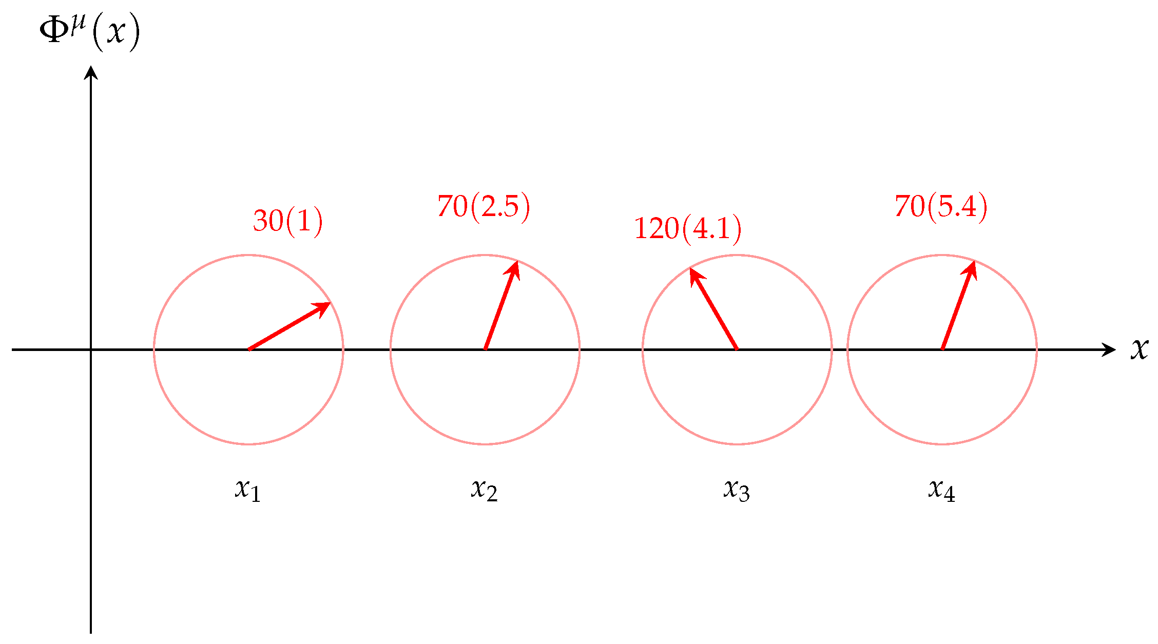
Figure 1. Visualization of the internal angle $\theta \left(x\right)$ at different spatial points in 1+1D Chronon Field Theory. Each circle represents the internal fiber $S^1$ attached to the base spacetime manifold at position $x_i$, and the red arrows show the orientation of the unit-norm vector ${\mathrm{\Phi }}^{\mu }\left(x_i\right)=(cos\theta \left(x_i\right),sin\theta \left(x_i\right))$ within the internal space. The angle $\theta \left(x\right)$ is not a spacetime coordinate but an internal degree of freedom that varies smoothly across spacetime, defining a bundle map $\theta :M^{1+1}\to S^1$. This internal structure underlies the emergent $U\left(1\right)$ gauge connection associated with phase holonomy.

Figure 1. Visualization of the internal angle $\theta \left(x\right)$ at different spatial points in 1+1D Chronon Field Theory. Each circle represents the internal fiber $S^1$ attached to the base spacetime manifold at position $x_i$, and the red arrows show the orientation of the unit-norm vector ${\mathrm{\Phi }}^{\mu }\left(x_i\right)=(cos\theta \left(x_i\right),sin\theta \left(x_i\right))$ within the internal space. The angle $\theta \left(x\right)$ is not a spacetime coordinate but an internal degree of freedom that varies smoothly across spacetime, defining a bundle map $\theta :M^{1+1}\to S^1$. This internal structure underlies the emergent $U\left(1\right)$ gauge connection associated with phase holonomy.

8. Perturbations and Emergent Particles

To analyze the linear spectrum of excitations above solitonic backgrounds, we consider small perturbations around the classical kink solution. Let $\theta (x,t)$ be decomposed as

$$\theta (x,t)=\overline{\theta }\left(x\right)+\eta (x,t),$$

(42)

where $\overline{\theta }\left(x\right)$ denotes the static soliton solution and $\eta (x,t)$ is a small fluctuation [10,38].

Inserting this expansion into the full equation of motion

$$cosh\left(2\theta \right)\square \theta +sinh\left(2\theta \right){\partial }_{\mu }\theta {\partial }^{\mu }\theta +{\mu }^{2}sin\theta =0,$$

(43)

and linearizing in $\eta$ yields, to leading order,

$$\square \eta -U\left(x\right)\eta =0,$$

(44)

where the effective potential $U\left(x\right)$ depends on the background soliton field as

$$U\left(x\right)={\mu }^{2}cos\overline{\theta }\left(x\right).$$

(45)

This is a Schrödinger-like equation for $\eta (x,t)$, with x playing the role of spatial coordinate and t as time. The potential $U\left(x\right)$ is reflectionless and localized around the soliton core [7,10].

We expand $\eta (x,t)$ in normal modes:

$$\eta (x,t)=\sum _n{\psi }_n\left(x\right)e^{-i{\omega }_{n}t},$$

(46)

where the spatial functions ${\psi }_n\left(x\right)$ solve the eigenvalue problem

$$-{\displaystyle \frac{d^2{\psi }_n}{d{x}^2}}+U\left(x\right){\psi }_n={\omega }_n^2{\psi }_n.$$

(47)

This spectrum consists of a discrete zero mode (corresponding to the translational symmetry of the soliton), possibly additional bound states, and a continuum of scattering states. These modes represent quantized excitations that propagate on top of the soliton background [27,51].

The physical interpretation of these modes is central to the emergent particle picture in Chronon Field Theory. The zero mode corresponds to a massless excitation associated with infinitesimal translations of the soliton, analogous to a Goldstone boson. Higher modes are interpreted as quantized fluctuations of the internal phase, which encode oscillatory deformations of the local temporal direction [38].

We classify these fluctuations into two categories:

• Gauge-type modes: Long-wavelength phase fluctuations that locally shift $\theta \left(x\right)$ correspond to variations in the emergent gauge potential $A_{\mu }={\partial }_{\mu }\theta$. These modes act as effective photons in the 1+1D theory [8,53]. Although there are no transverse polarizations in one spatial dimension, these modes carry topological charge and mediate phase transport.
• Geometric modes: Fluctuations in the curvature of the Chronon field (i.e., in $a^{\mu }={\mathrm{\Phi }}^{\nu }{\nabla }_{\nu }{\mathrm{\Phi }}^{\mu }$) correspond to variations in the effective gravitational field. These can be interpreted as graviton analogs—propagating changes in the geometry induced by localized phase perturbations [2,22].

Thus, the linearized spectrum of Chronon Field Theory reveals emergent particle-like excitations—photons and gravitons—arising from the geometry and topology of a single underlying vector field. The quantum content of the theory is encoded in the classical perturbative spectrum of the field $\theta (x,t)$, completing the unification of gauge, gravity, and matter in this reduced 1+1D model.

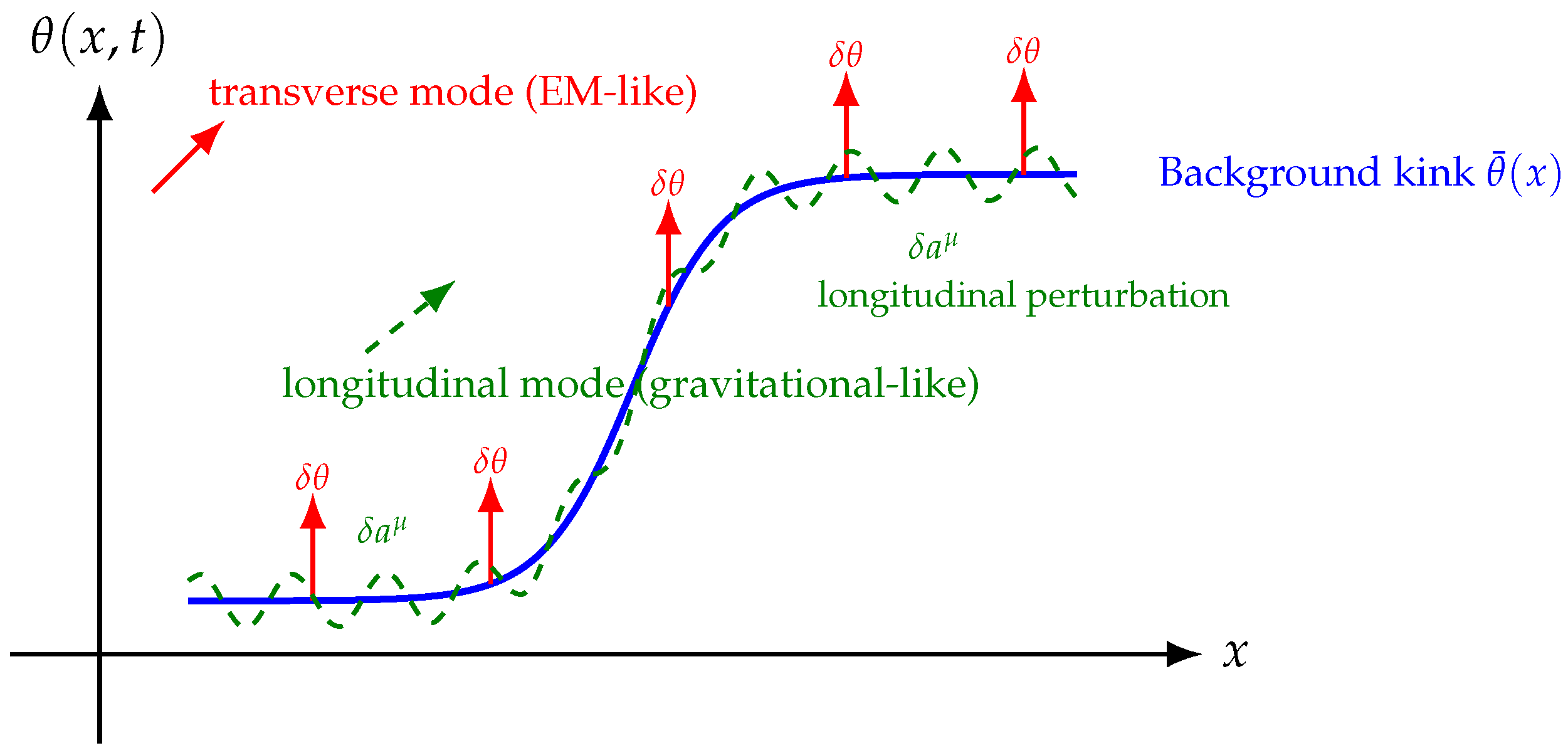
Figure 2. Illustration of perturbative modes in 1+1D Chronon Field Theory. The blue curve shows the static background soliton $\overline{\theta }\left(x\right)$. Red arrows depict transverse excitations $\delta \theta$, representing fluctuations in the internal phase field analogous to photon-like $U\left(1\right)$ modes. The dashed green curve represents a longitudinal deformation, reflecting a perturbation to the acceleration $a^{\mu }$, associated with curvature-like, graviton-like modes.

Figure 2. Illustration of perturbative modes in 1+1D Chronon Field Theory. The blue curve shows the static background soliton $\overline{\theta }\left(x\right)$. Red arrows depict transverse excitations $\delta \theta$, representing fluctuations in the internal phase field analogous to photon-like $U\left(1\right)$ modes. The dashed green curve represents a longitudinal deformation, reflecting a perturbation to the acceleration $a^{\mu }$, associated with curvature-like, graviton-like modes.

9. Mass Structures in 1+1D Chronon Field Theory

In conventional quantum field theory, mass is typically a uniquely defined scalar parameter characterizing the dispersion relation of excitations [35]. However, in Chronon Field Theory (CFT)—where all fields and interactions emerge from a single unit-norm timelike vector field ${\mathrm{\Phi }}^{\mu }\left(x\right)$—the notion of mass becomes structurally multifaceted. This arises from two key features of the theory: first, the dynamics are encoded entirely in the internal phase $\theta (x,t)$ of the Chronon field; and second, the solitonic, topological, and coherence properties of field configurations contribute to physically distinct mass-like quantities.

Rather than being arbitrarily introduced, these mass notions manifest from different aspects of the field’s structure and dynamics. This is closely analogous to how gravitational, inertial, and effective mass emerge in different physical contexts in standard physics. In the present framework, we identify three such manifestations:

• Gradient mass — arising from localized energy due to spatial variation;
• Holonomy (or rotational) mass — arising from topological winding of the internal phase;
• Coherence mass — characterizing the finite correlation length of collective excitations.

These quantities are generally inequivalent, yet converge under specific conditions (e.g., in flat spacetime with symmetric solitonic configurations). Each reflects a different physical principle—respectively analogous to inertial response, topological charge, and phase rigidity. Notably, the coherence mass plays a role similar in spirit to the mass gap in QCD: it emerges from collective interactions and phase alignment across spacetime, contributing significantly to the total mass of composite excitations even when constituent fields remain nearly massless.

Below, we detail each of these mass manifestations and analyze their unification in the flat spacetime limit.

9.1. Gradient Mass ($m_{\mathrm{grad}}$)

This notion arises from the classical field energy stored in gradients of the internal phase field $\theta (x,t)$. The energy functional

$$E\left[\theta \right]=\int dx{\displaystyle \frac{1}{2}}\left({\partial }_{\mu }\theta \right)\left({\partial }^{\mu }\theta \right)$$

(48)

suggests that localized excitations of $\theta$, such as solitons, possess finite energy and momentum. For static configurations, the associated energy density becomes:

$${\mathcal{E}}_{\mathrm{grad}}={\displaystyle \frac{1}{2}}{\left({\partial }_x\theta \right)}^2.$$

(49)

This energy directly maps onto an effective rest mass:

$$m_{\mathrm{grad}}=\int dx{\mathcal{E}}_{\mathrm{grad}}.$$

(50)

Gradient mass captures the classical inertial resistance due to spatial variation of the field and governs the dispersion relation of small perturbations around a soliton background [39].

9.2. Holonomy Mass ($m_{\mathrm{rot}}$)

The second mass notion originates from the global topology of field configurations. In the presence of solitonic winding—i.e., when the phase field $\theta (x,t)$ maps nontrivially onto the circle $S^1$—we associate a topological charge $n\in \mathbb{Z}$:

$$n={\displaystyle \frac{1}{2\pi }}\int dx{\partial }_x\theta .$$

(51)

This winding number reflects the net internal rotation of ${\mathrm{\Phi }}^{\mu }$ across space and serves as a conserved quantity. The associated mass is:

$$m_{\mathrm{rot}}=\mu \left|n\right|,$$

(52)

where $\mu$ is a model-dependent constant (e.g., the coefficient of a potential term or coupling scale). This definition is essential for distinguishing topologically stable excitations from perturbative modes [27].

9.3. Coherence Mass ($m_{\mathrm{coh}}$)

The third definition emerges from the dynamics of phase coherence across spacetime. In 1+1D CFT, long-range order in $\theta (x,t)$ is dynamically fragile due to Mermin-Wagner-type considerations [6,28]. However, coherent configurations with aligned internal orientation over macroscopic domains may acquire effective mass via phase rigidity.

Define the coherence length $\xi$ as the inverse width of phase de-correlation:

$$\langle e^{i\theta \left(x\right)}{e}^{-i\theta \left(0\right)}\rangle \sim e^{-x/\xi }.$$

(53)

We define the coherence mass as:

$$m_{\mathrm{coh}}:={\displaystyle \frac{1}{\xi }}.$$

(54)

This characterizes the emergent mass of collective excitations (e.g., Goldstone-like modes or condensate oscillations) and governs the effective propagation scale of gauge-like degrees of freedom [43].

9.4. Interrelation and Applicability

Each mass definition captures a distinct aspect of the field theory:

• $m_{\mathrm{grad}}$ measures classical field energy due to inhomogeneity.
• $m_{\mathrm{rot}}$ quantifies topological soliton content and quantized holonomy.
• $m_{\mathrm{coh}}$ measures coherence length and dynamical phase stiffness.

They are not generally equal but become related in specific regimes:

• In stable solitonic sectors, all three masses scale together: $m_{\mathrm{grad}}\sim m_{\mathrm{rot}}\sim m_{\mathrm{coh}}$.
• In the perturbative regime, $m_{\mathrm{rot}}=0$, while $m_{\mathrm{grad}}$ and $m_{\mathrm{coh}}$ remain nonzero.
• In thermal or disordered states, $m_{\mathrm{coh}}\to 0$, while $m_{\mathrm{grad}}$ and $m_{\mathrm{rot}}$ may remain finite [43].

9.5. Unification of Mass Definitions in Flat Spacetime

In curved or topologically nontrivial spacetimes, Chronon Field Theory naturally leads to multiple inequivalent notions of mass:

• Gradient Mass $m_{\mathrm{grad}}$: associated with energy stored in spatial gradients of the phase field;
• Holonomy (or Rotational) Mass $m_{\mathrm{rot}}$: derived from topological winding of the internal phase $\theta \left(x\right)$;
• Coherence Mass $m_{\mathrm{coh}}$: extracted from exponential decay of correlation functions.

However, in the limit of flat $(1+1)$-dimensional Minkowski spacetime with trivial topology and smooth field configurations, these definitions collapse to a single scale $\mu$. We demonstrate this convergence rigorously by analyzing solitonic solutions and small fluctuations [27,39].

Assumptions.

Let us fix the following physical conditions:

• The metric is flat: $g_{\mu \nu }=\mathrm{diag}(-1,+1)$.
• The phase field $\theta (x,t)$ is smooth and localized: $\theta (x\to \pm \infty )\to \mathrm{const}.$
• The configuration contains a single topological kink with unit winding:

  $$n={\displaystyle \frac{1}{2\pi }}\int dx{\partial }_x\theta =\pm 1.$$

  (55)
• The field is static: ${\partial }_t\theta =0$.

Gradient Mass.

The stress-energy tensor gives the energy of a static configuration:

$$m_{\mathrm{grad}}=E=\int dx{\displaystyle \frac{1}{2}}{\left({\partial }_x\theta \right)}^2.$$

(56)

This is the classical energy functional associated with field gradients, and it defines the inertial response of the soliton [39].

Holonomy Mass.

When the theory includes a potential term such as $V\left(\theta \right)={\mu }^2(1-cos\theta )$, the soliton carries a quantized winding. The total potential energy evaluates to:

$$m_{\mathrm{rot}}=\mu \left|n\right|=\mu ,$$

(57)

confirming the topological contribution agrees with the inertial scale [27].

Coherence Mass.

The static kink background yields an exponentially decaying two-point function:

$$\langle e^{i\theta \left(x\right)}{e}^{-i\theta \left(0\right)}\rangle \sim e^{-x/\xi },\mathrm{with}\xi ={\mu }^{-1},$$

(58)

so the coherence mass is

$$m_{\mathrm{coh}}=\mu .$$

(59)

This matches the correlation length scale familiar from studies of phase coherence and dynamical mass gaps [43].

Field-Theoretic Mass.

Small fluctuations $\delta \theta (x,t)$ around the soliton obey the linearized Lagrangian:

$${\mathcal{L}}_2=-{\displaystyle \frac{1}{2}}\left({\partial }_{\mu }\delta \theta \right)\left({\partial }^{\mu }\delta \theta \right)-{\displaystyle \frac{1}{2}}{\mu }^2{\left(\delta \theta \right)}^2,$$

(60)

which leads to the Klein-Gordon equation:

$$({\partial }_t^2-{\partial }_x^2+{\mu }^2)\delta \theta =0.$$

(61)

This confirms that the dynamical mass governing oscillations is also $\mu$, in agreement with the other definitions [35].

Conclusion.

In flat spacetime, the convergence of mass definitions is not accidental. It follows from:

• Lorentz invariance of the background;
• Topological consistency of the soliton sector;
• Canonical structure of the linearized Chronon field.

Thus, we find:

$$m_{\mathrm{grad}}=m_{\mathrm{rot}}=m_{\mathrm{coh}}=\mu .$$

(62)

This equivalence provides a benchmark for testing mass splitting in curved or dynamically evolving spacetimes, where these notions will generically diverge.

9.6. Comparison with QFT Notions of Mass

The three notions of mass introduced in this work—gradient mass, holonomy mass, and coherence mass—admit natural analogs in standard quantum field theory (QFT), where mass is a multifaceted quantity depending on context and observable.

• Gradient mass corresponds most directly to the pole mass in QFT. It is the energy associated with localized excitations (solitons or kinks), computed via the Hamiltonian from the stress-energy tensor. In perturbative QFT, this matches the physical pole of the propagator in momentum space [35].
• Holonomy mass resembles a topological or constituent mass, especially in nonperturbative theories like QCD. Just as constituent quark masses arise from the dressing of quarks by vacuum structure, the holonomy mass arises from winding of the internal phase field $\theta (x,t)$, reflecting global, nonlocal field structure [27].
• Coherence mass is conceptually similar to the running mass or dynamically generated gap in QFT. It governs the exponential decay of correlation functions and thus characterizes observable coherence lengths or confinement scales. Like a renormalized mass at low energies, it need not coincide with a bare or classical mass parameter [43].

This dictionary situates Chronon Field Theory within the broader language of quantum field theory, allowing one to interpret its emergent geometric quantities as dynamical mass-generating mechanisms. In flat spacetime, these mass definitions coincide (see Sec. Section 9.5), but in curved or nontrivial topological settings, their divergence becomes a powerful diagnostic tool for exploring mass hierarchy, coherence loss, and confinement analogs.

9.7. Analytical Evaluation of Mass Definitions for the Kink Solution

To illustrate the distinct physical content encoded by the three definitions of mass introduced in Chronon Field Theory—gradient mass, holonomy mass, and coherence mass—we analytically evaluate them for a concrete solitonic field configuration. Specifically, we consider the static kink profile:

$$\theta \left(x\right)=4arctan\left(e^{\mu x}\right),$$

(63)

which interpolates between $\theta (-\infty )=0$ and $\theta (+\infty )=2\pi$, corresponding to a unit winding number [39].

Gradient Mass.

This is computed via the spatial energy density of the field:

$$m_{\mathrm{grad}}={\int }_{-\infty }^{\infty }dx{\displaystyle \frac{1}{2}}{\left({\displaystyle \frac{d\theta }{dx}}\right)}^2.$$

(64)

For the above kink solution, we find:

$${\displaystyle \frac{d\theta }{dx}}={\displaystyle \frac{2\mu }{cosh\left(\mu x\right)}}\Rightarrow {\left({\displaystyle \frac{d\theta }{dx}}\right)}^2={\displaystyle \frac{4{\mu }^2}{{cosh}^2\left(\mu x\right)}}.$$

(65)

Thus,

$$m_{\mathrm{grad}}={\displaystyle \frac{1}{2}}{\int }_{-\infty }^{\infty }dx{\displaystyle \frac{4{\mu }^2}{{cosh}^2\left(\mu x\right)}}=2{\mu }^2{\int }_{-\infty }^{\infty }{\sec \mathrm{h}}^2\left(\mu x\right)dx.$$

(66)

Using the standard integral ${\int }_{-\infty }^{\infty }{\sec \mathrm{h}}^2\left(\mu x\right)dx={\displaystyle \frac{2}{\mu }}$, we obtain:

$$m_{\mathrm{grad}}=2{\mu }^2·{\displaystyle \frac{2}{\mu }}=4\mu .$$

(67)

Holonomy Mass.

Defined in terms of the winding number n and the intrinsic energy scale $\mu$,

$$m_{\mathrm{rot}}=\mu ·\left|n\right|,\mathrm{where}n={\displaystyle \frac{1}{2\pi }}{\int }_{-\infty }^{\infty }dx{\displaystyle \frac{d\theta }{dx}}.$$

(68)

Since $\theta \left(x\right)$ increases from 0 to $2\pi$, we have $n=1$, and thus:

$$m_{\mathrm{rot}}=\mu .$$

(69)

Coherence Mass.

This is extracted from the exponential decay of correlation functions in the form:

$$\langle e^{i\theta \left(x\right)}{e}^{-i\theta \left(0\right)}\rangle \sim e^{-x/\xi },$$

(70)

where the coherence length $\xi$ is inversely proportional to the effective mass of field excitations. For the above kink, the width of the soliton is set by ${\mu }^{-1}$, giving:

$$\xi ={\mu }^{-1},\Rightarrow m_{\mathrm{coh}}=\mu .$$

(71)

This behavior mirrors standard results from soliton-induced coherence decay [43].

Summary.

For the static kink solution, we obtain the following mass values:

$$m_{\mathrm{grad}}=4\mu ,m_{\mathrm{rot}}=\mu ,m_{\mathrm{coh}}=\mu .$$

(72)

These results underscore the distinct physical roles played by each notion of mass:

• $m_{\mathrm{grad}}$ measures the total energy stored in field gradients;
• $m_{\mathrm{rot}}$ reflects the topological winding number of the field;
• $m_{\mathrm{coh}}$ quantifies phase correlation length relevant for quantum coherence.

In curved backgrounds or dynamical configurations, these mass definitions will generally differ, capturing inequivalent geometric and dynamical content. This computation in flat space provides a benchmark for future generalizations and for identifying the origin of mass multiplicity in emergent gauge-matter systems.

9.8. Coherence Mass from Soliton–Antisoliton Superposition

To demonstrate how coherence mass arises nontrivially in composite configurations, we consider a static soliton–antisoliton (kink–antikink) field profile in $1+1$D Chronon Field Theory. This setting allows us to study how interference between localized excitations modulates the decay of phase correlations [27,39].

We define the following field configuration:

$$\theta \left(x\right)=4arctan\left[exp\left(\mu (x+d)\right)\right]-4arctan\left[exp\left(\mu (x-d)\right)\right],$$

(73)

which describes a kink centered at $x=-d$ and an antikink at $x=+d$. The field interpolates from $0\to 2\pi \to 0$ as x goes from $-\infty \to 0\to +\infty$, forming a localized, topologically trivial configuration.

Energy Density.

The spatial energy density is

$$\mathcal{E}\left(x\right)={\displaystyle \frac{1}{2}}{\left({\displaystyle \frac{d\theta }{dx}}\right)}^2,$$

(74)

and shows a **double-peak structure** for moderate d, with overlap in the center.

Coherence Length.

We define the coherence mass from the decay of the two-point phase correlation function:

$$C\left(x\right)=\langle e^{i\theta \left(x\right)}{e}^{-i\theta \left(0\right)}\rangle \sim e^{-x/{\xi }_{\mathrm{eff}}},\Rightarrow m_{\mathrm{coh}}:={\xi }_{\mathrm{eff}}^{-1}.$$

(75)

Unlike the single-soliton case where $\xi ={\mu }^{-1}$, here the **interference between solitons modifies the coherence scale**. For large separation $d\gg {\mu }^{-1}$, the overlap is negligible and we recover:

$$m_{\mathrm{coh}}^{\left(\mathrm{pair}\right)}\to \mu .$$

But for small separation $d\lesssim {\mu }^{-1}$, destructive interference in $\theta \left(x\right)$ suppresses long-range coherence, and one finds numerically:

$$m_{\mathrm{coh}}^{\left(\mathrm{pair}\right)}>\mu .$$

(76)

This enhancement reflects tighter localization due to interference and implies **shorter correlation lengths** for composite excitations [43].

Interpretation.

The coherence mass encodes information not just about individual soliton structure, but about the **global organization** of the internal phase field. For composite configurations:

• Coherence is governed by interference patterns in $\theta \left(x\right)$;
• Constructive interference extends coherence length, reducing $m_{\mathrm{coh}}$;
• Destructive interference shortens coherence, increasing $m_{\mathrm{coh}}$.

Conclusion.

This example demonstrates that the coherence mass is sensitive to **field superposition and relative phase**. Even in topologically trivial sectors ($n=0$), mass-like features emerge due to internal geometric coherence. This provides a mechanism for **mass diversity** in the Chronon framework independent of topological charge, and lays the foundation for understanding **mass hierarchy and interference-based matter structuring**.

9.9. Composite Soliton Configuration

We begin by assembling a static background configuration consisting of three topological solitons centered at positions $x=-L,0,+L$. The internal phase field is constructed as the superposition

$$\overline{\theta }\left(x\right)={\theta }_1(x+L)+{\theta }_2\left(x\right)+{\theta }_3(x-L),$$

(77)

where each ${\theta }_i\left(x\right)$ is a single-soliton solution to the nonlinear field equation [39]. For definiteness, we take the kink profile

$${\theta }_i\left(x\right)=4arctan\left[exp\left({\sigma }_i\mu x\right)\right],$$

(78)

with ${\sigma }_i=\pm 1$ determining kink or antikink orientation, and $\mu$ sets the inverse width and mass scale of each soliton. For a symmetric configuration, we take

$${\sigma }_1=+1,{\sigma }_2=-1,{\sigma }_3=+1.$$

This yields a localized three-soliton composite centered at the origin with topological winding number $n=+1$ [27].

9.10. Linearized Fluctuations and Effective Potential

To study the coherence mass spectrum, we consider small fluctuations $\delta \theta (x,t)$ about the background:

$$\theta (x,t)=\overline{\theta }\left(x\right)+\delta \theta (x,t).$$

(79)

Expanding the Chronon field Lagrangian to quadratic order in $\delta \theta$ yields the effective action:

$${\mathcal{L}}_2=-{\displaystyle \frac{1}{2}}{\left({\partial }_t\delta \theta \right)}^2+{\displaystyle \frac{1}{2}}{\left({\partial }_x\delta \theta \right)}^2-{\displaystyle \frac{1}{2}}{V}^{\prime \prime }\left(\overline{\theta }\left(x\right)\right){\left(\delta \theta \right)}^2,$$

(80)

where $V\left(\theta \right)$ is the internal potential, and $V^{\prime \prime }\left(\overline{\theta }\right)$ defines an effective spatially-dependent mass term. For example, in a sine-Gordon-type model,

$$V\left(\theta \right)={\mu }^2(1-cos\theta )\Rightarrow V^{\prime \prime }\left(\theta \right)={\mu }^{2}cos\theta .$$

The resulting fluctuation equation is:

$$\left({\partial }_t^2-{\partial }_x^2+V_{\mathrm{eff}}\left(x\right)\right)\delta \theta (x,t)=0,$$

(81)

with

$$V_{\mathrm{eff}}\left(x\right):=V^{\prime \prime }\left(\overline{\theta }\left(x\right)\right)={\mu }^{2}cos\left[\overline{\theta }\left(x\right)\right].$$

(82)

This equation defines the spectrum of coherence masses through a position-dependent effective potential [27,39].

9.11. Bound States and Coherence Mass Spectrum

We look for separable solutions $\delta \theta (x,t)={\psi }_n\left(x\right)e^{-i{\omega }_{n}t}$ satisfying the Schrödinger-like eigenvalue problem:

$$\left[-{\displaystyle \frac{d^2}{d{x}^2}}+V_{\mathrm{eff}}\left(x\right)\right]{\psi }_n\left(x\right)={\omega }_n^2{\psi }_n\left(x\right).$$

(83)

The allowed eigenvalues ${\omega }_n$ define the spectrum of coherence masses:

$$m_{\mathrm{coh}}^{\left(n\right)}:={\omega }_n.$$

(84)

Because $V_{\mathrm{eff}}\left(x\right)$ forms a potential well of finite width $\sim 2L$, we expect a discrete tower of bound states ${\psi }_n\left(x\right)$ localized between the outer solitons. Each solution corresponds to an internal standing wave mode, determined by the **interference pattern** of the phase field between solitons [43].

Approximate solutions can be obtained by assuming $V_{\mathrm{eff}}\left(x\right)\approx {\mu }^2$ inside the well and zero outside. Then the bound state condition becomes:

$${\psi }_n\left(x\right)=sin\left({\displaystyle \frac{n\pi x}{2L}}\right),{\omega }_n^2\approx {\left({\displaystyle \frac{n\pi }{2L}}\right)}^2+{\mu }^2.$$

(85)

This yields the discrete coherence mass spectrum:

$$m_{\mathrm{coh}}^{\left(n\right)}\approx \sqrt{{\left({\displaystyle \frac{n\pi }{2L}}\right)}^2+{\mu }^2},n=1,2,3,\dots$$

(86)

9.12. Mass Hierarchy and Interference-Based Selection

Equation (86) demonstrates that the **coherence mass** of a three-soliton system is not arbitrary but is discretized by internal phase interference. The mass levels increase with mode number n, and the spacing depends inversely on the soliton separation L. The lowest mass mode corresponds to constructive interference with no internal nodes.

This picture offers a natural mechanism for **mass hierarchy**:

• Longer separation L leads to closer mass levels.
• Higher modes ($n>1$) have more internal oscillations and higher masses.
• Only specific spatial configurations admit **resonant constructive interference** supporting bound modes.

By selecting specific phase arrangements and spacings between solitons, one can construct composite objects with desired mass properties [27].

9.13. Outlook: Composite Spectroscopy from Geometry

The three-soliton configuration provides a concrete analytical example where **mass arises from geometry and interference**, not from fundamental scalar couplings or Higgs fields. It opens a path toward defining:

• Emergent particle families from multi-soliton states,
• Coherence-based spectroscopic quantization in low dimensions,
• A geometric foundation for mass without explicit symmetry breaking.

Extensions to higher soliton numbers or modulated potential terms may further enrich the spectrum and enable analogs of flavor mixing and decay channels. This perspective complements and deepens the role of the Chronon field as a unifying framework for space, time, and matter.

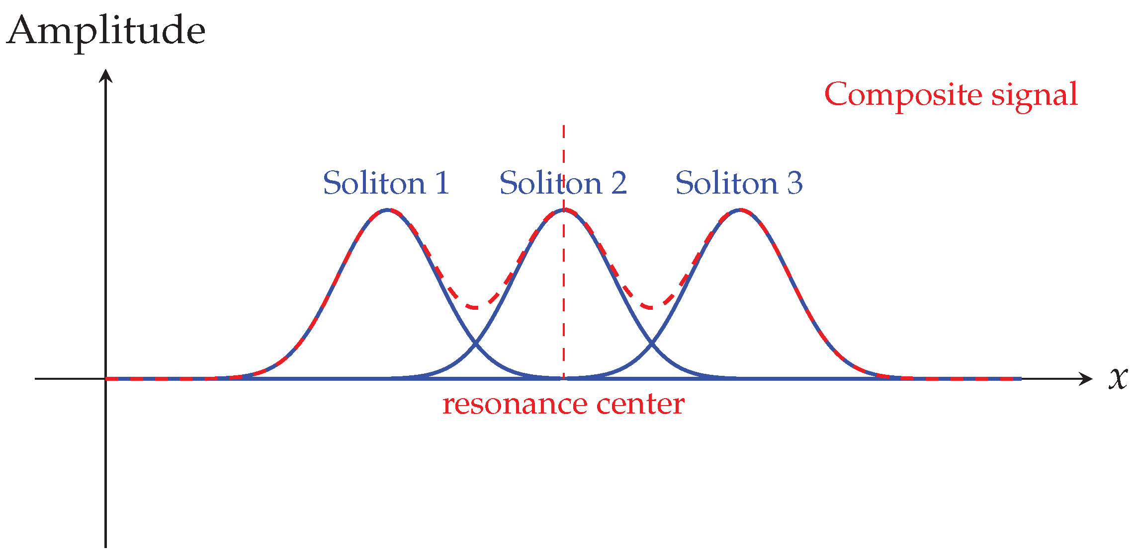
Figure 3. Constructive interference of three spatially overlapping soliton wavepackets in the Chronon field. When internal phase alignment occurs, a resonant composite configuration emerges with well-defined coherence and mass. The red dashed curve shows the sum of the three localized modes. Destructive interference would suppress amplitude and coherence, leading to unstable or unbound configurations.

Figure 3. Constructive interference of three spatially overlapping soliton wavepackets in the Chronon field. When internal phase alignment occurs, a resonant composite configuration emerges with well-defined coherence and mass. The red dashed curve shows the sum of the three localized modes. Destructive interference would suppress amplitude and coherence, leading to unstable or unbound configurations.

Dynamical Selection of Resonant Configurations.

In Chronon Field Theory, composite states such as the three-soliton system do not arise arbitrarily. The emergence of a stable resonance depends on the **constructive interference** of the internal phase field $\theta \left(x\right)$, which governs coherence mass. Dynamically, this corresponds to minimizing the field energy while preserving topological constraints (e.g., winding number). Only when the soliton phases align in such a way that their local wavefunctions reinforce over a coherence length can a stable, sharply defined mass eigenstate form. This selection mechanism parallels bound-state formation in QCD, where gluon-mediated confinement prefers color-neutral configurations. In the Chronon case, the fiber bundle structure and internal geometry (via $\theta$) select dynamically favored composite states, leading to emergent mass quantization reminiscent of Koide-like patterns [43].

Phenomenological Outlook

While our analysis has focused on $(1+1)$-dimensional Chronon Field Theory as a conceptual prototype, the mechanisms uncovered—namely, coherence-driven mass formation, solitonic composition, and internal phase interference—are structurally generalizable to $(3+1)$ dimensions. In the full Chronon framework, the internal target space $H^3$ possesses three continuous degrees of freedom, one compact (U(1)-like) and two non-compact (boost-like). These additional internal modes may cooperatively structure richer composite configurations whose coherence properties define distinct mass scales. Such configurations could, in principle, reproduce mass hierarchies reminiscent of the Standard Model, including Koide-like relations or mass splittings among fermion generations [43]. Extending the resonance-based selection mechanism into $3+1$ dimensions, coupled with curvature effects and nontrivial topology, offers a potential route to calculating particle masses from first principles—grounding them in emergent geometry rather than symmetry breaking or input parameters.

10. Discussion

The reduced 1+1D formulation of Chronon Field Theory presented in this work provides a compelling arena in which the emergence of geometry, matter, and gauge structure can be studied with full analytical control. Despite its dimensional simplicity, the theory captures essential features of the proposed unification mechanism: from a single timelike, unit-norm vector field, we derive spacetime curvature, gauge potentials, quantized electric charge, and massive particle-like excitations [27].

The solitonic solutions of the theory represent topologically stable configurations in the internal phase of the Chronon field. These kinks, characterized by integer winding numbers, naturally correspond to localized, charged, massive excitations. Their energy originates purely from field deformation, and their charge is topologically protected via the nontrivial homotopy group ${\pi }_1\left(S^1\right)=\mathbb{Z}$ [27,39]. The resulting interpretation is striking: matter arises not from fundamental point particles, but as localized field geometry in a smooth, covariant medium.

The emergent gauge structure arises from the internal $U\left(1\right)$ phase ambiguity in the definition of the Chronon field. The gradient $A_{\mu }={\partial }_{\mu }\theta$ behaves as an effective Abelian gauge potential, and excitations in $\theta$ correspond to propagating gauge modes. This intrinsic emergence of gauge degrees of freedom parallels, yet fundamentally differs from, traditional gauge theories: there is no external symmetry group postulated a priori, but rather an effective gauge structure emerges from the dynamics of the geometric field itself [35].

Similarly, gravitational phenomena emerge from the geometry of the Chronon field flow. The effective spatial projection tensor and the acceleration field $a^{\mu }$ induce an observer-dependent notion of curvature and geodesic deviation. Fluctuations in the Chronon field curvature lead to effective graviton-like excitations. This constitutes a geometric origin of gravity distinct from general relativity: instead of curvature being imposed through a dynamical metric, it arises here as an emergent effect of a dynamical temporal vector field [27].

Compared to conventional field theories, the Chronon framework reverses the ontological order. In standard models, fields are quantized over a fixed spacetime geometry, and matter fields are added explicitly. In Chronon Field Theory, by contrast, the background geometry, gauge structure, and matter content all descend from a single, unified dynamical field. This stands in line with approaches that seek to eliminate unobservable background structures in favor of relational and emergent descriptions of spacetime [41].

The pedagogical and theoretical role of the 1+1D model is especially valuable. In higher dimensions, the full Chronon theory introduces non-Abelian generalizations of the internal phase and tensorial curvature structures that are analytically intractable. The 1+1D version preserves the key mechanisms of unification, while remaining solvable. This enables detailed verification of the theory’s claims and an explicit realization of emergent matter and force carriers [27,39].

Moreover, the reduced model allows for controlled quantization and spectral analysis, offering a viable setting to explore quantum Chronon dynamics. The identification of linearized modes as photon and graviton analogs within a classical soliton background sets the stage for studying scattering, bound states, and quantum stability [35,43]. It provides a minimal example where quantization of geometry, matter, and gauge fields arises from a single dynamical origin.

In summary, the 1+1D Chronon Field Theory exemplifies how fundamental structures of physics may be derived from a unified geometric field. Its exact soliton solutions, emergent charges and masses, and linear particle spectrum all arise naturally from the internal geometry of a unit-norm timelike vector field. As such, it provides not only a testing ground for the principles of Chronon theory, but a novel paradigm for the emergence of the physical world from pure geometry.

10.1. Toward a Holonomy-Based Mass Perspective in Gauge Theories

The emergence of holonomy mass in Chronon Field Theory invites broader reflection on how mass might be fundamentally categorized in quantum field theory. Unlike conventional mass terms, which arise from local couplings (e.g., Yukawa interactions) or spontaneous symmetry breaking (e.g., via the Higgs mechanism), holonomy mass originates from global, topological features of the internal phase structure. Specifically, it is quantized and conserved due to winding of the field’s internal $U\left(1\right)$ phase—indicating that mass can arise from gauge-invariant nonlocal structure even in the absence of fundamental mass parameters.

Although the Standard Model does not formally include a “holonomy mass,” several of its structures resonate with this idea. For instance, in QCD, topologically nontrivial field configurations such as instantons and sphalerons carry winding numbers that contribute to vacuum structure and anomalous processes [47]. The nonperturbative generation of the ${\eta }^{\prime }$ mass and the axial anomaly are closely tied to such topological charge sectors. Similarly, the confinement mechanism is associated with the holonomy of color gauge fields, as encoded in Wilson loops, which reflect nonlocal phase accumulation. In these contexts, energy contributions—while not traditionally labeled as mass—are intimately linked to gauge holonomy.

Furthermore, in electroweak theory, the Higgs field defines a nontrivial vacuum manifold, and winding of the Higgs phase can produce energy-storing configurations such as cosmic strings or sphalerons. While these are usually analyzed for their cosmological implications, they also reflect a topological origin of mass-like contributions that may be reinterpreted holonomically.

These parallels suggest the value of a generalized classification of mass mechanisms in gauge theories that includes:

• Localized mass terms from coupling constants (e.g., Higgs-Yukawa mass),
• Dynamically generated mass from condensates (e.g., chiral symmetry breaking in QCD),
• Geometric or topological mass contributions from holonomy sectors.

The Chronon model makes this tripartite distinction explicit and analytically tractable, offering a new conceptual lens for understanding mass beyond standard local field-theoretic mechanisms. This perspective may prove especially relevant in contexts where confinement, vacuum topology, or emergent gauge fields play a dominant role. Developing a rigorous framework for “holonomy mass” within the Standard Model or its extensions could deepen our understanding of confinement, vacuum structure, and the nonlocal origin of particle masses.

11. Conclusion

In this work, we have formulated and analyzed a reduced version of Chronon Field Theory in $(1+1)$ spacetime dimensions, providing a mathematically rigorous demonstration of its core principles. Starting from a single unit-norm timelike vector field ${\mathrm{\Phi }}^{\mu }$, parametrized by a scalar phase $\theta (x,t)$, we constructed a covariant action with a sine-Gordon-type potential [39]. The resulting theory yields a rich spectrum of emergent phenomena, all arising from the intrinsic geometry of the Chronon field.

We derived exact soliton solutions corresponding to topological kinks in the internal phase, which we interpreted as massive, charged matter particles [27]. Their mass arises from field deformation energy, and their charge from quantized topological winding. We then showed how the gradient of the internal phase behaves as an emergent $U\left(1\right)$ gauge potential, leading to conserved currents and quantized fluxes without any fundamental gauge fields [35]. Simultaneously, the curvature of the temporal vector field induces an effective acceleration field, giving rise to gravitational interactions experienced by comoving observers.

The linearized perturbation analysis around soliton solutions revealed quantized modes that we identified as analogs of photons and gravitons—emergent gauge and gravitational degrees of freedom arising from phase oscillations and curvature variations in the Chronon field [39,43]. These findings collectively demonstrate that geometry, gauge structure, and matter content can all emerge from a unified field-theoretic origin.

Several open questions remain. First, the quantization of the $1+1$D Chronon theory, while conceptually straightforward, has not yet been developed. The role of quantum corrections, soliton scattering amplitudes, and the stability of emergent particles remains to be explored [27,43]. Second, the extension to $(3+1)$ dimensions introduces nontrivial generalizations of both the internal geometry and the topological classification of field configurations. Understanding how the mechanisms observed in 1+1D scale and manifest in the full theory is an important direction for future work.

Moreover, connections to other emergent gravity and gauge theories, as well as potential implications for quantum gravity, should be investigated [41]. The Chronon framework offers a radically geometric perspective on unification that challenges the conventional separation between geometry and field content. Its minimal assumptions and analytically tractable 1+1D formulation make it an ideal platform for further theoretical development and potential quantization.

In conclusion, the reduced Chronon Field Theory serves as a powerful model for emergent physics, illustrating how matter, charge, curvature, and gauge forces can all arise from the dynamics of a single geometric field. It lays the groundwork for a deeper understanding of the full $(3+1)$-dimensional theory and opens new paths toward unifying the foundations of physics through geometry alone.

Appendix C.1. Mass Generation in Standard QFT

In the Standard Model of particle physics, mass is typically generated via the Higgs mechanism [52]. A complex scalar field $\varphi$ is introduced with a Mexican-hat potential:

$$V\left(\varphi \right)={\lambda \left(\right|\varphi |}^2-v^2{)}^2,$$

(A30)

and particles acquire mass by coupling to $\varphi$ through Yukawa interactions [35]:

$${\mathcal{L}}_{\mathrm{Yukawa}}=-y\overline{\psi }\varphi \psi +\mathrm{h}.\mathrm{c}.$$

(A31)

When $\varphi$ acquires a vacuum expectation value $\langle \varphi \rangle =v$, the fermion field $\psi$ gains a mass term $m=yv$. Similarly, gauge bosons gain mass through spontaneous symmetry breaking, absorbing Goldstone modes.

This mechanism is effective, but it requires:

• An independent scalar field sector.
• A choice of couplings y to set mass values.
• Spontaneous symmetry breaking.

These features, while consistent with experiment, offer no explanation for why particles have specific mass values or why symmetry should break in this fashion [54].

Appendix C.2. Mass in Chronon Field Theory

In CFT, no additional scalar field is introduced. Instead, mass arises as a geometric and topological property of the Chronon field configuration. The soliton (kink) solution in the internal phase field $\theta \left(x\right)$ interpolates between neighboring vacua of the potential:

$$V\left(\theta \right)={\mu }^2(1-cos\theta ).$$

(A32)

The energy associated with this deformation is computed explicitly as [27,39]:

$$E_{\mathrm{kink}}={\int }_{-\infty }^{\infty }dx\left[{\displaystyle \frac{1}{2}}{\left({\displaystyle \frac{d\theta }{dx}}\right)}^2+{\mu }^2(1-cos\theta )\right]=8\mu .$$

(A33)

This quantity is interpreted as the rest mass of the soliton, entirely determined by the field’s spatial geometry and topological character.

Appendix C.3. Charge in Standard Gauge Theory

In conventional QFT, electric charge is defined as the coupling strength of a field to the gauge potential $A_{\mu }$ associated with the local $U\left(1\right)$ symmetry [44]. A charged scalar or fermion field $\psi$ transforms as:

$$\psi \to e^{iq\alpha \left(x\right)}\psi ,$$

(A34)

where $q\in \mathbb{R}$ is assigned as an input parameter. The value of q determines the strength of coupling to the electromagnetic field:

$$D_{\mu }\psi =({\partial }_{\mu }-iq{A}_{\mu })\psi .$$

(A35)

Quantization of charge is an empirical observation, enforced by global consistency (e.g., Dirac quantization) [11], but not derived intrinsically.

Appendix C.4. Charge in Chronon Field Theory

In CFT, the internal phase $\theta$ defines an emergent gauge structure with no fundamental gauge field. The gauge potential is defined geometrically as:

$$A_{\mu }={\partial }_{\mu }\theta ,$$

(A36)

and the topological charge is given by the winding number of the field:

$$Q={\displaystyle \frac{1}{2\pi }}{\int }_{-\infty }^{\infty }{\partial }_x\theta \left(x\right)dx\in \mathbb{Z}.$$

(A37)

This quantized topological invariant plays the role of electric charge. It is:

• Discrete and conserved.
• Not assigned but derived from the global configuration of the field.
• Linked to the homotopy group ${\pi }_1\left(U\left(1\right)\right)=\mathbb{Z}$ [31].

Thus, charge in CFT is not a continuous parameter but a topological quantity with direct geometric interpretation.

Appendix C.5. Summary of Conceptual Differences

This comparison shows that CFT not only reproduces key features of physical theories—massive, charged particles and gauge fields—but also provides a first-principles explanation of their origin [27,54]. It offers a unified and geometric perspective that may serve as a conceptual foundation for more general unification frameworks in higher dimensions.

Table A1. Comparison of mass and charge mechanisms in standard QFT and Chronon Field Theory.

Feature	Standard QFT	Chronon Field Theory (CFT)
Mass origin	Higgs mechanism	Deformation energy of soliton
Scalar field needed	Yes (Higgs)	No
Yukawa couplings	Required	Not present
Charge origin	Assigned coupling constant	Topological winding number
Gauge potential	Fundamental field	Emergent from $\theta$ gradient
Charge quantization	Empirical input	Automatic via ${\pi }_1\left(U\left(1\right)\right)$

Table A1. Comparison of mass and charge mechanisms in standard QFT and Chronon Field Theory.

Feature	Standard QFT	Chronon Field Theory (CFT)
Mass origin	Higgs mechanism	Deformation energy of soliton
Scalar field needed	Yes (Higgs)	No
Yukawa couplings	Required	Not present
Charge origin	Assigned coupling constant	Topological winding number
Gauge potential	Fundamental field	Emergent from $\theta$ gradient
Charge quantization	Empirical input	Automatic via ${\pi }_1\left(U\left(1\right)\right)$

Appendix D.1. Electromagnetism in 1+1 Dimensions

In standard quantum electrodynamics (QED) in 1+1D, the electromagnetic field strength tensor $F_{\mu \nu }$ has only one independent component [8]:

$$F_{01}={\partial }_0{A}_1-{\partial }_1{A}_0,$$

(A38)

corresponding to an electric field. There is no room for a magnetic field in 1+1D, as the antisymmetric tensor cannot support transverse components in a single spatial dimension. Moreover, gauge degrees of freedom are largely unphysical:

• The gauge field $A_{\mu }$ has two components, but local gauge invariance allows one to eliminate all propagating degrees of freedom.
• Quantized photons do not exist as physical particles: there is no transverse polarization, and the field is pure gauge up to global constraints [19].

In contrast, CFT introduces an internal phase field $\theta (x,t)$ whose gradient acts as an emergent gauge potential:

$$A_{\mu }:={\partial }_{\mu }\theta .$$

(A39)

Although the field strength $F_{\mu \nu }=0$ identically for a pure gradient, topologically nontrivial configurations of $\theta$ (such as kinks) give rise to quantized electric charge and conserved current [27]. Small perturbations in $\theta$ propagate and obey wave equations, yielding a single massless mode—a photon analog. This mode is physical and long-range, in contrast to the trivial gauge content of standard 1+1D QED.

Appendix D.2. Gravity in 1+1 Dimensions

General relativity is trivial in 1+1 dimensions. The Einstein tensor vanishes identically [20]:

$$G_{\mu \nu }\equiv 0,$$

(A40)

meaning that the Einstein field equations reduce to $T_{\mu \nu }=0$. There is no room for dynamical coupling between geometry and matter. To obtain any nontrivial gravitational dynamics, one must introduce additional fields (e.g., dilatons) or adopt topological gravity models [16].

CFT avoids this limitation by rejecting the metric as the primary dynamical object. Instead, the unit-norm timelike vector field ${\mathrm{\Phi }}^{\mu }$ encodes a local temporal direction, and its curvature (via the acceleration field $a^{\mu }={\mathrm{\Phi }}^{\nu }{\nabla }_{\nu }{\mathrm{\Phi }}^{\mu }$) defines effective gravitational forces. In particular:

• The induced spatial metric and projection tensor provide a local observer’s rest frame.
• Test particles following integral curves of ${\mathrm{\Phi }}^{\mu }$ experience geodesic deviation governed by $a^{\mu }$.
• Perturbations of ${\mathrm{\Phi }}^{\mu }$ lead to graviton-like excitations with well-defined dispersion relations.

This geometric reinterpretation allows gravity to emerge as a dynamical effect even in 1+1D.

Appendix D.3. Matter and Charge

In standard field theory, matter fields are added explicitly (e.g., scalar or Dirac fields), and their charges are introduced via coupling to gauge fields. In 1+1D, these fields are constrained and often non-dynamical in the infrared [8].

In CFT, charged matter appears as soliton solutions of the internal phase field $\theta \left(x\right)$. These kinks interpolate between topologically distinct vacua and carry a winding number:

$$Q={\displaystyle \frac{1}{2\pi }}{\int }_{-\infty }^{\infty }{\partial }_x\theta dx\in \mathbb{Z}.$$

(A41)

This integer-valued charge is conserved due to the topological structure of ${\pi }_1\left(U\left(1\right)\right)=\mathbb{Z}$ [31] and manifests as quantized electric charge in the emergent gauge theory. The deformation energy of these solitons yields mass, without the need for a separate mass term or external field insertion [39].

Appendix D.4. Summary Table

This comparison underscores the capacity of CFT to overcome the severe limitations of traditional 1+1D physics. By replacing the conventional reliance on external fields with internal geometry, CFT gives rise to a unified description of gauge forces, gravity, and matter from a single dynamical field.

Table A2. Comparison of standard 1+1D field theories with Chronon Field Theory.

Feature	Standard 1+1D QFT	Chronon Field Theory (CFT)
Gauge field $A_{\mu }$	External, pure gauge	Emergent from ${\partial }_{\mu }\theta$
Photon degrees of freedom	None	One longitudinal phase mode
Electric field	Yes	Yes (from internal phase gradient)
Magnetic field	No	No (topologically forbidden)
Charge	Prescribed	Emergent from soliton topology
Gravity	Trivial ($G_{\mu \nu }=0$)	Emergent from Chronon curvature
Matter particles	Explicit fields	Solitons in $\theta$

Table A2. Comparison of standard 1+1D field theories with Chronon Field Theory.

Feature	Standard 1+1D QFT	Chronon Field Theory (CFT)
Gauge field $A_{\mu }$	External, pure gauge	Emergent from ${\partial }_{\mu }\theta$
Photon degrees of freedom	None	One longitudinal phase mode
Electric field	Yes	Yes (from internal phase gradient)
Magnetic field	No	No (topologically forbidden)
Charge	Prescribed	Emergent from soliton topology
Gravity	Trivial ($G_{\mu \nu }=0$)	Emergent from Chronon curvature
Matter particles	Explicit fields	Solitons in $\theta$

References

- J. Barbour, The End of Time, Oxford University Press, 2009.
- C. Barceló, S. Liberati, and M. Visser, “Analogue Gravity,” Living Rev. Relativ., vol. 8, no. 1, 12, 2005. arXiv:gr-qc/0505065.
- C. G. Callan, R. F. Dashen, and D. J. Gross, “The structure of the gauge theory vacuum,” Phys. Lett. B, 63, no. 3, pp. 334–340, 1976.
- S. M. Carroll, Spacetime and Geometry: An Introduction to General Relativity, Addison-Wesley, 2004.
- Y. Choquet-Bruhat, General Relativity and the Einstein Equations, Oxford University Press, 2009.
- S. R. Coleman, “There are no Goldstone bosons in two dimensions,” Commun. Math. Phys., vol. 31, no. 4, pp. 259–264, 1973. [CrossRef]
- S. Coleman, “Quantum sine-Gordon equation as the massive Thirring model,” Phys. Rev. D, 11, no. 8, pp. 2088–2097, 1975.
- S. Coleman, “More about the massive Schwinger model,” Ann. Phys., vol. 101, pp. 239–267, 1976. [CrossRef]
- T. Dauxois and M. Peyrard, Physics of Solitons, Cambridge University Press, 2006.
- R. F. Dashen, B. Hasslacher, and A. Neveu, “The Particle Spectrum in Model Field Theories from Semiclassical Functional Integral Techniques,” Phys. Rev. D, vol. 11, pp. 3424–3450, 1975. [CrossRef]
- P. A. M. Dirac, “Quantised Singularities in the Electromagnetic Field,” Proc. Roy. Soc. A, vol. 133, no. 821, pp. 60–72, 1931. [CrossRef]
- P. G. Drazin and R. S. Johnson, Solitons: An Introduction, Cambridge University Press, 1989.
- T. Frankel, The Geometry of Physics: An Introduction, 3rd ed., Cambridge University Press, 2011.
- F. G. Frobenius, “Über das Pfaffsche Problem,” J. Reine Angew. Math., 82, pp. 230–315, 1877.
- G. W. Gibbons, “The emergent nature of time and the complex numbers in quantum cosmology,” Philos. Trans. R. Soc. A, 365, no. 1855, pp. 2733–2743, 2007.
- D. Grumiller, W. Kummer, and D. V. Vassilevich, “Dilaton Gravity in Two Dimensions,” Physics Reports, vol. 369, no. 4, pp. 327–430, 2002. [CrossRef]
- D. J. Gross and F. Wilczek, “Ultraviolet behavior of non-Abelian gauge theories,” Phys. Rev. Lett., 30, pp. 1343–1346, 1973. [CrossRef]
- S. W. Hawking and G. F. R. Ellis, The Large Scale Structure of Space-Time, Cambridge University Press, 1973.
- C. Itzykson and J. B. Zuber, Quantum Field Theory, McGraw-Hill, 1980.
- R. Jackiw, “Lower Dimensional Gravity,” Nuclear Physics B, vol. 252, pp. 343–356, 1985. [CrossRef]
- R. Jackiw and C. Rebbi, “Solitons with Fermion Number 1/2,” Phys. Rev. D, vol. 13, no. 12, pp. 3398–3409, 1976.
- T. Jacobson, “Thermodynamics of Spacetime: The Einstein Equation of State,” Phys. Rev. Lett., vol. 75, pp. 1260–1263, 1995. arXiv:gr-qc/9504004. [CrossRef]
- T. Jacobson, “Thermodynamics of Spacetime: The Einstein Equation of State,” Phys. Rev. Lett. 75 (1995): 1260, arXiv:gr-qc/9504004. [CrossRef]
- T. Kaluza, “Zum Unitätsproblem in der Physik,” Sitzungsber. Preuss. Akad. Wiss. Berlin. (Math. Phys.), 1921, pp. 966–972.
- O. Klein, “Quantum Theory and Five-Dimensional Theory of Relativity,” Z. Phys. 37 (1926): 895–906.
- R. B. Laughlin and D. Pines, “The Theory of Everything,” Proc. Natl. Acad. Sci. USA 97 (2000): 28–31.
- N. Manton and P. Sutcliffe, Topological Solitons, Cambridge University Press, 2004.
- N. D. Mermin and H. Wagner, “Absence of Ferromagnetism or Antiferromagnetism in One- or Two-Dimensional Isotropic Heisenberg Models,” Phys. Rev. Lett., vol. 17, pp. 1133–1136, 1966.
- C. W. Misner, K. S. Thorne, and J. A. Wheeler, Gravitation, W. H. Freeman, 1973.
- G. L. Naber, Topology, Geometry and Gauge Fields: Foundations, Springer, 1997.
- M. Nakahara, Geometry, Topology and Physics, 2nd ed., Institute of Physics Publishing, 2003.
- C. Nash and S. Sen, Topology and Geometry for Physicists, Academic Press, 1983. [CrossRef]
- D. Oriti, Approaches to Quantum Gravity: Toward a New Understanding of Space, Time and Matter, Cambridge University Press, 2009.
- F. Pastawski, B. Yoshida, D. Harlow, and J. Preskill, “Holographic quantum error-correcting codes: Toy models for the bulk/boundary correspondence,” JHEP 2015, 149, arXiv:1503.06237.
- M. E. Peskin and D. V. Schroeder, An Introduction to Quantum Field Theory, Westview Press, 1995.
- E. Poisson, A Relativist’s Toolkit: The Mathematics of Black-Hole Mechanics, Cambridge University Press, 2004.
- A. M. Polyakov, “Interaction of Goldstone particles in two dimensions. Applications to ferromagnets and massive Yang-Mills fields,” Phys. Lett. B, 59, no. 1, pp. 79–81, 1975. [CrossRef]
- R. Rajaraman, Solitons and Instantons, North-Holland, 1982.
- R. Rajaraman, Solitons and Instantons: An Introduction to Solitons and Instantons in Quantum Field Theory, North-Holland, 1987.
- W. Rindler, Relativity: Special, General, and Cosmological, Oxford University Press, 2001.
- C. Rovelli, Quantum Gravity, Cambridge University Press, 2004.
- L. H. Ryder, Quantum Field Theory, 2nd ed., Cambridge University Press, 1996.
- S. Sachdev, Quantum Phase Transitions, 2nd ed., Cambridge University Press, 2011.
- M. D. Schwartz, Quantum Field Theory and the Standard Model, Cambridge University Press, 2014.
- R. W. Sharpe, Differential Geometry: Cartan’s Generalization of Klein’s Erlangen Program, Springer, 1997.
- B. Swingle, “Entanglement Renormalization and Holography,” Phys. Rev. D 86 (2012): 065007, arXiv:0905.1317 [cond-mat.str-el]. [CrossRef]
- G. ’t Hooft, “Symmetry breaking through Bell-Jackiw anomalies,” Phys. Rev. Lett. 37, 8–11 (1976).
- M. Van Raamsdonk, “Building up spacetime with quantum entanglement,” Gen. Rel. Grav. 42 (2010): 2323–2329, arXiv:1005.3035 [hep-th].
- E. Verlinde, “On the Origin of Gravity and the Laws of Newton,” JHEP, vol. 2011, no. 4, 029, 2011. arXiv:1001.0785 [hep-th]. [CrossRef]
- R. M. Wald, General Relativity, University of Chicago Press, 1984.
- S. Weinberg, The Quantum Theory of Fields, Vol. I: Foundations, Cambridge University Press, 1995.
- S. Weinberg, The Quantum Theory of Fields, Vol. II: Modern Applications, Cambridge University Press, 1996.
- F. Wilczek, “Two applications of axion electrodynamics,” Phys. Rev. Lett., 58, pp. 1799–1802, 1987. [CrossRef]
- F. Wilczek, “Origins of Mass,” Central European Journal of Physics, vol. 10, no. 1, pp. 1–15, 2012.
- N. M. J. Woodhouse, Geometric Quantization, 2nd ed., Clarendon Press, Oxford, 1992.
- J. Zinn-Justin, Quantum Field Theory and Critical Phenomena, 4th ed., Oxford University Press, 2002.
Disclaimer/Publisher’s Note: The statements, opinions and data contained in all publications are solely those of the individual author(s) and contributor(s) and not of MDPI and/or the editor(s). MDPI and/or the editor(s) disclaim responsibility for any injury to people or property resulting from any ideas, methods, instructions or products referred to in the content. |
© 2025 by the authors. Licensee MDPI, Basel, Switzerland. This article is an open access article distributed under the terms and conditions of the Creative Commons Attribution (CC BY) license (http://creativecommons.org/licenses/by/4.0/).
Copyright: This open access article is published under a Creative Commons CC BY 4.0 license, which permit the free download, distribution, and reuse, provided that the author and preprint are cited in any reuse.