Submitted:
01 August 2025
Posted:
01 August 2025
You are already at the latest version
Abstract
This work presents the active control of nonlinear vibrations of a piezoelectric-elastic-piezoelectric sandwich beam, subjected to transverse excitation while neglecting axial displacement effects. By using a structure with piezoelectric actuators and sensors, and taking into account geometric nonlinearities, a nonlinear vibration control model was obtained through a feedback control law. The dynamic equation of the structure is derived by applying the variational principle and Hamilton’s principle. This equation is solved under primary and secondary resonance by adopting the method of averaging as a perturbation scheme and Galerkin’s approximation. The simulation results of amplitude-frequency responses are presented and discussed for different values of control gains and for three boundary conditions. Our results are in good agreement with those obtained by other methods.
Keywords:
piezoelectric
; sandwich beam
; nonlinear vibrations
; active control
; method of averaging
1. Introduction
Structural vibrations are highly undesirable, as they can lead to issues such as structural fatigue, transmission of vibrations to other systems, and external or internal noise due to acoustic radiation, among others [1,2,3]. In many industrial and defense applications, noise and vibrations represent a major challenge. Conventional mitigation methods, which rely on passive damping techniques, often prove ineffective at low frequencies. In this context, active control methods appear to be more suitable [4,5,6,7,8,9]. The principle of these so-called active techniques is to generate a field that interferes with the disturbance field. The superimposed field must therefore match the disturbance in amplitude but be opposite in phase for each relevant frequency. While the principle is straightforward, its implementation is much more complex, as the disturbance is often unpredictable and composed of multiple frequencies. Moreover, disturbance minimization is often required over a wide spatial domain, further complicating the problem [10].
Although active control was conceived in the 1930s, it only truly advanced with the emergence of digital signal processors in the 1980s. While some applications of this technology have already been developed, many are still under research, particularly in the aerospace, avionics, and automotive sectors. Focusing specifically on active vibration control, advancements remain relatively recent. In fact, the additional size and mass introduced by the sensors and actuators required for active vibration control have long hindered the development of many applications. Only in the last few decades has the use of piezoelectric material-based transducers enabled significant progress. Due to their compactness, low weight, and electro-mechanical conversion capabilities, piezoelectric materials exhibit all the necessary qualities for use in active vibration control systems. Moreover, they can serve both as electromechanical actuators and vibration sensors in the system [11,12].
To reduce stresses in materials, extend their service life, enhance structural safety (e.g., in transportation), and improve user comfort, the control and damping of mechanical vibrations has been the subject of extensive scientific research over many decades. Furthermore, the recent proliferation of so-called “smart materials” which couple multiple physical fields such as mechanics and electricity has led to the development of reliable, robust, and efficient vibration control techniques that are also highly integrable. These techniques are therefore well-suited for embedded systems or structures with strict space constraints [11]. In this regard, Rechdaoui et al. [12,13,14] developed an active control method for nonlinear vibrations of a piezoelectric–elastic sandwich beam based on the method of multiple scales. Similarly, Belouettar et al. [15] proposed an active control approach for the same structure based on the harmonic balance method. Despite such contributions, vibration-related damage remains a persistent problem in our societies, and many avenues still remain to be explored hence the ongoing need for research efforts.
This work aims to contribute to the active control of nonlinear vibrations of a sandwich beam using the method of averaging [16,17,18,19,20].
1.1. Mathematical Modeling
1.1.1. Theoretical Formulation
The beam under investigation consists of an elastic core sandwiched between two piezoelectric face sheets polarized through their thickness, as shown in Figure 1. Euler–Bernoulli beam theory is applied to the face sheets, which are assumed to resist membrane and bending stresses. Timoshenko beam theory is adopted for the core, which is assumed to also resist transverse shear stress. The piezoelectric layers are fully covered on their top and bottom surfaces with electrodes. The elastic and piezoelectric materials are considered orthotropic, with their orthotropy axes aligned with those of the sandwich beam. All layers are assumed to be perfectly bonded. The transverse normal stress is considered negligible compared to the other stress components [21,22,23,24]. The length, width, and thickness of the beam are denoted by L, H, and h, respectively. The subscripts a, s, and c refer to the quantities associated with the bottom and top face sheets, and the core, respectively.
1.1.2. Kinematic Description of the Beam
According to the classical laminate theory based on the aforementioned assumptions, the displacement fields are described by [1,11,13,24].
In the theory of beams undergoing large deformations, the Green-Lagrange strain tensor is considered without linearization and simplified according to the Von Kármán assumptions.
: longitudinal displacement;
: transverse displacement;
: coordinate along the beam thickness (thickness direction).
Thus, the strain in the x-direction is given by:
1.1.3. Electromechanical Coupling
It is well known that in piezoelectric materials, the electric field and strain mutually influence each other. This property enables the use of piezoelectric materials as sensors and actuators for vibration control. More specifically, this relationship can be described by constitutive equations that characterize the coupling effects between mechanical and electrical properties [1,24].
: Stress tensor;
: Strain tensor;
D : Electric displacement vector;
E : Electric field vector;
: Elasticity matrix;
: Piezoelectric matrix;
ϵ : Dielectric permittivity.
The constitutive equations of piezoelectric materials can be written in the following expanded form:
Displacements are considered independent of y and zero along the y-direction; the stress tensor is uniaxial, and the directions of the vectors D and E are parallel to the z-axis. Thus, the reduced constitutive relations are given by:
It follows that:
With:
1.1.4. Feedback Control Law
Let us now consider an arbitrary piezoelectric layer, actuator or sensor, placed between , with center and thickness h. The electrostatic equilibrium equation, assuming no volume charge density, is given by:
Using the boundary conditions,, we have:
Thus, the electric field in the sensor, as a function of displacement, is given by:
Since the electric field derives from a potential, we have:
Consequently, the potential difference is given by:
With:
From Equations (8) and (10), we have:
The core of the beam is assumed to be conductive with a uniform potential set to zero. The sensor potential, denoted, is then given by:
The actuator potential depends on the sensor output potential through a proportional-derivative control law described by:
Using Equations (11) and (12), the electric fields in the sensor and actuator are respectively given by:
The potentials and are independent of z and.
1.1.5. Dynamic Equation
To determine the dynamic equation of the beam, we use the variational formulation, Hamilton’s principle, and Equations (5), (14), and (15). The beam is subjected to axial and transverse excitations Fx and Fz [1,24,27,28].
For the variational principle, we have:
With:
According to Hamilton’s principle, we have:
If we integrate over the entire thickness and width, and assume that the piezoelectric layers are symmetrical, the axial force N and the bending moment M are determined from the previous equation as follows:
Using Equation (5), we obtain:
Using Equations (2), (12)–(15), we obtain:
We also obtain the moment in the same manner; thus, we have:
With:
By applying the variational principle to the displacements u and w, and integrating by parts once for the terms in and, and twice for the terms in , we obtain the following partial differential equations [1,12,13,14,15].
Assuming that the axial force and the axial displacement inertia are negligible, system (23) becomes:
The axial force depending only on time, system (24) becomes:
En intégrant la première équation du système (25) entre (O et L), on obtient :
By substituting (26) into the second equation of system (25), the following dynamic equation is obtained:
This differential equation describes the transverse dynamic behavior of the piezoelectric-elastic-piezoelectric beam subjected to a transverse excitation and active control based on the feedback control law, when the axial force and axial displacement effects are neglected. The free and forced nonlinear vibrations, as well as the active control of the beam, can be analyzed by solving Equation (24) or (27) [12].
In this work, the axial effects are neglected; therefore, only Equation (27), which describes the dynamic behavior of the beam without axial effects, will be solved.
2. Solution Methodology
To solve Equation (27), and in order to simplify the calculations, the Galerkin approximation given by Equation (29) below is applied. The beam is transversely excited by an external uniformly distributed harmonic force of the form:
: are the vibration modes of the beam;
: are the associated time-dependent amplitudes.
This mode superposition leads to a reduced-order approximate dynamic system model. To perform control in a simple manner, we consider a single mode. By substituting Equation (29) into Equation (27), integrating over the entire length, and omitting the indices since only one mode is considered, we obtain:
These coefficients depend on the control parameters Gp and Gd, and consequently, they can be significantly influenced by the control law considered. The resolution of Equation (30) will be carried out in the following using the method of averaging.
2.1. Primary Resonance
According to the principle of the method of averaging, Equation (30) can be rewritten by introducing the perturbation parameter, thus we have:
If, the general solution of Equation (31) is given by:
Sinceand are constants, the derivative of Equation (32) is:
If, the solution of Equation (31) takes the form of Equation (33), but withandnow varying with time. Differentiating Equation (32) then yields:
By comparing Equations (33) and (34), we obtain:
Let us differentiate Equation (33) with respect to time:
By substituting (33), (34), and (36) into (31), we obtain:
By using (35) and (37), we have:
By substituting (38) into (35), we obtain:
In primary resonance, and the expressions in and vary slowly with respect to time in Equations (38) and (39), respectively. We then have:
By setting and, the system (40) becomes:
Initially, and oscillate, and as time increases, they become constants. Thus, for and , we have:
From system (42), the following equation is obtained:
2.2. Secondary Resonance
In the case of secondary resonance, Equation (30) can be rewritten by introducing the perturbation parameter in the following form:
If and using the principle of superposition, the general solution of Equation (44) is given by:
The derivative of (45) is given by:
If, as in primary resonance, the derivative of (46), using the variation of constants, gives:
By comparing (47) and (48), we obtain:
The derivative of (47) gives:
By substituting (45), (47), and (29) into (44), we obtain:
Using (49) and (51), we obtain:
By substituting (52) into (49), we obtain:
In secondary resonance, there are two cases: superharmonic resonance and subharmonic resonance.
2.2.1. Superharmonic Resonance
In this case, we have: .
First case: The expressions for and vary slowly with time. Equations (52) and (53) then become:
By setting and , the system (54) becomes:
If the system tends toward a steady state, and we have:
From system (56), we obtain:
Second case :The expressions forandvary slowly with time. Equations (52) and (53) then become:
By setting , the system (58) becomes:
If the system tends toward a steady state, and we have:
From system (60), we obtain:
2.2.2. Subharmonic Resonance
In this case, we have: First case:The expressions for and vary slowly with time. Equations (52) and (53) then become:
By setting, the system (62) becomes:
If the system tends toward a steady state, and we have:
From system (64), we obtain:
Second case:The expressions for and vary slowly with time. Equations (52) and (53) then become:
By setting, the system (66) gives:
In a steady state, we obtain:
From system (68), we obtain:
Briefly, the structural modeling allowed us to represent the nonlinear dynamic behavior of the beam in the form of a differential equation. Then, the application of the method of averaging to the dynamic equation enabled the calculation of the different resonances. In the following section, we present the results of the numerical simulations and their discussion.
3. Results and Discussion
3.1. Boundary Conditions and Beam Properties
In this study, three boundary conditions were used:
- S-S: simply supported beam;
- C-S: clamped-simply supported beam;
- C-C: clamped-clamped beam.
3.2. Primary Resonance
In all the presented figures, the frequency is normalized with respect to the natural frequency of the studied beam, and the beam is uniformly excited.
Figure 2 compares three analytical methods: the method of averaging (MA), used in this work, the harmonic balance method (HBM) [16,17,18,19,20,29], and the multiple scales method (MSM) [12,30], which have been used in the literature. The curves obtained using the method of averaging and the multiple scales method overlap, as shown in the figure, whereas a slight deviation is observed with those obtained by the harmonic balance method. This is likely due to the lower accuracy of the latter method. The method of averaging can thus be considered a reliable technique for vibration control in structures with good accuracy.
Figure 3 and Figure 4 illustrate typical nonlinear phenomena. When Gp = 20, the stiffness increases, and the system is said to be hardening, which results in a frequency response curve leaning toward higher frequencies. When Gp = 35, the stiffness decreases, and the system is said to be softening, leading to a frequency response curve inclined toward lower frequencies. In both cases, multiple solutions may exist for the same excitation frequency. This gives rise to jump phenomena, depending on the direction of the frequency sweep.
Figure 5 presents the effects of boundary conditions on the amplitude-frequency response of the structure. The S-S beam is highly sensitive to changes in the Gp parameter compared to the C-S beam, and more sensitive than the C-C beam. The effects of geometric nonlinearities are significantly reduced when the value of this parameter is increased.
Figure 6 shows the free responses, i.e., when the external force is zero. However, depending on the initial shape of the structure at rest, some behaviors can be softening, while others are hardening. This behavior may depend on the static stiffness of the structure around its equilibrium point and the presence of nonlinearities.
In Figure 7, the proportional control gain Gp is fixed at 20 while the velocity control gain Gd is varied. As Gd increases, the vibration amplitudes decrease, and the system remains in the hardening regime. To observe the opposite effect, i.e., the softening behavior, one simply needs to increase the value of Gp, as shown in Figure 8. The hardening-softening transition is independent of Gd, since increasing or decreasing its value always results in a hardening behavior.
3.3. Secondary Resonance
3.3.1. Superharmonic Resonance
For , on the stiffening side, the amplitudes decrease as Gp increases; however, on the softening side, the amplitudes increase with increasing Gp.
For , the vibration amplitudes decrease on both sides as Gp increases. In this particular case, the transition can be controlled by the parameter Gp and the resonance shifts.
3.3.2. Subharmonic Resonance
In Figure 13, the behavior of beam S-S exhibits hysteresis. This suggests that the nonlinear relationship between amplitude and frequency is due to mechanical losses within the structure. These losses, having become a form of energy, dissipate within the structure; therefore, control gains help reduce these losses by decreasing the area of the amplitude-frequency hysteresis loop. On the stiffening side for fixed Gd, this area can be reduced by increasing the gain Gp, whereas on the softening side, the area is instead reduced by decreasing the gain. The same phenomenon is observed in Figure 14 and Figure 15, with Gp fixed and Gd varied. For all values of Gd, the beam exhibits a stiffening behavior, and increasing its value reduces the hysteresis area. Thus, by minimizing this energy, the operational range of the beam can be optimized. These behaviors are significant for energy harvesting. Similarly, in Figure 16 and Figure 17, second-order nonlinear effects are observed, and one can also control the vibration amplitudes as well as the stiffening-softening transition. As for Figure 18, it shows that the influence of excitation is negligible on beam C-C.
4. Conclusions
This study aimed to explore the method of averaging for active control of nonlinear vibrations in a sandwich beam. Based on the results obtained and supported by findings in the literature, this method proves to be highly effective for active vibration control and may also be very relevant for energy harvesting. Three boundary conditions were highlighted: simply supported beam, clamped-simply supported beam, and clamped-clamped beam. In general, the dynamic behavior of the beam can be controlled through control gains for all these boundary conditions using a retractable control law. The stiffening-softening transition can be managed via the control gain Gp, while amplitude reduction is achieved through the parameter Gd.
Author Contributions
Barthelemy Zra Mha: Conceptualization, Methodology, Software, Writing, original draft. Maxime Dawoua Kaoutoing: Conceptualization, Methodology. Guy Edgar Ntamack: Supervision, Methodology, Validation, Writing.
Funding
This research received no funding.
Institutional Review Board Statement
Informed Consent Statement
Data Availability Statement
The data supporting the findings of this study were generated via numerical simulation and are available from the corresponding author upon reasonable request.
Conflicts of Interest
The authors declare no conflits of interest.
References
- Trindade, M. A. Contrôle hybride actif-passif des vibrations de structures par des matériaux piézoélectriques et viscoélastiques : poutres sandwich-multicouches intelligentes, Thèse de doctorat, Conservatoire national des arts et métiers-CNAM, 2000.
- Boudaoud, H. Modélisation de l’amortissement actif-passif des structures sandwichs, Thèse de doctorat, Université de Paul Verlaine-Metz, 2007.
- Ekeocha, R. J. O. Vibration in systems. J. Mech. Eng. Res., 2018, 10(1), 1-6.
- Nelson, P. A.; Elliott, S. J. Active control of sound, Academic Press, 1991.
- Fuller, C. R. ; Von Flotow, A. H. Active control of sound and vibration. IEEE Control Syst. Mag., 2002, 15(6), 9-19.
- Eriksson, L. J. Active sound and vibration control: A technology in transition. Noise Control Eng. J., 1996, 44(1), 1-9.
- Fuller, C. C.; Elliott, S.; Nelson, P. A. Active control of vibration. Academic Press, 1996.
- Hansen, C. H.; Snyder, S. D.; Qiu, X.; Brooks, L. A.; Morceau, D. J. Active control of noise and vibration. London: E & Fn Spon, 1997, 1267.
- Olson, H. F. Electronic control of noise, vibration, and reverberation. J. Acoust. Soc. Am., 1956, 28(5), 966-972.
- Rizet, N. Contrôle actif de vibration utilisant des matériaux piézoélectriques, Thèse de doctorat, Institut National des Sciences Appliquées de Lyon, 1999.
- Yan, L. Contrôle de vibration large bande à l’aide d’éléments piézoélectriques utilisant une technique non-linéaire, Thèse de doctorat, Institut National des Sciences Appliquées de Lyon, 2013.
- Rechdaoui, M. S. Stabilité et contrôle actif des vibrations non linéaires des poutres, Thèse de doctorat, Université Abdelmalek Essaadi, 2010.
- Rechdaoui, M. S.; Azrar, L.; Belouettar, S.; Potier-Ferry, M. Active vibration control of piezoelectric sandwich beams at large amplitudes. Mech. Adv. Mater. Struct., 2009, 16, 98–109. [Google Scholar] [CrossRef]
- Rechdaoui, M. S. ; Azrar, L. Stability and nonlinear dynamic analyses of beam with piezoelectric actuator and sensor based on higher-order multiple scales methods. Int. J. Struct. Stab. Dyn., 2013, 13(8).
- Belouettar, S.; Azrar, L.; Daya, E. M.; Laptev, V.; Potier-Ferry, M. Active control of nonlinear vibration of sandwich piezoelectric beams: A simplified approach. Comput. Struct., 2008, 86, 386–397. [Google Scholar] [CrossRef]
- Nayfeh, A. H.; Mook, D. T. Nonlinear oscillations. John Wiley & Sans, Inc, New 1979.
- Richard, H. R. Dieter Ambruster. Perturbation methods, bifurcation theory, and computer algebra. Springer-Verlag, 1987.
- Nayfeh, A. H. Introduction to perturbation techniques. John Wiley & Sans, Inc, New York, 1981.
- Nayfeh, A. H. Perturbation methods. John Wiley & Sans, Inc, New York, 1973.
- Verhulst, F. Nonlinear differential equations and dynamical systems. Springer, 1996.
- Rechdaoui, M. S., Azrar, L., Daya, E. M., Belouettar, S. Mathematical modeling of subharmonic sandwich beams. Rev. Méc. Appl. Théor., 2009, 2(1), 3-14.
- Reza, N. ; Hosseini-Hashemi, S. Exact solution for large amplitude flexural vibration of nanobeams using nonlocal Euler-Bernoulli theory. J. Theor. Appl. Mech., 2017, 55(2), 649-658.
- Awrejcewicz, J. ; Saltykova, O. A. ; Chebotyrevskiy, Y. B. ; Krysko, V. A. Nonlinear vibrations of the Euler-Bernoulli beam subjected to transversal load and impact actions. Nonlinear Stud., 2011, 18(3), 329-364.
- Thomas, V. ; Scherpen, J. M. A. Port-Hamiltonian modeling of a nonlinear Timoshenko beam with piezo actuation. SIAM J. Control Optim., 2014, 52(1), 493-519.
- Piollet, E. Amortissement non-linéaire des structures sandwichs à matériaux d’âme en fibres enchevêtrées, Thèse de doctorat, Université de Toulouse, 2014.
- Fessal, K. Formulations et modélisation des vibrations par éléments finis de type solide-coque : application aux structures sandwichs viscoélastiques et piézoélectriques, Thèse de doctorat, Université de Lorraine, 2016.
- Daya, E. M.; Azrar, L.; Potier-Ferry, M. An amplitude equation for the non-linear vibration of viscoelastically damped sandwich beams. J. Sound Vib., 2004, 271, 789–813. [Google Scholar] [CrossRef]
- Azrar, L. ; Benamar, R. ; White, R. G. A semi-analytical approach to the non-linear dynamic response problem of beams at large vibration amplitudes, part II: multimode approach to steady state forced periodic response. J. Sound Vib., 2002, 255(1), 1-41.
- Ghadimi, M. ; Kaliji, H. D. Application of the harmonic balance method on nonlinear equations. World Appl. Sci. J., 2013, 22(4), 532-537.
- Adoukatl, C. ; Ntamack, G. E. ; Azrar, L. High order analysis of a nonlinear piezoelectric energy harvesting of a piezo patched cantilever beam under parametric and direct excitations. Mech. Adv. Mater. Struct., 2022, 30(23), 4835-4861.
Figure 1.
Piezoelectric-elastic-piezoelectric sandwich beam [14].
Figure 1.
Piezoelectric-elastic-piezoelectric sandwich beam [14].
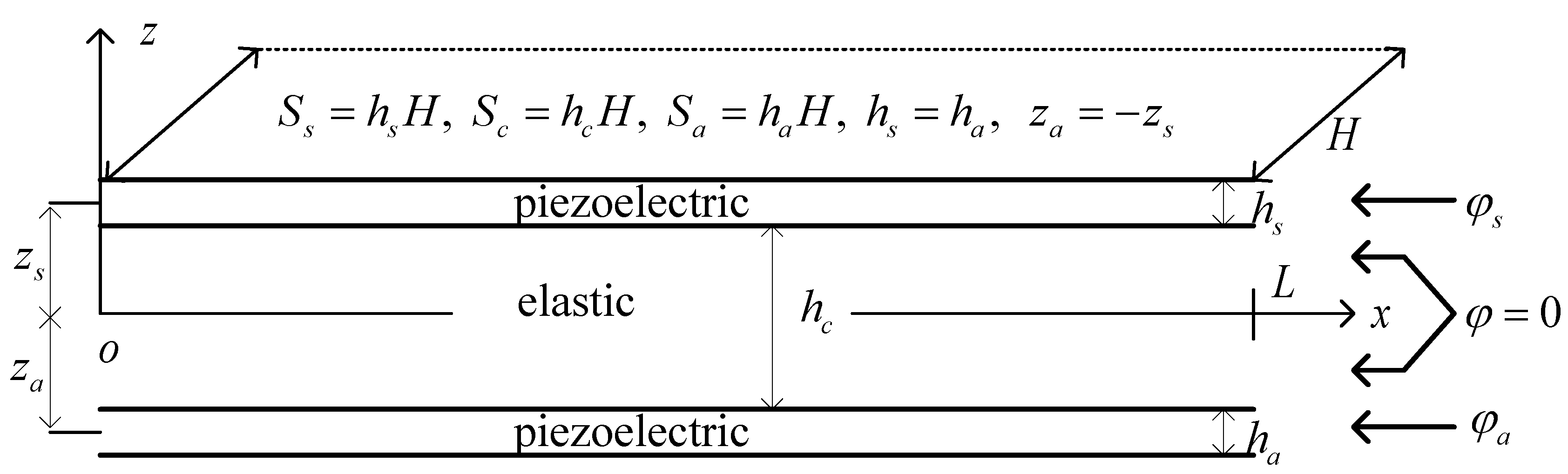
Figure 2.
Comparison of the three analytical methods on the amplitude-frequency responses of the S-S beam.
Figure 2.
Comparison of the three analytical methods on the amplitude-frequency responses of the S-S beam.
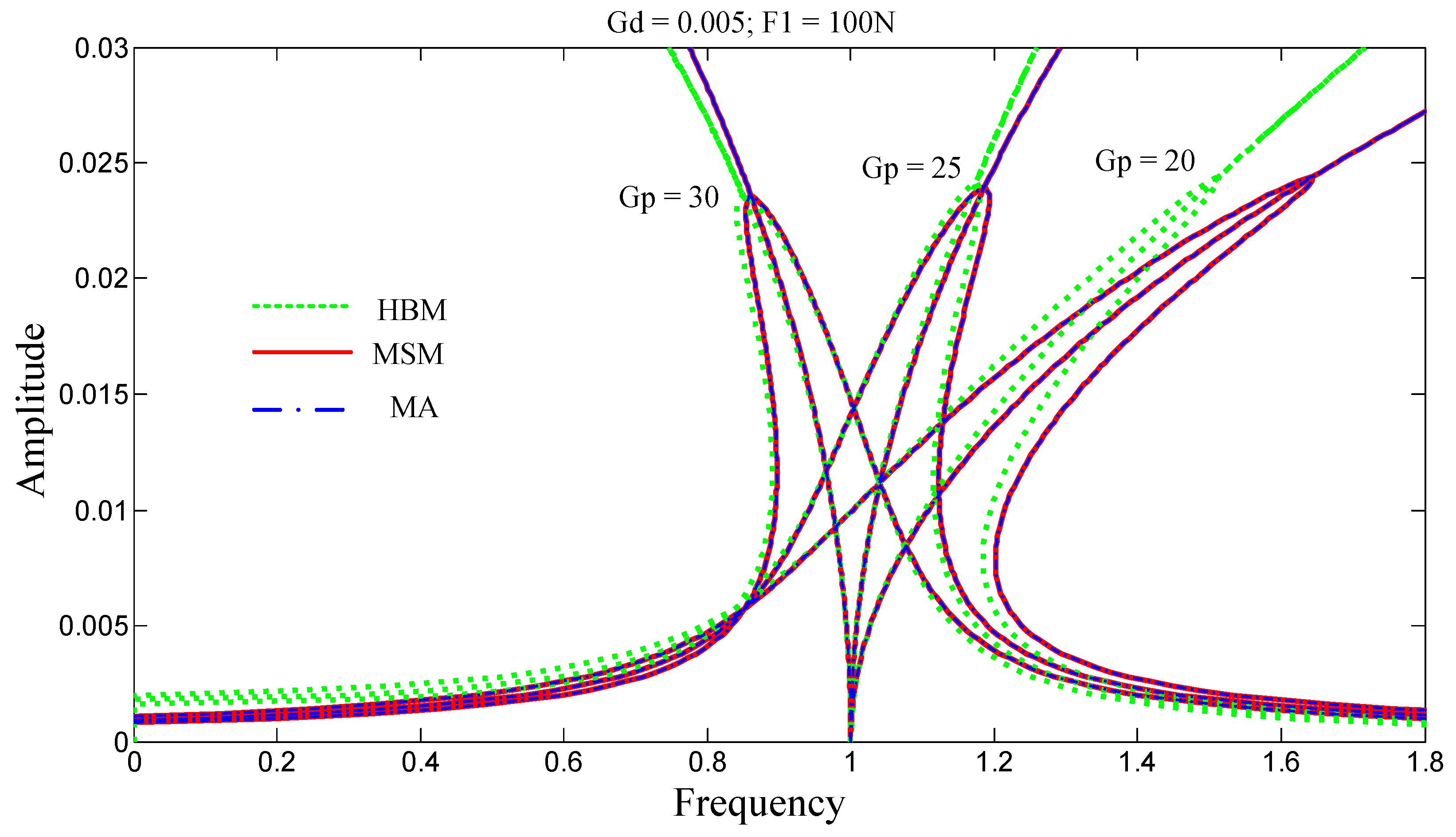
Figure 3.
Jumps in the increasing direction of frequencies.
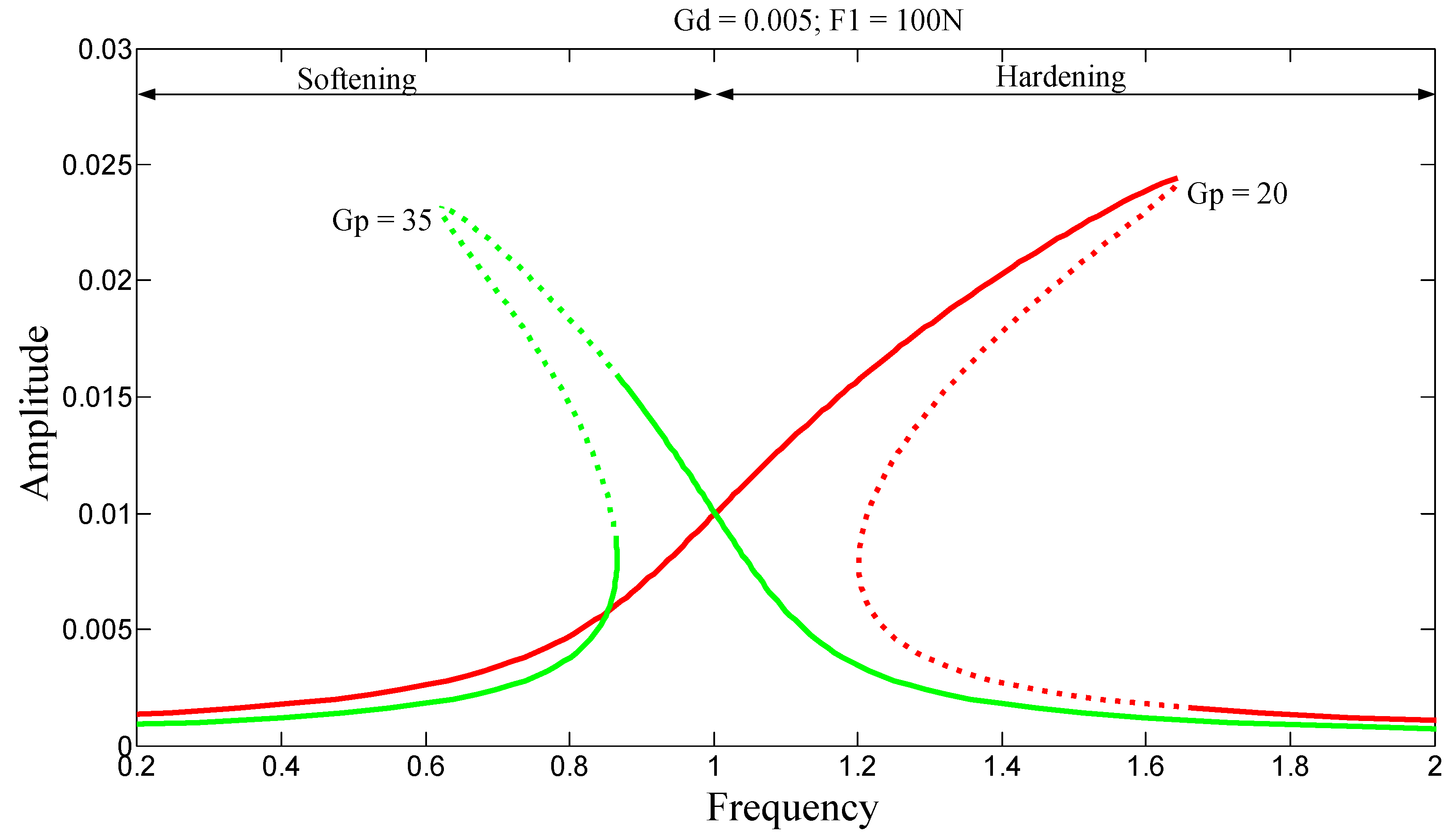
Figure 4.
Jumps in the decreasing direction of frequencies.
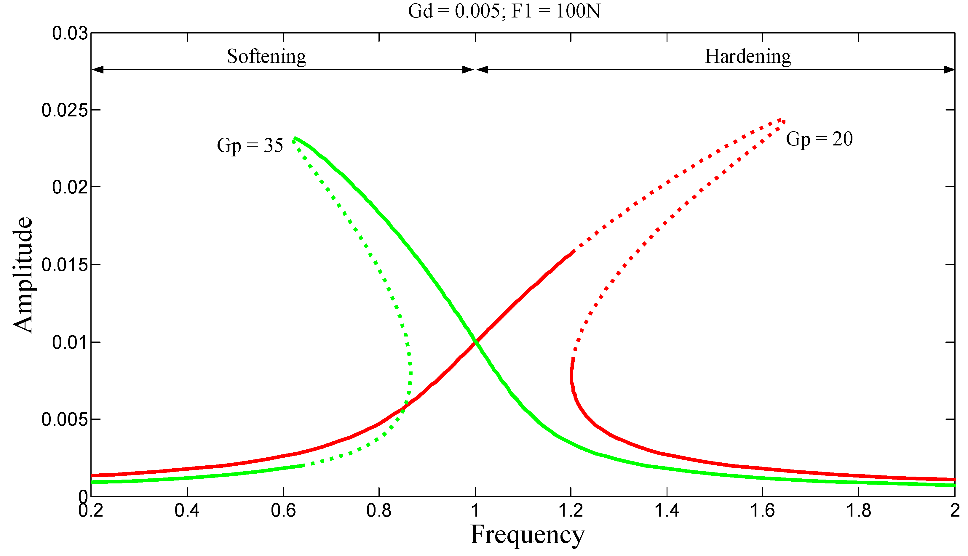
Figure 5.
Amplitude-frequency responses for the three boundary conditions.
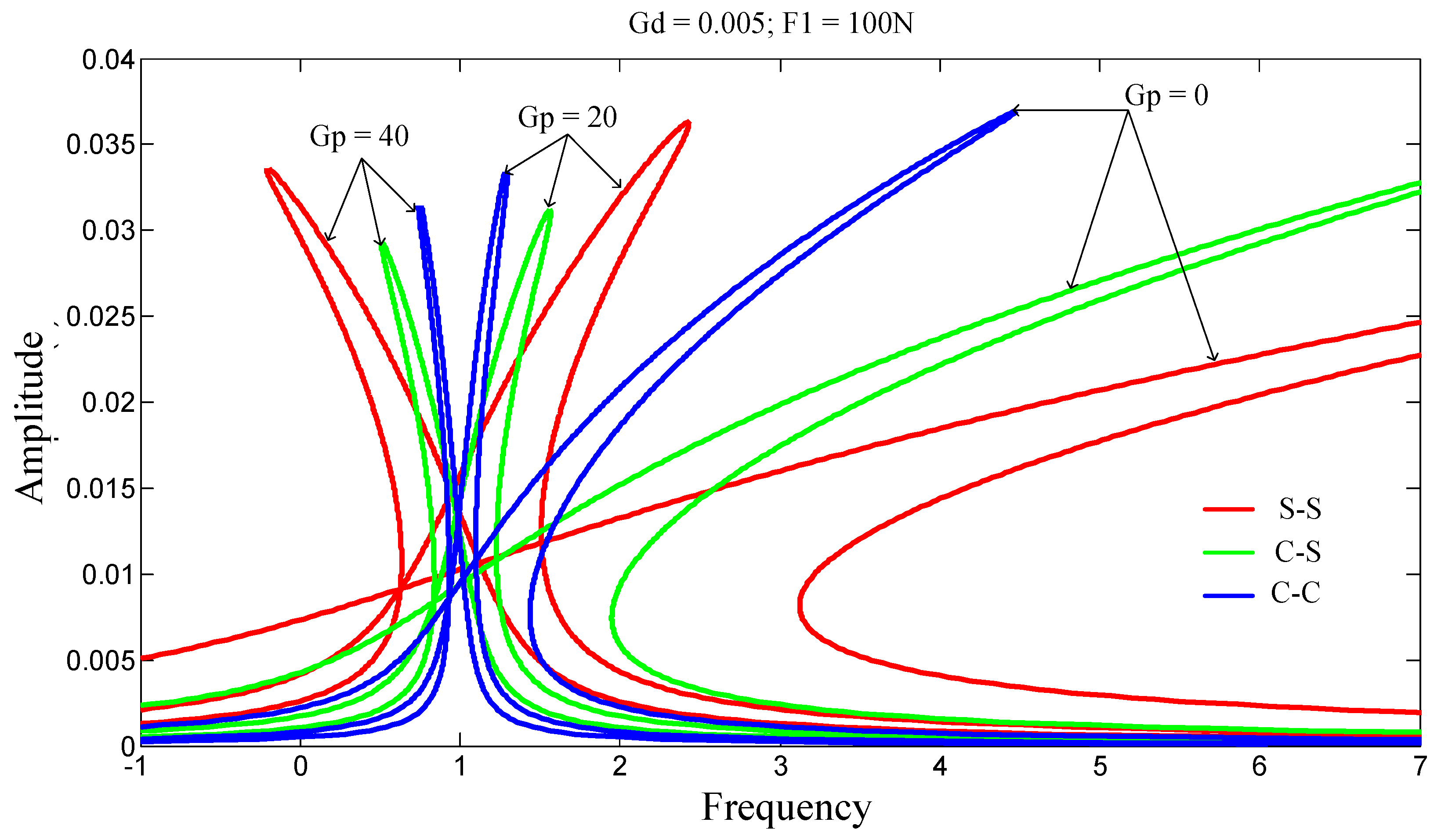
Figure 6.
Free nonlinear amplitude-frequency responses for the three boundary conditions.
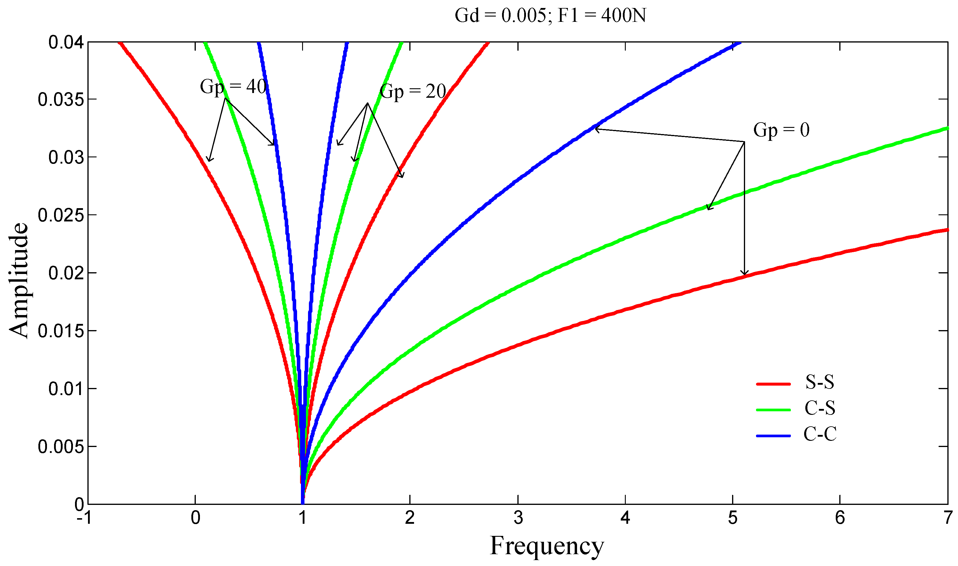
Figure 7.
Amplitude-frequency responses of the three boundary conditions.
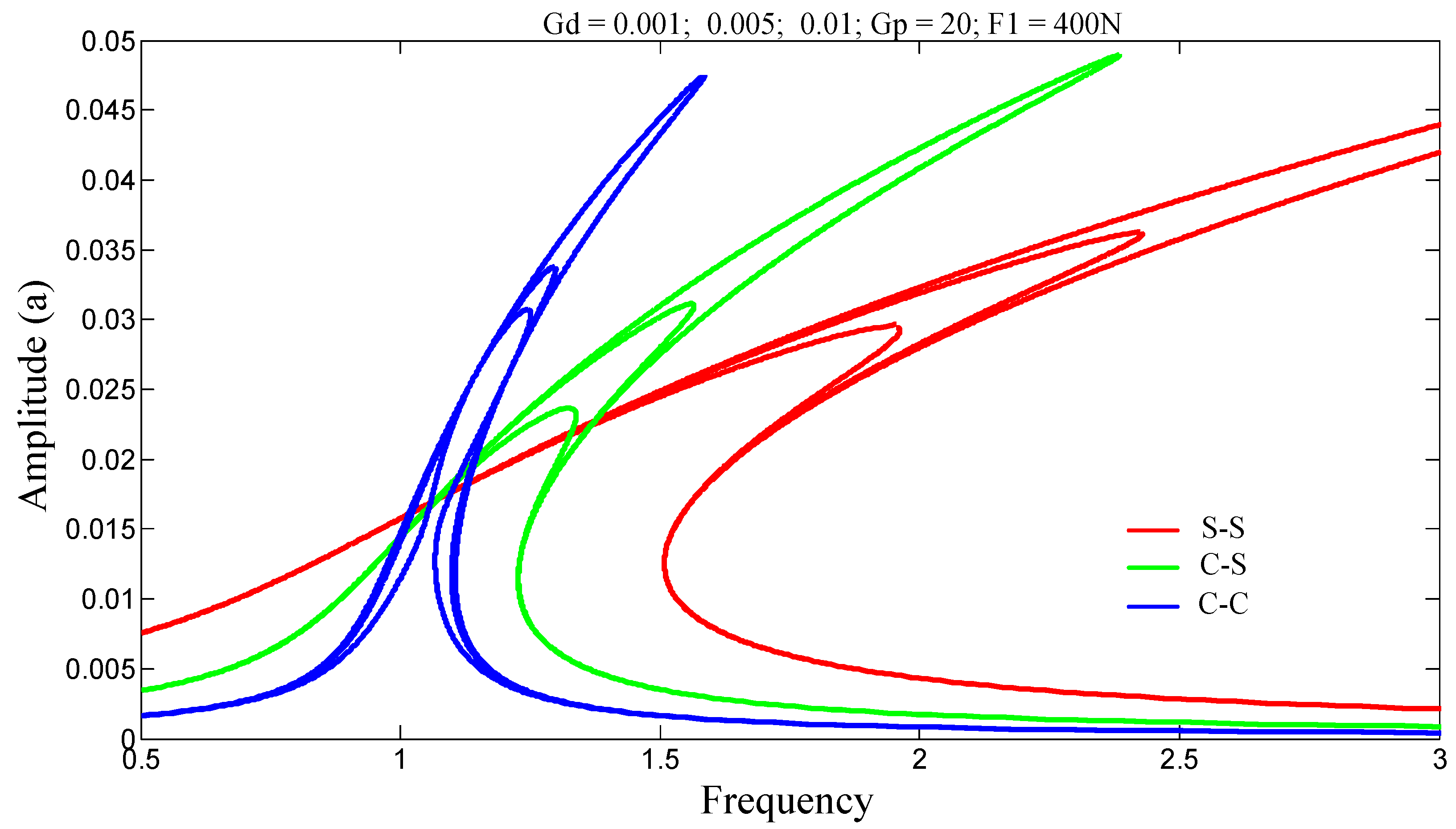
Figure 8.
Amplitude-frequency responses of the three boundary conditions.
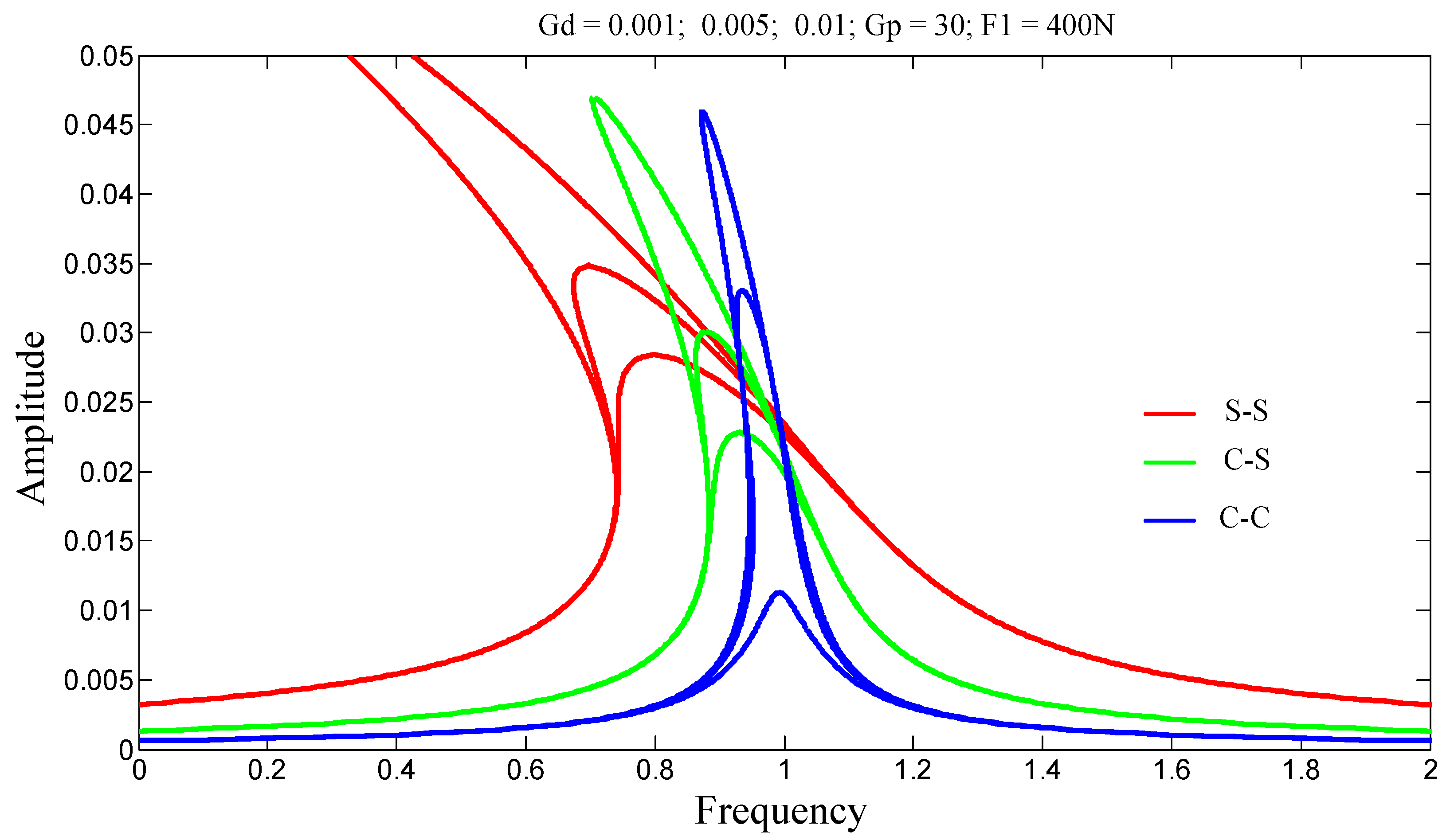
Figure 9.
Amplitude-frequency superharmonic responses for of beam S-S.
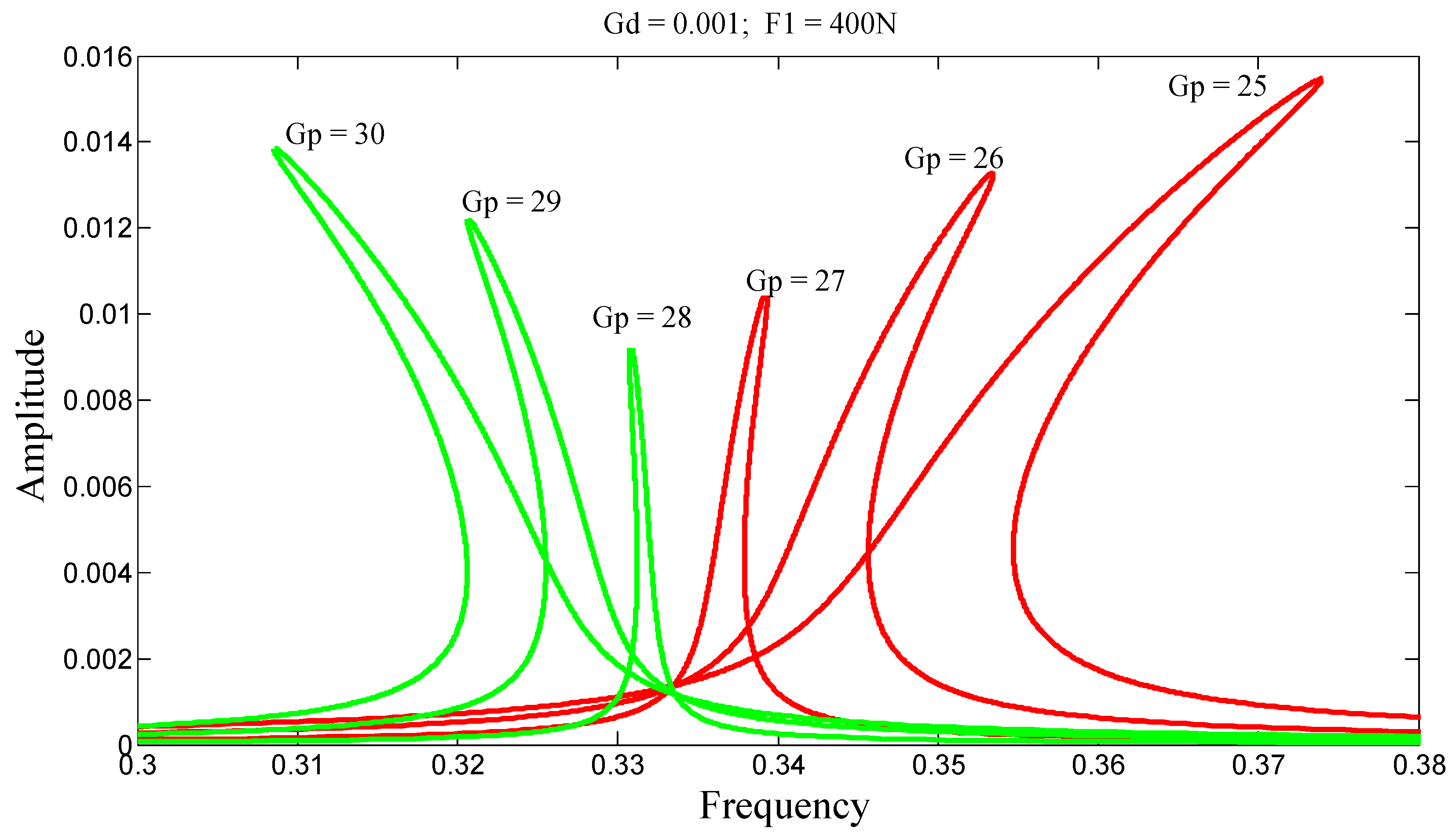
Figure 10.
Amplitude-frequency superharmonic responses for of beam S-S.
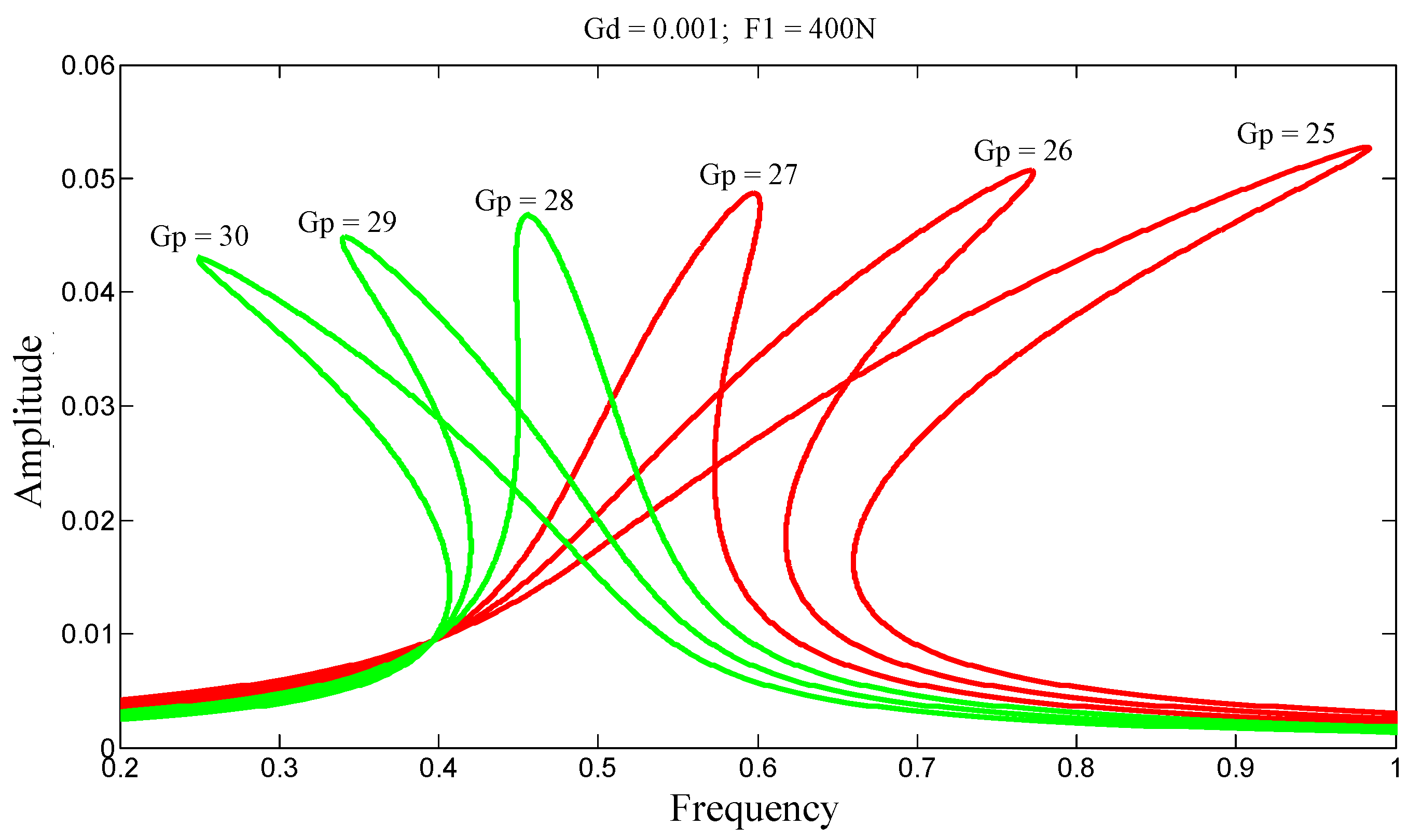
Figure 11.
Amplitude-frequency superharmonic responses for of beam C-S.
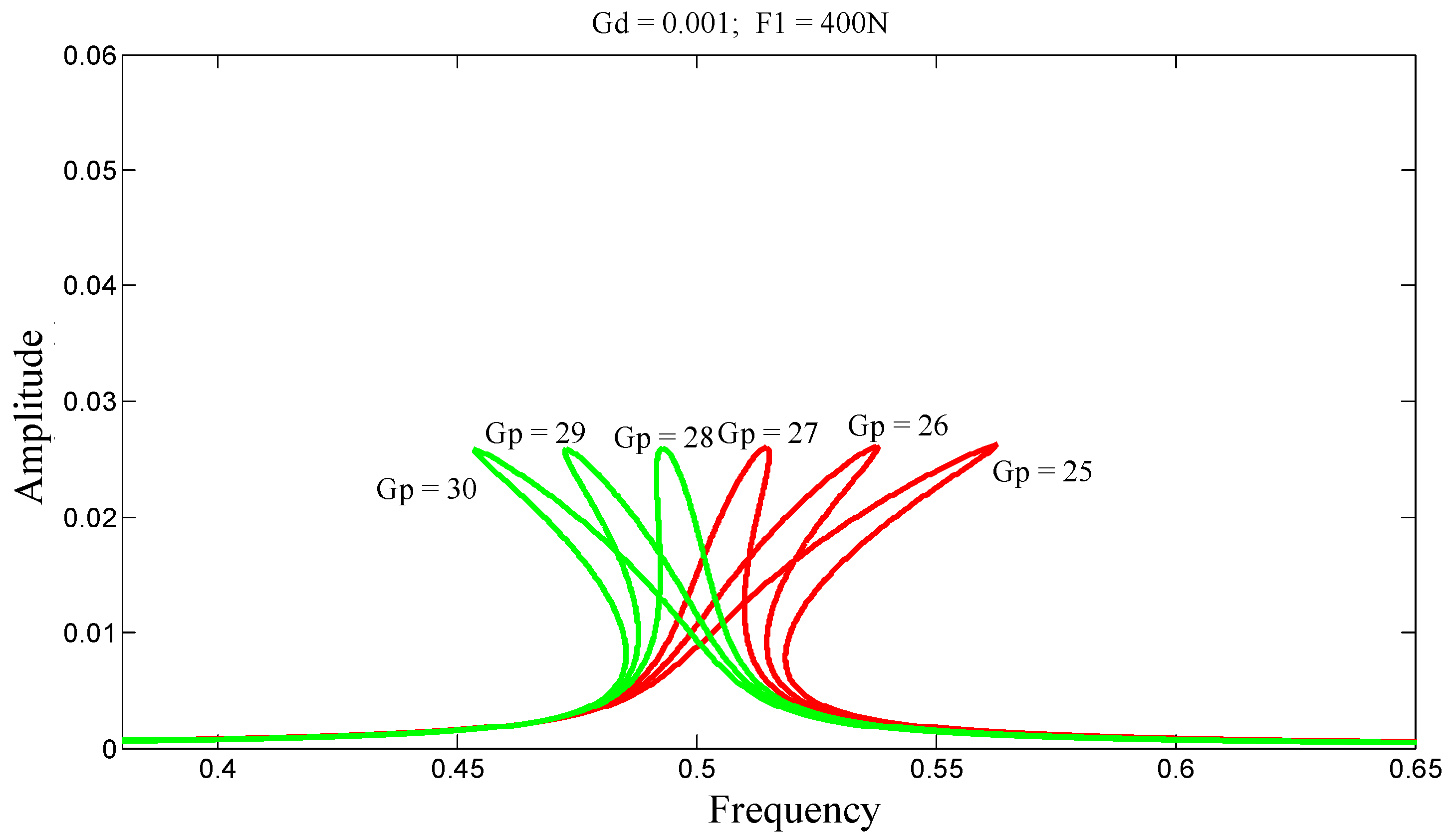
Figure 12.
Super-harmonic amplitude-frequency response for of the C-C beam.
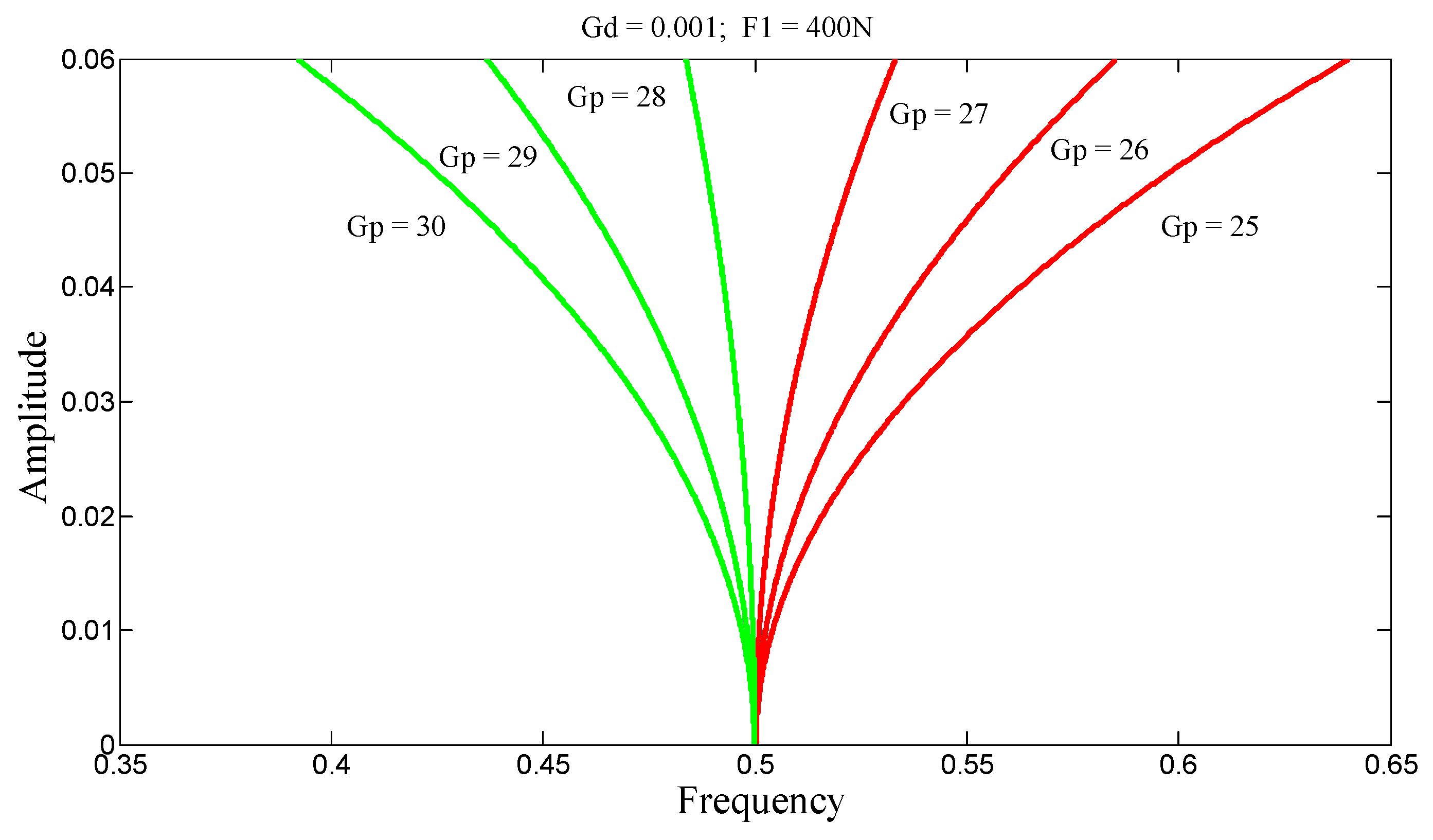
Figure 13.
Subharmonic amplitude-frequency responses for of S-S beam.

Figure 14.
Subharmonic amplitude-frequency responses for of S-S beam.
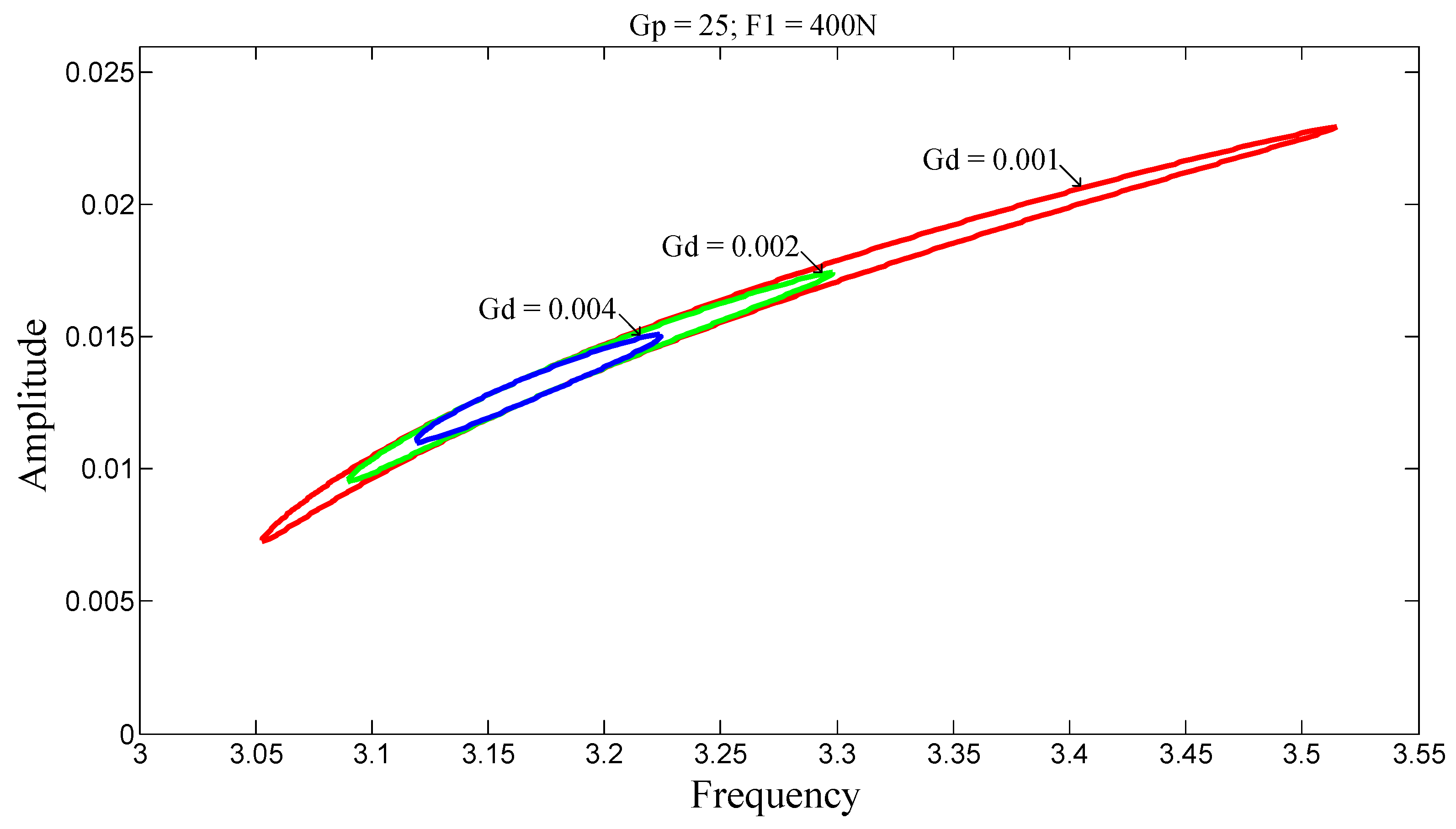
Figure 15.
Subharmonic amplitude-frequency responses for of C-S beam.
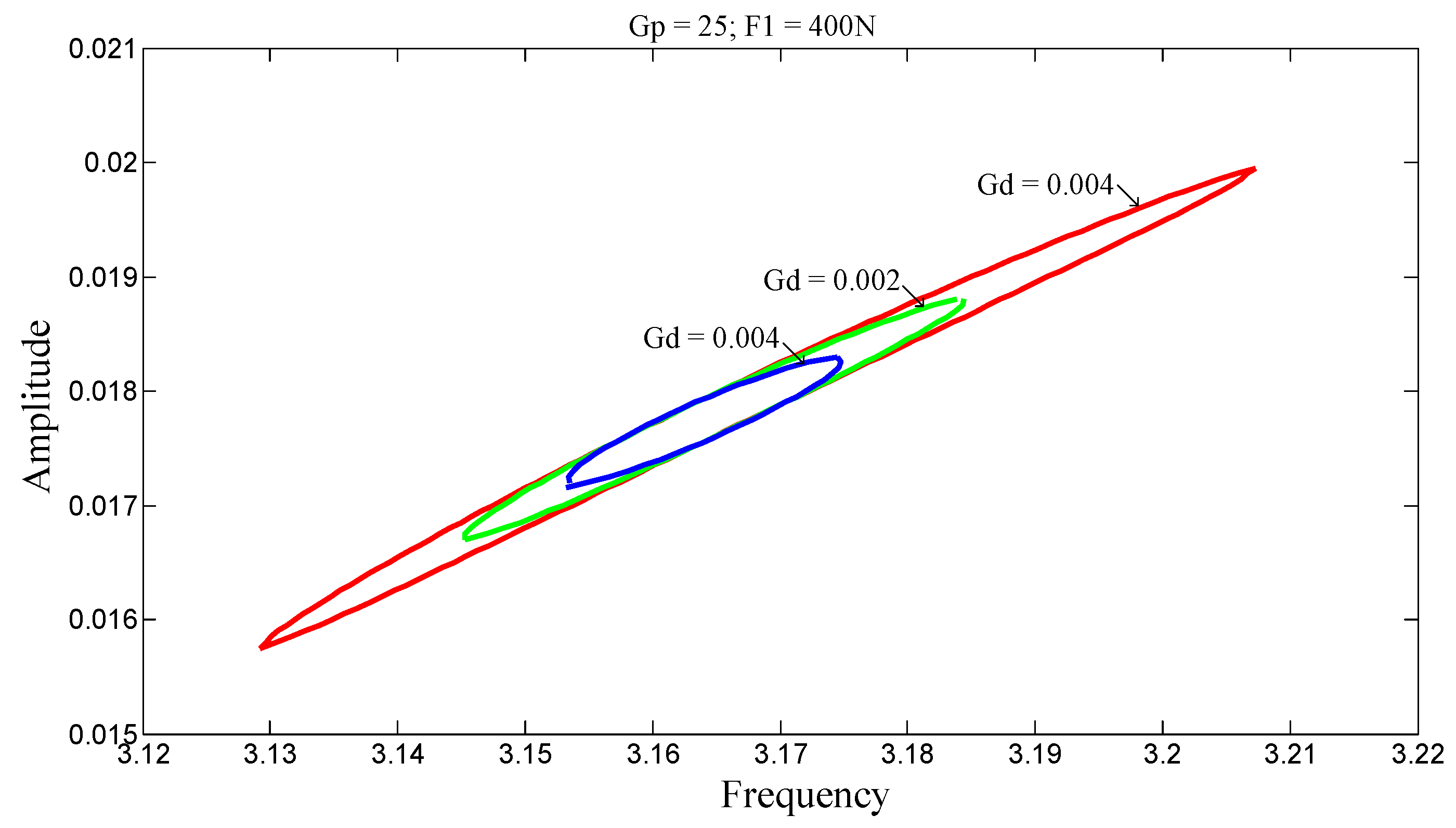
Figure 16.
Subharmonic amplitude-frequency responses for of S-S beam.
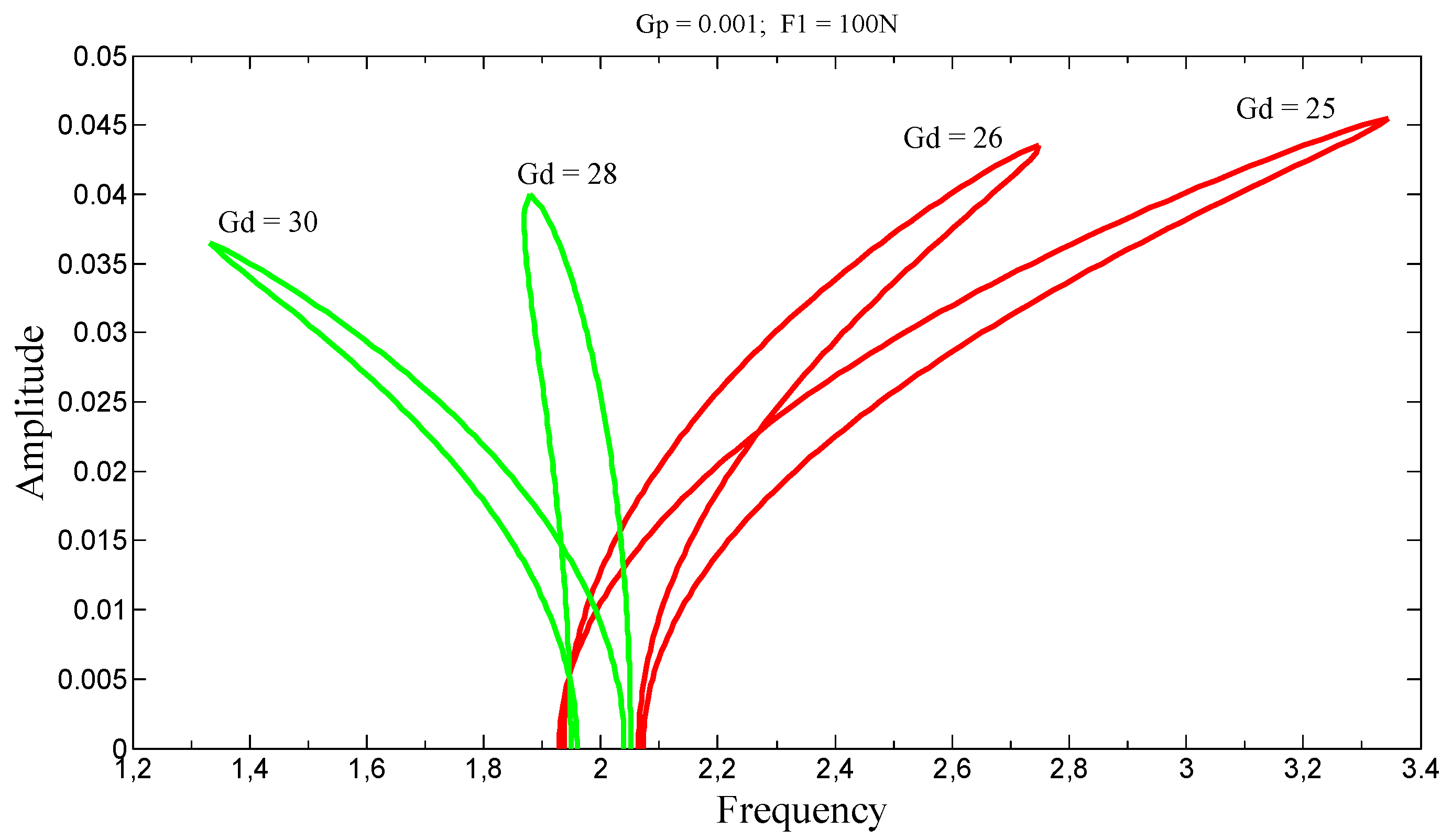
Figure 17.
Subharmonic Amplitude-Frequency Responses for of S-S Beam.
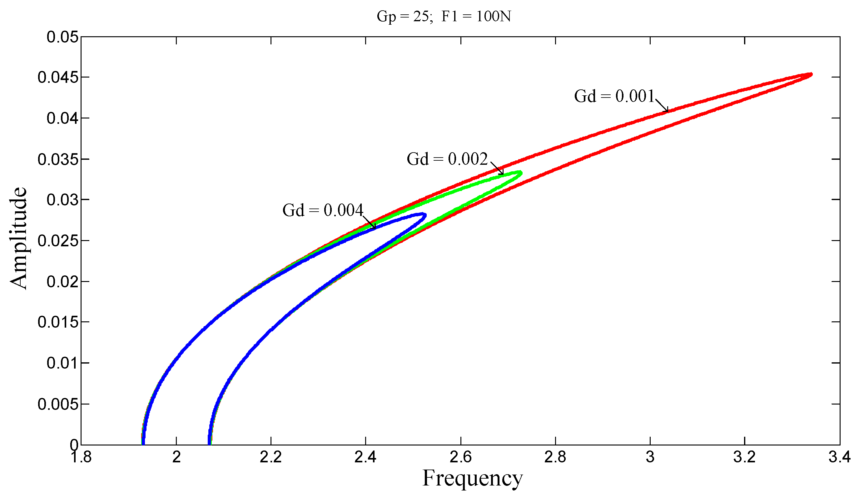
Figure 18.
Subharmonic amplitude-frequency responses for of C-C beam.
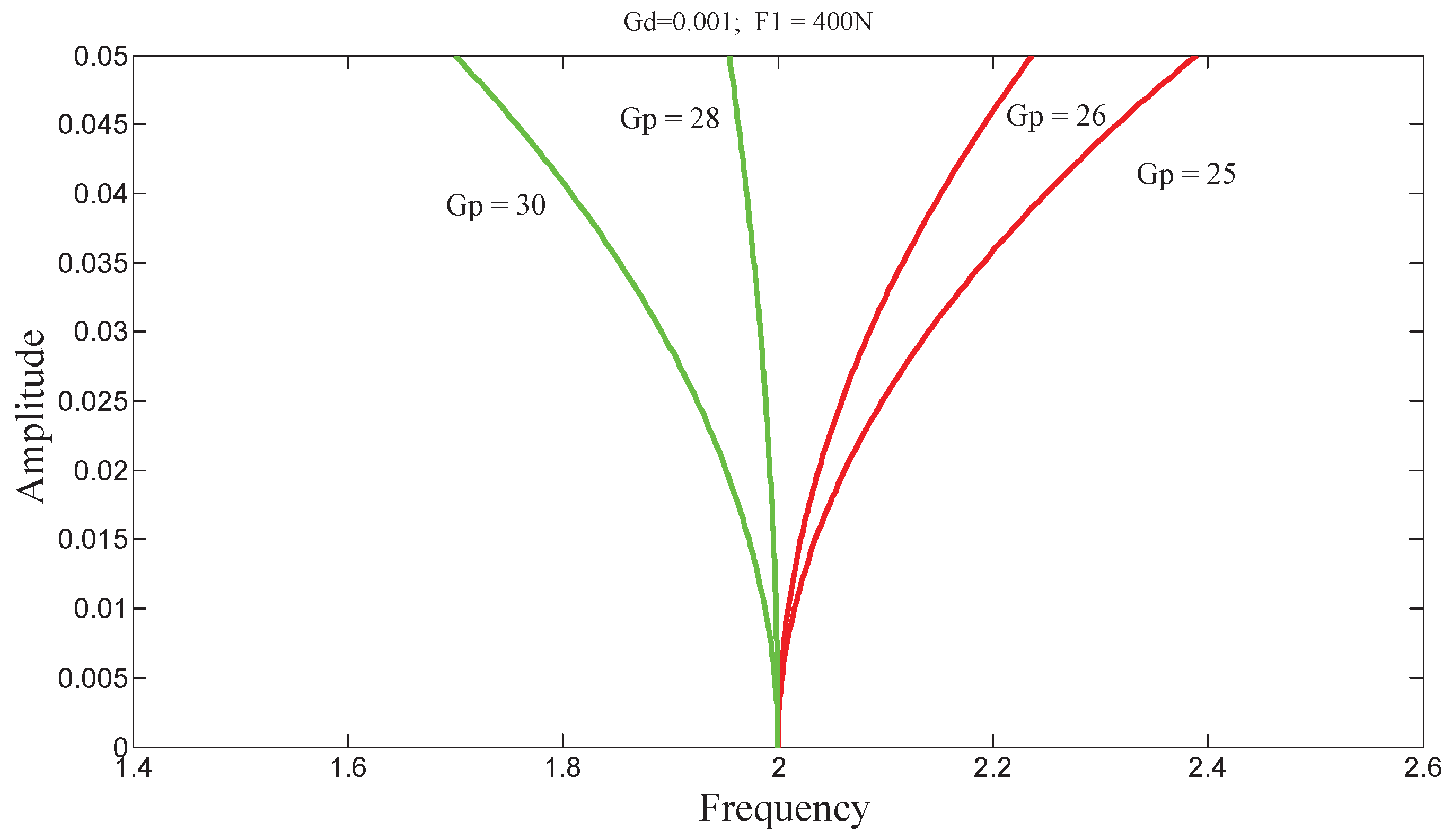

Table 1.
Geometric and material properties of the beam [12].
Table 1.
Geometric and material properties of the beam [12].
| Elastic layer | Piezoelectric layer | |
| L: Length (m) | 1 | 1 |
| H: Width (m) | ||
| h:Total thickness (h = 0.01) | ||
| Young’s modulus (Pa) | --- | |
| Density (Kg.m-3) | ||
| (Pa) | --- | |
| (C.m-2) | --- | |
| (F.m-1) | --- |
Table 2.
Coefficient values corresponding to the three boundary conditions [12].
Table 2.
Coefficient values corresponding to the three boundary conditions [12].
| S-S | C-S | C-C | |
Disclaimer/Publisher’s Note: The statements, opinions and data contained in all publications are solely those of the individual author(s) and contributor(s) and not of MDPI and/or the editor(s). MDPI and/or the editor(s) disclaim responsibility for any injury to people or property resulting from any ideas, methods, instructions or products referred to in the content. |
© 2025 by the authors. Licensee MDPI, Basel, Switzerland. This article is an open access article distributed under the terms and conditions of the Creative Commons Attribution (CC BY) license (http://creativecommons.org/licenses/by/4.0/).
Copyright: This open access article is published under a Creative Commons CC BY 4.0 license, which permit the free download, distribution, and reuse, provided that the author and preprint are cited in any reuse.


