
Submitted:
27 June 2025
Posted:
30 June 2025
You are already at the latest version
Abstract
The research investigates a composite beam consisting of two layers with different thicknesses and materials subjected to thermal and mechanical loads. Two cases of temperature loading are considered here: uniformly distributed temperature along the whole beam and linear distributed temperature along the beam thickness. A reduced model of the problem based on the first three beam’s normal modes is formulated. Additionally, a simplified one-mode reduction model is developed and solved analytically by the harmonic balance method (HBM). A comparison between the results of the three-mode reduction and the one-mode reduction models highlights the applicability and limitations of the latter. Differences in the resonance curves produced by these models are thoroughly examined. The reduced models are validated through comparison with results obtained by FEM. The detailed bifurcation diagrams are presented for the reduced three-degree-of-freedom (3-DOF) model. The analysis reveals phenomena such as loss of stability, mode interaction, buckling, and chaotic oscillations. These findings provide deeper insights into the dynamic behavior of thin composite beams subjected to mechanical and thermal loads, considering different variations of the temperature distribution.
Keywords:
nonlinear dynamics
; thermoelastic
; reduced model
; harmonic balance method
; analytical solution
; 3 mode reduction
; bifurcation diagrams
; resonance curves
; AUTO
1. Introduction
In recent decades, the dynamic behavior of thin-walled structures subjected to multiphysics fields has been the topic of increasing investigations. One explanation for this is the fast growth of micro- and nanotechnologies. Many micro-electromechanical and nanoelectromechanical systems are subjected to the influence of temperature, electrical, magnetic, or fluid fields. The interaction between mechanical fields and concomitant temperature, electrical, or other fields could be significant for the design, proper exploitation, and safety of structures. Often, the part of structures like sensors, membranes, and other micro-electronic devices are composite structures consisting of different materials. Such structures could be found in many other technological areas, such as the aerospace industry and chemical and energy technologies.
The thermomechanical issue is one of the most commonly encountered in engineering practice and is extensively researched in scientific literature. The classical books that present the basic problems of thermoelasticity are Boley and Weiner [1] and Nowacki [2].
Jones’ article [3] from 1963 was one of the first to consider the equations of motion for 3D beams, taking into account the temperature propagation along all beam dimensions. It used Euler-Bernoulli and Timoshenko beam theories but lacked numerical examples.
The evolution of dynamic thermoelastic investigations is closely related to the aerospace industry. A series of works studies the phenomena arising due to the combination of airflow, thermal, and mechanical fields acting on aerospace structures. Some of them are systematized in Torton’s book [4].
Other works (referenced as [5,6,7,8]) further explore flutter, buckling, and post-buckling behaviors in panels exposed to thermal environments. In [9], the influence of thermal gradients on flexural waves in bilayer beams, indicating potential for unbounded growth, is discussed.
An important characteristic of many works devoted to dynamic thermoelastic problems is that the subjects of investigation are often composite structures. Most often a homogenization procedure is applied for such structures and the problem is transformed to the one of a structure with generalized properties. For example, in [10,11] beams with functionally graded materials are considered and dynamic and stability problems are solved in the case of thermal loading. The dependence of material gradations on the critical buckling temperature is shown.
11In the previously mentioned references and many other papers treating dynamic thermoelastic issues, it is generally accepted that temperature influences the mechanical response. In contrast, the effect of structural motion on the temperature field is often overlooked. Some researchers have attempted to address this by solving the fully coupled problem, considering the simultaneous evolution of both mechanical and thermal fields [12,13,14,15,16,17]. For instance, the elastic-plastic behavior of beams exposed to various heat impacts is examined in [12], employing finite difference discretization to model both beam motion and temperature change and then solving the resulting system of ordinary differential equations for both fields concurrently. The nonlinear response of a clamped circular plate under thermal loads, including a constant and a harmonically varying temperature component, is analysed in [13]. The study in [14] focuses on the free vibrations and buckling of clamped annular plates subjected to axisymmetric in-plane thermal loads, investigating how different thermal and geometric parameters affect the system’s response. Integral transformations such as Fourier and Laplace are utilized to analyse the coupled thermoelastic vibrations of a Timoshenko beam under a step heat flux. In [15], Henkel and Laplace integral transformations are applied by Trajkovski and Ĉukić to explore the coupled vibrations of circular plates. Considering the differing propagation velocities of mechanical and temperature oscillations, an algorithm for a sequential approach to solving the equations of temperature propagation and beam vibrations is proposed in [16,17].
In [18], the equations of motion of a simply supported rectangular plate subjected to thermal and mechanical loads are transformed to three ordinary differential equations by the Galerkin method. The authors have computed numerically different nonlinear features as Poincare maps, phase plots, power spectra, and bifurcation diagrams. In [19], thermoelastic vibrations of a rotating micro-beam subjected to a laser pulse heat source and sinusoidal heating are considered. Mathematical modelling of the problem is developed using the Euler–Bernoulli beam theory and the generalized theory of thermal conductivity with three relaxation coefficients of time. The closed-form solutions are obtained by Laplace’s transform. Laplace’s transform is again applied in [20] to study the thermoelastic vibration of functionally graded nano-beams interacting with abrupt heat in nonclassical thermoelasticity with phase delays. In [21], the influence of temperature on vibrations of laminated layers made of two different materials is presented. Essentially, the object of the investigation can be considered as a functionally graded beam. The systematic and consistent studies of the nonlinear thermo-elastic dynamic behavior of plates are presented in [22,23,24,25,26,27,28].
In [22], vibrations of a laminated von Karman plate with a linear temperature distribution along the plate thickness are considered. The obtained continuous model is subjected to a minimum reduction via the Galerkin procedure, ending with a reduced model of three coupled ODEs. The linear distribution of the temperature along the plate thickness is accepted. In [23,24], the third-order plate theory is used for thermoelastic vibration of the laminated plate, as the variation in plate reference temperature varies according to cubic law. In [24], parametric investigation of the response is accomplished using bifurcation diagrams, phase portraits, and planar cross-sections of the four-dimensional basins of attraction to describe the model’s local and global dynamical behavior. Different scenarios induced by the boundary conditions are highlighted, along with the effect of varying modelling of temperature distribution on the system response. Assessing the possible occurrence, disappearance, or modification of mechanical buckling as a result of thermal influence is discussed in [25]. The effects of coupling are explored, and the crucial role played by the slow thermal transient evolution in modifying the fast, steady mechanical response is studied. The same authors studied nonlinear dynamics of plates subjected to thermal and mechanical loading in many different aspects [26,27]. In [27], the coupled problem of the nonlinear dynamics of composite plates is analytically treated, and the main bifurcation phenomena are studied. The resulting modulation equations and the steady-state mechanical and thermal responses are determined and compared with the numerical solutions.
The nonlinear dynamics of the coupled thermoelastic vibrations of isotropic and orthotropic plates are discussed [28,29], respectively. Various characteristics of nonlinear dynamics, including phase diagrams, Poincaré maps, fractal dimensions, bifurcation diagrams, power spectra, and Lyapunov exponents, are employed to describe the behaviour of these structures.
Laminated composite structures such as plates and beams are mostly used structures concerning dynamic thermoelasticity. One of the approaches in this case is to create a homogenized model of the structure using generalized properties of the material. Then, often reduced models are developed. This is a reasonable approach for layers with equal thickness and symmetrically disposed along the thickness. When homogenization cannot be applied, usually the finite elements method with 3 D elements is used. The cost for the computations, in this case, is very high. Other often-used structures considered objects of thermoelastic vibrations are functionally graded structures.
Reference [30] presents the analysis of the large amplitude thermo-mechanically coupled vibration of the simply supported orthotropic rectangular thin plate. The governing partial differential equation of the large deflection of thermo-mechanical coupling is derived and reduced to a set of three non-linear ordinary differential equations by the Galerkin method.
References [31,32] examine the effects of the coupled field on the response of functionally graded beams. Additionally, reference [33] investigates how moisture and temperature influence wave propagation in porous FG sandwich plates, emphasizing their impact on material expansion.
The authors of the present work modelled thermoelastic vibrations of circular plates in [34,35,36]. The complete model considers transversal and longitudinal displacements, taking into account the geometrical nonlinearity, shear deformation, inertia terms due to cross-section rotation, and thermal and mechanical loadings. Based on that model, temperature influences the first resonance zone and the bifurcation scenario, leading to buckling and chaotic oscillations, as presented in [34,35]. In [36], the reduced model is based on three-mode reduction and considers the effect of temperature, which is regarded as uniformly distributed through the plate. This paper demonstrates that all three modes are involved in the plate dynamics, and the elevated temperature essentially changes the plate’s response. The developed analytical model enables the detection of the buckling bifurcation point, post-buckling oscillations, and then a series of period-doubling bifurcations and zones of multistable solutions. A special case of composite structures is the bi-material beams. Usually, the two layers have quite different properties and thicknesses. Examples of such structures can be found as parts of many micro-electronic devices (MEMS), energy harvesting devices, etc. Bi-material Euler-Bernoulli beams with L and inverted T’s cracks are considered in [37]. An analytical method for determining dimensions of longitudinal cracks based on frequency measurements is developed. When such structures are subjected to mechanical and thermal loads, internal stresses could arise due to the difference in the mechanical and thermal properties of the structure. Most of the studies of the thermomechanical behaviour of the bi-material beams are devoted to their static states. Some consideration of the bending of bimaterial beams can be found as early as 1960 in the book of Boley and Weiner [1]. Later, many studies appear about bi-metallic beams’ deformation, stresses, and temperature distribution. The static thermoelastic deformation of composite beams is studied in [38,39,40,41]. The dynamic instabilities and transient vibrations of a bi-material beam with alternating magnetic fields and thermal loads are investigated in [42]. The authors used the Hamilton principle to deduce the equation of the beam’s vibration on the base of the Euler- Bernoulli theory. The equation of motion and the solution of thermal effect are obtained by superposing specific fundamental linear elastic stress states. The authors of this study investigated coupled vibrations of bi-material beams subjected to mechanical and thermal loads in [43] on the base of a reduced model and successful solution of the beam vibration equation and the temperature propagation equation. The influence of the elevated temperature on the nonlinear vibration, buckling and post-buckling behaviour of the beam has been presented. In the following paper [44], the model of homogenization of the beam has been applied to study in detail the dynamics of the beam in the frequency domain. Bifurcation analysis is performed, and conclusions about the possibility of arising multiple solutions, loss of stability, and bifurcation are presented. The reduced model is based on three modes reduction. The beam was somewhat thick, and getting the nonlinear response required large loads. The attempt for an experimental study approved this.
This work applies a similar approach but for a much thinner beam. In addition, the case of the temperature linearly distributed along the beam thickness is studied. This makes the reduced model more complicated and allows the discovery of new phenomena that arise due to temperature influence.
2. Mathematical Model
Figure 1 shows a composite beam consisting of two layers of different materials (Material 1 and Material 2) with thicknesses h1 and h2. The length of the beam is denoted with l, the width with b, and the thickness is h where h= h1+ h2 . The coordinate along axis of the interface between the layers is denoted with .
Assuming large displacements and applying the Timoshenko beam theory the strain and curvature-displacement relationships associated with the mid-axes can be expressed as:
and the strain vector is expressed as follows:
where is the transverse displacement, is the rotation angle, , according to the Timoshenko beam theory is a function describing the distribution of the shear strain along the beam thickness. The upper index 0 associates the strains and the curvature with the mid-axes.
Constitutive Equations
The relationships between the stress
and strains
, considering the temperature changes, are presented by the well-known equations:
where E(i) is the Young modulus of ith layer, G(i) is the corresponding shear modulus and is the coefficient of thermal expansion, T is current temperature, is the initial (environmental) constant temperature.
Equations of Motion
Starting from the equilibrium equations written for each layer and then following the procedure for homogenization described in [44] the following equations are obtained:
where c1 and c2 denote damping coefficients which are assumed to be proportional to the mass terms in front of the inertia terms. However, the inertia term in the longitudinal direction is neglected.
In Eq. (4) the following notations are introduced:
The equation describing the temperature propagation in the beam , without considering full coupling with the mechanical field is:
where are the heat capacity per unit volume and the thermal conductivity of ith material .
In this work, the temperature field is established and the temperature is uniformly distributed along the beam length. This means that the temperature does not change in time and the derivatives along x axis are zero. Therefore,
Concerning the distribution of the temperature along beam thickness two cases are considered: when —the temperature is elevated/lowered at the whole beam and the second case when the temperature is distributed along the beam thickness following the linear low:
The constants T0 and T1 are defined by the temperature boundary conditions.
The following boundary conditions about the temperature are defined:
where Td, Tup denote temperature on bottom (down) and upper beam surfaces.
In this case the coefficients in equation (12) are:
Considering that (see Figure 1):
it is easy to obtain that in the case of linear distribution of the temperature along the beam thickness:
while in the case of uniform temperature:
In the further text the notation ΔT means a difference between the beam and ambient temperatures.
Reduced Model
The mathematical model of the beam vibration is reduced by means the Galerkin procedure. To transform the partial differential equations into ordinary differential equations, the first three normal modes of the free vibrations of the homogenized beam are used as basis functions.
For convenience, the following dimensionless variables are introduced:
Then, equations (4) are transformed into the following equations:
The following notations are introduced in eq. (18)
and equations (7)-(9) are transformed into:
where d1 and d2 are damping coefficients.
For simplicity, in the text below “tilde” is omitted.
The solution of eq. (18 b,c) is sought in the form:
where Wi(x) and Ψi(x) are the normal modes of the beam vibrations—solution of the equations (18 b,c) with the zero right hand side and satisfying the boundary conditions.
Substituting eq. (14) into eq. (12 b, c) , using the orthogonality condition the following system of nonlinear ordinary differential equations is obtained:
In eq. (21) ωn are the natural frequencies of the linear elastic undamped bi-material Timoshenko beam, ξn are the modal damping parameters and:
Denoting:
then, substituting equation (20) into eq. (23) the following expression for the nonlinear force vector is determined:
For term, which accounts for the influence of temperature, the case of linear temperature distribution along the beam thickness is considered. When Tup=Td, obviously T1=0, and the beam is just subjected to elevated/lowered temperature ΔT.
Then
can be presented in the form
where
Therefore
Introducing the notations
and taking into account equations (22)-(30), the set of ODEs representing the three modes reduced model of the large amplitude thermoelastic vibrations of the bimaterial beam takes in the following final form:
where
Analytical Solutions for One Mode Reduction Model
In parallel with the 3 DOF model, a one-mode reduction model is created, and the obtained one-degree-of-freedom model is studied separately. The goals are to obtain an analytical solution to the equation of motion and compare the results with those obtained by the three-mode reduction model. Such a study could show the applicability and limits of the one-mode reduction model.
In this case the equation (31) is transformed to the following equation:
Then the harmonic balance method is applied, seeking the solution of (32) in the form:
where A1 and A2 are unknown amplitudes assumed as slow functions of time.
Introducing (34) into (33) and after the rejection small terms of higher order and balancing the first harmonics the set of modulation equations is obtained:
where: , .
For a steady state derivatives of amplitude are zero and therefore, after some analytical computations a cubic algebraic equation for the amplitude modulus is obtained:
Eq.(36) for amplitude
Stability of the analytical solution is based on Jacobian matrix defined on the basis of modulation equations (35) and then evaluated at the fixed point. If a real part of at least of one of the eigenvalue of the Jacobian matrix is positive then the solution is unstable otherwise it is stable or neutral. The details of the stability analysis is omitted here for the sake of simplicity.
This algebraic equation connects the excitation amplitude and frequency as well as temperature loading and allows obtaining the resonance curves and to perform other parametric studies of the bimaterial beam. The analytical solution obtained by HBM will be compared with the solution for the more advanced 3-mode model obtained directly from ODEs by the continuation method [45]. This comparison gives information about applicability of the one mode reduction and demonstrates the influence of the higher order modes on the beam dynamics, stability of the solutions and temperature influence.
Finite Element Model Validation
The developed model for the dynamic behaviour of the thermoelastic bimaterial beam is validated through finite element modelling. A three dimensional model of the bimaterial beam is created using the commercial software ANSYS [46]. The 3D finite element SOLID 226 is used for discretization of the beam. It is applicable for a lot of coupled fields analysis including Structural-Thermal. This element has twenty nodes with up to six degrees of freedom per node, which allows computations with a high accuracy.
The analyzed beam is composed of two layers: the bottom layer is made of aluminium alloy Al 1050 (Material 1) and the upper layer is made of copper C 12500 (Material 2). The dimensions of the beam, shown in Figure 1 are:
l = 0.4 m, h = 0.004 m, h1 = 0.003 m, h2 = 0.001 m, b = 0.02 m with material parameters of each layer:
E(1) = 7.0 × 10¹⁰ N/m2, ρ(1) = 2778 kg/m3, ν1 = 0.34, αT(1) = 23.9 × 10⁻⁶ 1/K
E(2) = 12.8 × 10¹⁰ N/m2, ρ(2) = 8940 kg/m3, ν2 = 0.34, αT(2) = 16.7 × 10⁻⁶ 1/K
The clamped-clamped boundary conditions which allow to express the nonlinear phenomena more clearly are assumed in the analysis.
The thickness of the beam is discretized into four layers: one layer for copper and three layers for aluminium. The finite element model includes a total of 32,000 elements and 157 889 nodes. The finite element discretization of the beam is illustrated in Figure 2.
The initial task is to perform modal analysis , to determine natural frequencies and the corresponding mode shapes.
The natural frequencies calculated by finite element model are compared with those obtained analytically for the reduced model, and the results are presented in Table 1.
The difference about 7% is also recorded in the previous paper using homogenization of the beam and the reduced model [44].
The second task is to compare forced response of the beam subjected to harmonic and thermal loads.
The solution of a hundred thousand nonlinear differential equations obtained after discretization of the problem requires essential computer resources – high computational power, disk space, and a long time to solve the problem. To get the time response of the bimaterial beam under mechanical loading and elevated temperature, for instance, for a period of one second, the program must be executed on a powerful desktop computer for several days. This fact is a limitation for consideration of a large number of cases studied by FEM. The main objective of the FEM computations is to illustrate the principal trends of the analyzed processes and to validate the mathematical model along with the results derived from it. The comparison of the time history diagrams of the bi-material beam subjected to harmonic loads with different amplitudes and different temperatures obtained by the reduced model of the beam and FE model are presented in Figure 3a, b, c.
The presented modal analysis and computed dynamic time responses for FE model and the reduced 3-modes model are in a good agreement. The observed deviation results from different assumptions in both models. However, the differences are acceptable and the correctness of the theoretical results confirmed. The more advanced bifurcation analysis and study of several interesting phenomena will be performed on the basis of the reduced models.
Nonlinear Dynamics Based on the 3 Modes Reduction Model
The equations of motion (31) of the reduced model of the thermo-elastic beam’s dynamics are solved numerically and the continuation technique with the predictor corrector steps is used to obtain bifurcation curves [48]. In this case the stability of the periodic solutions is determined by Floquet multipliers computed for the three ordinary differential equations of motion. The analysis starts with computation of the resonance curves and neglecting influence of the thermal loading, assuming Tup = 0, Td = 0. The curves are plotted for the case when the first mode is excited directly thus, we periodic force occurs on the right side of the first equation F1 = f1sinωt while F2 = 0, F3 = 0. This is the most important case because the first mode plays a crucial role in the dynamics. As the system is nonlinear the other modes are coupled and therefore they are indirectly activated as well. The three levels of excitation are selected to observe the beam’s response for the first q1 (Figure 4 a), second q2 (Figure 4 b), and third q3 (Figure 4 c) generalized coordinates. For the very small level of excitation amplitude (black curve) we observe almost a linear resonance response for q1 with negligible involvement of q2 and q3 coordinates.
As excitation increases the curves corresponding to q1 bend towards higher frequencies (red and green colour) and coordinates q2 and q3 are much more involved in the system’s response, however, with much larger values of coordinate q3 than q2 (note that in Figure 4 b scale is of 1 × 10⁻⁸ order). Participation of q3 coordinate is still limited but much larger in beam motion and increases with the increased level of mechanical loading.
Thus, considering that for moderate vibrations the modal interactions are rather negligible therefore the results based on the one mode reduction model can accurately capture the real system response, as presented in Section 4. Then, the solution can be determined analytically with very good accuracy.
More complicated dynamics occurs for large values of excitation, as presented in Figure 5. The instability on the resonance curves occurs for larger oscillation amplitudes, located close to the peak on the black resonance curve (f1 = 0.2×10⁻⁵) and in the middle of the red curve (f1 = 0.1×10⁻⁴), as presented in detail in zoom in Figure 5 (b). Consequently, the in stability is present for coordinate q2 in Figure 5 (c) and coordinate q3 in Figure 5 (d).
The question arises: what happens to the system if it works in the instability zone? In Figure 6 the solutions are determined around the frequency corresponding to bifurcation points BP1 and BP2. Starting from the bifurcation point BP1 an additional stable solution arises (red line) and this is a effect of a strong involvement of coordinate q2. From the bifurcation point, BP2, just unstable solutions arise, plotted by the blue dashed line. It means that for large vibrations the bifurcation points on the resonance curve occur and from them new solutions arise. The second vibration mode q2 is strongly activated. Out of this zone the first coordinate q1 interacts mainly with the third mode q3 while the second mode remains on a very small level. The phenomenon of the stability loss can be observed for the model with three degrees of freedom and it is not observed for the one mode reduction (Section 4).
The temperature influence in the vicinity of the first natural frequency is at first demonstrated for temperature uniformly distributed through the beam volume and for f1=0.1 x10⁻⁵ i.e. for relatively large vibrations but without the stability loss discussed above. In Figure 7 the black curve represents the reference resonance curve for ΔT=0. The ‘hot’ colour curves correspond to elevated temperature ΔT=5 (orange), ΔT=10 (pink), ΔT=15 (red), ΔT=20 (brown), and ‘cold’ colours for decreased temperatures ΔT=-10 (green), ΔT=-20 (blue). The decreased temperature below the reference ΔT=0 leads to a shift of the resonance curves towards higher frequencies and to the amplitudes reduction. The elevated temperature up to ΔT=15 reduces amplitudes and shifts the resonance curves towards lower frequencies. For ΔT=15, the beam buckles and a new branch arises from the bifurcation point. Further increase of temperature up to ΔT = 20 destroys the classical resonance curve and just post buckling oscillations exists (brown colour) with the partially stable branch and with unstable part for lower frequencies. The resonance curves are also shifted correspondingly for q2 (Figure 7 b) and q3 (Figure 7 c). Their involvement in the response is more evident if temperature is increased.
The influence of the temperature is also tested for twice larger mechanical loading for f1=0.2x10⁻⁵. The resonance curves are plotted for selected values of temperatures, again in ‘hot’ colours for positive and ‘cold’ colours for negative temperature (Figure 8 ). For temperature ∆T=-10, ∆T=-20 and ∆T=-30 the resonance curves are shifted towards higher frequencies presenting hardening and smaller values of amplitudes (∆T =-10 -green, ∆T =-20 -blue, ∆T =-30 -navy blue). In a case of elevated temperature the response becomes more complex. For ∆T = 10 the curve is shifted towards lower frequencies (orange curve) with an additional secondary resonance demonstrated by a peak on the resonance curve. Further temperature increase up to ∆T = 15 changes the curve essentially (red colour). First of all, two instability zones on the upper branch of the curve arise, at the beginning of the curve and close to the peak. The additional phenomenon is a bifurcation of the solution with two stable and one unstable branch which represents buckling of the beam in a positive or negative direction. The solutions for the post buckled state are fully stable in contrast to that presented in Figure 7 (a) for ∆T =15 where the post buckling instability zone exists.
For ∆T =20 the classical shape of the resonance curve is destroyed (magenta curve) and close to the top of upper branch additional stable solution arise coming from the strong interaction with the second mode as presented in Figure 8 (b). Values of q2 corresponding to other resonance curves are very small and therefore they are invisible in Figure 8 (b). The involvement of the third mode is presented in Figure 8(c) and it remains on the same order for all discussed cases.
Analysing the above results, presented in Figure 7 and Figure 8, we may conclude that the resonance characteristics are changed qualitatively if temperature is elevated above about ΔT=15. To check how the response changes if temperature is varied, the bifurcation diagrams against the elevated temperature ΔT are computed.
The bifurcation diagram of beam response is obtained for mechanical excitation level f1=0.1x10⁻⁵. and for five different frequencies selected around the resonance zone. The curves obtained for ω=0.05 -black, ω =0.06 -red, ω =0.07 -green, ω =0.08 -blue, ω =0.10 -orange get the shape reminding the frequency response curves (Figure 9 a). It is interesting that for all curves the bifurcation point BP occurs for the same temperature value about ΔT =14.35. The involvement of the coordinate q2 (Figure 9 b) is negligible while q3 is of one order smaller than q1 (Figure 9 c).
Detailed bifurcation analysis is conducted for fixed f1=0.1 x10⁻⁵ and ω =0.07 (Figure 10). Different branches of the solutions are indicated by dedicated colors. Starting from negative values of ∆T we follow black curve with periodic response corresponding to excitation frequency. For negative temperature coordinates q1, q2, q3 get very small values (Figure 10 c,d).
Approaching ∆T=0 and going forward the beam response increases up to maximal value at the turning point ∆T=15.43. The bifurcation curve reminds a stiffening resonance curve with three existing solutions.
Moving forward the periodic solution bifurcates at point BP (∆T=14.35) which is visible for the first and the third vibration modes in Figure 10 (a), (b) and (c), respectively. After buckling two branches arise (red curves). They are asymmetric which is better visible for larger values of ∆T. Around the elevated temperature ∆T=32 the second mode is strongly involved in the beam dynamics, as presented in Figure 10 (c).
Apart from the periodic solutions obtained by the continuation method also the isolated solutions shown in Figure 10 (a) by the green ‘isola’ above the red branch are obtained. The isolated solutions are partially stable and partially unstable (solid or dashed green line).
To demonstrate beam dynamics and coexisting solutions the time histories are plotted for the selected temperature values: ∆T =14, ∆T =16, ∆T =22, ∆T =35. The values of selected ∆T are indicated by thin vertical lines on the bifurcation diagram in Figure 10. The time histories are shown in Figure 11 (a)-(d). For ∆T=14 (Figure 11 a) we get two periodic solutions corresponding to the upper and lower branch in the bifurcation diagram (black curve). However, there is a third stable solution (green line) with about tripled period. This solution correspond to green ‘isola’ on bifurcation diagram. For ∆T =16 (Figure 11b), after the bifurcation point, post-buckling oscillations of the beam with positive (red) or negative (blue) offset take place. But again large amplitude oscillation (green colour) exists with tripled period and they correspond to oscillation between both buckled states. For larger temperature ∆T =22 just two small amplitude vibrations around buckled states exist, plotted by red and blue time histories in Figure 11(c). For this temperature the solutions of the ‘isola’ are unstable therefore the large amplitude oscillations presented by a green line in Figure 11(b) do not exist anymore. For larger temperature ∆T =35 four different post buckling vibrations are possible (Figure 11d). This is a result of the third and the second mode activation which is visible in Figure 10(c) and (d). It means that for ∆T =35 we obtain large and small amplitude oscillations around buckled states with positive (red) and negative (blue) offset.
The proposed model enables to study an effect of a heat transfer linearly distributed through the beam thickness assuming the temperature of the up (Tup) and down (Td) beam’s surfaces. The resonance curves for different temperature gradient are shown in Figure 12. The reference resonance curve for Tup=0, Td =0 is plotted in black. For temperature gradient Tup =10, Td =0 the resonance curve (red colour) is shifted into lower frequencies, for the opposite temperature gradient Tup =0, Td =10 we observe the same trend but the shift is smaller (orange curve). This phenomenon comes from asymmetric geometric and material properties of the beam. In a case of negative temperature, by putting Tup =-10, Td =0 the resonance curve is shifted towards higher frequencies (green curve) and for Tup =0, Td =-10 again the shift is smaller (blue curve).
Similar analysis is repeated for larger temperature gradient by assuming temperatures on upper and bottom surfaces with opposite signs. The resonance curves in Figure 13 are computed for Tup =15, Td =-15 (black), Tup =30, Td =-30 (red), Tup =50, Td =-50 (green). Comparing with the reference curve Tup =0, Td =0 plotted in grey, in all cases the curves are shifted towards lower frequencies when the temperature gradient is increased.
It should be noted that for the studied above temperature gradients the beam’s buckling does not occur. Even for large temperature difference Tup =50, Td =-50 the curve is just slightly more shifted. This is a result of two opposite effects: positive temperature on the upper part of the beam and negative on the lower part which compensate each other. For the elevated temperature when the beam is uniformly heated the buckling occurs at ∆T = 14.35.
To observe a difference in the bifurcation scenario we select Tup as a bifurcation parameter while temperature of the bottom surface is fixed, Td =0 (Figure 14). Then Tup temperature is varied from about Tup =-25 up to about Tup =82. We can distinguish pre-buckling solutions (black), post-buckling (red) and isolated solutions (green). The bifurcation diagram against elevated temperature ∆T plotted in Figure 10 is now repeated as reference in Figure 14 by a thin grey line. The bifurcation diagram against Tup shows much stronger stiffening nature and the bifurcation point of buckling takes larger value Tup =27.44 (red) comparing to BP indicated in grey. Furthermore, the post bucking solutions and isolated green solutions are shifted towards higher temperatures. Nevertheless, the solutions for linearly distributed temperature demonstrate qualitative similarities with the elevated temperature of the beam.
Applicability of One Mode Reduction
In Figure 15, the results obtained by the 1DoF model using the same data as the one used to obtain Figure 4a by the 3DoF model are shown. As one can see, the results are in a perfect agreement. Obviously, for these low levels of the load amplitudes and ∆T = 0, the 1DoF model is enough to obtain correct results.
Results shown in Figure 16 correspond to the case presented in Figure 5. The amplitude of the loading is much bigger than in the previous case. These lead to essential changes in the resonance curves obtained by the different models. The amplitudes of vibrations in the case of the 1DoF model are bigger but more essential is the fact that the more 3DOF model predicts instability of the upper branch of the resonance curve. This cannot be obtained by 1DoF model.
Most of the curves shown in Figure 17 and plotted for different temperatures are very similar to those shown in Figure 7a, but for ∆T=15, the additional instability obtained by the 3DoF model cannot be predicted. Of course, the interaction of modes and partially stable and partially unstable isolated solutions are obtained by the 3DoF model for higher temperatures, and the 1DoF model cannot get them.
f1 = 0.1×10⁻⁵ and different values of elevated temperature: ∆T = 0-black, ∆T = 5 orange,
∆T = 10-pink, ∆T = 15-red, ∆T = 20-brown, ∆T = −10-green, ∆T = −20-blue;
If one compares Figure 18 with Figure 8, the same conclusion can be made – multiple solutions (ΔT=15) and many instabilities in the solutions cannot be detected by the 1 DoF model.
Bifurcation diagrams shown in Figure 19 show similar behavior of the beam response q1 as the one in Figure 9a, but the values of the maximal amplitudes are different, and some instability at the upper branches of the curve for the maximal temperature is not detected by the 1 DoF model.
In the vicinity of the first natural frequency and fixed mechanical loading, f1 = 0.1×10⁻⁵, and different excitation frequencies: ω = 0.05-black, ω = 0.06-red, ω = 0.07-green, ω =0.08-blue, ω = 0.10-orange.
For the case of a linear distribution of the temperature along the beam thickness, the results obtained analytically are similar to those shown in Figure 12 a. The asymmetry due to the geometric and material properties of the layers is also confirmed analytically.
Conclusions
In this study, a nonlinear thermo-elastic model of a bimaterial beam is developed, considering mechanical and thermal boundary conditions. The model enables the study of the influence of mechanical and thermal loading considering the heat linearly distributed through the beam thickness. The model is validated through comparison with finite element analysis, including vibration modes, frequencies, and time response under periodic excitation for clamped-clamped boundary conditions.
The impact of mechanical and thermal loading is investigated for the three degrees of freedom model and then compared with the analytical solutions obtained by the harmonic balance method from the reduced one degree of freedom model. The models with one and three degrees of freedom exhibited strong agreement for relatively small periodic forces, demonstrating that higher vibration modes (second and third) have a minimal effect on the system’s behavior. The resonance curves showed stiffening, particularly at larger amplitudes. However, for large amplitude oscillations of the bi-material beam, the instability zone occurs on the frequency response curve because of a strong interaction of the second and the third vibration modes, resulting in additional solutions. The reduced model based on the one mode cannot detect this phenomenon. Moreover, the increased temperature leads to bifurcation and bimaterial beam buckling with asymmetric post-buckling oscillations and strong modal interactions. Then, even four stable solutions may exist with small or large amplitude oscillations around each of the two buckled states and also the isolated solution of large amplitude with oscillations between two buckled states may occur. The shift of the resonance curves and nonlinear stiffening effect is observed in the case of linearly distributed temperature through the beam thickness. However, if a sign of the temperature gradient is changed, the shift of the curve is different. Increasing the temperature of the upper beam surface and fixing the temperature of the bottom, a stronger hardening phenomenon is obtained compared with the case of elevated temperature. The bifurcation point occurs at a higher temperature, and thus, post-buckling dynamics is shifted as well. Although, the beam response is in qualitative agreement with the response for the beam under elevated temperature.
In conclusion, the analysis underscores the importance of considering mechanical and thermal effects, particularly at elevated temperatures, to accurately predict the dynamic behavior of bi-material beams under periodic loading. The findings highlight the significance of higher vibration modes, temperature distribution, and post-buckling dynamics, contributing valuable insights into the design and performance of such systems.
Funding
This work was accomplished with financial support from the Bulgarian research fund, grant KP-06-N72/7, 2023 and first and third authors acknolege this support. Research of the second author was funded in part by National Science Centre, Poland, Grant No. 2021/41/B/ST8/03190.
References
- Boley:, B. , Weiner, J. Theory of thermal stresses. Wiley, New York, 1960.
- W. Nowacki, Thermoelasticity, ed. 2, rev. & enlarged Edition, Pergamon Press and Polish Scientific Publishers, Oxford a.o and Warszawa, 1986.
- J.P. Jones. Thermoelastic vibtrations of beams. AEROSPACE CORPORATION El Segundo, California, Contract No. AF 04(695)-169, 20 February 1963.
- E. A. Thornton, Thermal Structures for Aerospace Applications, American Institute of Aeronautics and Astronautics, Reston, 1996.
- Radu, N. Udrescu, Aerothermoelastic behaviour of skin panels exposed to alternating thermal excitation. European Congress on Computational Methods in Applied Sciences and Engineering ECCOMAS 2000 Barcelona, 11-14 September 2000, ECCOMAS, 1-11.
- Mei, C. , Abdel-Motagaly, K., Chen R. Review of nonlinear panel flutter at supersonic and hypersonic speeds. Appl. Mech. Rev 1999, 52, 321–332. [Google Scholar] [CrossRef]
- Travis, L. Turnery, Z. W. Zhongz and Chuh Mei. Finite element analysis of the random response suppression of composite panels at elevated temperatures using shape memory alloy fibers. NASA-aiaa-94-1324.
- Shi, Y. , Lee R.Y.Y, Mei C. Thermal postbuckling of composite plates using the finite element modal coordinate method. AIAA Journal 1999, 37, 1035–1032. [Google Scholar]
- H. Hao, C. Scola, F. Semperlotti,. Flexural-mode solid-state thermoacoustics. Mechanical Systems and Signal Processing 2021, 148, 107143. [Google Scholar] [CrossRef]
- Ye Tang, Qian Ding. Nonlinear vibration analysis of a bi-directional functionally graded beam under hygro-thermal loads. Composite Structures 2019, 225, 111076. [Google Scholar] [CrossRef]
- Ye Tang, Shun Zhong, Tianzhi Yang and Qian Ding. Interaction Between Thermal Field and Two-Dimensional Functionally Graded Materials: A Structural Mechanical Example. International Journal of Applied Mechanics 2019, 11, 1950099. [Google Scholar] [CrossRef]
- Karagiozova, D. , Manoach, E. Coupling effects in an elastic-plastic beam subjected to heat impact. Nuclear Engineering and Design 1992, 135, 267–276. [Google Scholar] [CrossRef]
- Nayfeh, A. Faris W. Dynamic behavior of Circular structural elements under thermal loading. Paper AIAA 2003-1618. 4th AIAA/ASME/ASCE/AHS Structures, Structural Dynamics, and Materials Conference, April 2003,Norflock, Virginia.
- Arafat, H. , Faris W, Nayfeh A.. Vibrations and buckling of annular and circular plates subjected to a thermal load. Paper AIAA 2003-1927. 4th AIAA/ASME/ASCE/AHS Structures, Structural Dynamics, and Materials Conference, April 2003,Norflock, Virginia.
- Trajkovski, D. , Ĉukić R. A coupled problem of thermoelastic vibrations of a circular plate with exact boundary conditions. Mech. Res. Commun. 1999, 26, 217–224. [Google Scholar] [CrossRef]
- Manoach, E. , Large amplitude vibrations of Timoshenko beams subjected to thermal loading. Proceedings of 8th International Conference on Recent Advances in Structural Dynamics, Southampton, UK. CD-paper 39 (2003). [Google Scholar]
- Manoach, E. , Ribeiro, P. Coupled, thermoelastic, large amplitude vibrations of Timoshenko beams. Int. J. Mechanical Sciences 2004, 46, 1589–1606. [Google Scholar] [CrossRef]
- Yen-Liang Yeha, Cha’o-Kuang Chenb, Hsin-Yi La. Chaotic and bifurcation dynamics for a simply supportedrectangular plate of thermo-mechanical couplingin large deflection. Chaos, Solitons and Fractals 2002, 13, 1493–1506. [Google Scholar] [CrossRef]
- Tiwari, R. , Abouelregal, A.E., Shivay, O.N. et al. Thermoelastic vibrations in electro-mechanical resonators based on rotating microbeams exposed to laser heat under generalized thermoelasticity with three relaxation times. Mech Time-Depend Mater 2024, 28, 423–447. [Google Scholar] [CrossRef]
- Ahmed E Abouelregal. Computational analysis of thermoelastic vibrations of functionally graded nonlocal nanobeam excited by thermal shock. Journal of Vibration and Control 30. [CrossRef]
- Pazera, E. Jędrysiak, J. Effect of Temperature on Vibrations of Laminated Layer Vibrations in Physical Systems. 2018, 29, 2018032. [Google Scholar]
- Saetta, E. , Rega, G.: Unified 2D continuous and reduced order modeling of thermomechanically coupled laminated plate for nonlinear vibrations. Meccanica 2014, 49, 1723–1749. [Google Scholar] [CrossRef]
- Saetta, E. , Rega, G.: Third order thermomechanically coupled laminated plate: 2D nonlinear modeling, minimal reduction, and transient/post-buckled dynamics under different thermal excitations. Compos. Struct. 2017, 174, 420–441. [Google Scholar] [CrossRef]
- Valeria Settimi. Eduardo Saetta. Giuseppe Rega. Nonlinear dynamics of a third-order reduced model of thermomechanically coupled plate under different thermal excitations. Meccanica 2020. [CrossRef]
- Settimi, V. , Rega, G., Saetta, E. Avoiding/inducing dynamic buckling in a thermomechanically coupled plate: A local and global analysis of slow/fast response. Proceedings of the Royal Society A: Mathematical, Physical and Engineering Sciences 2018, 474, 20180206. [Google Scholar] [CrossRef]
- Settimi, V. , Saetta, E., Rega, G. Local and global nonlinear dynamics of thermomechanically coupled composite plates in passive thermal regime. Nonlinear Dyn 2018, 93, 167–187. [Google Scholar] [CrossRef]
- Settimi, V. , Rega, G. Asymptotic formulation of the nonlinear bifurcation scenarios in thermomechanically coupled plates Nonlinear Dyn. 2023, 5941–5962. [Google Scholar] [CrossRef]
- Y. -L. Yeh, C.-K. Chen, H.-Y. Lai, Chaotic and bifurcation dynamics for a simply supported rectangular plate of thermo-mechanical coupling in large deflection. Chaos Solitons Fractals 2002, 13, 1493–1506. [Google Scholar] [CrossRef]
- Yeh, YL. Chaotic and bifurcation dynamic behavior of a simply supported rectangular orthotropic plate with thermo-mechanical coupling. Chaos Solitons Fractals 2005, 24, 1243–55. [Google Scholar] [CrossRef]
- Yeh, YL. The effect of thermo-mechanical coupling for a simply supported orthotropic rectangular plate on nonlinear dynamics. Thin-Walled Struct 2005, 43, 1277–95. [Google Scholar] [CrossRef]
- Ye Tang, Qian Ding. Nonlinear vibration analysis of a bi-directional functionally graded beam under hygro-thermal loads. Composite Structures 2019, 225, 111076. [Google Scholar] [CrossRef]
- Ye Tang, Shun Zhong, Tianzhi Yang and Qian Ding. Interaction Between Thermal Field and Two-Dimensional Functionally Graded Materials: A Structural Mechanical Example. International Journal of Applied Mechanics 2019, 11, 1950099. [Google Scholar] [CrossRef]
- S. I. Tahir, A. Chikh, A. Tounsi, M.A. Al-Osta, S.U. Al-Dulaijan, M.M. Al-Zahrani, Wave propagation analysis of a ceramic–metal functionally graded sandwich plate with different porosity distributions in a hygro-thermal environment, Compos. Struct. 2021, 269, 114030. [Google Scholar] [CrossRef]
- Warminska, E. Manoach, J. Warminski, Dynamics of a circular Mindlin plate under mechanical loading and elevated temperature. MATEC Web of 400 Conferences 2016, 83, 05013. [Google Scholar] [CrossRef]
- Warminska, E. Manoach, J. Warminski, A reduced model of a thermoelastic nonlinear circular plate. MATEC Web of Conferences 2018, 148, 06001. [Google Scholar] [CrossRef]
- Manoach, E, Warminska, A., Warminski, J., Doneva, S.. A reduced multimodal thermoelastic model of a circular Mindlin plate. Int. J Mechanical Science 2019, 153-154, 479–489. [CrossRef]
- J. T. Ravi, S. Nidhan, N. Muthu, S.K. Maiti,Analytical and experimental studies on detection of longitudinal, L and inverted T cracks in isotropic and bi-material beams based on changes in natural frequencies. Mechanical Systems and Signal Processing 2018, 101, 67–96. [Google Scholar] [CrossRef]
- Shang Y F, Ye X Y, Feng J Y. Theoretical analysis and simulation of thermoelastic deformation of bimorph microbeams. Sci China Tech Sci 2013, 56, 1715–1722. [Google Scholar] [CrossRef]
- Carpinteri, A. , Pungo N Thermal loading in multi-layered and/or functionally graded materials: residual stress field, delamination, fatigue and related size effects. Int. J. Solids Struct 2006, 43, 828–841. [Google Scholar] [CrossRef]
- Carpinteri, A. , Paggi M. Thermo-elastic mismatch in nonhomogeneous beams. J Eng Math 2008, 61, 371–384. [Google Scholar] [CrossRef]
- Srinivasan, P. , Mark, S. Spearing Effect of Heat Transfer on Materials Selection for Bi-material Electrothermal Actuators. Journal of microelectromechanical systems 2008, 17, 653–667. [Google Scholar] [CrossRef]
- Guan-Yuan, Wu. The analysis of dynamic instability of a bimaterial beam with alternating magnetic fields and thermal loads. J. Sound and Vibration 2009, 327, 197–210. [Google Scholar]
- Manoach, E. Doneva, S., Warminski, J.. Coupled, Thermo-elastic, Large Amplitude Vibration of Bi-material Beams. Advanced Structured Materials, 134, Springer Science + Business Media, 2020, 227-242.
- Manoach, E. , Warminski, J., Kloda, L., Warminska, A., Doneva, S. Nonlinear vibrations of a bi-material beam under thermal and mechanical loadings. Mechanical Systems and Signal Processing 2022, 177, 109127. [Google Scholar] [CrossRef]
- AUTO: Software for continuation and bifurcation problems in ordinary differential equations, http://cmvl.cs.concordia.ca/auto/.
- ANSYS.com.
Figure 1.
The geometrical scheme of the beam model.
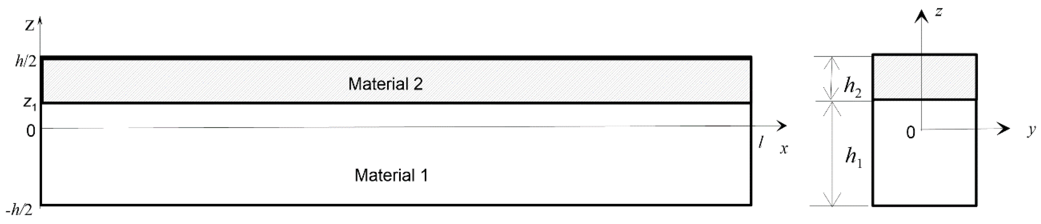
Figure 2.
Discretisation of the beam model.
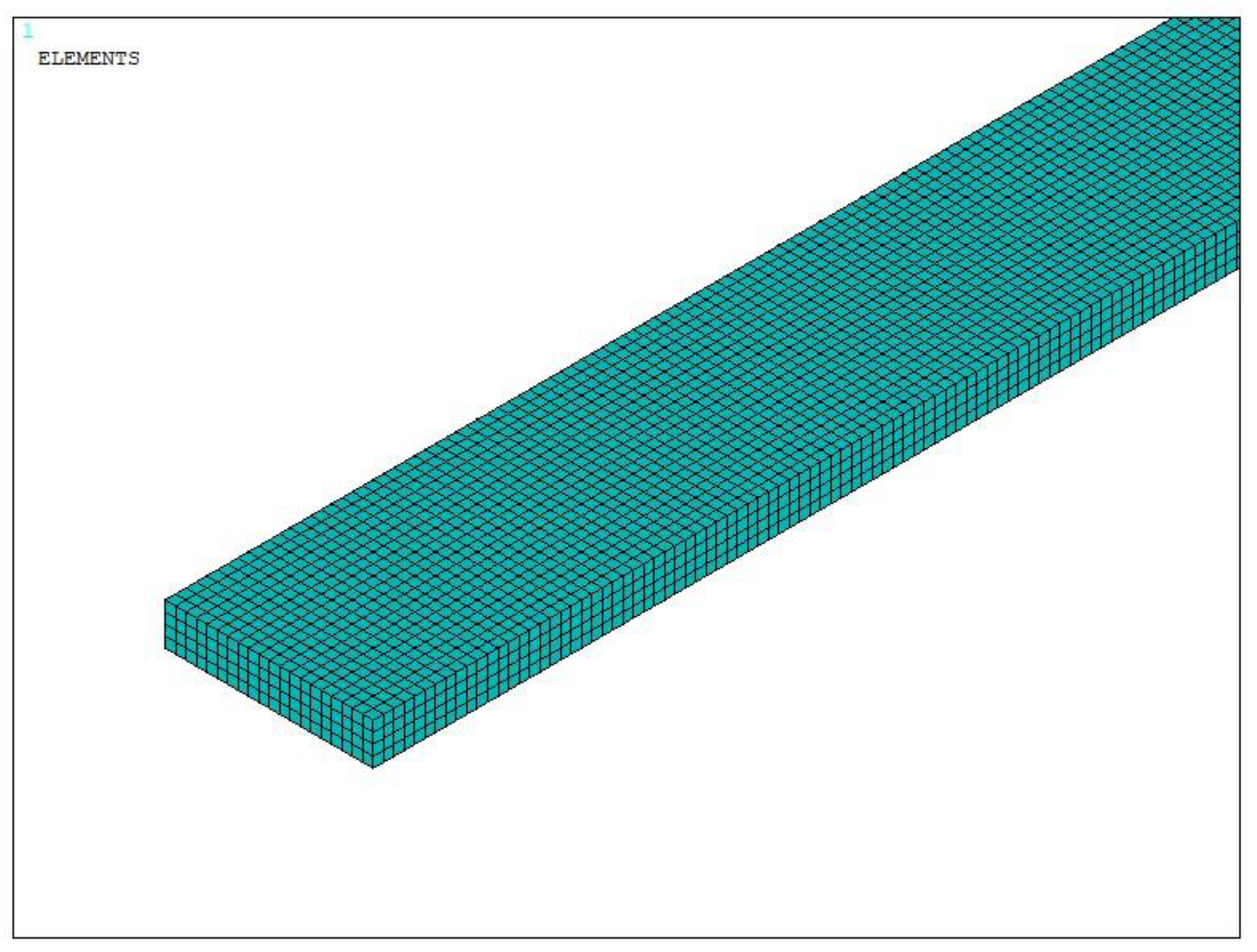
Figure 3.
a Time history diagram of the response of the beam centre – red colour ANSYS, blue colour – reduced model (3 mode reduction). ΔT=5, P=5000 N/m2, ωe=130 rad/s. b Time history diagram of the response of the beam centre – red colour ANSYS, blue colour – reduced model (3 mode reduction). ΔT=10, P=500 N/m2, ωe=130 rad/s. c Time history diagram of the response of the bi-material beam subjected to harmonic loading P=5000 , ωe=130 rad/s ΔT=10-comparison between the reduced model and FE model. Black colour – reduced model; Red colour—ANSYS.
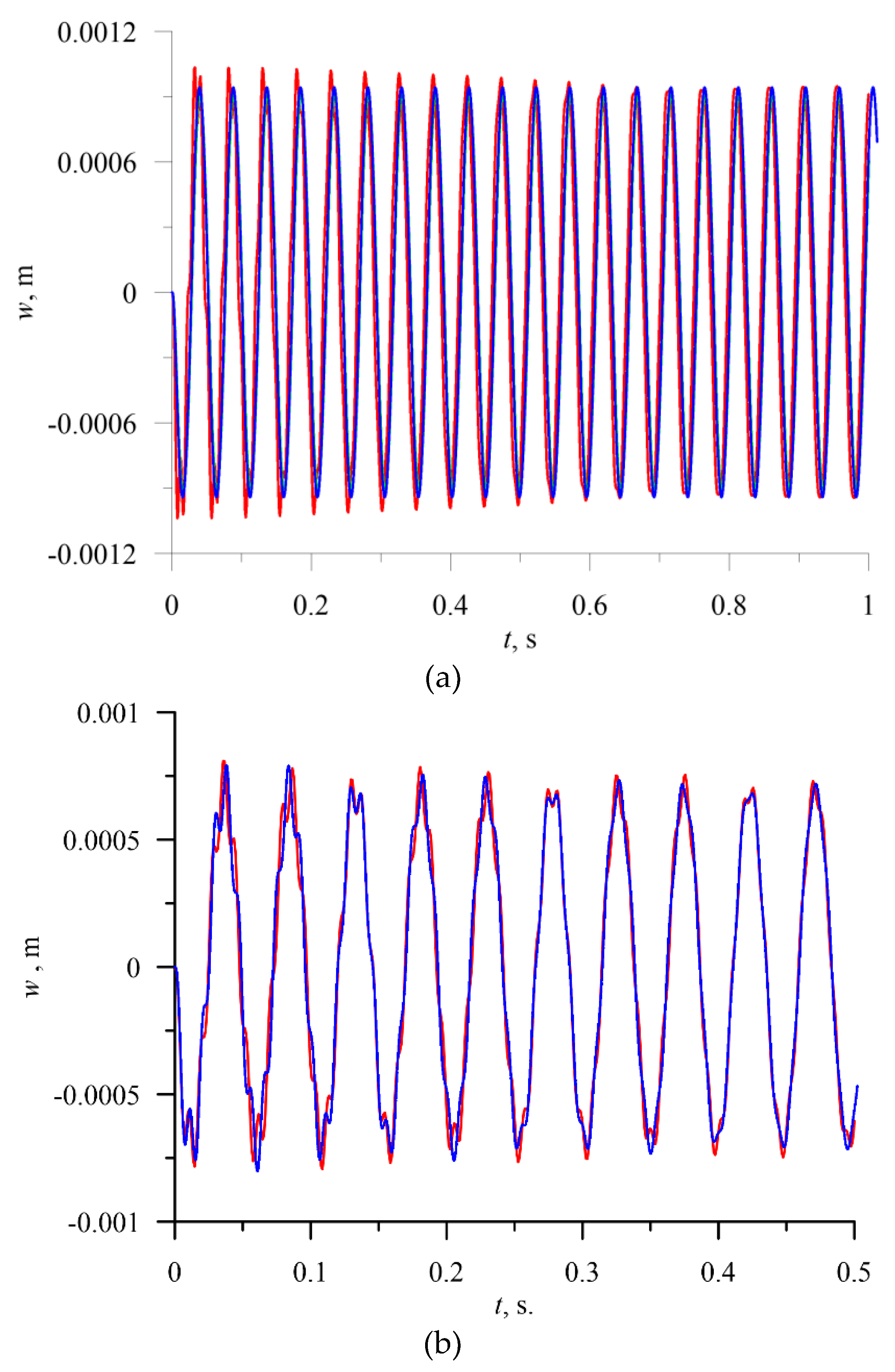
Figure 4.
Resonance curves around the first natural frequency for large mechanical loading, f1=0.1x10⁻⁶-black, f1=0.5x10⁻⁶-red, f1=0.1x10⁻⁵-green; ∆T = 0; (a) coordinate q1,.(b) coordinate q2, (c) coordinate q3.
Figure 4.
Resonance curves around the first natural frequency for large mechanical loading, f1=0.1x10⁻⁶-black, f1=0.5x10⁻⁶-red, f1=0.1x10⁻⁵-green; ∆T = 0; (a) coordinate q1,.(b) coordinate q2, (c) coordinate q3.
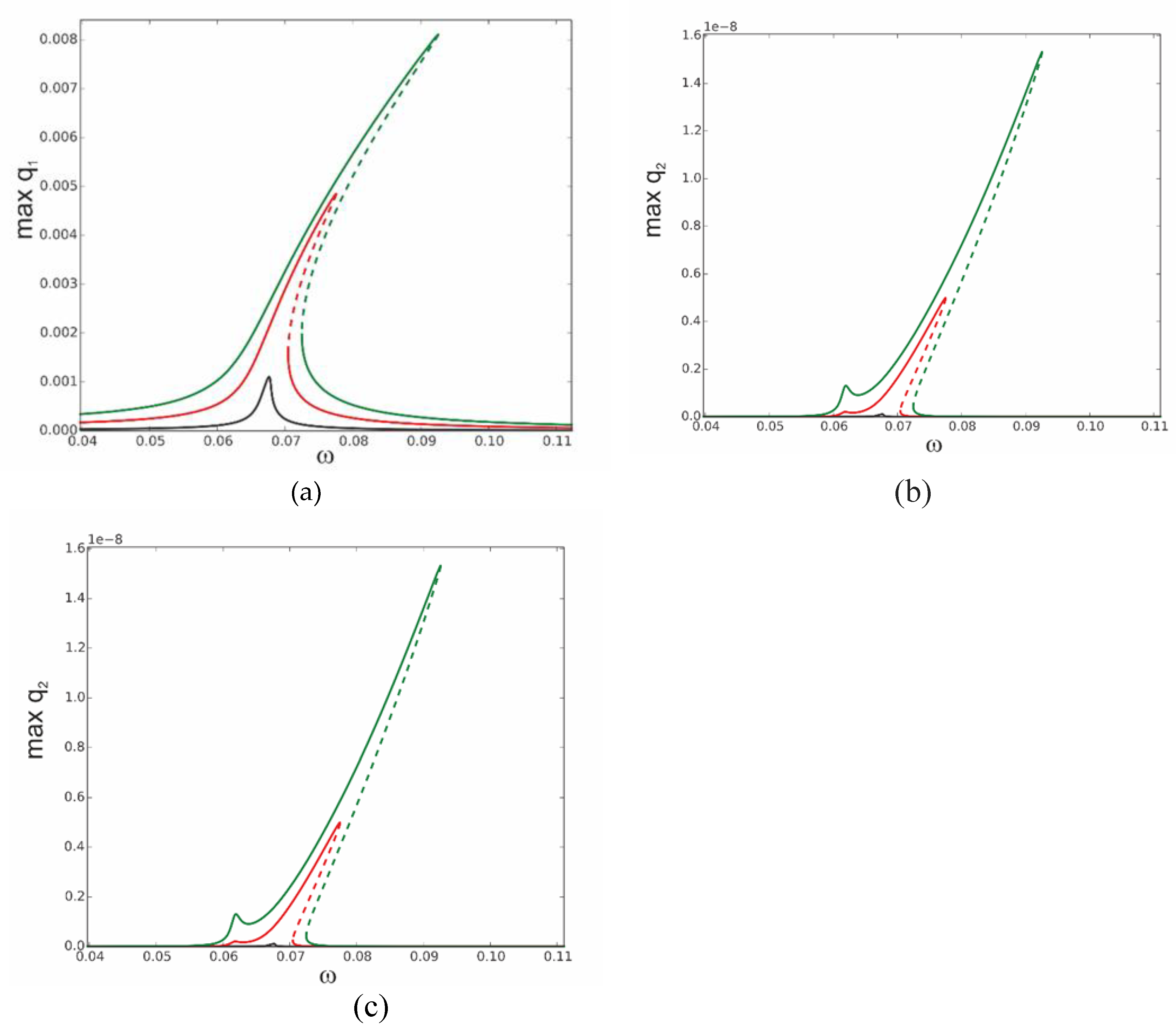
Figure 5.
Resonance curves around the first natural frequency for large mechanical loading, f1 = 0.2×10⁻⁵-black, f1 = 0.1×10⁻⁴-red; ∆T = 0; (a) coordinate q1, (b) zoom of coordinate q1 in vicinity of instable zones, (c) coordinate q2, (d) coordinate q3.
Figure 5.
Resonance curves around the first natural frequency for large mechanical loading, f1 = 0.2×10⁻⁵-black, f1 = 0.1×10⁻⁴-red; ∆T = 0; (a) coordinate q1, (b) zoom of coordinate q1 in vicinity of instable zones, (c) coordinate q2, (d) coordinate q3.
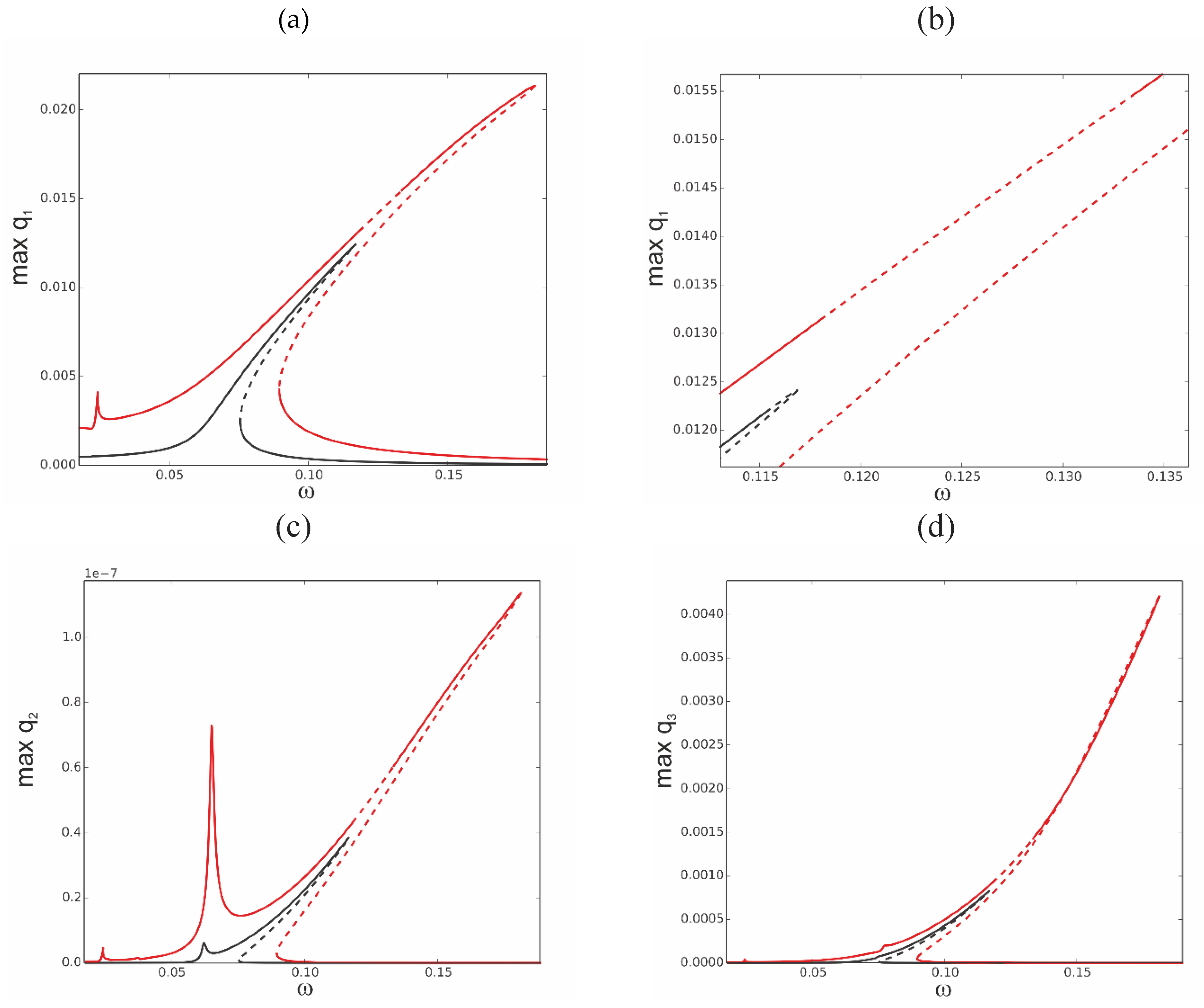
Figure 6.
Resonance curves around the first natural frequency for large mechanical loading, f1 = 0.1×10⁻⁴, f2 = 0, f3 = 0, ∆T = 0; coordinates q1, q2 and q3 with different branches indicated by black, red and blue colours and bifurcation points BP1,BP2.
Figure 6.
Resonance curves around the first natural frequency for large mechanical loading, f1 = 0.1×10⁻⁴, f2 = 0, f3 = 0, ∆T = 0; coordinates q1, q2 and q3 with different branches indicated by black, red and blue colours and bifurcation points BP1,BP2.
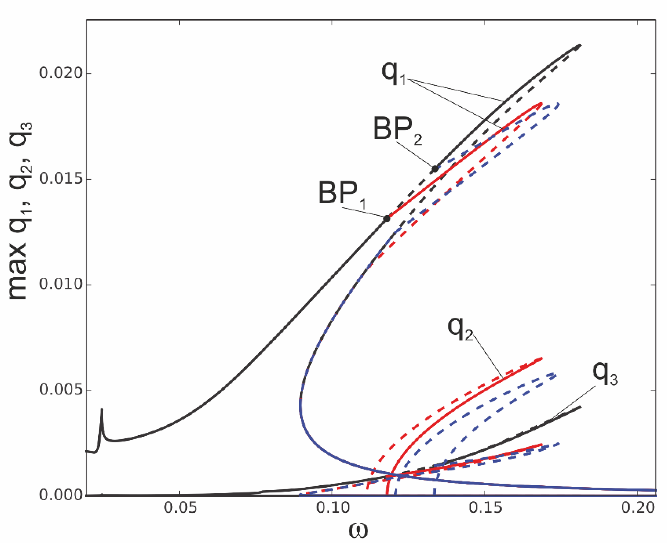
Figure 7.
Resonance curves around the first natural frequency for mechanical loading, f1 = 0.1× 10⁻⁵ and different values of elevated temperature: ΔT = 0 -black, ΔT = 5-.orange, ΔT = 10-pink, ΔT = 15-red, ΔT = 20-brown, ΔT = −10-green, ΔT = −20-blue;.(a) coordinate q1, (b) coordinate q2, (c) coordinate q3.
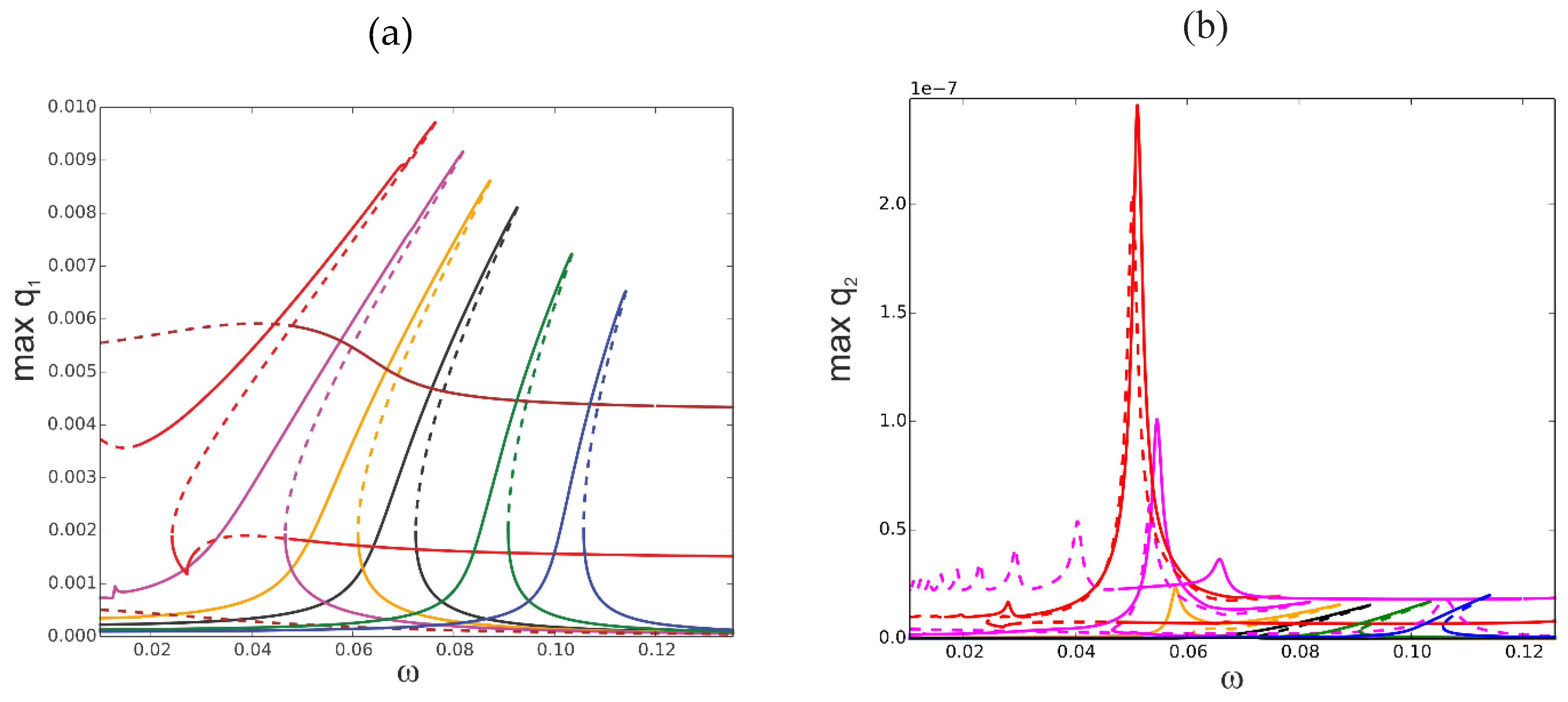
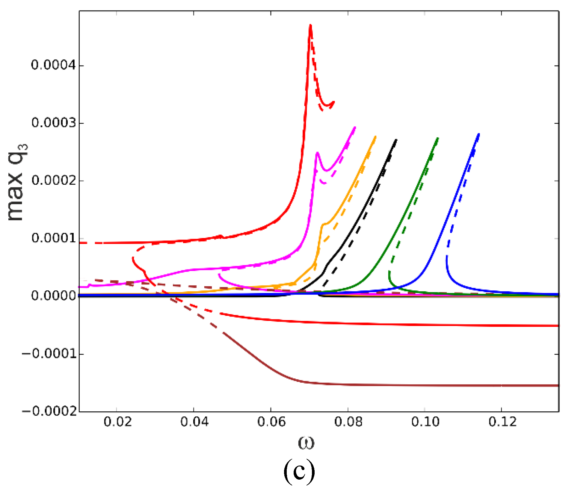
Figure 8.
Resonance curves around the first natural frequency for mechanical loading. Resonance curves around the first natural frequency for mechanical loading,.f1=0.2x10⁻⁵ and different values of elevated temperature: ΔT=0 -black, ΔT =10 -orange, ΔT =15 -red, ΔT =20 -magenta, ΔT =-10 -green, ΔT =-20 -blue, ΔT =-30 -navy blue;.(a) coordinate q1, (b) coordinate q2, (c) coordinate q3.
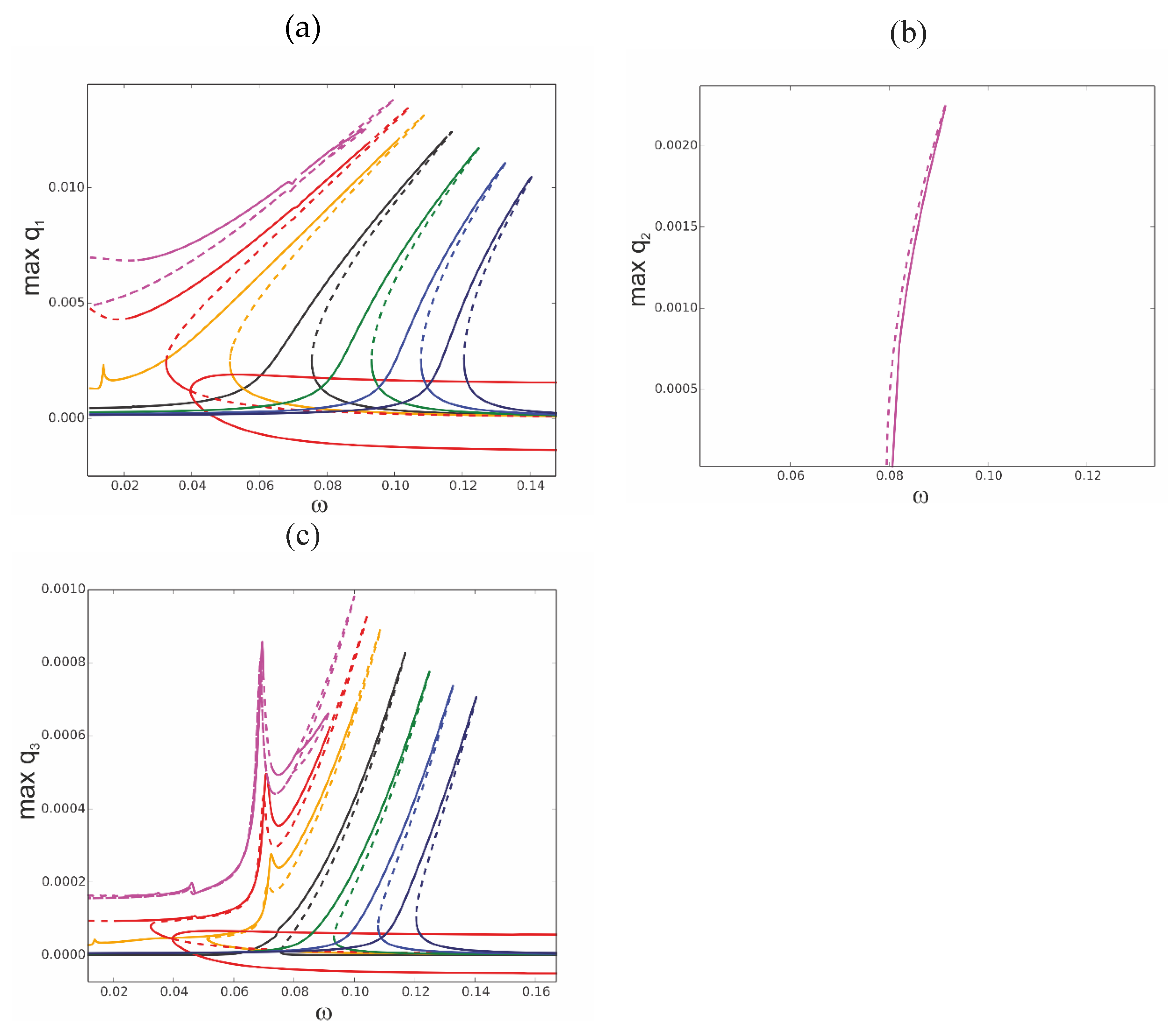
Figure 9.
Bifurcation diagram of beam response against elevated temperature ΔT for fixed mechanical loading f1=0.1 x10⁻⁵ and ω =0.07; BP bifurcation point at ΔT =14.35,.(a) coordinate q1, (b) coordinate q2, (c) coordinate q3.
Figure 9.
Bifurcation diagram of beam response against elevated temperature ΔT for fixed mechanical loading f1=0.1 x10⁻⁵ and ω =0.07; BP bifurcation point at ΔT =14.35,.(a) coordinate q1, (b) coordinate q2, (c) coordinate q3.
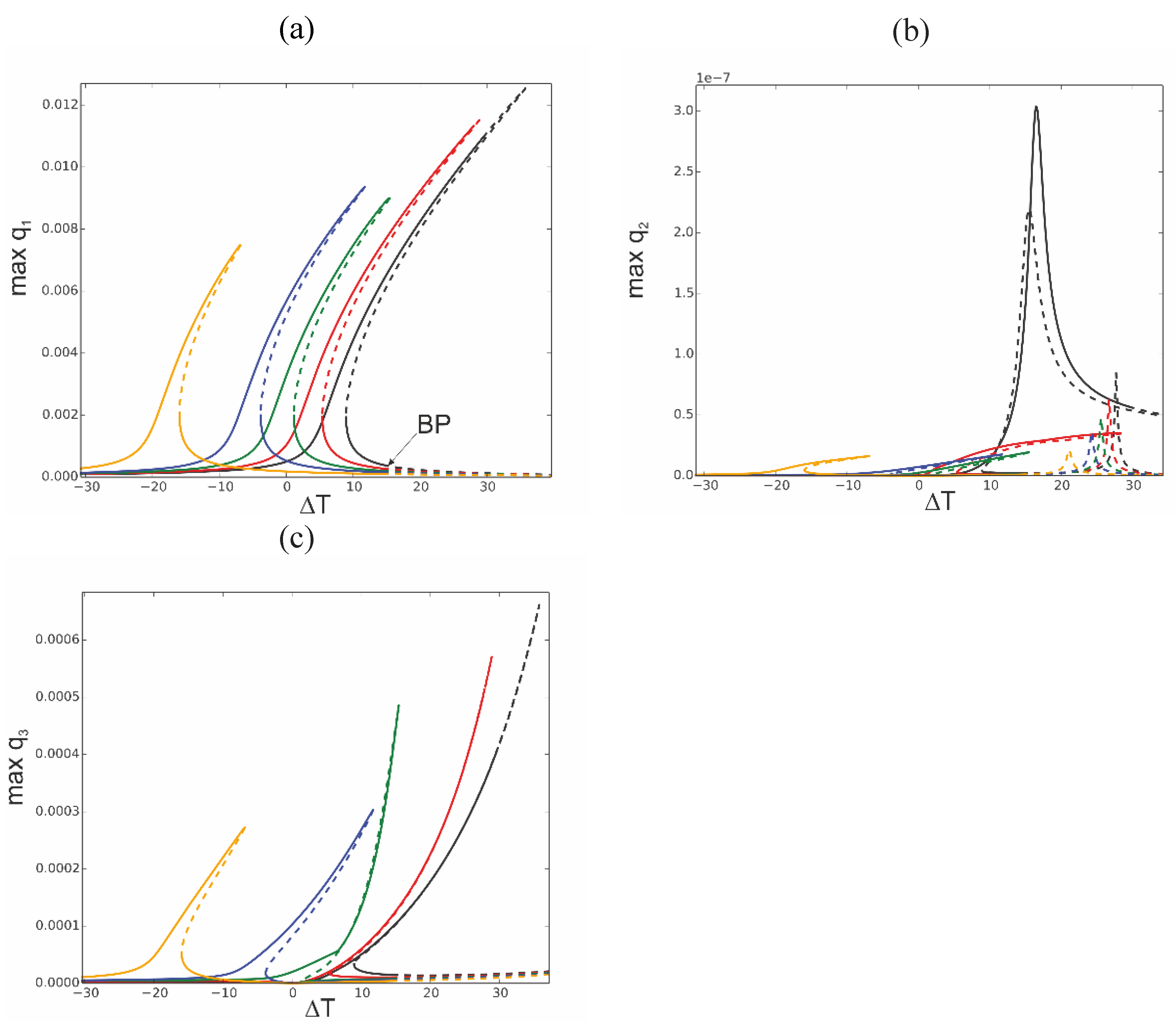
Figure 10.
Bifurcation diagram of beam response against elevated temperature ∆T for fixed mechanical loading f1=0.1 x10⁻⁵ and ω =0.07; BP bifurcation point at ∆T =14.35, post buckling oscillations—red curves, isolated solution—green color;.(a) coordinate q1, (b) coordinate q2, (c) coordinate q3.
Figure 10.
Bifurcation diagram of beam response against elevated temperature ∆T for fixed mechanical loading f1=0.1 x10⁻⁵ and ω =0.07; BP bifurcation point at ∆T =14.35, post buckling oscillations—red curves, isolated solution—green color;.(a) coordinate q1, (b) coordinate q2, (c) coordinate q3.

Figure 11.
Time histories of beam response for selected values of elevated temperature ∆T and mechanical loading, f1=0.1 x10⁻⁵ and ω =0.07; (a) ∆T =14, (b) ∆T=16, (c) ∆T=22, (d) ∆T=35.
Figure 11.
Time histories of beam response for selected values of elevated temperature ∆T and mechanical loading, f1=0.1 x10⁻⁵ and ω =0.07; (a) ∆T =14, (b) ∆T=16, (c) ∆T=22, (d) ∆T=35.
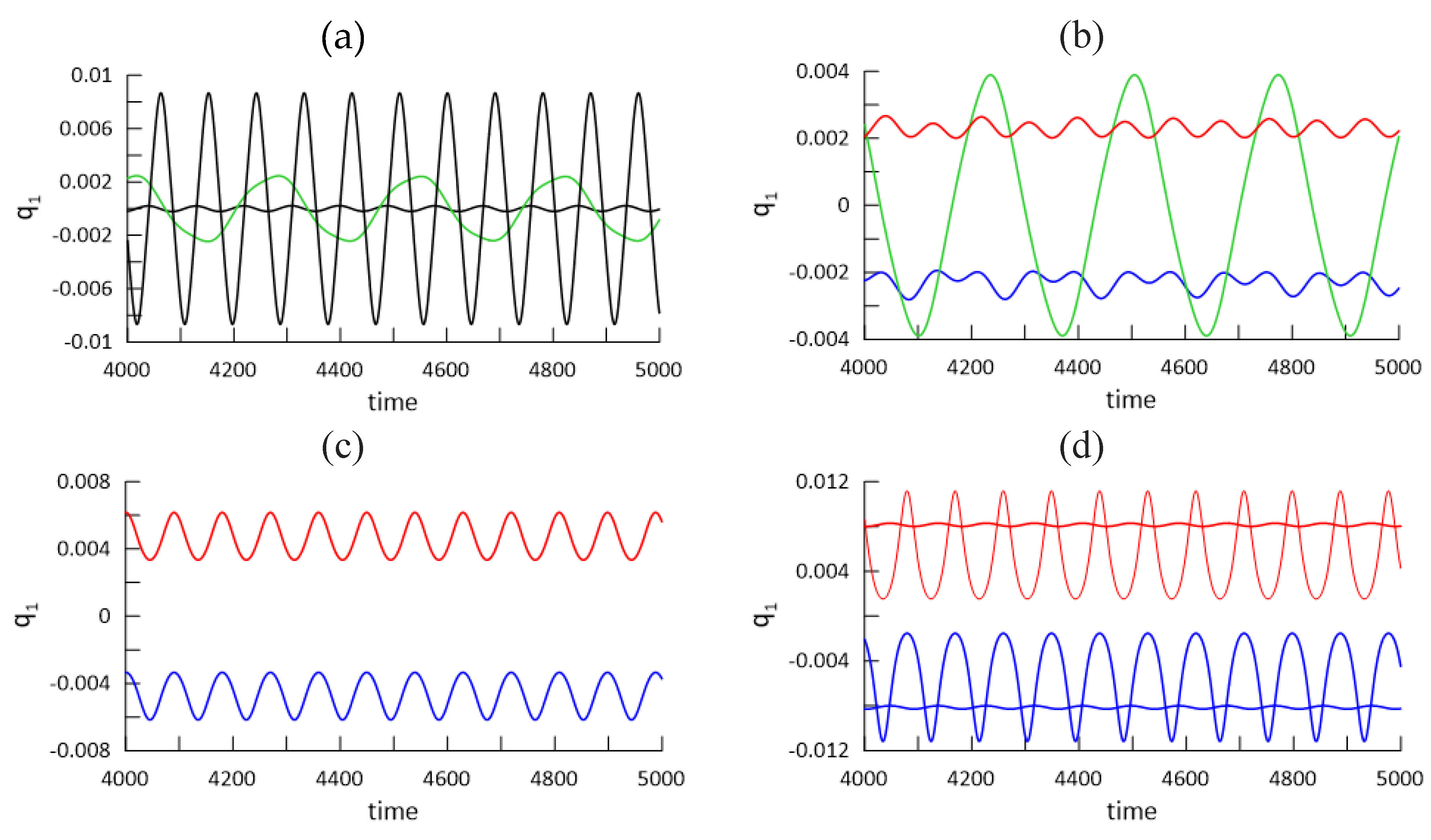
Figure 12.
Resonance curves around the first natural frequency for amplitude of excitation f1=0.1 x10⁻⁵ and different values of distributed temperature: Tup =10, Td =0 -red, Tup =0,.Table 10. -orange, Tup =-10, Td=0 -green, Tup =0, Td =-10 -blue; reference curve: Tup =0,.Table 0. (b) coordinate q2, (c) coordinate q3.
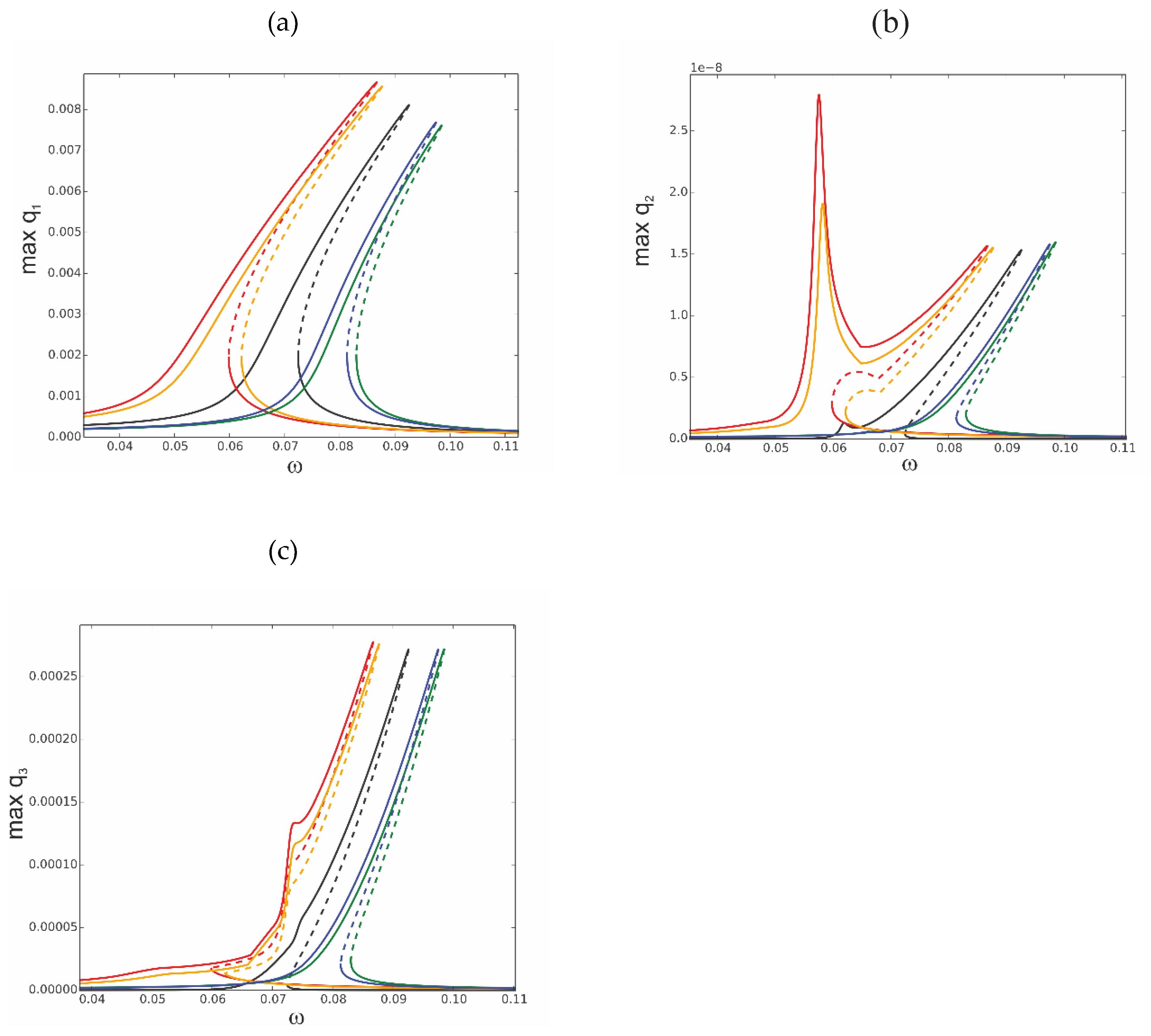
Figure 13.
Resonance curves around the first natural frequency for mechanical loading, 1 x10⁻⁵ and different gradients of linear temperature distribution: Tup =15, Td =-15 -red, Tup =0, Td =10 -black, Tup =-30, Td d=-30 -red, Tup =50, Td =-50 –green,and reference resonance curve for Tup =0, Td =0 -grey; (a) coordinate q1, (b) coordinate q2, (c) coordinate q3.
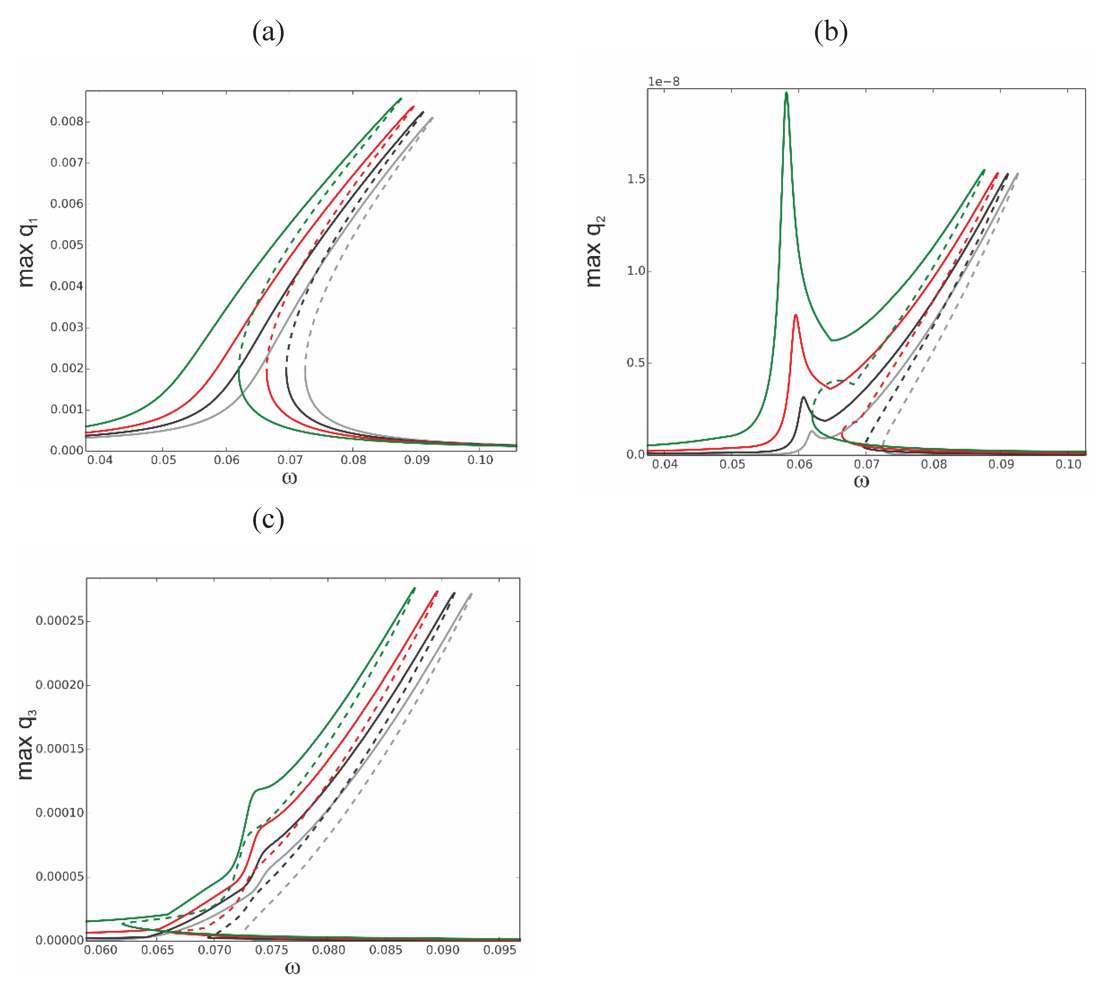
Figure 14.
Bifurcation diagram of coordinate q1 against temperature of the upper beam surface Tup for fixed temperature of bottom surface Td=0, reference response against elevated beam temperature ΔT—grey curve; fixed mechanical loading, f1=0.1x 10⁻⁵ and ω=0.07.
Figure 14.
Bifurcation diagram of coordinate q1 against temperature of the upper beam surface Tup for fixed temperature of bottom surface Td=0, reference response against elevated beam temperature ΔT—grey curve; fixed mechanical loading, f1=0.1x 10⁻⁵ and ω=0.07.
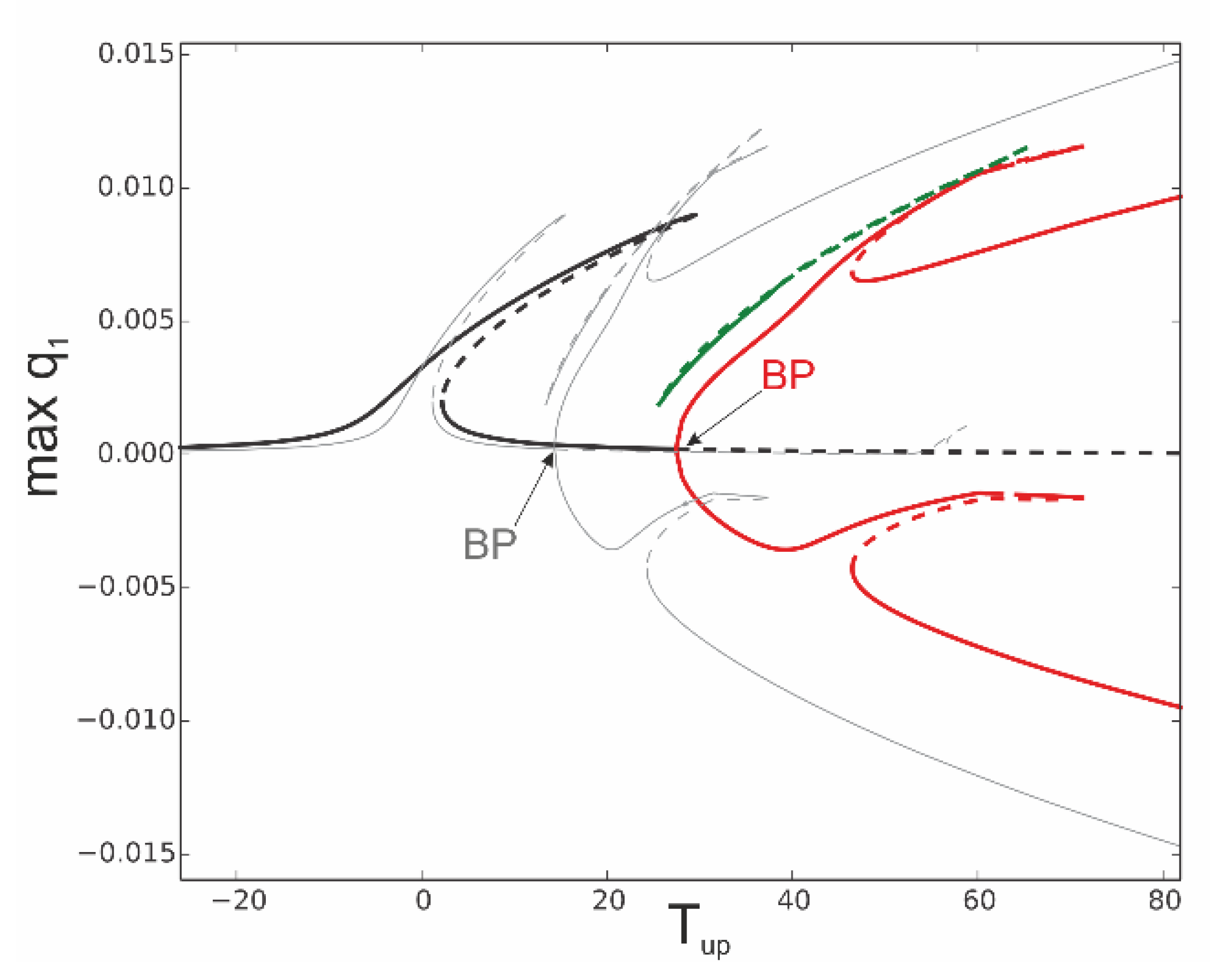
Figure 15.
Resonance curves around the first natural frequency for small mechanical loading, f1 = 0.1 × 10⁻⁶-black, f1 = 0.5 × 10⁻⁶-red, f1 = 0.1 × 10⁻⁵-green, ∆T = 0.
Figure 15.
Resonance curves around the first natural frequency for small mechanical loading, f1 = 0.1 × 10⁻⁶-black, f1 = 0.5 × 10⁻⁶-red, f1 = 0.1 × 10⁻⁵-green, ∆T = 0.
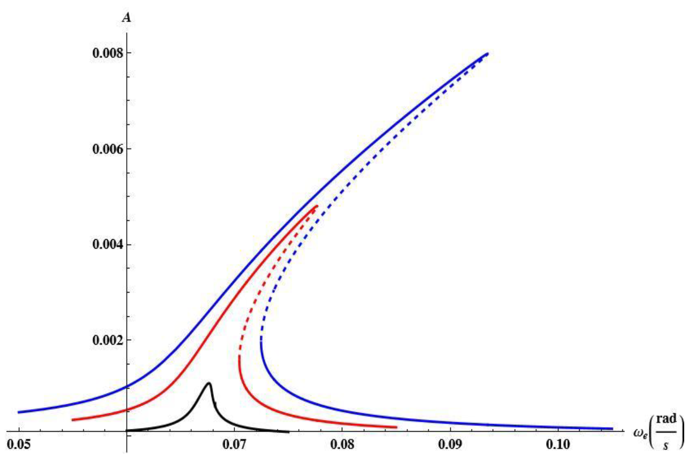
Figure 16.
Resonance curves around the first natural frequency for large mechanical loading, f1 = 0.2×10⁻⁵-black, f1 = 0.1×10⁻⁴-red; f2 = 0, f3 = 0, ∆T = 0.
Figure 16.
Resonance curves around the first natural frequency for large mechanical loading, f1 = 0.2×10⁻⁵-black, f1 = 0.1×10⁻⁴-red; f2 = 0, f3 = 0, ∆T = 0.

Figure 17.
Resonance curves around the first natural frequency for mechanical loading,.
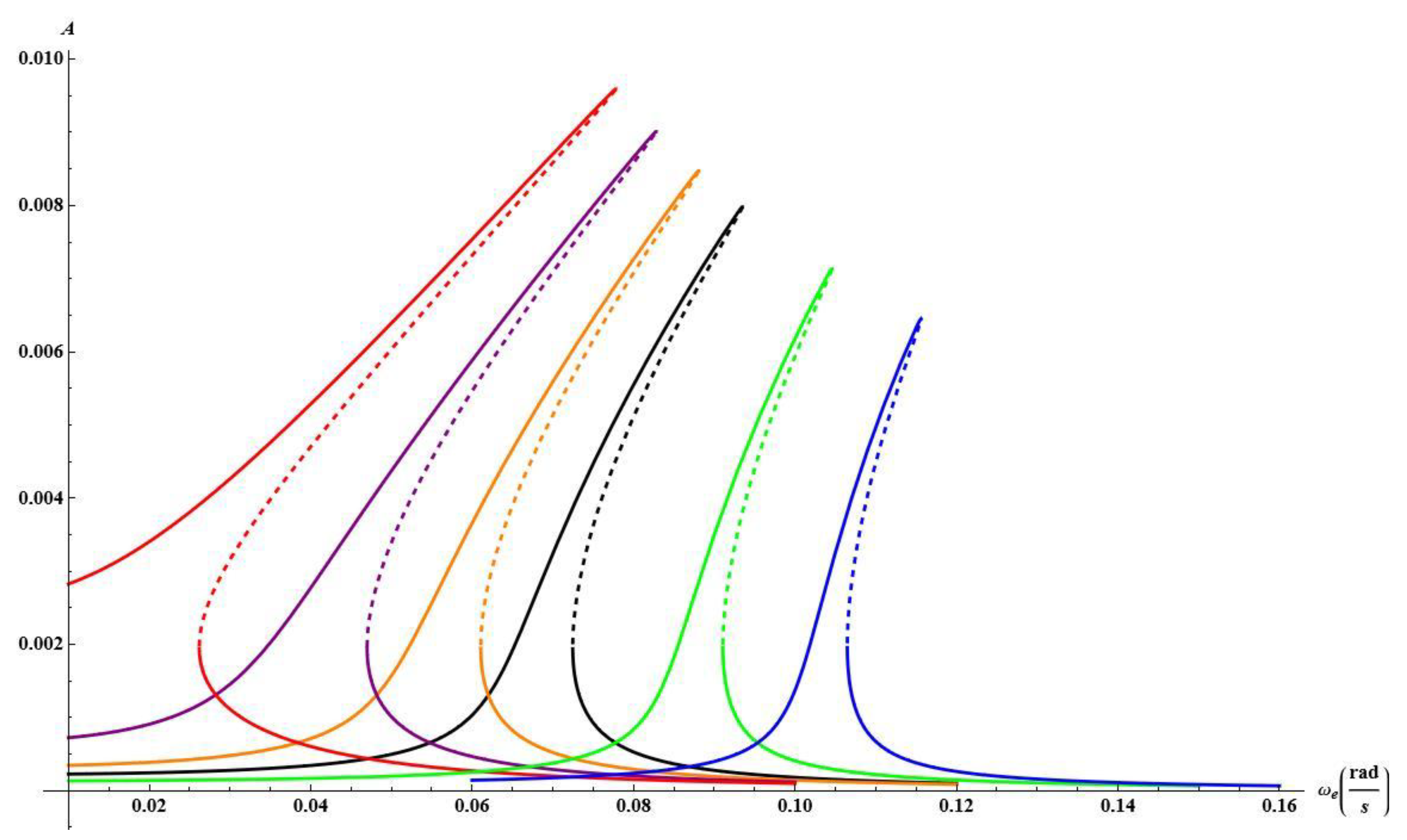
Figure 18.
Resonance curves around the first natural frequency for mechanical loading, f1 = 0.2 ×10⁻⁵ and different values of elevated temperature: ∆T = 0-black, ∆T = 10 orange, ∆T = 15-red, ∆T = 20-magenta,∆T = −10-green, ∆T = −20-blue.
Figure 18.
Resonance curves around the first natural frequency for mechanical loading, f1 = 0.2 ×10⁻⁵ and different values of elevated temperature: ∆T = 0-black, ∆T = 10 orange, ∆T = 15-red, ∆T = 20-magenta,∆T = −10-green, ∆T = −20-blue.
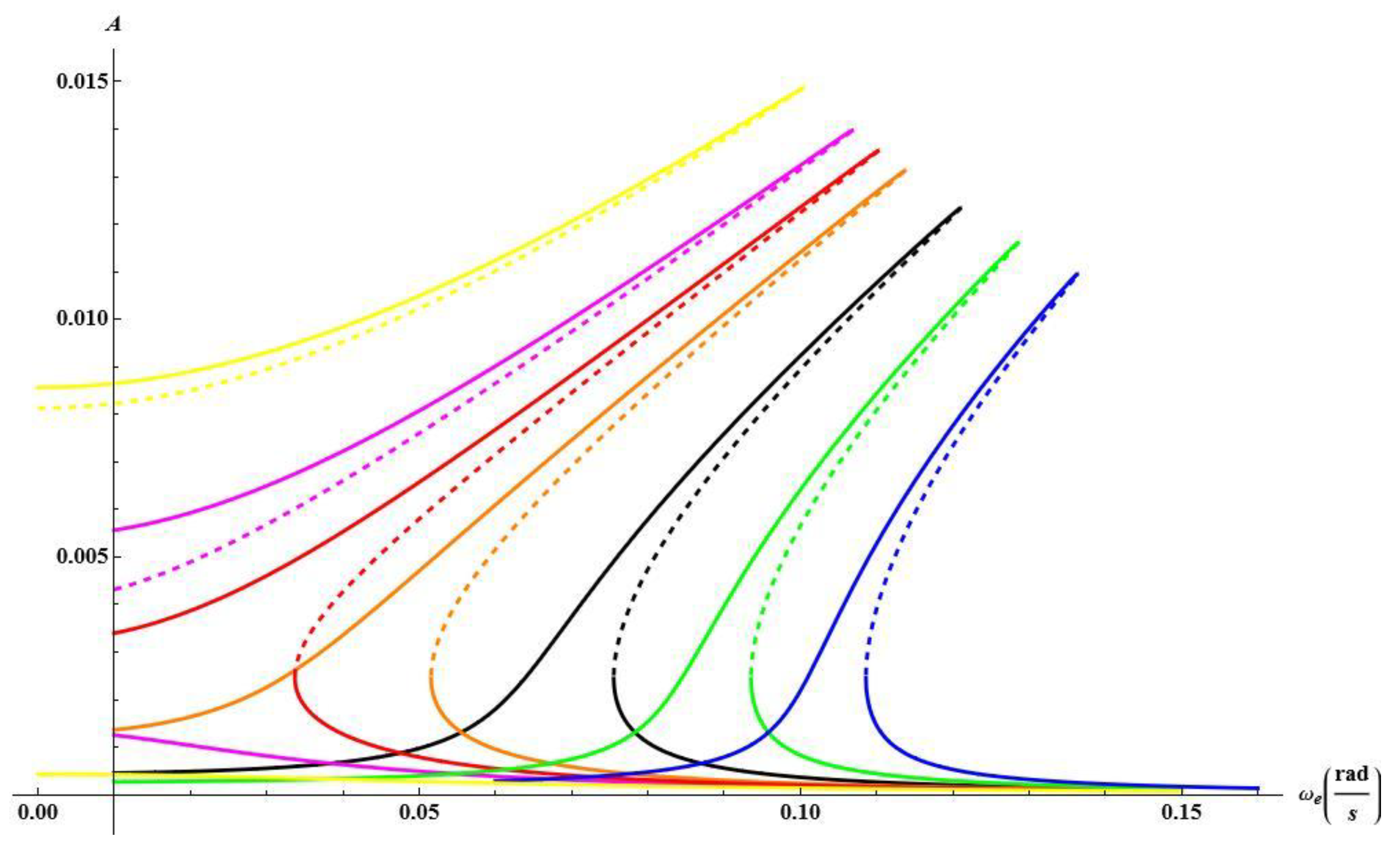
Figure 19.
Bifurcation diagram around beam response against elevated temperature ∆T.
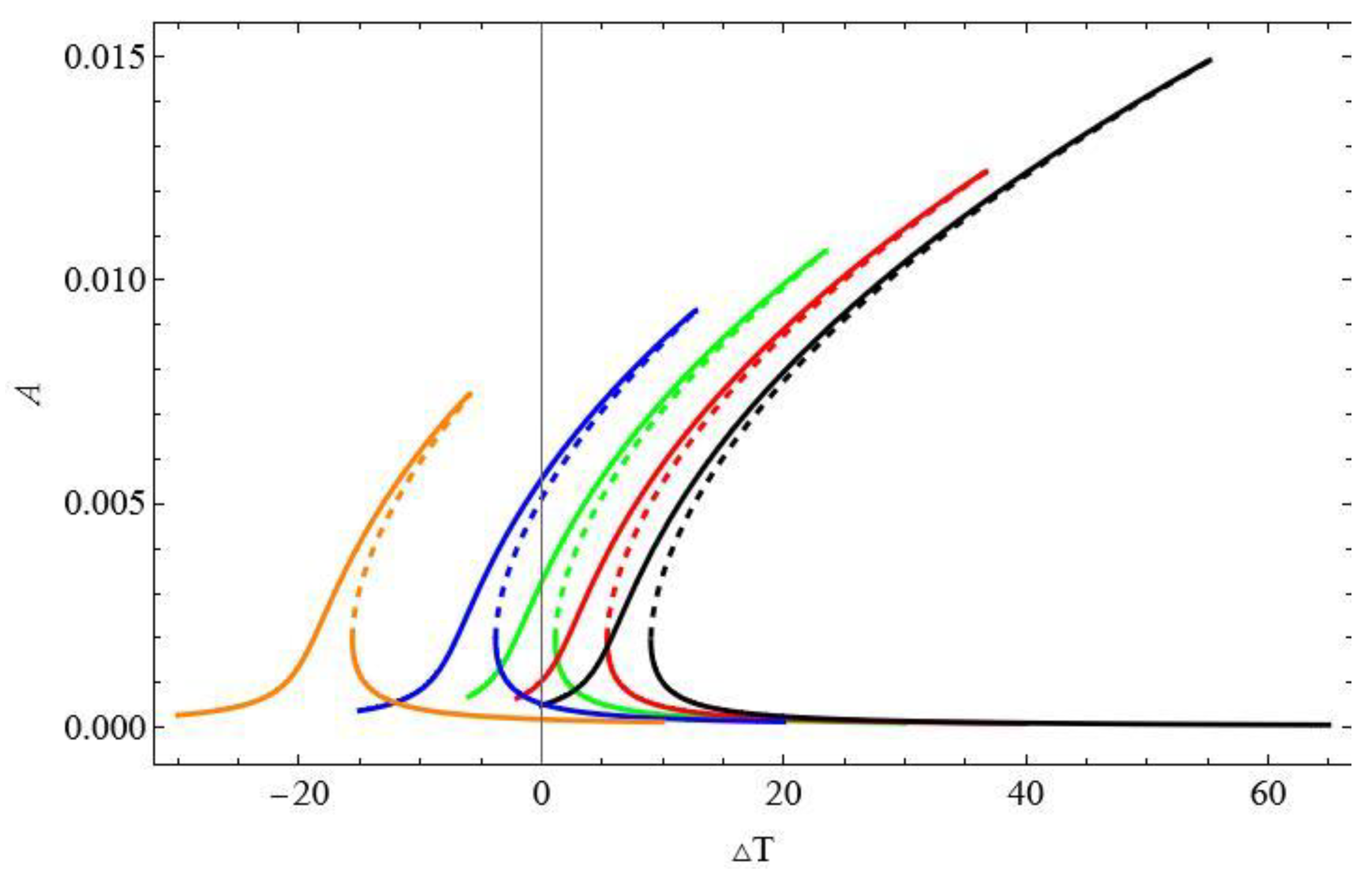

Table 1.
Natural frequencies of the beam according to finite element model and the Timoshenko beam theory for the homogenized beam.
Table 1.
Natural frequencies of the beam according to finite element model and the Timoshenko beam theory for the homogenized beam.
| No | Reduced Model | Finite Element Model | Differences % |
|---|---|---|---|
| 1 | 108.77 | 117.39 | 7.3 |
| 2 | 299.53 | 323.30 | 7.35 |
| 3 | 586.42 | 633.20 | 7.38 |
Disclaimer/Publisher’s Note: The statements, opinions and data contained in all publications are solely those of the individual author(s) and contributor(s) and not of MDPI and/or the editor(s). MDPI and/or the editor(s) disclaim responsibility for any injury to people or property resulting from any ideas, methods, instructions or products referred to in the content. |
© 2025 by the authors. Licensee MDPI, Basel, Switzerland. This article is an open access article distributed under the terms and conditions of the Creative Commons Attribution (CC BY) license (http://creativecommons.org/licenses/by/4.0/).
Copyright: This open access article is published under a Creative Commons CC BY 4.0 license, which permit the free download, distribution, and reuse, provided that the author and preprint are cited in any reuse.


