Submitted:
09 October 2025
Posted:
10 October 2025
You are already at the latest version
Abstract
This work presents a comprehensive framework for the multiscale characterization of advanced composite structures, focusing on Mindlin plates and Timoshenko beams with periodic microstructures. Using a second-order two-scale (SOTS) method, we uniformly derive asymptotic expansions for deflection and rotation to formulate effective homogenized models. The developed finite element procedures combine techniques to overcome shear locking, enabling efficient and accurate structural application. Numerical simulations verified the convergence of the model and demonstrated its superiority in capturing the rapid oscillation of local stress distribution, an important aspect for the design of reliable composites. By varying the thickness parameter, our model is shown to connect thin and thick theories for composite beam and plate problems. It thus provides a practical tool for the design and analysis of tailored composite structures, contributing to the development of innovative materials.
Keywords:
multiscale characterization
; second-order two-scale (SOTS) analysis
; finite element method
; structural application
; Mindlin plate
; Timoshenko beam
1. Introduction
The transition between precise material characterization and reliable structural application is a core challenge in the development of advanced composite materials. To achieve this goal, we need to establish a unified model that can accurately describe the complex mechanical behavior of composite materials under different structural forms. In previous works, the composite Kirchhoff plate and Euler beam theories have been widely applied in the thin structures [1,2]. However, due to the assumption that cross-section after deformation is perpendicular to the neutral axis and the lateral shear effect is ignored, the deviation is relatively large when simulating moderate thick composite materials. In this case, it is necessary to consider the composite Mindlin plate [3] and Timoshenko beam models, which can recover the Kirchhoff plate and Euler beam models as the thickness decreases. It has provided convenience for the efficient characterization and simulation of the effectiveness of modern composite materials.
Modern composite materials, composed of two or more different materials, such as ultra-high temperature ceramic composite plate reinforced with superalloys, carbon fiber reinforced epoxy resin composite plate [4,5], are widely used in aerospace, automotive and other high-performance engineering fields. These materials are valued for their outstanding rigidity and superior corrosion resistance, demonstrating remarkable adaptability to specialized application requirements. From a mathematical point of view, solving these equations requires dealing with rapidly varying coefficients. Due to the large scale of calculations, the conventional method incurs significant computational costs. Traditional formulations of plate and beam theory often fall short in capturing the complex behavior of structures with multiple length scales. A practical method proposed to simplify these calculations is the homogenization method [6]. By applying multi-scale expansion, homogenized solutions and cell functions can be obtained to describe both macroscopic and microscopic properties. This method improves the computational efficiency by homogenizing the microstructure features into effective macroscopic parameters, avoiding the expensive discretization at the microscale. Furthermore, the oscillating behavior of solutions can be effectively corrected. Based on the establishment of mathematical theories about the homogenization method [7,8,9], the multi-scale finite element method (MsFEM) [10], the heterogeneous multi-scale method (HMM) [11,12], and the variational multi-scale method (VMM) have been proposed and developed. Noticing that only first-order asymptotic analysis was established, Cui and Cao considered second-order asymptotic analysis [13]. Applying this method to simulate the deformation of composite materials is more accurate, and corresponding finite element algorithms have been established [14,15,16]. This SOTS asymptotic analysis is now applied to a variety of problems, such as thermoelasticity [17,18,19], elasticity problems [20,21], and so on.
However, significant technical difficulties arise in directly applying this asymptotic expansion to the classical theories of thin structures, namely the Kirchhoff plate and Euler beam problems. In the process of asymptotic expansion and analysis, these problems are described by fourth-order partial differential equations. After conducting an asymptotic analysis of models, it has been demonstrated that three-dimensional composite plate can be simplified to two-dimensional uniform Kirchhoff plate as the thickness h and approach zero [22]. Lewiński and Józef used the homogenization method and two-scale expansion method to solve the composite Mindlin plate problem in two dimensions [23]. Zhu and Cui provided a new Second-Order Two-Scale(SOTS) method for the Mindlin plate theory, and the laminated homogenization plate was analyzed [24]. Wang and Cui considered the bending behaviors of composite plate with 3-D periodic configuration and established a SOTS method, proving the approximation property of the solution by energy norm estimation [25]. Huang et al. established a two-scale asymptotic homogenization method for periodic composite Kirchhoff plate and Euler beam [26,27]. Numerical comparisons demonstrated that the current method is both physically acceptable and highly accurate.
As is known that directly establishing the SOTS asymptotic model for the fourth-order Kirchhoff plate and Euler beam directly is not easy, so it is reasonable to alternatively perform this high-order expansion on the second-order equations for Mindlin plate and Timoshenko beam first, and then proceed to consider approximating the corresponding composite Kirchhoff plate and Euler beam by letting the thickness h approach zero. We believe that this two-step strategy can not only obtain the asymptotic behavior of the Mindlin plate and Timoshenko beam, but also capture the local variations of the corresponding Kirchhoff plate and Euler beam. This is the principal idea and the main interest of our work, which are not seen elsewhere to the best of our knowledge. It should also be noted that when h is very small, the zero shear strain constraint leads to the shear locking [28,29,30], and we will discuss how to avoid this phenomenon in the asymptotic computing.
For these purposes mentioned above, the paper is structured as follows: The governing equations for the composite Mindlin plate and Timoshenko beam are presented in Section 2, and the corresponding SOTS asymptotic expansions are derived in Section 3. The finite element algorithm and symbol definitions for the second-order asymptotic plate and beam models are presented in Section 4. Several numerical examples of the SOTS asymptotic expansions for the Mindlin plate and the Timoshenko beam are given. The approaching behavior for the thick-thin theory of the plate and beam for the stationary problem are shown in Section 5. The conclusion remarks are given in Section 6. For simplicity, the Einstein summation convention is used, where the repeated subscript implies summation.
2. Governing Equations
The configuration of the composite plate with thickness h is typically shown in Figure 1(a). Different constituent materials are periodically distributed in the and directions and are homogeneous in the thickness direction. The normalized periodic cell is depicted in Figure 1(b).
Define the two-dimensional middle plane as and the unit cell as Y. With the micro and macro coordinates being and , respectively, a small parameter is defined to relate these variables as
where is floor operator.
The governing equations for the composite Mindlin plate can be formulated as
where and are the shear stresses, and are the bending moments, is the torsional moment, and represents the external load on the plate.
The shear stress and can be expressed by
where is the deflection, and are the rotations of the cross section, is the Young’s modulus, is the shear correction factor, and is the Poisson’s ratio. and are periodic due to the configuration and can be expressed as
where and are periodic functions defined in Y. The constitutive relation between bending moment and curvature is given by
For simplicity, clamped boundary conditions are imposed on and the Mindlin plate problem is given as
where is defined by
and is the shear modulus, related to and through .
The Timoshenko beam problem is equivalent to the dimensional reduction of the plate problem (6). Therefore, the composite Timoshenko beam problem takes the following form:
where is the one-dimensional deflection, is the rotation, A is the sectional area, given by with b being the width, and is the external load on the beam.
3. The SOTS Asymptotic Analysis
First, we perform the SOTS asymptotic analysis for the composite Mindlin plate problems (6). Following the standard procedure, the deflection , rotation can be expanded as
with the homogenized solutions , , appended by the first-order correctors , and the second-order terms , . Transforming the partial derivatives as
substituting Eqs. (9) into governing equations (6), and equating the power coefficients of , the equations for the first three expansion terms are obtained as follows:
From (11), the first-order correctors and are defined as
where the first-order cell functions and are solutions to the following boundary value problems:
Next, taking the integral average over the unit cell Y in (12), and using the newly defined expressions for and from (13), the homogenized Mindlin plate problem can be defined as follows:
where the homogenized coefficients and , and the homogenized load are given by
respectively, where is the measure of the domain Y.
A high-order expansion is necessary to capture the local oscillation behavior of deflection and rotation. By substituting the homogenized equation (16) and the first-order expansion (13) into (12), the second-order correctors and have the following expressions:
where the second-order cell functions , , , and are solutions to the following cell problems:
Next, we move to the Timoshenko beam problem (8). Based on the results from the Mindlin plate problem, the expansions of and can be directly obtained as
where the first-order cell functions and respectively satisfy the following problems:
The homogenized solutions and are obtained from
where the homogenized coefficients and , and from (22) are respectively defined by
The second-order cell functions , , , and are solutions to the problems:
4. Multi-Scale Finite Element Algorithm
According to the expansions of the deflections and rotations, we can establish the finite element(FE) algorithms for the plate and beam problems. The multiscale computational flowchart for Mindlin plate is shown in Figure 2. Two kinds of meshes are generated before the multiscale computations: cell mesh and homogenized mesh. All the cell functions are solved on the cell mesh, and the homogenized solutions are obtained on the homogenized mesh. First, let us define the first-order and second-order approximate solutions as follows:
with the homogenized shear stresses and the first-order and second-order approximate shear stresses and , respectively, given by
The FE procedures for plate problem are illustrated as follows:
1. Preprocessing: Set the material coefficients and , define the periodic cell Y and the homogenized domain , perform the spatial discretization and generate the computational meshes. To illustrate the efficiency of the SOTS model proposed in this paper, we also partition a sufficiently refined mesh and conduct the classical computations for and as the reference solution for comparison.
2. Computations of the cell functions:
(2) Calculate the homogenized coefficients , , and from Eq (17).
(3) Solve the second-order cell functions , , , and .
3. Computations of the homogenized solutions and .
4. Assembly of the first-order and second-order multiscale approximations , , , and from Eq (24) in an incremental way.
5. Postprocessing: Compute the first-order and second-order multiscale approximate shear stresses: , , and based on Eq (25).
As is well known, the effects of shear deformations become negligible as the thickness decreases. To address this, consistent interpolation element (CIE) is employed to solve the plate problem.
To evaluate the accuracy of the proposed asymptotic model, the relative errors are defined by
where , , and .
5. Numerical Examples
5.1. Multi-Scale Approximation for Plate Problem
The SOTS asymptotic expansion method is applied to Mindlin plates made of various composite materials. Several numerical examples are provided to test the accuracy of the proposed algorithm.
5.1.1. Composite Mindlin Plate
Consider a square plate of length with thickness m, clamped on all sides and subjected to a uniform load kN. The macro region and representative cell are shown in Figure 3 (a) and (b), respectively. Let material be carbon steel with and , and material be low-density polyethylene(LDPE) with and . The shear correction factor is adopted for both materials. is chosen as , . The mesh information for the classical FE computations and SOTS approximation is listed in Table 1. It is evident that the classical computations take a significant amount of computational time while the proposed SOTS asymptotic method requires calculations only on a single cell and a homogenization domain with much less CPU time and also memory requirement. The relative -errors of the approximation solutions are displayed in Table 2, which can be seen that the errors decreases as becomes small.
The convergence curves of deflection and rotations with respect to are presented in Figure 4. It is observed that the convergence orders for and are approximately and , respectively. Due to all the cell functions and homogenized solutions have to be mapped into the fine meshes with different . The interpolations errors between the cell mesh, homogenized mesh and the fine meshes as well as the numerical differential errors for computing the high-order derivatives of the homogenized solutions influence the relative errors computations, which to some extent conceal the convergence order of the asymptotic models.
Figure 5 and Figure 6 show the computed deflection and rotations when . It is indicated that adding the second-order approximations provides a better approximation of due to the pronounced changes in deflection w. The second-order correctors and show a slight improvement over the first-order correctors and , because the changes in rotation and are less obvious. Overall, the SOTS asymptotic expansions offer a more accurate representation of oscillatory behavior compared to the first-order solutions.
The approximation of the shear stresses can be obtained when , which is shown in Figure 7. It can be observed that the oscillations are more remarkable for the stress distributions than the displacement field (Figure 7 (a) and (e)), the homogenized solutions in Figure 7 (b) and (f) only give the macroscopic behavior and the first-order solutions in Figure 7 (c) and (g) are not capable of capturing the peak of the stress within the constituent material LDPE. Therefore, the second-order correctors are necessary to be defined and appended in the asymptotic expansions to give the satisfactory distributions, which are shown in Figure 7 (d) and (h).
Figure 8 illustrates the approximations of shear stresses along the diagonal line, and it is evident that incorporating second-order correctors provides a more accurate characterization of oscillations compared to both homogenized solutions and first-order approximations.
5.1.2. Convergence for Kirchhoff Plate
Next, we check if the asymptotic model is also effective to describe the behavior of the Kirchhoff plate. Consider also a clamped square plate with a uniform load kN. The material parameter in and is the same as in [24]. For the macroscopic domain and each microscopic cell, divide the domain into 80 × 80 squares and 50 triangles for calculations.
To quantify the convergence behavior of the composite plate, , , and are computed using the discrete Kirchhoff theory. The computed relative -errors are given by:
Let be 0.2, 0.1, and 0.035, respectively. Perform traditional FE computation for the Kirchhoff plate and compare these with asymptotic solutions. Although the plate model exhibits no significant shear locking, implementation of the CIE method is still required to prevent potential locking effects. Table 3, Table 4, and Table 5 present the relative -errors for different . It is observed that and of the Mindlin plate converge to and , while approaches as h decreases. The deflection can be approximated by when h is not small, whereas provides a more accurate approximation when h decreases. Due to the relatively smooth variation in , shows only a limited improvement in accuracy compared with and . and are best approximated by appending and , which can also be shown in Figure 9 and Figure 10.
A comparison with the numerical example in [24] is performed to validate the rationality of the approach proposed in this paper. The unit cell has a height of 1 cm and in-plane dimensions of Y, measuring 0.3 × 0.3 cm2, with a square inclusion at its center. Under the same conditions as in Example 1: Free Vibration of a CCCC Single-Layer Periodic Plate, the homogenized stiffness matrix can be
which is closely matches the homogenized stiffness matrix given in [24] as follows:
5.2. Multi-Scale Approximation for Beam Problem
The SOTS method is also utilized to analyze the composite Timoshenko beam.
5.2.1. Composite Timoshenko Beam
Consider a composite beam of unit length with width and height , which is clamped at both ends and subjected to a uniform load . The macro and cell domains are shown in Figure 11 (a) and (b), where () is occupied by the material (). Choose and for the plumbum () in , and and for the alloy steel () in . The macroscopic domain is discretized into 100 finite elements for computation. Let be , . The computed relative -errors are shown in Table 6.
It is shown that the SOTS computation also offers improved precision for approximating both and with less computational effort compared to the general FE method.
The asymptotic approximations for , , and are presented in Figure 12, with local detail graphs within. Compared to , and are gradually closer to and for and . As shown in the figures, the approximation for is more effective compared to with more details captured.
The converging behaviors of the deflection and the rotation with respect to are shown in Figure 13. It can be observed from the figure that the convergence rates for the and are approximately , whereas the convergence order of the homogenized result is approximately .
5.2.2. Convergence for Euler Beam
Choose . As the thickness h decreases, the beam model requires finer mesh discretization. In the macroscopic domain, the domain is divided into 400 mesh elements for calculations, and other parameters are selected similarly to those in Section 5.2.1. Define and as the deflection and rotation of the Euler beam obtained by the general FE method. The relative -errors and are defined similarly to (27).
Compare the solutions of the numerical method with the solutions and of the Euler beam using the general finite element method. Since the rotation of the Timoshenko beam remains close to the rotation for , , and , while the deflection of the Timoshenko beam approximates more accurately when h is small, as shown in Figure 14 (a)-(f). It is shown that approximating the deflection by appending the second-order corrector is more effective than using the first-order corrector and the homogenized solution , when h is small as and . The microscopic homogenized coefficients used to obtain the homogenized Euler beam are displayed as follows:
The relative -errors of the homogenized Euler beam when approximating the composite Euler beam are displayed in Table 7. As gradually decreases, the relative errors are reduced, and approximations of both deflection and rotation improve.
Additionally, the rotation is better approximated by adding the second-order corrector than using the homogenized solution or appending the first-order corrector for different values of h. This is detailed in Table 8, Table 9, and Table 10. As h decreases from 0.1 m to 0.02 m, the composite Timoshenko beam gradually approximates the composite Euler beam more closely.
When the thickness h reaches a minimum of 0.02 m, no significant shear locking phenomenon is observed. However, when h is less than 0.001 m, pronounced shear locking occurs, necessitating the application of RIE method to address this numerical issue.
6. Conclusions
A two-scale asymptotic framework is established for composite Mindlin plates and Timoshenko beams, demonstrating that the second-order correctors are crucial for accurately capturing stress oscillations at material interfaces. When h decreases, the asymptotic model developed can effectively approximate the Kirchhoff plate and Euler beam with composite configurations, respectively, providing an alternative way to simulate complicated thin plate and beam structures. The RIE and CIE are employed in the finite element computations of the homogenization models to mitigate shear locking, which can give an accurate description of the displacement and stress distributions of the plates and beams.
Most importantly, the proposed method offers significant potential for future work. It can be directly extended to model sustainable composites with valorised manufacturability. This establishes our asymptotic framework as a general and computationally efficient approach for predicting the multi-physical response of next-generation composite plates and beams, thereby contributing to the development of tailored material systems aligned with the goals of modern industrial applications.
Author Contributions
Conceptualization, M.Z., Q.M.; methodology, M.Z. and Q.M.; software, M.Z. and Q.T.; validation, M.Z., Q.M. and Q.T.; formal analysis, M.Z. and Q.M.; investigation, M.Z.; data curation, M.Z. and Q.T.; writing—original draft preparation, M.Z.; writing—review and editing, M.Z., Q.M.; visualization, M.Z.; supervision, Q.M. ; project administration, Q.T.; funding acquisition, Q.M. and Q.T. All authors have read and agreed to the published version of the manuscript.
Funding
This research was funded by the National Key R&D Program of China (No.2024YFA1012803), National Natural Science Foundation of China (U24B2073) and the Natural Science Foundation of Sichuan Province (Grant No.2024NSFSC0438).
Data Availability Statement
The data presented in this study are available on request from the corresponding author. The data are not publicly available due to privacy concerns.
Acknowledgments
The authors gratefully acknowledge the reviewers’ constructive suggestions and insightful comments that have helped strengthen this research.
Conflicts of Interest
The authors declare no conflicts of interest.
References
- Jangravi, S.; Masjedi, P.K.; Reali, A. Equilibrium-based 3D stress recovery of laminated anisotropic composite plates via isogeometric analysis. Compos. Struct. 2025, 365, 119144. [Google Scholar] [CrossRef]
- Patton, A.; Antolín, P.; Dufour, J.E.; Kiendl, J.; Reali, A. Accurate equilibrium-based interlaminar stress recovery for isogeometric laminated composite Kirchhoff plates. Compos. Struct. 2021, 256, 112976. [Google Scholar] [CrossRef]
- Wan, D.; Hu, D.; Natarajan, S. A linear smoothed quadratic finite element for the analysis of laminated composite Reissner-Mindlin plates. Compos. Struct. 2017, 180, 395–411. [Google Scholar] [CrossRef]
- Lee, C.Y.; Yu, W.B. Homogenization and dimensional reduction of composite plates with in-plane heterogeneity. Int. J. Solids Struct. 2011, 48(1), 1474–1484. [Google Scholar] [CrossRef]
- Huang, Z.W.; Xing, Y.F.; Gao, Y.H. A new method of stiffness prediction for composite plate structures with in-plane periodicity. Compos. Struct. 2021, 280, 114850. [Google Scholar] [CrossRef]
- Cioranescu, D.; Donato, P. An Introduction to Homogenization; Oxford University Press: New York, USA, 1999. [Google Scholar]
- Bensoussan, A.; Lions, J.L.; Papanicolaou, G. Asymptotic Analysis for Periodic Structures; North-Holland: Amsterdam, Netherlands, 1978. [Google Scholar]
- Lions, J.L. Some Methods in the Mathematical Analysis of Systems and Their Control; Science Press, Gordon and Breach Science Publishers: Beijing, China, 1981. [Google Scholar]
- Jikov, V.V.; Kozlov, S.M.; Oleinik, O.A. Homogenization of Differential Operators and Integral Functional; Springer-Verlag: Berlin-Heidelberg, Germany, 1994. [Google Scholar]
- Hou, T.Y.; Wu, X.H. A multiscale finite element method for elliptic problems in composite materials and porous media. J. Comput. Phys. 1997, 134, 169–189. [Google Scholar] [CrossRef]
- Abdulle, A.; E, W.N.; Engquist, B.; Vanden-Eijnden, E. The heterogeneous multiscale method. Acta Numer. 2012, 21, 1–87. [Google Scholar] [CrossRef]
- E, W.N. Principles of Multiscale Modeling; Science Press: Beijing, China, 2012. [Google Scholar]
- Cui, J.Z.; Cao, L.Q. Finite element method based on two-scale asymptotic analysis. Math. Numer. Sin. 1998, 20(2), 89–102. [Google Scholar]
- Cao, L.Q.; Cui, J.Z. Asymptotic expansions and numerical algorithms of eigenvalues and eigenfunctions of the Dirichlet problems for second order elliptic equations in perforated domains. Numer. Math. 2004, 96, 528–581. [Google Scholar]
- Cao, L.Q.; Cui, J.Z.; Zhu, D.C. Multiscale asymptotic analysis and numerical simulation for the second order Helmholtz equations with rapidly oscillating coefficients over general domains. SIAM J. Numer. Anal. 2002, 40(2), 543–577. [Google Scholar] [CrossRef]
- Ma, Q.; Cui, J.Z.; Li, Z.H.; Wang, Z.Q. Second-order asymptotic algorithm for heat conduction problems of periodic composite materials in curvilinear coordinates. J. Comput. Appl. Math. 2016, 306, 87–115. [Google Scholar] [CrossRef]
- Ma, Q.; Cui, J.Z. Second-order two-scale analysis method for the quasi-periodic structure of composite materials under condition of coupled thermo-elasticity. Adv. Mater. Res. 2013, 629, 160–164. [Google Scholar] [CrossRef]
- Dong, H.; Zheng, X.J.; Cui, J.Z.; Nie, Y.F.; Yang, Z.Q.; Yang, Z.H. High-order three-scale computational method for dynamic thermo-mechanical problems of composite structures with multiple spatial scales. Int. J. Solids Struct. 2019, 169(1), 95–121. [Google Scholar] [CrossRef]
- Yang, Z.H.; Cui, J.Z.; Wu, Y.T.; Wang, J.Q.; Wan, J.J. Second-order two-scale analysis method for dynamic thermo-mechanical problems in periodic structure. Int. J. Numer. Anal. Model. 2015, 12(1), 144–161. [Google Scholar]
- Feng, Y.P.; Cui, J.Z. Multi-scale analysis and FE computation for the structure of composite materials with small periodicity configuration under condition of coupled thermo-elasticity. Int. J. Numer. Methods Eng. 2004, 60, 241–269. [Google Scholar] [CrossRef]
- Su, F.; Cui, J.Z.; Xu, Z.; Dong, Q.L. Multi-scale method for the quasi-periodic structures of composite materials. Appl. Math. Comput. 2011, 217, 5847–5852. [Google Scholar] [CrossRef]
- Caillerie, D. Thin elastic and periodic plates. Math. Methods Appl. Sci. 1984, 6, 159–191. [Google Scholar] [CrossRef]
- Lewin´ski, T.; Jo´zef, J.T. Plates, Laminates, and Shells: Asymptotic Analysis and Homogenization; World Scientific: River Edge, NJ, USA, 2000. [Google Scholar]
- Zhu, G.Q.; Cui, J.Z. Second-order two-scale method for bending behaviors of composite plate with periodic configuration. AIP Conf. Proc. 2010, 1233(1), 1088–1093. [Google Scholar]
- Wang, Z.Q.; Cui, J.Z. Second-order two-scale method for bending behavior analysis of composite plate with 3-D periodic configuration and its approximation. Sci. China Math. 2014, 57, 1713–1732. [Google Scholar] [CrossRef]
- Huang, Z.W.; Xing, Y.F.; Gao, Y.H. Two-scale asymptotic homogenization method for composite Kirchhoff plates with in-plane periodicity. Aerosp. 2022, 9(12), 751. [Google Scholar] [CrossRef]
- Huang, Z.W.; Xing, Y.F.; Gao, Y.H. A two-scale asymptotic expansion method for periodic composite Euler beams. Compos. Struct. 2020, 241, 112033. [Google Scholar] [CrossRef]
- Aguirre, A.; Codina, R.; Baiges, J. A variational multiscale stabilized finite element formulation for Reissner-Mindlin plates and Timoshenko beams. Finite Elem. Anal. Des. 2023, 217, 103908. [Google Scholar] [CrossRef]
- Lepe, F.; Mora, D.; Rodríguez, R. Locking-free finite element method for a bending moment formulation of Timoshenko beams. Comput. Math. Appl. 2014, 68(3), 118–131. [Google Scholar] [CrossRef]
- Falk, R.; Tu, T. Locking-free finite elements for the Reissner-Mindlin plate. Math. Comp. 2000, 69(231), 911–928. [Google Scholar] [CrossRef]
Figure 1.
Composite structures of the plate. (a) Composite plate ; (b) Periodic cell .
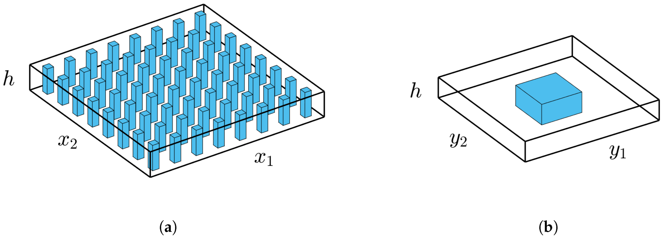
Figure 2.
Finite element procedure of SOTS for the Mindlin plate problem.
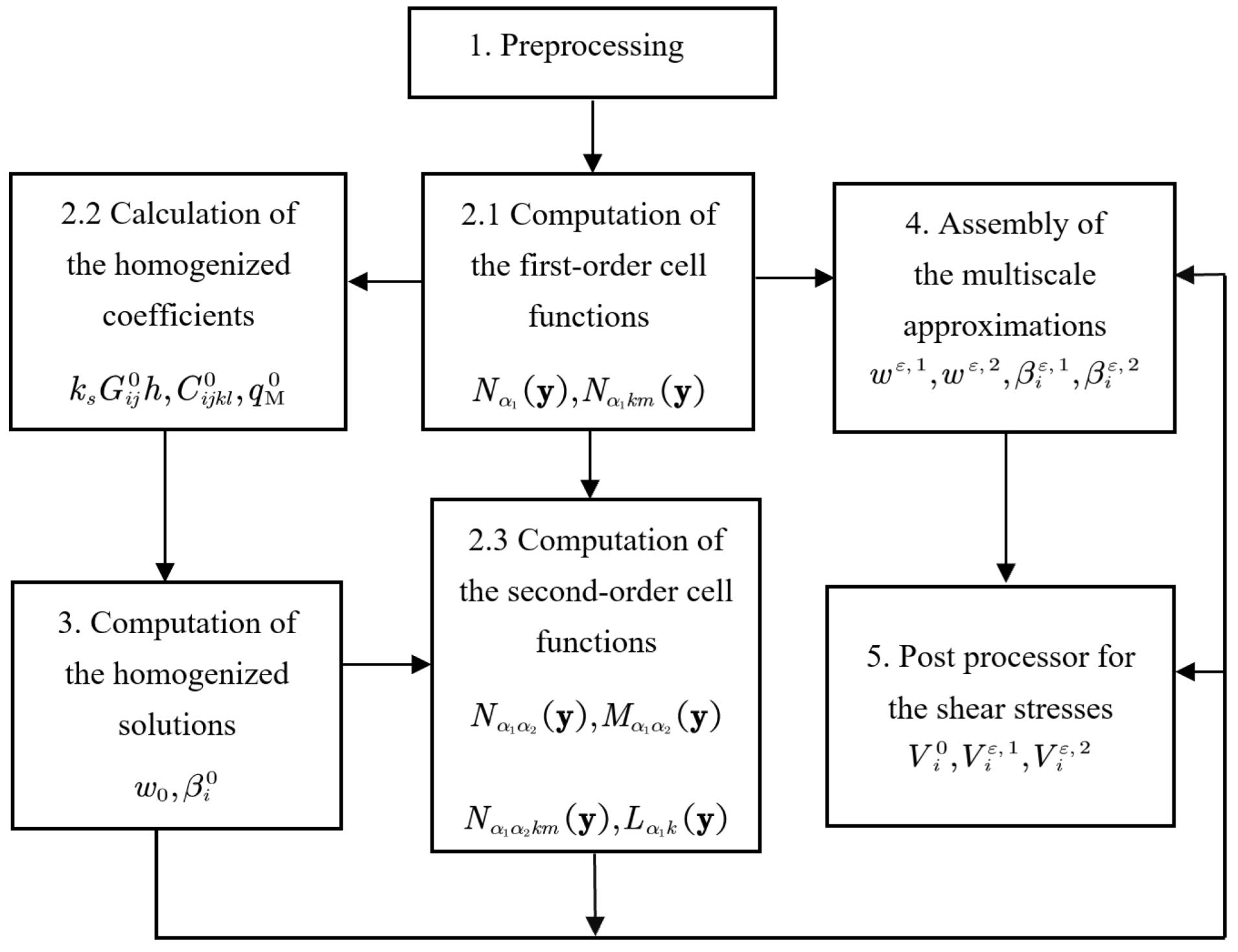
Figure 3.
Macro domain and cell domain Y with constituent materials and (). (a) Macroscopic domain ; (b) Microscopic cell domain Y.
Figure 3.
Macro domain and cell domain Y with constituent materials and (). (a) Macroscopic domain ; (b) Microscopic cell domain Y.
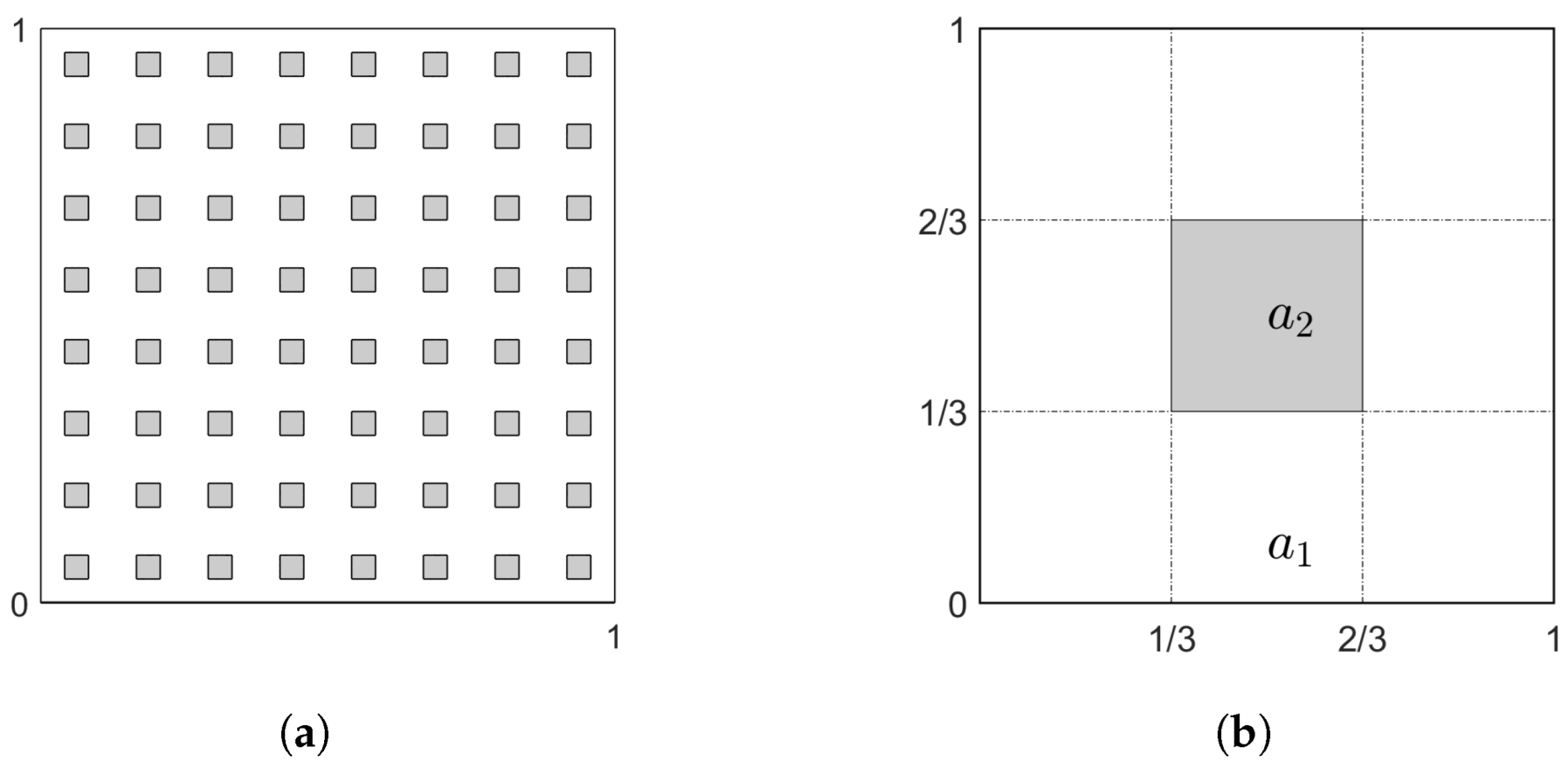
Figure 4.
Convergence of the deflection and the rotations with decreasing .
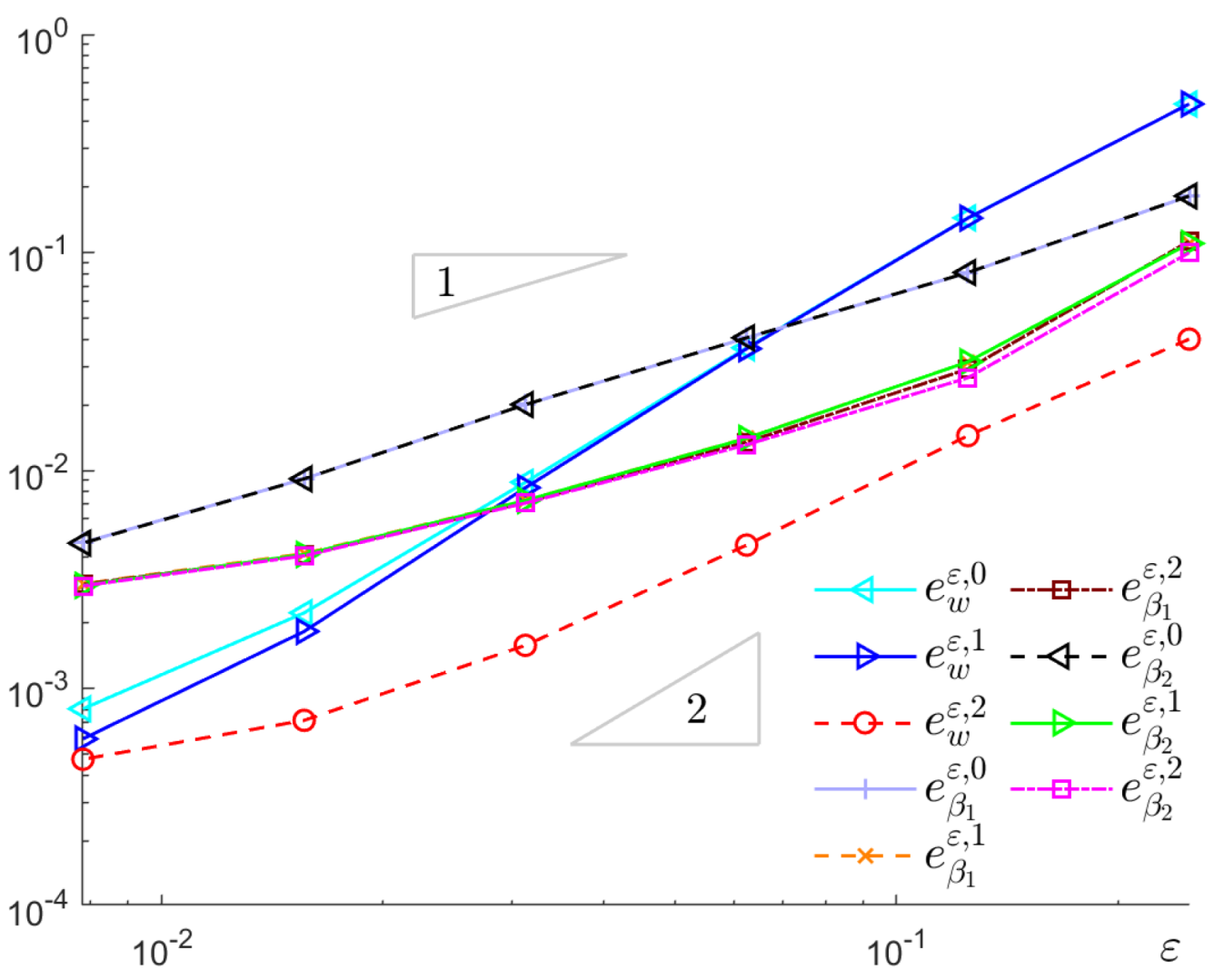
Figure 5.
Approximation of the deflection by the SOTS computation (). (a) ; (b) ; (c) ; (d).
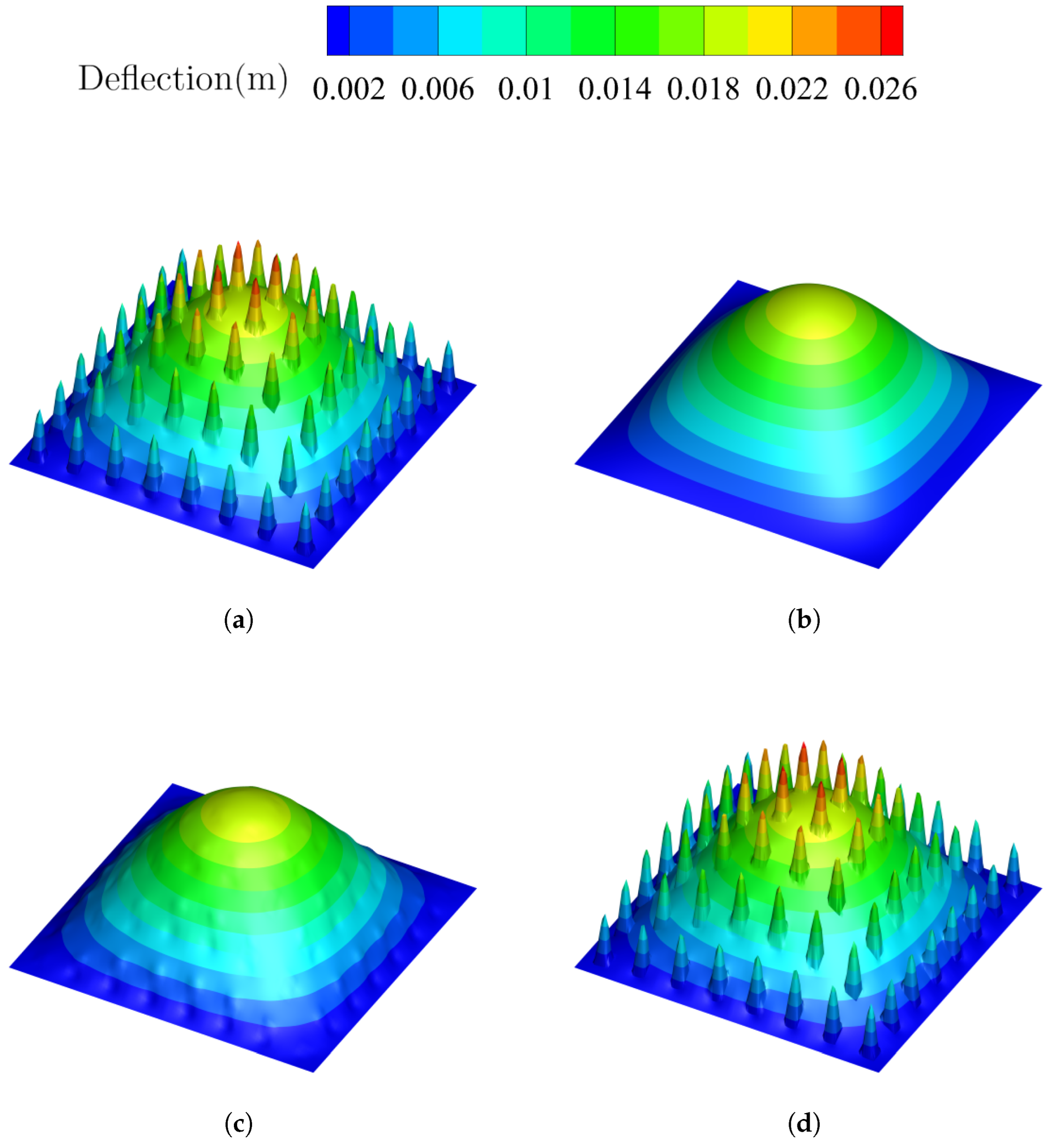
Figure 6.
Approximation of the rotations and by the SOTS computation (). (a) ; (b) ; (c) ; (d) .
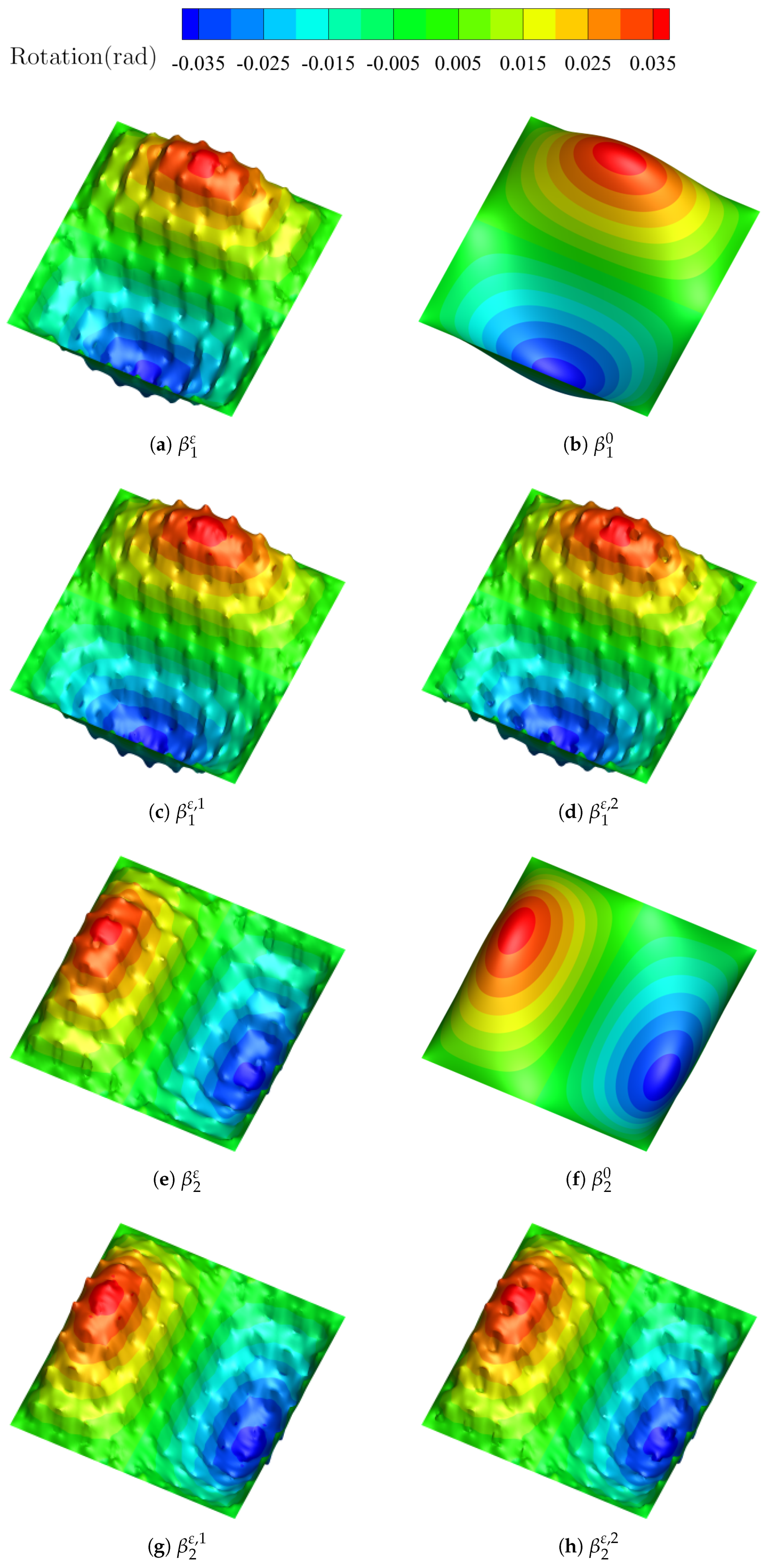
Figure 7.
Approximation of the shear stresses and by the SOTS computation ().
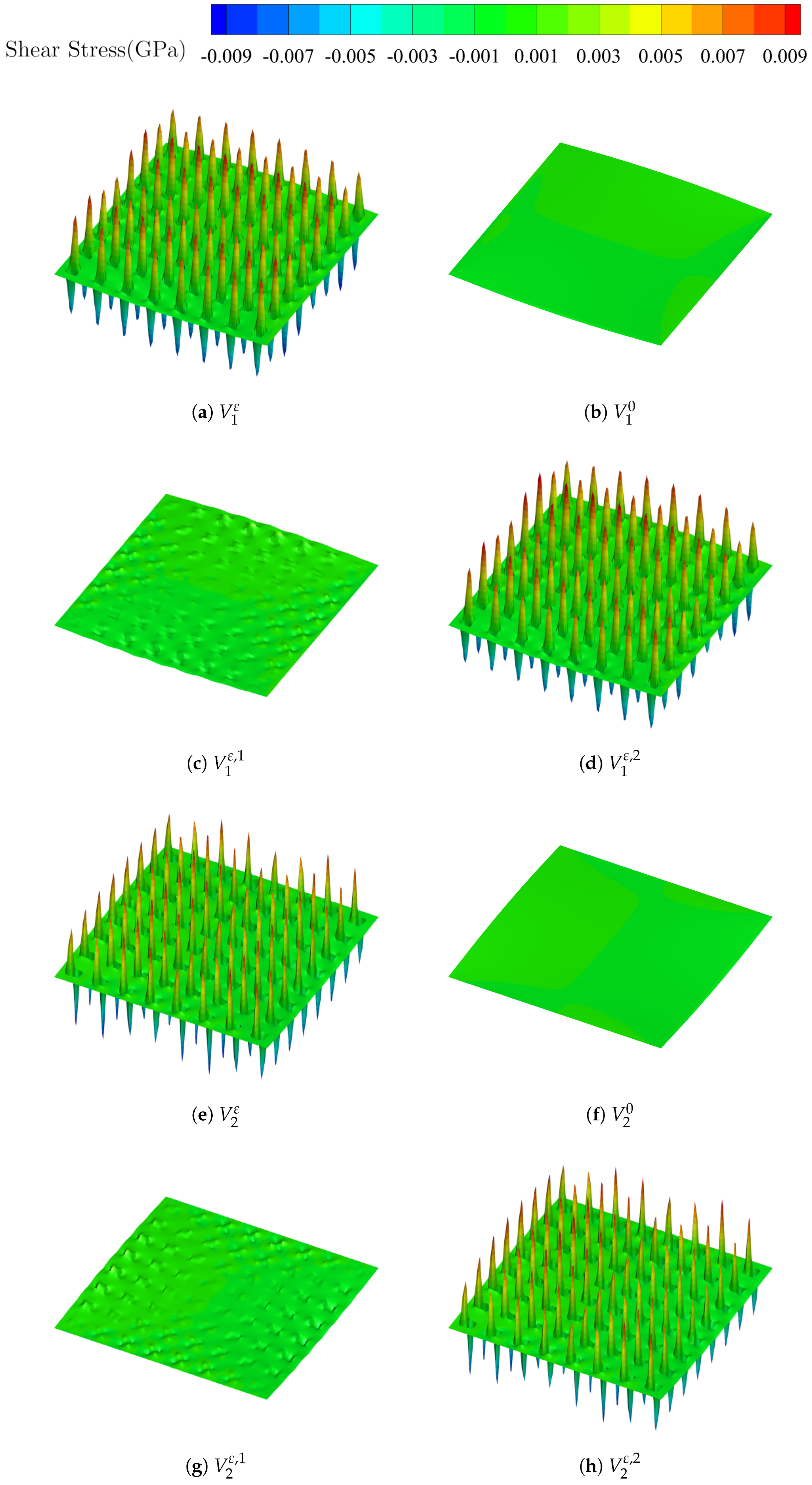
Figure 8.
Approximation of the shear stresses and along the diagonal line ().
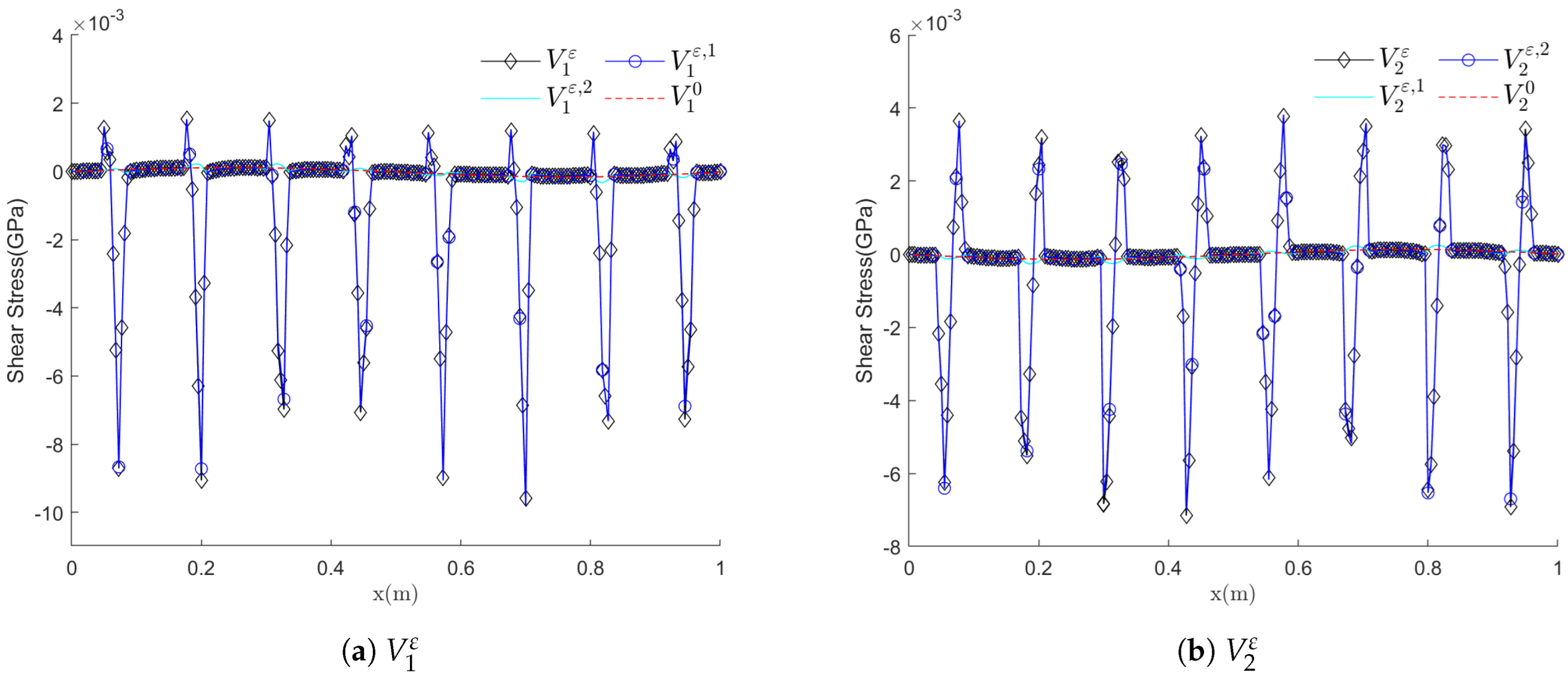
Figure 9.
Approximation of the deflection by the SOTS computation (, ).
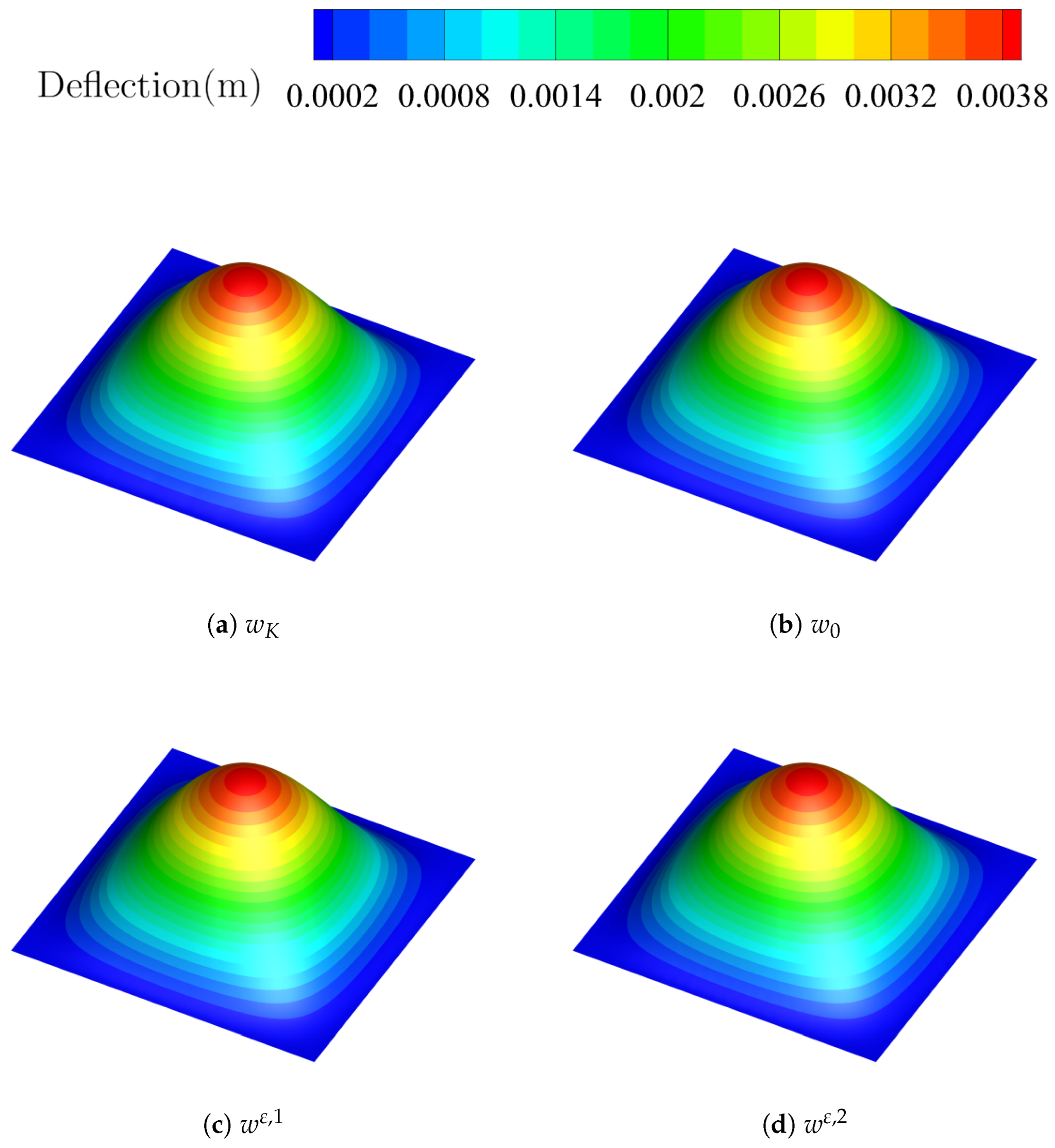
Figure 10.
Approximation of the rotations and by the SOTS computation (, ).
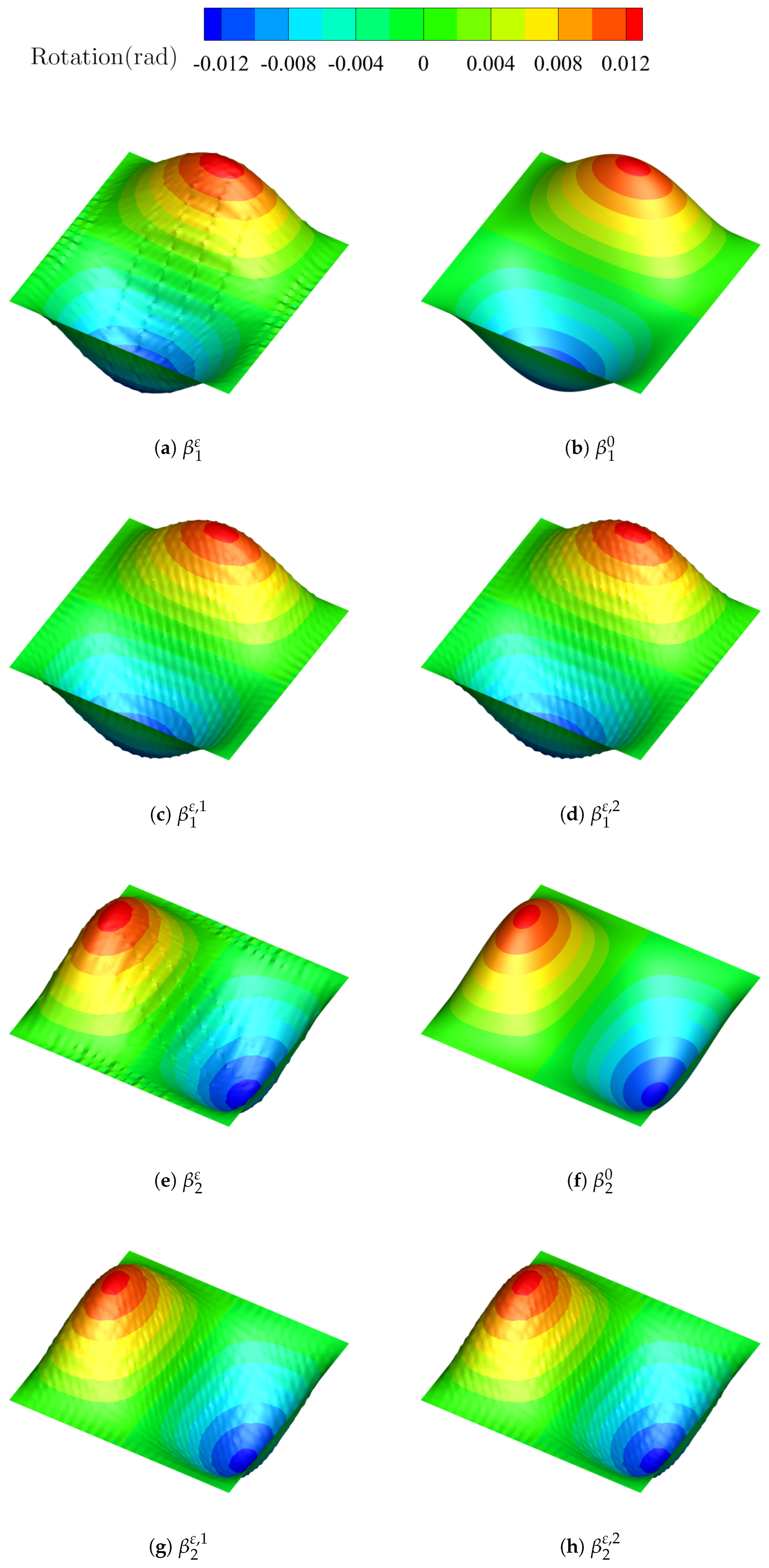
Figure 11.
Macro region and single cell region Y of the beam problem ().
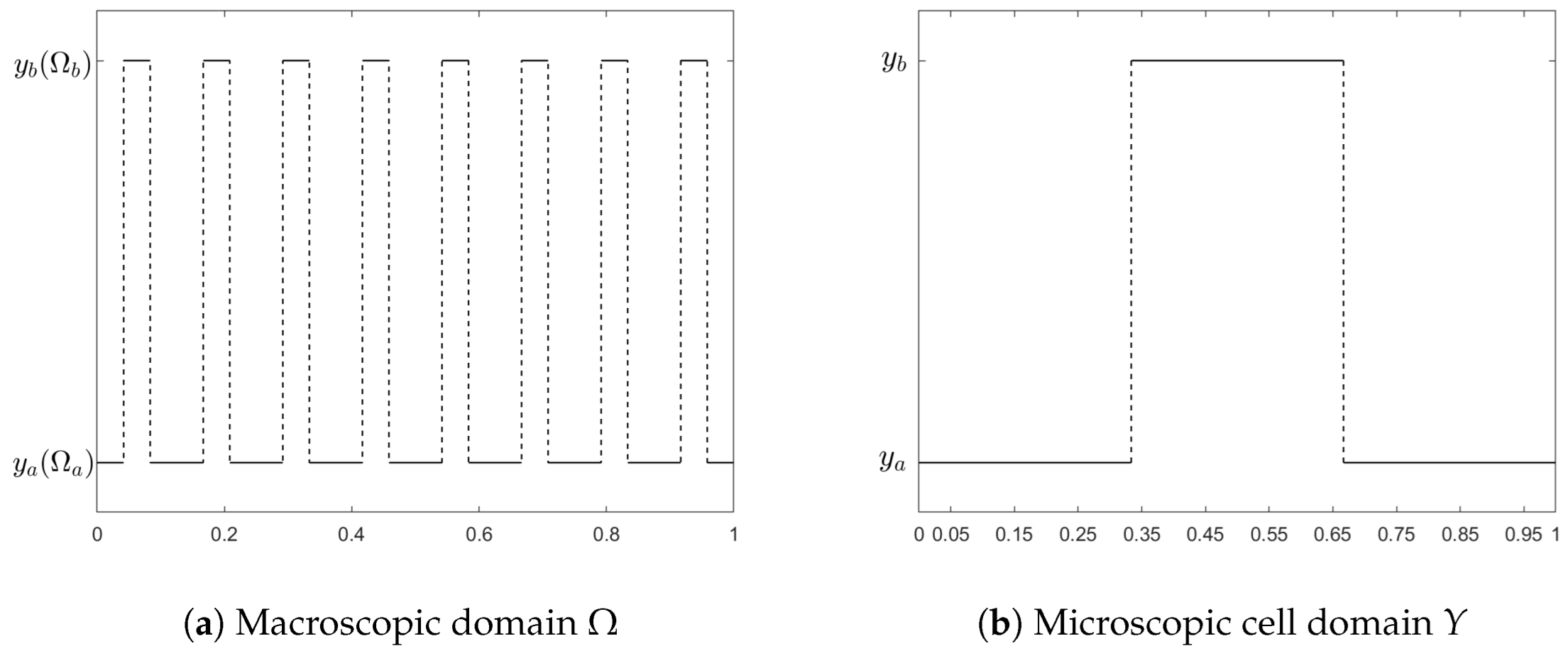
Figure 12.
Comparison of computed deflections and rotations with , and .
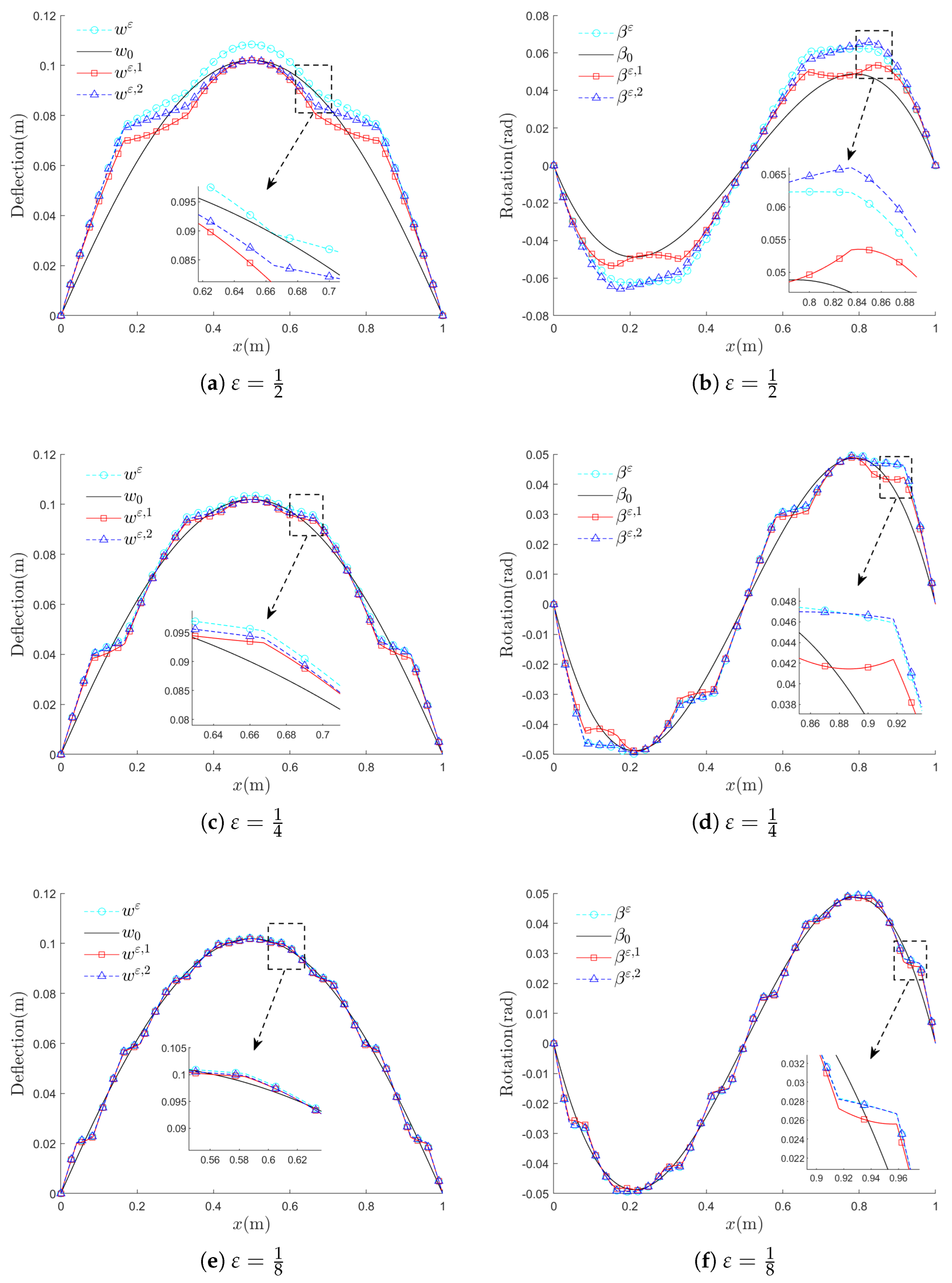
Figure 13.
Convergence of the deflection and the rotation with decreasing .
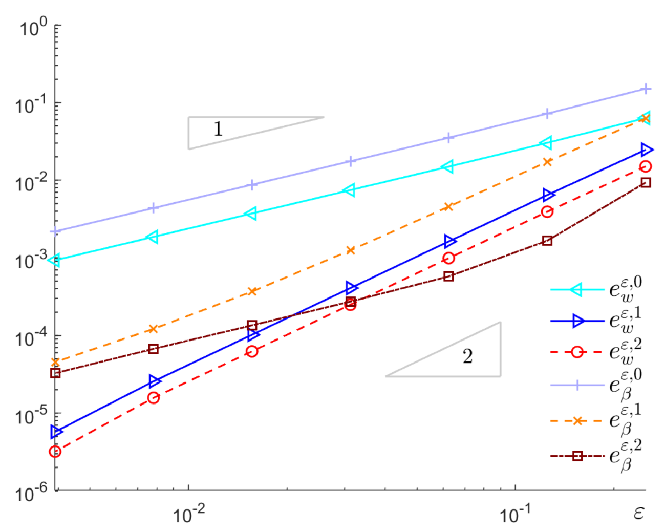
Figure 14.
Approximation of the deflection and the rotation by the SOTS computation ().
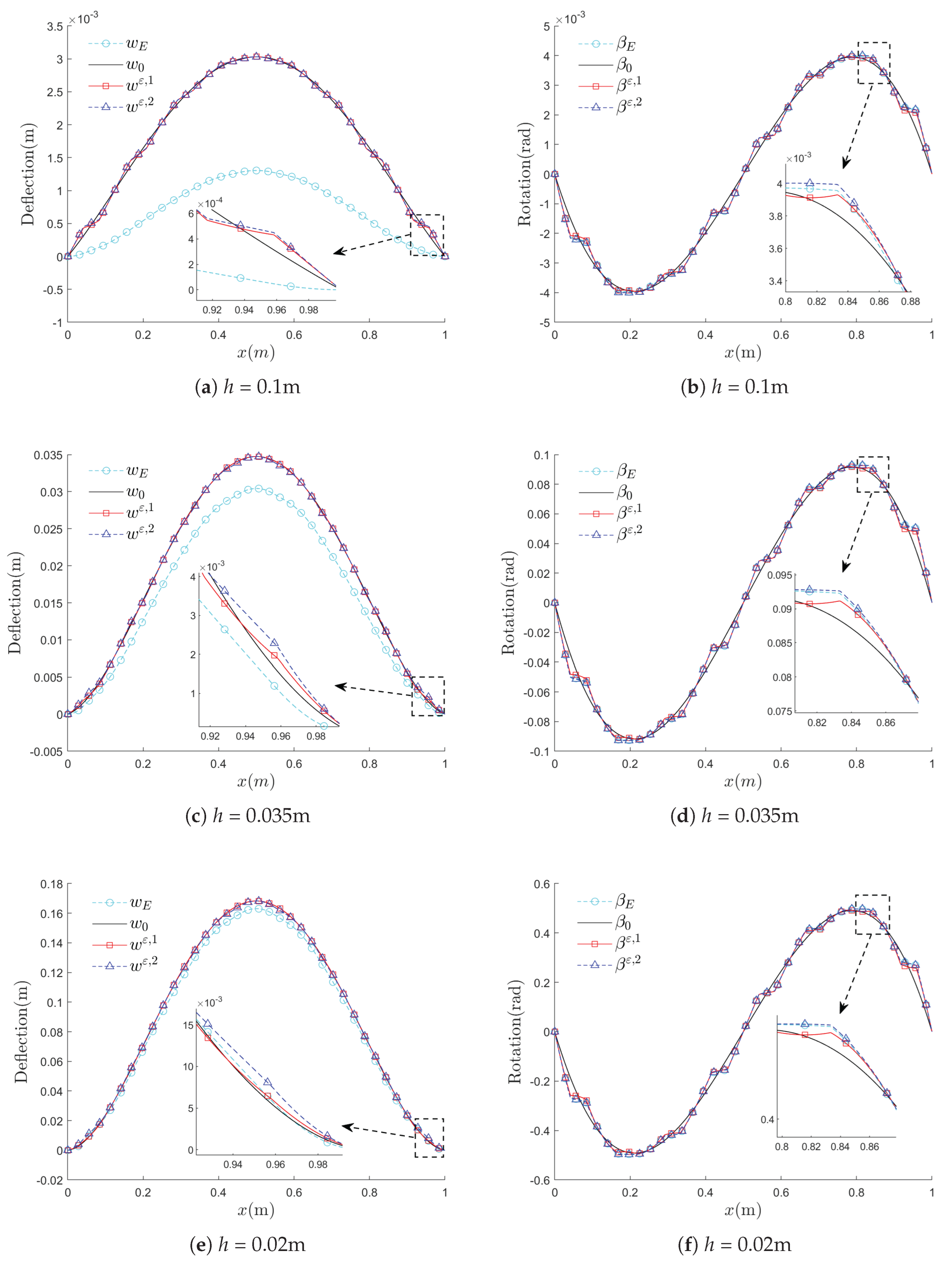

Table 1.
Mesh information and CPU time for general FE and SOTS asymptotic computation.
| Classical FE computation | Two-scale computation | |||||||
|---|---|---|---|---|---|---|---|---|
| FE Nodes | 2921 | 11537 | 45857 | 182849 | 730241 | 2918657 | 197 | 12321 |
| FE Elements | 5696 | 22784 | 91136 | 364544 | 1458176 | 5832704 | 356 | 24200 |
| CPU Time(s) | 0.988 | 3.539 | 18.313 | 74.263 | 622.632 | 5501.666 | 0.093 | 8.578 |
Table 2.
Computed relative -errors for the Mindlin plate with different .
| 4.8002E-1 | 4.8032E-1 | 4.0015E-2 | 1.8134E-1 | 1.0996E-1 | 1.1268E-1 | 1.8159E-1 | 1.0997E-1 | 9.9784E-2 | |
| 1.4407E-1 | 1.4375E-1 | 1.4428E-2 | 8.0707E-2 | 3.1478E-2 | 2.9195E-2 | 8.0852E-2 | 3.1478E-2 | 2.6609E-2 | |
| 3.6506E-2 | 3.6172E-2 | 4.5398E-3 | 4.0564E-2 | 1.4067E-2 | 1.3478E-2 | 4.0605E-2 | 1.4028E-2 | 1.3113E-2 | |
| 8.8193E-3 | 8.3226E-3 | 1.5738E-3 | 2.0023E-2 | 7.2921E-3 | 7.1350E-3 | 2.0044E-2 | 7.2757E-3 | 7.0789E-3 | |
| 2.2198E-3 | 1.8241E-3 | 7.1274E-4 | 9.1498E-3 | 4.1504E-3 | 4.0925E-3 | 9.1432E-3 | 4.1134E-3 | 4.0514E-3 | |
| 8.0502E-4 | 5.8576E-4 | 4.7236E-4 | 4.6591E-3 | 3.0136E-3 | 2.9979E-3 | 4.6346E-3 | 2.9669E-3 | 2.9514E-3 |
Table 3.
Composite Mindlin plate approaching the composite Kirchhoff plate ().
| 1.1271 | 1.1270 | 1.1363 | 2.4425E-1 | 2.4039E-1 | 2.3275E-1 | 2.4422E-1 | 2.4035E-1 | 2.3274E-1 | |
| 7.7704E-1 | 7.7707E-1 | 7.7860E-1 | 1.4543E-1 | 1.3928E-1 | 1.3810E-1 | 1.4543E-1 | 1.3932E-1 | 1.3812E-1 | |
| 8.4653E-1 | 8.4654E-1 | 8.4700E-1 | 1.4078E-1 | 1.3938E-1 | 1.3937E-1 | 1.4078E-1 | 1.3938E-1 | 1.3937E-1 | |
| 8.4770E-1 | 8.4771E-1 | 8.4791E-1 | 1.3969E-1 | 1.3929E-1 | 1.3928E-1 | 1.3969E-1 | 1.3929E-1 | 1.3928E-1 |
Table 4.
Composite Mindlin plate approaching the composite Kirchhoff plate ().
| 3.7340E-1 | 3.7337E-1 | 3.7931E-1 | 1.5980E-1 | 1.5433E-1 | 1.4895E-1 | 1.5980E-1 | 1.5433E-1 | 1.4954E-1 | |
| 1.5855E-1 | 1.5855E-1 | 1.5938E-1 | 9.4118E-2 | 8.4455E-2 | 7.2935E-2 | 9.4118E-2 | 8.4501E-2 | 7.2891E-2 | |
| 2.0104E-1 | 2.0104E-1 | 2.0134E-1 | 6.5862E-2 | 6.2822E-2 | 6.1235E-2 | 6.5862E-2 | 6.2846E-2 | 6.1228E-2 | |
| 2.0388E-1 | 2.0388E-1 | 2.0403E-1 | 6.1348E-2 | 6.0448E-2 | 5.9565E-2 | 6.1348E-2 | 6.0442E-2 | 5.9572E-2 |
Table 5.
Composite Mindlin plate approaching the composite Kirchhoff plate ().
| 1.1742E-1 | 1.1742E-1 | 1.2157E-1 | 1.0402E-1 | 8.6248E-2 | 8.4552E-2 | 1.0402E-1 | 8.6256E-2 | 8.3637E-2 | |
| 4.0151E-2 | 4.0147E-2 | 3.8461E-2 | 8.4931E-2 | 7.3972E-2 | 5.9328E-2 | 8.4931E-2 | 7.3956E-2 | 5.9577E-2 | |
| 1.0786E-2 | 1.0789E-2 | 1.0505E-2 | 3.7998E-2 | 3.2589E-2 | 2.8209E-2 | 3.7998E-2 | 3.2581E-2 | 2.8388E-2 | |
| 8.4341E-3 | 8.4346E-3 | 8.3463E-3 | 3.0168E-2 | 2.8329E-2 | 2.5397E-2 | 3.0168E-2 | 2.8321E-2 | 2.5489E-2 |
Table 6.
Computed relative -errors for the Timoshenko beam with different .
| 6.3204E-2 | 2.4709E-2 | 1.5073E-2 | 1.5090E-1 | 6.2674E-2 | 9.3377E-3 | |
| 3.0314E-2 | 6.4404E-3 | 3.9261E-3 | 7.2027E-2 | 1.7268E-2 | 1.6630E-3 | |
| 1.4972E-2 | 1.6276E-3 | 9.9237E-4 | 3.5300E-2 | 4.5739E-3 | 5.7680E-4 | |
| 7.4627E-3 | 4.0824E-4 | 2.4907E-4 | 1.7546E-2 | 1.2491E-3 | 2.7353E-4 | |
| 3.7286E-3 | 1.0223E-4 | 6.2463E-5 | 8.7584E-3 | 3.6755E-4 | 1.3517E-4 | |
| 1.8640E-3 | 2.5668E-5 | 1.5758E-5 | 4.3770E-3 | 1.2178E-4 | 6.7338E-5 | |
| 9.3197E-4 | 5.7469E-6 | 3.2017E-6 | 2.1881E-3 | 4.5484E-5 | 3.2711E-5 |
Table 7.
Approximation of the homogenized Euler beam ( = 0.02).
| 9.5292E-2 | 1.4726E-1 | |
| 2.7921E-2 | 7.0550E-2 | |
| 4.6500E-3 | 3.5153E-2 | |
| 2.7279E-3 | 2.3052E-2 |
Table 8.
Composite Timoshenko beam approaching the composite Euler beam ().
| 1.3653 | 1.3700 | 1.3779 | 1.4292E-1 | 5.0342E-2 | 1.6830E-2 | |
| 1.5184 | 1.5193 | 1.5211 | 6.9814E-2 | 1.2038E-2 | 8.7056E-3 | |
| 1.5552 | 1.5555 | 1.5559 | 3.4706E-2 | 5.1497E-3 | 3.9123E-3 | |
| 1.5449 | 1.5450 | 1.5452 | 2.2997E-2 | 3.9031E-3 | 2.5664E-3 |
Table 9.
Composite Timoshenko beam approaching the composite Euler beam ().
| 8.8101E-2 | 8.9562E-2 | 8.2858E-2 | 1.4672E-1 | 5.8046E-2 | 9.5688E-3 | |
| 1.6484E-1 | 1.6498E-1 | 1.6314E-1 | 7.0325E-2 | 1.4389E-2 | 3.4649E-3 | |
| 1.8606E-1 | 1.8609E-1 | 1.8563E-1 | 3.4635E-2 | 3.1767E-3 | 2.5024E-3 | |
| 1.8617E-1 | 1.8618E-1 | 1.8599E-1 | 2.2993E-2 | 2.7956E-3 | 1.4163E-3 |
Table 10.
Composite Timoshenko beam approaching the composite Euler beam ().
| 3.9508E-2 | 4.0083E-2 | 4.2898E-2 | 1.4710E-1 | 5.8696E-2 | 9.3389E-3 | |
| 3.8995E-2 | 3.9078E-2 | 3.6491E-2 | 7.0391E-2 | 1.4654E-2 | 3.1435E-3 | |
| 5.7812E-2 | 5.7823E-2 | 5.7254E-2 | 3.4641E-2 | 3.2293E-3 | 2.3076E-3 | |
| 5.8164E-2 | 5.8169E-2 | 5.7925E-2 | 2.2992E-2 | 2.7895E-3 | 1.4008E-3 |
Disclaimer/Publisher’s Note: The statements, opinions and data contained in all publications are solely those of the individual author(s) and contributor(s) and not of MDPI and/or the editor(s). MDPI and/or the editor(s) disclaim responsibility for any injury to people or property resulting from any ideas, methods, instructions or products referred to in the content. |
© 2025 by the authors. Licensee MDPI, Basel, Switzerland. This article is an open access article distributed under the terms and conditions of the Creative Commons Attribution (CC BY) license (http://creativecommons.org/licenses/by/4.0/).
Copyright: This open access article is published under a Creative Commons CC BY 4.0 license, which permit the free download, distribution, and reuse, provided that the author and preprint are cited in any reuse.


