
Submitted:
12 December 2024
Posted:
12 December 2024
You are already at the latest version
Abstract
This study presents a refined beam theory aimed at overcoming the limitations of classical approaches, such as the Euler-Bernoulli and Timoshenko models, which often neglect transverse shear deformation and rotational inertia effects. These limitations become significant when analyzing thick beams or structures made of advanced materials. The proposed theory assumes a linearly elastic, homogeneous, and isotropic material with a uniform rectangular cross-section. While maintaining simplicity and a strong resemblance to the classical Bernoulli-Euler theory, this refined approach provides a more accurate framework for analyzing beam bending. A simplified governing equation is derived, offering a straightforward formulation suitable for practical engineering applications. General analytical solutions are obtained for thick isotropic beams under various boundary conditions, including simply supported, cantilever, and fixed configurations, subjected to both uniformly and unevenly distributed loads. The study derives expressions for transverse displacement, strain components, stress components, and internal forces. The accuracy and applicability of the proposed theory are validated by comparing its results with those of other advanced shear deformation theories, demonstrating its effectiveness for precise structural analysis.
Keywords:
refined beam theory
; structural analysis
; transverse displacement
; axial stress
; transverse shear stress
; thick beams
; analytical solutions
1. Introduction
The analysis of beam bending is a fundamental aspect of structural mechanics and engineering design, forming the basis for understanding how beams behave under various loading conditions. Classical theories, such as the Euler-Bernoulli and Timoshenko models, have long provided robust frameworks for analyzing bending mechanics [1, 2]. These theories, however, are built on simplifying assumptions, such as the neglect of transverse shear deformation and rotational inertia effects. While effective for slender beams, these limitations reduce their applicability to thick beams or materials with complex mechanical properties, underscoring the need for more advanced models.
To address these challenges, researchers have developed higher-order shear deformation theories (HSDTs). These models go beyond the assumptions of classical theories, incorporating additional terms to capture the effects of transverse shear deformation more accurately. Significant advancements in this area include the parabolic shear deformation theories proposed by Levinson [3], Shames et al. [4], Rehfield and Murty [5], Krishna Murty [6], Baluch, Azad, and Khidir [7], as well as Bhimaraddi and Chandrashekhara [8]. These theories introduce a refined variation of axial displacement along the thickness coordinate, inherently satisfying shear stress-free boundary conditions at the top and bottom surfaces of the beam. Consequently, they eliminate the need for shear correction factors, offering a more precise approach to modeling beam deformation.
The importance of transverse shear deformation becomes evident when analyzing thick or short beams. Compared to slender beams, shear deformation effects can significantly increase deflections, decrease buckling loads, and reduce vibrational frequencies. To quantify these effects, nondimensionalization of these quantities is essential, as highlighted by Shimpi et al. [9]. Furthermore, studies such as [10-12] underscore the critical role of transverse shear in accurately predicting deformation behavior.
In the quest to overcome the limitations of first-order shear deformation theories, researchers have developed numerous HSDTs [13-22]. These theories provide more accurate estimations of beam deformation but often introduce additional governing equations and unknown functions, increasing computational demands. Wang et al. [23] noted that the complexity of these models can be a barrier to their practical application, emphasizing the importance of balancing accuracy and computational efficiency.
Beyond polynomial-based models, refined theories employing trigonometric and hyperbolic functions have gained attention. Vlasov and Leont’ev [24] and Stein [25] introduced sinusoidal kinematic descriptions for thick beams. However, these theories fall short in satisfying shear stress-free boundary conditions at the beam surfaces. Building on this, Ghugal and Sharma [26, 27] proposed a hyperbolic shear deformation theory for static and dynamic analysis, while Ghugal and Dahake [28] and others [29, 30] applied trigonometric models to analyze flexural behavior under various loading and support conditions. These advancements represent important strides in addressing the limitations of earlier models.
A noteworthy contribution to the field is the work of Canales and Mantari [31], who developed an analytical approach for static bending of thick isotropic rectangular beams with diverse boundary conditions. By combining boundary discontinuous Fourier series with shear deformation theories, they derived stress and displacement solutions. However, their work leaves some aspects, such as bending and shear stress distributions at built-in ends, unexplored, suggesting room for further refinement.
Comprehensive reviews by Ghugal and Shimpi [32] and Sayyad and Ghugal [33] highlight the dominance of Navier-type closed-form solutions for simply supported beams in the literature. Analytical solutions for beams with built-in ends or specialized loading conditions remain limited, emphasizing the need for continued innovation in this domain.
Alternative methodologies have also emerged, such as splitting transverse displacement into sub-components. Studies [34, 35] introduced a system of two governing equations, inertially coupled in dynamic cases and decoupled for static problems. Similar approaches appear in [36-39], offering a fresh perspective on addressing shear deformation.
Despite these advancements, challenges persist. Bathe [40] pointed out the issue of artificial stiffening in lower-order, displacement-based finite elements when analyzing thin beams. This phenomenon, known as shear locking, leads to underestimated displacements. Significant research has been conducted to develop finite elements resistant to shear locking, as documented in [41, 42].
Recent studies [43-50] reflect the ongoing evolution of shear deformation theories, highlighting their relevance in modern structural analysis. These advancements ensure that the field remains active, with researchers continually striving to refine models and expand their applicability to complex engineering problems.
In future research, this simplified theory can be expanded to broader applications. It provides a solid foundation for analyzing the behavior of beams on an elastic foundation [51-53]. Its application can help address complex structural challenges, such as accounting for foundation stiffness and interaction effects, while maintaining computational efficiency. Additionally, it can be adapted to study more advanced cases, including non-uniform foundations or dynamic loading conditions.
The purpose of this work is to develop a refined theory that addresses the shortcomings of the classical theory and presents fundamental relationships in a simple and practical form for implementation. The derivations are focused on plane elements with rectangular cross-sections. However, by adjusting the geometric characteristics, the theory can be applied to elements with arbitrary cross-sections. Analytical solutions for the static bending of beams with built-in boundary conditions are derived. To demonstrate the effectiveness of the proposed theory, illustrative examples of the static bending of shear-deformable isotropic rectangular beams are provided. The numerical results are compared with other refined theories to validate the accuracy and reliability of the proposed approach.
2. Assumptions Underlying the Proposed Theory
The assumptions underlying the theoretical formulation of the proposed model are as follows:
1) The beam under investigation, illustrated in Figure 1, is located in the 0 – x1 – x2 – x3 Cartesian coordinate system and spans the region:
This is example 1 of an equation:
here, x1, x2 and x3 represent the Cartesian coordinates, while l and b denote the beam's length and width in the x1- and x2-directions, respectively. The thickness of the beam along the x3-axis is represented by h.
2) The beam consists of a homogeneous, linearly elastic, isotropic material and the applied loads are static and uniformly or non-uniformly distributed along the beam.
3) The beam's boundary conditions are defined at the ends x1=0 and x1=l, where variationally consistent conditions are applied.
4) The deformation and stress distribution along the x3-axis follow predefined laws, ensuring consistency with the refined beam theory framework.
5) The transverse shear deformation varies according to a prescribed function, capturing its dependence on the thickness coordinate.
6) The horizontal displacement component does not experience any tensile or compressive deformation, maintaining the integrity of the beam's axial behavior.
3. Current Theory: Displacement Functions, Strains, Stresses, Cross-Sectional Bending Moment, and Shearing Force
3.1. Development of Theory
The stress-strain state in the exact formulation is defined by the following relationships of elasticity theory:
- Equilibrium equations expressed in terms of stress components:
where are the normal stresses directed along the coordinate axes, is shear stress perpendicular to these axes, are the components of the body force acting along the coordinate planes.
- Kinematic relations (Cauchy):
where are the linear strains, is the shear strain, and are the displacement components along the coordinate axes .
- Physical relations (Hooke's law):
where E is the modulus of elasticity of the material, and is Poisson's ratio.
This theory is based on the integral characteristics of stresses and displacements:
where are the bending moment and axial force due to normal stress , is the axial force, are the normal displacement and the angle of cross-sectional rotation, are the horizontal displacements along the and axes, respectively.
By integrating equation (1) and considering (4) in the absence of body forces, we obtain the equilibrium equations in terms of internal forces:
Thus, from Hooke's law (3) and the notations (4), the following expressions are derived:
where are the bending and shear stiffness.
Substituting (6) into the first equation of system (5), we obtain:
Equation (7) can be rewritten in operator form:
where L is a linear operator.
We can express the solution of equation (8) as follows:
From here, we obtain the components of the displacements:
From the second equation of (5), considering (6) and (9), we derive the governing equation for determining the function W(x1):
The unused Hooke's law equation (3) is integrated:
As a result, taking into account (4), we obtain:
Another integral of the same law can be written as:
where are the vertical displacements along the and axes, respectively
From these expressions (11) and (12), the displacements and are determined.
Within the framework of the classical Euler-Bernoulli beam theory, the stresses can be represented as follows:
where is the transverse shear stress distribution function, is the normal transverse stress distribution function.
Assuming the stress in the form of (13), we obtain:
3.2. The Displacement Field
A Based on the aforementioned assumptions and results, the displacement field of the present beam theory is defined as follows:
where W(x1) is the deflection function, is the shear modulus of the beam material, is the intensity of external load.
3.3. Expressions for Strains
The normal and shear strains, derived within the framework of linear elasticity theory from the displacement field described by equations (13) and (14), are expressed as follows:
3.4. Expressions for stresses
Normal bending and transverse shear stresses are determined using one-dimensional constitutive laws (13) and (15), and they are expressed as follows:
3.5. Expression for the cross-sectional bending moment and shear force
The cross-sectional bending moment and shear force for a beam are defined as follows:
where M, Q are the bending moment and shear force.
3.6. Governing Differential Equations and Boundary Conditions
Using equations (5) and (9), we obtain the basic equation:
The corresponding consistent natural boundary conditions are obtained in the following form:
1) If the ends of the beam are hinge-supported, the boundary conditions are as follows:
2) If the ends of the beam are fixed, the boundary conditions are as follows:
3) If the ends of the beam are free, the boundary conditions are as follows:
Thus, this refined theory makes it possible to determine the stress-strain state of the beam, resolves the contradictions of the classical beam bending theory, and thereby enables calculations in a precise formulation.
The calculation of any beam using the proposed refined theory is carried out according to the following algorithm:
1) The deflection function is determined by solving equation (18) while satisfying one of the boundary conditions specified in (19)–(21).
2) The displacement components are calculated using formula (14).
3) The strain components are determined based on formula (15).
4) The stress components are found using formula (16).
5) The internal forces in the beam are computed according to formula (17).
4. Numerical Results
This section presents numerical results related to the static bending of shear-deformable isotropic prismatic rectangular beams, provided both in tabular form and as graphical representations.
Example 1. A simply supported beam (SS beam) subjected to a uniformly distributed transverse load.
In this example, the beam ends at and are simply supported. The boundary conditions for W corresponding to the SS beam are as follows:
1. Boundary conditions at beam end :
2. Boundary conditions at beam end :
Example 2. Clamped-clamped beam (CC beam) subjected to a uniformly distributed transverse load.
In this example, the beam ends at and are clamped. The boundary conditions for W corresponding to the CC beam are as follows:
1. Boundary conditions at beam end :
2. Boundary conditions at beam end :
Example 3: A cantilever beam (FC beam) subjected to a uniformly distributed transverse load.
In this example, the beam end at is free, while the beam end at is clamped. The boundary conditions for W corresponding to the FC beam are as follows:
1. Boundary conditions at beam end :
2. Boundary conditions at beam end :
Example 4: Simply supported beam subjected to a varying load.
The simply supported beam originates at the left support and is supported at and , with a varying load applied along its length.
The boundary conditions for W are defined by formulas (22) and (23).
The non-dimensional transverse displacement W, non-dimensional axial stress , and non-dimensional transverse shear stress for the beam are defined as follows:
Numerical results for , and from Examples 1 to 4, calculated using the proposed theory for various beam thickness-to-length ratios (h/l), are presented in Tables 1 to 10. These results are compared with corresponding values obtained from the two-dimensional theory of elasticity, single-variable beam theory, two-variable theory, Levinson beam theory, Timoshenko beam theory, and Bernoulli-Euler beam theory to demonstrate the effectiveness of the proposed approach.
While deriving the results shown in Tables 1 to 10, the following points have been taken into account:
1) The Poisson’s ratio μ is assumed to be 0.3.
2) For Examples 1–3, the beam thickness-to-length ratio (h/l) is considered as 0.01, 0.05, 0.10, and 0.15. In Example 4, the beam length-to-thickness ratio (S=l/h) is taken as 4 and 10.
3) The numerical results for based on the Levinson beam theory and single-variable beam theory, and for and based on the single-variable beam theory, are as reported by Shimpi et al. [9].
4) The numerical results for , , and , obtained using the two-dimensional theory of elasticity (plane stress), two-variable theory, Timoshenko beam theory, and Bernoulli-Euler beam theory, are computed by the authors [48].
a) Expressions from the respective references cited in the tables are used for these calculations.
b) For the Timoshenko beam theory, a shear correction factor of 5/6 is applied.
) for Example 1 (simply supported beam, Figure 1) computed using the proposed theory, with a comparison to existing results for .
5. Discussion of Numerical Results for Static Beam Bending
This section provides an analysis of the numerical results related to the static bending (Examples 1 to 4, presented in Tables 1 to 10 and in Figure 2, Figure 3, Figure 4, Figure 5, Figure 6 and Figure 7) of isotropic prismatic rectangular beams with shear deformability.
Table 1, Table 2, Table 3, Table 4, Table 5, Table 6, Table 7, Table 8, Table 9 and Table 10 present numerical results for the dimensionless transverse deflection , the dimensionless axial stress , and the dimensionless shear stress of the beam, corresponding to SS (simply supported), CC (clamped-clamped), and FC (fixed-free) beams. Based on these numerical results, the following observations can be made:
1. Observations on the numerical results for the SS beam (Example 1) presented in Table 1, Table 2 and Table 3.
For the simply supported (SS) beam analyzed using the present theory, the maximum percentage difference in predicting is -0.37% (for h/l=0.15), in predicting is 0.00% (for h/l=0.15), and in predicting is 0.00% (for h/l=0.15). For other beam thickness-to-length ratios (h/l=0.01, h/l=0.05, and h/l=0.10), the percentage differences are very small.
2. Observations on the numerical results for the CC beam (Example 2) presented in Table 4, Table 5 and Table 6.
For the clamped-clamped (CC) beam analyzed using the present theory, the maximum percentage difference in predicting is -1.70% (for h/l=0.15), in predicting is 1.25% (for h/l=0.15), and in predicting is 0.00% (for h/l=0.15). For other beam thickness-to-length ratios (h/l=0.01, h/l=0.05, and h/l=0.10), the percentage differences remain relatively small, indicating a high level of accuracy for the present theory across various scenarios.
3. Observations on the numerical results for the FC beam (Example 3) presented in Table 7, Table 8 and Table 9.
For the fixed-free (FC) beam analyzed using the present theory, the maximum percentage difference in predicting is -0.82% (for h/l=0.15), in predicting is 0.06% (for h/l=0.15), and in predicting is 0.00% (for h/l=0.15). For other beam thickness-to-length ratios (h/l=0.01, h/l=0.05, and h/l=0.10), the percentage differences are minimal, indicating the robustness and accuracy of the present theory in capturing the behavior of shear-deformable beams under this boundary condition.
4. Observations on the numerical results for the SS beam subjected to a non-uniformly distributed load (Example 4) are presented in Table 10 and in Figure 2, Figure 3, Figure 4, Figure 5, Figure 6 and Figure 7.
For a simply supported (SS) beam subjected to a non-uniformly distributed load and analyzed using the present theory, the maximum percentage differences in , , and for l/h=4 and l/h=10 are negligible. These results demonstrate the accuracy and reliability of the proposed approach in predicting the response of beams under varying load conditions.
For SS (simply supported), CC (clamped-clamped), and FC (fixed-free) beams, the results obtained using the present theory demonstrate excellent agreement with the exact solutions derived from the two-dimensional theory of elasticity for both thin and shear-deformable beams. Furthermore, the predictions of the present theory align remarkably well with the corresponding results of the Levinson beam theory, the single-variable beam theory, and the two-variable theory for thin and shear-deformable beams.
The classical Bernoulli-Euler beam theory neglects the effects of transverse shear deformation, resulting in underestimated predictions for shear-deformable beams. While the displacements computed by the Bernoulli-Euler theory may coincide with exact elasticity solutions in some cases, this agreement fails to account for transverse shear deformation. Consequently, the Bernoulli-Euler theory is incapable of accurately determining transverse shear stresses through the constitutive relationship between shear stress and shear strain.
In contrast, the present theory incorporates transverse shear deformation effects, enabling the direct calculation of transverse shear stresses through the constitutive relationship. This makes the proposed theory more accurate and suitable for analyzing shear-deformable beams.
The Timoshenko beam theory, being a first-order shear deformation theory, assumes a uniform distribution of transverse shear stress across the beam thickness. As a result, the transverse shear stresses derived from this theory remain constant through the thickness and do not satisfy the stress-free boundary conditions on the beam surfaces at z=±h/2. The present theory, however, accurately predicts transverse shear stresses that satisfy these boundary conditions, varying quadratically through the beam thickness and being zero at z=±h/2.
Additionally, the accuracy of the Timoshenko beam theory is influenced by the use of a shear correction factor, which introduces dependency and potential inaccuracies in the results. The present theory eliminates this issue by not requiring a shear correction factor for its computations, further enhancing its reliability and precision in shear-deformable beam analysis.
6. Conclusions
The refined beam bending theory proposed in this study provides a significant step forward in addressing the challenges associated with classical approaches. By incorporating the effects of transverse shear deformation and eliminating the reliance on shear correction factors, this theory ensures higher accuracy and broader applicability, particularly for thick and shear-deformable beams. Its governing equations, formulated in a straightforward and consistent manner, enable precise solutions that satisfy boundary conditions and accommodate diverse loading scenarios.
Furthermore, comparative analyses with existing refined theories and two-dimensional elasticity solutions validate the theory’s effectiveness, while numerical examples demonstrate its applicability to various beam configurations, including simply supported, clamped, and cantilever beams under both uniform and non-uniform loads. This combination of simplicity, accuracy, and practicality highlights the potential of the proposed theory to enhance structural modeling and engineering design processes.
Looking ahead, the flexibility and robustness of this approach create opportunities for future research. Extending the theory to beams with complex geometries, anisotropic materials, and dynamic loading conditions could significantly expand its utility, further bridging the gap between theoretical development and real-world engineering applications.
Author Contributions
Conceptualization, S.A.; methodology, S.A. and A.N.; software, A.N.; validation, D.M. and T.A.; formal analysis, D.M. and T.A.; investigation, S.A. and A.N.; resources, A.N.; data curation, D.M. and T.A.; writing—original draft preparation, S.A. and A.N.; writing—review and editing, S.A. and A.N.; visualization, A.N.; supervision, A.N.; project administration, A.N. All authors have read and agreed to the published version of the manuscript.
Funding
This research was funded by the Science Committee of the Ministry of Science and Higher Education of the Republic of Kazakhstan (AP22684709— An improved method for calculating bending and free vibration of functionally graded beams resting on an elastic foundation).
Data Availability Statement
Available on request.
Conflicts of Interest
The authors declare no conflict of interest.
References
- Carrera, E.; Giunta, G.; Petrolo, M. Beam Structures: Classical and Advanced Theories, A John Wiley & Sons Ltd Publication, New Delhi, 2011; pp. 1-42.
- Timoshenko, S.P.; Goodier, J.N. Theory of Elasticity, Third Int. Ed.; McGraw-Hill, Singapore, 1970.
- Levinson, M. A new rectangular beam theory. J. of Sound and Vibration 1981, 74, 81–87. [Google Scholar] [CrossRef]
- Shames, I.H.; Dym, C.L. Energy and Finite Element Methods in Structural Mechanics, Hemisphere Publishing Corporation, Washington, 1985, pp. 185-204.
- Rehfield, L.W.; Murthy, P.L.N. Toward a new engineering theory of bending: fundamentals. AIAA J. 1982, 20, 693–699. [Google Scholar] [CrossRef]
- Krishna Murty, A.V. Towards a consistent beam theory. AIAA J. 1984, 22, 811–816. [Google Scholar] [CrossRef]
- Baluch, M.H.; Azad, A.K.; Khidir, M.A. Technical theory of beams with normal strain. ASCE J. of Engineering Mechanics 1984, 110, 1233–1237. [Google Scholar] [CrossRef]
- Bhimaraddi, A.; Chandrashekhara, K. Observations on higher order beam Theory. ASCE J. of Aerospace Engineering 1993, 6, 408–413. [Google Scholar] [CrossRef]
- Shimpi, R.P.; Shetty, R.A.; Guha, A. A Simple Single Variable Shear Deformation Theory for a Rectangular Beam. Proceedings of the Institution of Mechanical Engineers, Part C: Journal of Mechanical Engineering Science 2017, 231, 4576–4591. [Google Scholar] [CrossRef]
- Simão, P.D. Influence of Shear Deformations on the Buckling of Columns using the Generalized Beam Theory and Energy Principles. European Journal of Mechanics - A/Solids 2017, 61, 216–234. [Google Scholar] [CrossRef]
- Kiendl, J.; Auricchio, F.; Hughes, T.J.R.; Reali, A. Single-variable Formulations and Isogeometric Discretizations for Shear Deformable Beams. Computer Methods in Applied Mechanics and Engineering 2015, 284, 988–1004. [Google Scholar] [CrossRef]
- Saoud, K.S.; Le Grognec, P. An Enriched 1D Finite Element for the Buckling Analysis of Sandwich Beam-columns. Computational Mechanics 2016, 57, 887–900. [Google Scholar] [CrossRef]
- Xia, Y.-M.; Li, S.-R.; Wan, Z.-Q. Bending Solutions of FGM Reddy–Bickford Beams in Terms of Those of the Homogenous Euler–Bernoulli Beams. Acta Mechanica Solida Sinica 2019, 32, 499–516. [Google Scholar] [CrossRef]
- Chen, S.; Geng, R.; Li, W. Vibration analysis of functionally graded beams using a higher-order shear deformable beam model with rational shear stress distribution. Composite Structures 2021, 277, 114586. [Google Scholar] [CrossRef]
- Khorshidi, K.; Rezaeisaray, M.; Karimi, M. Analytical approach to energy harvesting of functionally graded higher-order beams with proof mass. Acta Mechanica 2022, 233, 4273–4293. [Google Scholar] [CrossRef]
- Benatta, M.A.; Mechab, I.; Tounsi, A.; Adda Bedia, E.A. Static Analysis of Functionally Graded Short Beams Including Warping and Shear Deformation Effects. Computational Materials Science 2008, 44, 765–773. [Google Scholar] [CrossRef]
- Karama, M.; Afaq, K.S.; Mistou, S. Mechanical Behaviour of Laminated Composite Beam by the New Multilayered Laminated Composite Structures Model with Transverse Shear Stress Continuity. International Journal of Solids and Structures 2003, 40, 1525–1546. [Google Scholar] [CrossRef]
- Mahi, A.; Adda Bedia, E.A.; Tounsi, A.; Mechab, I. An Analytical Method for Temperature-dependent Free Vibration Analysis of Functionally Graded Beams with General Boundary Conditions. Composite Structures 2010, 92, 1877–1887. [Google Scholar] [CrossRef]
- Mantari, J.L.; Canales, F.G. A Unified Quasi-3D HSDT for the Bending Analysis of Laminated Beams. Aerospace Science and Technology 2016, 54, 267–275. [Google Scholar] [CrossRef]
- Shi, G.; Voyiadjis, G.Z. A Sixth-order Theory of Shear Deformable Beams with Variational Consistent Boundary Conditions. ASME Journal of Applied Mechanics 2011, 78, 021019. [Google Scholar] [CrossRef]
- Benatta, M.A.; Tounsi, A.; Mechab, I.; Bachir Bouiadjra, M. Mathematical Solution for Bending of Short Hybrid Composite Beams with Variable Fibers Spacing. Applied Mathematics and Computation 2009, 212, 337–348. [Google Scholar] [CrossRef]
- Karttunen, A.T.; Von Hertzen, R. Variational Formulation of the Static Levinson Beam Theory. Mechanics Research Communications 2015, 66, 15–19. [Google Scholar] [CrossRef]
- Wang, C.M.; Reddy, J.N.; Lee, K.H. Shear Deformable Beams and Plates, Relationships with Classical Solutions, Elsevier Science Ltd, New York, 2000; pp. 1-7.
- Vlasov, V.Z.; Leont’ev, U.N. Beams, plates and shells on elastic foundations, Iseral Program for Scientific Translation Ltd., Jerusalem, 1966; pp. 1-8.
- Stein, M. Vibration of beams and plate strips with three-dimensional flexibility. ASME Jl. of Appl. Mech. 1989, 56, 228–231. [Google Scholar] [CrossRef]
- Ghugal, Y.M.; Sharma, R. A hyperbolic shear deformation theory for flexure and vibration of thick isotropic beams. Intl. Jl. of Comput. Meth. 2009, 6, 585–604. [Google Scholar] [CrossRef]
- Ghugal, Y.M; Sharma, R. A refined shear deformation theory for flexure of thick beams. Latin Ame. Jl. of Solids and Structs. 2011, 8, 183–193. [Google Scholar] [CrossRef]
- Ghugal, Y.M; Dahake, A.G. Flexure of simply supported thick beams using refined shear deformation theory. Intl. Jl. of Civ., Envir., Struct., Construct. and Architect. Engg. 2013, 7, 99–108. [Google Scholar]
- Dahake, A.G; Ghugal, Y.M. A trigonometric shear deformation theory for flexure of thick beam. Procedia Engg., Elsevier 2013, 51, 1–7. [Google Scholar] [CrossRef]
- Jadhav, V.A.; Dahake, A.G. Bending analysis of deep beam using refined shear deformation theory. Intl. Jl. of Engg. Res. 2016, 5, 526–531. [Google Scholar] [CrossRef]
- Canales, F.G.; Mantari, J.L. Boundary discontinuous Fourier analysis of thick beams with clamped and simply supported edges via CUF. Chinese Journal of Aeronautics 2017, 30, 1708–1718. [Google Scholar] [CrossRef]
- Ghugal, Y.M.; Shmipi, R.P. A review of refined shear deformation theories for isotropic and anisotropic laminated beams. Jl. of Reinfor. Plast. and Compos. 2001, 20, 255–272. [Google Scholar] [CrossRef]
- Sayyad, A.S.; Ghugal, Y.M. Bending, buckling and free vibration of laminated composite and sandwich beams: A critical review of literature. Jl. of Compos. Structs. 2017, 171, 486–504. [Google Scholar] [CrossRef]
- Shimpi, R.P. Refined Plate Theory and Its Variants. AIAA Journal 2002, 40, 137–146. [Google Scholar] [CrossRef]
- Shimpi, R.P.; Patel, H.G.; Arya, H. New First-order Shear Deformation Plate Theories. ASME Journal of Applied Mechanics 2007, 74, 523–533. [Google Scholar] [CrossRef]
- El Meiche, N.; Tounsi, A.; Ziane, N.; Mechab, I.; Adda Bedia, E.A. A New Hyperbolic Shear Deformation Theory for Buckling and Vibration of Functionally Graded Sandwich Plate. International Journal of Mechanical Sciences 2011, 53, 237–247. [Google Scholar] [CrossRef]
- Daouadji, T.H.; Henni, A.H.; Tounsi, A.; Adda Bedia, E.A. A New Hyperbolic Shear Deformation Theory for Bending Analysis of Functionally Graded Plates. Modelling and Simulation in Engineering 2012, 6, 29. [Google Scholar] [CrossRef]
- Daouadji, T.H.; Tounsi, A.; Adda Bedia, E.A. A New Higher Order Shear Deformation Model for Static Behavior of Functionally Graded Plates. Advances in Applied Mathematics and Mechanics 2013, 5, 351–364. [Google Scholar] [CrossRef]
- Shimpi, R.P.; Guruprasad, P.J.; Pakhare, K.S. Single Variable New First-order Shear Deformation Theory for Isotropic Plates. Latin American Journal of Solids and Structures 2018, 15, 1–25. [Google Scholar] [CrossRef]
- Bathe, K.J. Finite Element Procedures, Prentice Hall, New Jersey, 1996; pp. 116-120.
- Reddy, J.N. On Locking-free Shear Deformable Beam Finite Elements. Computer Methods in Applied Mechanics and Engineering 1997, 149, 113–132. [Google Scholar] [CrossRef]
- Ainsworth, M.; Pinchedez, K. The hp-MITC Finite Element Method for the Reissner–Mindlin Plate Problem. Journal of Computational and Applied Mathematics 2002, 148, 429–462. [Google Scholar] [CrossRef]
- Canales, F.G.; Mantari, J.L. Buckling and Free Vibration of Laminated Beams with Arbitrary BoundaryConditions using a Refined HSDT. Composites Part B: Engineering 2016, 100, 136–145. [Google Scholar] [CrossRef]
- Sayyad, A.S.; Ghugal, Y.M.; Naik, N.S. Bending Analysis of Laminated Composite and Sandwich Beams According to Refined Trigonometric Beam Theory. Curved and Layered Structures 2015, 2, 279–289. [Google Scholar] [CrossRef]
- Sayyad, A.S.; Ghugal, Y.M.; Shinde, P.N. Stress Analysis of Laminated Composite and Soft Core Sandwich Beams using a Simple Higher Order Shear Deformation Theory. Journal of Serbian Society for Computational Mechanics 2015, 9, 15–35. [Google Scholar] [CrossRef]
- Boutahar, Y.; Lebaal, N.; Bassir, D. A Refined Theory for Bending Vibratory Analysis of Thick Functionally Graded Beams. Mathematics 2021, 9, 1422. [Google Scholar] [CrossRef]
- Ghugal, Y.M.; Dahake, A.G. Flexure of narrow rectangular deep beams with built-in ends. Journal of Structural Engineering, 2019, 45, 497–511. [Google Scholar]
- Shimpi, R.P.; Guruprasad, P.J.; Pakhare, K.S. Simple Two Variable Refined Theory for Shear Deformable Isotropic Rectangular Beams. J. Appl. Comput. Mech., 2020, 6, 394–415. [Google Scholar] [CrossRef]
- Ge, R.; Liu, F.; Wang, C.; Ma, L.; Wang, J. Calculation of Critical Load of Axially Functionally Graded and Variable Cross-Section Timoshenko Beams by Using Interpolating Matrix Method. Mathematics 2022, 10, 2350. [Google Scholar] [CrossRef]
- Singh, K.; Kaur, I.; Craciun, E.-M. Study of Transversely Isotropic Visco-Beam with Memory-Dependent Derivative. Mathematics 2023, 11, 4416. [Google Scholar] [CrossRef]
- Akhazhanov, S.; Omarbekova, N.; Mergenbekova, A.; Zhunussova, G.; Abdykeshova, D. Analytical solution of beams on elastic foundation. International Journal of Geomate 2020, 73, 193–200. [Google Scholar] [CrossRef]
- Akhazhanov, S.B.; Vatin, N.I.; Akhmediyev, S.; Akhazhanov, T.; Khabidolda, O.; Nurgoziyeva, A. Beam on a two-parameter elastic foundation: Simplified finite element model. Magazine of Civil Engineering 2023, 5, 1–17. [Google Scholar] [CrossRef]
- Akhazhanov, S.; Bostanov, B.; Kaliyev, A.; Akhazhanov, T.; Mergenbekova, A. Simplified method of calculating a beam on a two-parameter elastic foundation. International Journal of Geomate 2023, 25, 33–40. [Google Scholar] [CrossRef]
- Hao-jiang, D.; De-jin, H.; Hui-ming, W. Analytical Solution for Fixed-end Beam Subjected to Uniform Load. Journal of Zhejiang University-SCIENCE 2005, 6, 779–783. [Google Scholar] [CrossRef]
- Venkatraman, B.; Patel, S.A. Structural Mechanics with Introductions to Elasticity and Plasticity, McGraw-Hill Book Company, New York, 1970, pp. 158-165.
Figure 1.
Geometry of the beam and the coordinate system.
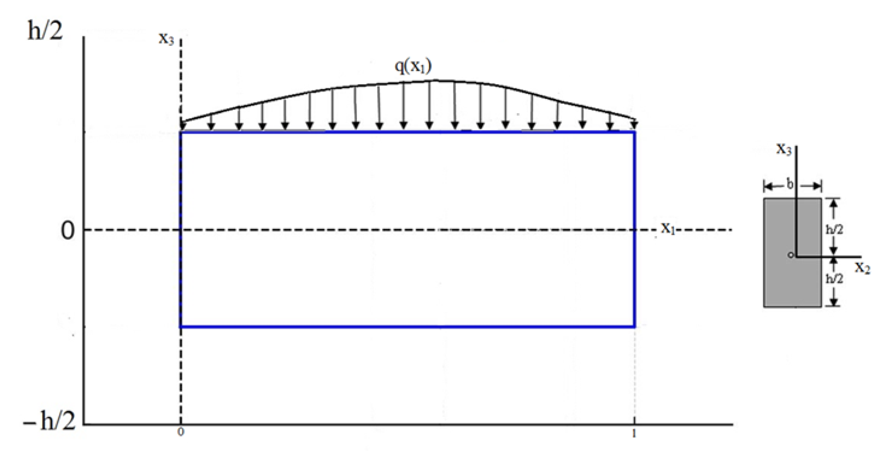
Figure 2.
Variation of transverse displacement (W) through the thickness of a simply supported beam at x=0.25l and z, subjected to a varying load, for an aspect ratio S=10 (Example 4).
Figure 2.
Variation of transverse displacement (W) through the thickness of a simply supported beam at x=0.25l and z, subjected to a varying load, for an aspect ratio S=10 (Example 4).
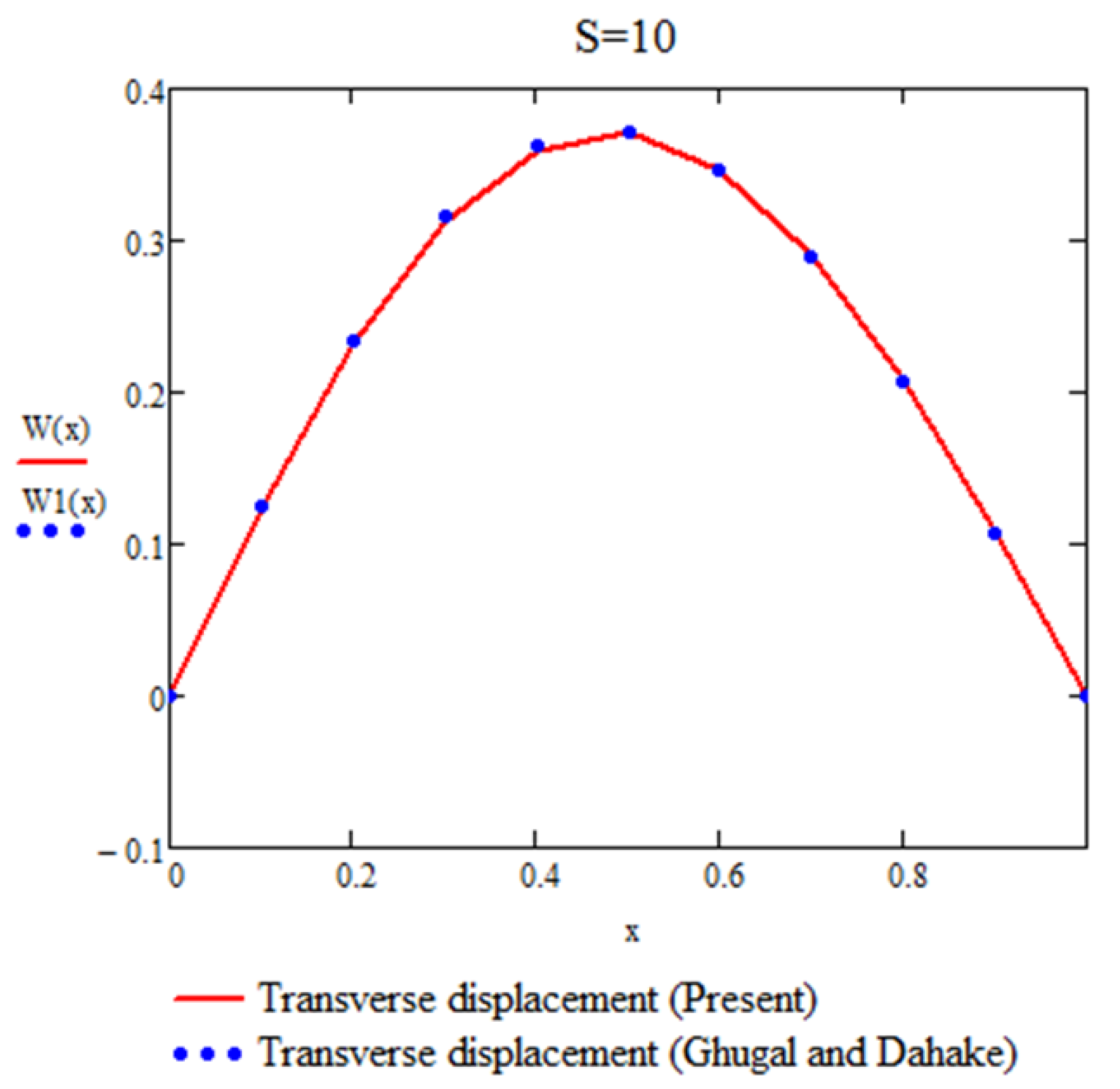
Figure 3.
Variation of axial stress (
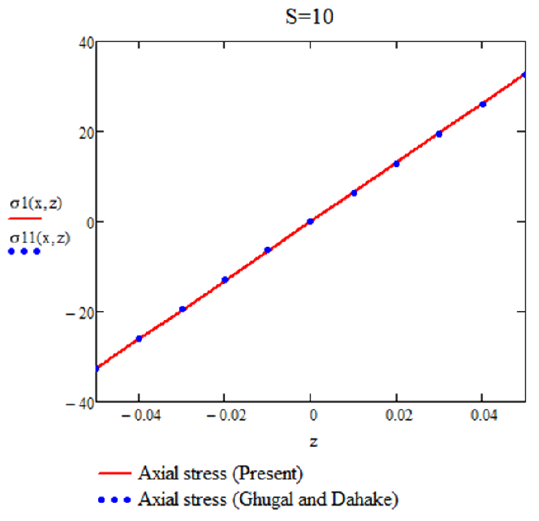
Figure 4.
Variation of shear stress (
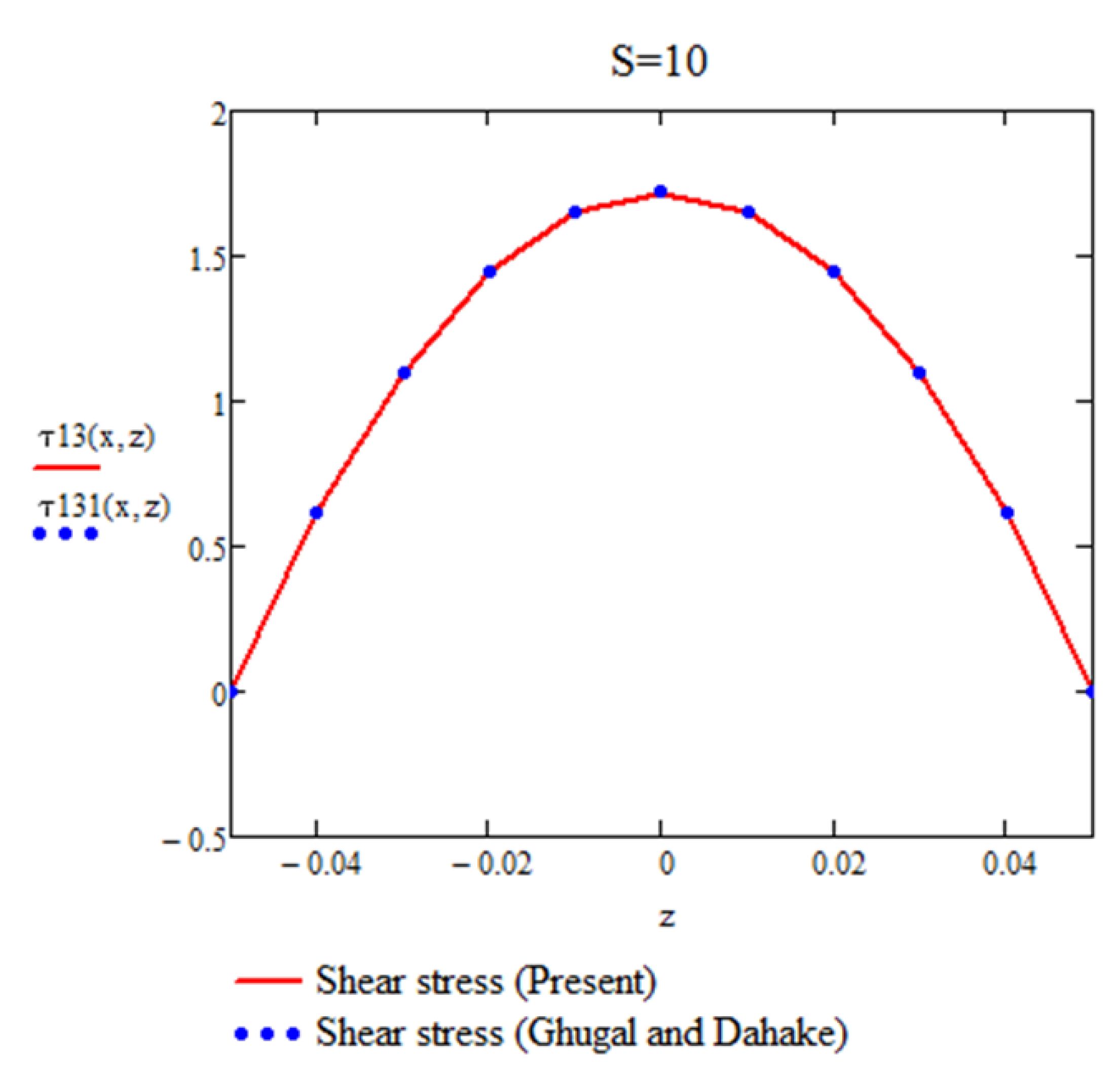
Figure 5.
Variation of transverse displacement (W) through the thickness of a simply supported beam at x=0.25l and z, subjected to a varying load, for an aspect ratio S=4 (Example 4).
Figure 5.
Variation of transverse displacement (W) through the thickness of a simply supported beam at x=0.25l and z, subjected to a varying load, for an aspect ratio S=4 (Example 4).
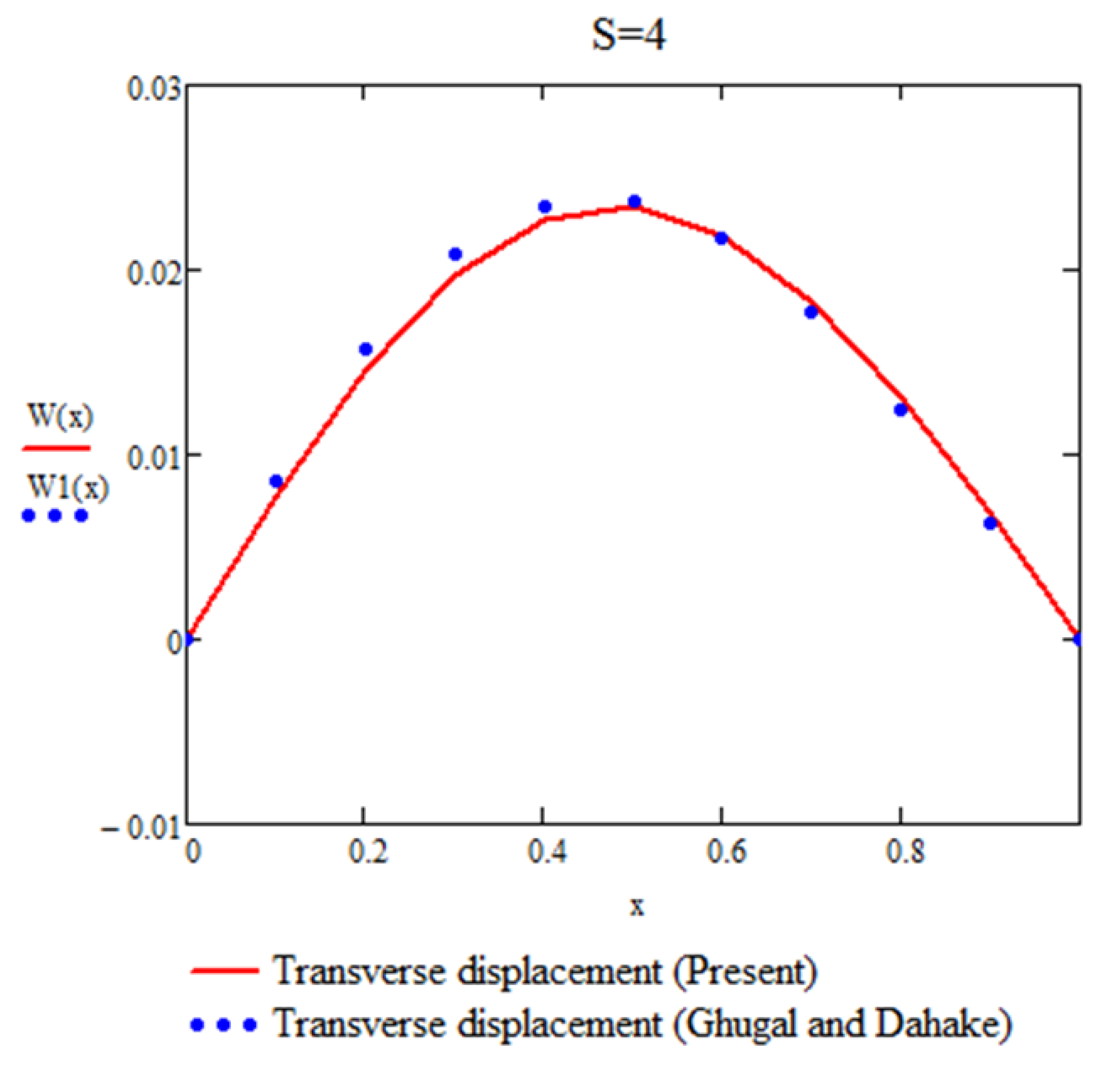
Figure 6.
Variation of axial stress (
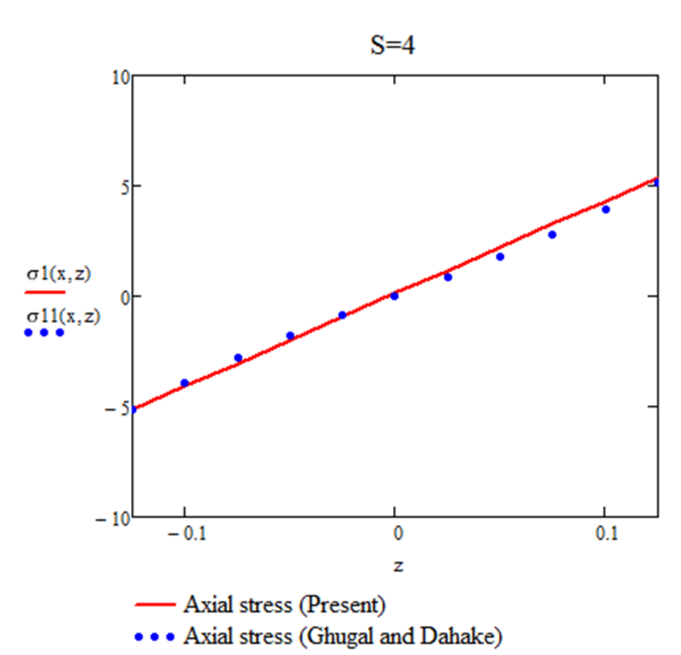
Figure 7.
Variation of shear stress (
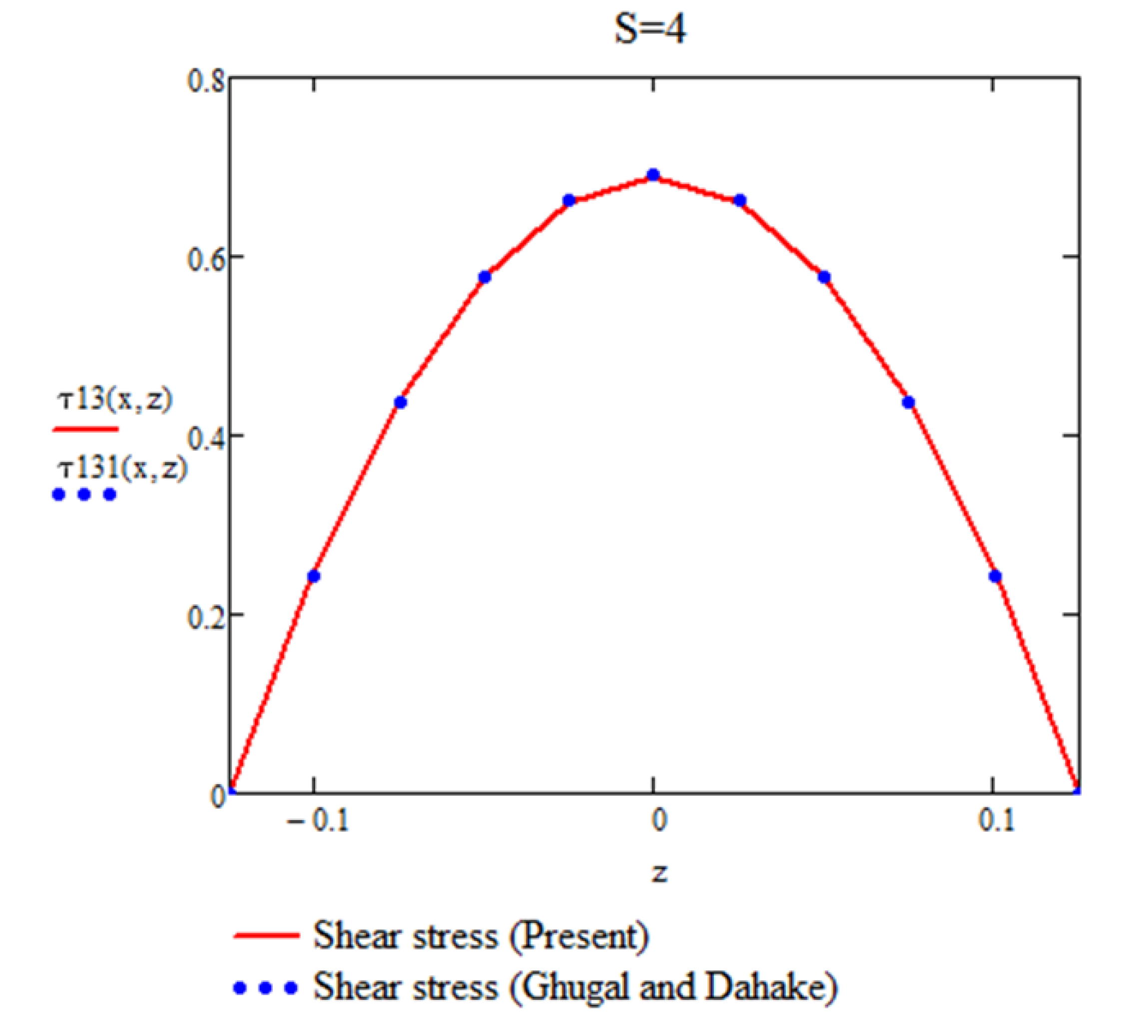

Table 1.
Non-dimensional transverse displacement (
| (Values in parentheses represent the percentage difference) | ||||
|---|---|---|---|---|
| Present | 0.01302 | 0.01308 | 0.01329 | 0.01364 |
| (0.00 %) | (-0.15 %) | (-0.22 %) | (-0.37 %) | |
| Bernoulli-Euler [4] | 0.01302 | 0.01302 | 0.01302 | 0.01302 |
| (0.00 %) | (-0.61 %) | (-2.25 %) | (-4.89 %) | |
| Timoshenko [4] | 0.01302 | 0.01310 | 0.01335 | 0.01375 |
| (0.00 %) | (0.00 %) | (0.23 %) | (0.44 %) | |
| Levinson [9] | 0.01302 | 0.01310 | 0.01335 | — |
| (0.00 %) | (0.00 %) | (0.23 %) | ||
| Single variable theory [9] | 0.01302 | 0.01310 | 0.01335 | — |
| (0.00 %) | (0.00 %) | (0.23 %) | ||
| Two variable theory [48] | 0.01302 | 0.01310 | 0.01335 | 0.01375 |
| (0.00 %) | (0.00 %) | (0.23 %) | (0.44 %) | |
| Theory of elasticity [4] | 0.01302 | 0.01310 | 0.01332 | 0.01369 |
Table 2.
Non-dimensional axial stress (
| (Values in parentheses represent the percentage difference) | ||||
|---|---|---|---|---|
| Present | 7500.12 | 300.12 | 75.12 | 33.45 |
| (0.00 %) | (0.00 %) | (0.00 %) | (0.00 %) | |
| Bernoulli-Euler [4] | 7500.00 | 300.00 | 75.00 | 33.33 |
| (0.00 %) | (-0.07 %) | (-0.27 %) | (-0.60 %) | |
| Timoshenko [4] | 7500.00 | 300.00 | 75.00 | 33.33 |
| (0.00 %) | (-0.07 %) | (-0.27 %) | (-0.60 %) | |
| Single variable theory [9] | 7500.00 | 300.26 | 75.26 | — |
| (0.00 %) | (0.02 %) | (0.08 %) | ||
| Two variable theory [48] | 7500.26 | 300.26 | 75.26 | 33.59 |
| (0.00 %) | (0.02 %) | (0.08 %) | (0.18 %) | |
| Theory of elasticity [4] | 7500.20 | 300.20 | 75.20 | 33.53 |
Table 3.
Non-dimensional shear stress (
| (Values in parentheses represent the percentage difference) | ||||
|---|---|---|---|---|
| Present | 75.00 | 15.00 | 7.50 | 5.00 |
| (0.00 %) | (0.00 %) | (0.00 %) | (0.00 %) | |
| Bernoulli-Euler [4] | 75.00 | 15.00 | 7.50 | 5.00 |
| (0.00 %) | (0.00 %) | (0.00 %) | (0.00 %) | |
| Timoshenko [4] | 50.00 | 10.00 | 5.00 | 3.33 |
| (-33.33 %) | (-33.33 %) | (-33.33 %) | (-33.33 %) | |
| Single variable theory [9] | 75.00 | 15.00 | 7.50 | — |
| (0.00 %) | (0.00 %) | (0.00 %) | ||
| Two variable theory [48] | 74.92 | 14.92 | 7.42 | 4.92 |
| (-0.11 %) | (-0.53 %) | (-1.07 %) | (-1.60 %) | |
| Theory of elasticity [4] | 75.00 | 15.00 | 7.50 | 5.00 |
Table 4.
Non-dimensional transverse displacement (
| (Values in parentheses represent the percentage difference) | ||||
|---|---|---|---|---|
| Present | 0.00260 | 0.00270 | 0.00296 | 0.00346 |
| (0.00 %) | (-0.37 %) | (-1.66 %) | (-1.70 %) | |
| Bernoulli-Euler [2, 4] | 0.00260 | 0.00260 | 0.00260 | 0.00260 |
| (-0.38 %) | (-4.06 %) | (-13.62 %) | (-26.14 %) | |
| Timoshenko [3, 4] | 0.00261 | 0.00269 | 0.00293 | 0.00334 |
| (0.00 %) | (-0.74 %) | (-2.66 %) | (-5.11 %) | |
| Levinson [9] | 0.00261 | 0.00271 | 0.00301 | — |
| (0.00 %) | (0.00 %) | (0.00 %) | ||
| Single variable theory [9] | 0.00261 | 0.00271 | 0.00301 | — |
| (0.00 %) | (0.00 %) | (0.00 %) | ||
| Two variable theory [48] | 0.00261 | 0.00269 | 0.00293 | 0.00334 |
| (0.00 %) | (-0.74 %) | (-2.66 %) | (-5.11 %) | |
| Theory of elasticity [54] | 0.00261 | 0.00271 | 0.00301 | 0.00352 |
Table 5.
Non-dimensional axial stress (
| (Values in parentheses represent the percentage difference) | ||||
|---|---|---|---|---|
| Present | -4999.70 | -199.70 | -49.70 | -21.92 |
| (0.00 %) | (0.14 %) | (0.55 %) | (1.25 %) | |
| Bernoulli-Euler [2, 4] | -5000.00 | -200.00 | -50.00 | -22.22 |
| (0.01 %) | (0.29 %) | (1.15 %) | (2.63 %) | |
| Timoshenko [3, 4] | -5000.00 | -200.00 | -50.00 | -22.22 |
| (0.01 %) | (0.29 %) | (1.15 %) | (2.63 %) | |
| Single variable theory [9] | -4999.35 | -199.35 | -49.35 | — |
| (0.01 %) | (-0.04 %) | (-0.16 %) | ||
| Two variable theory [48] | -5000.00 | -200.00 | -50.00 | -22.22 |
| (0.01 %) | (0.29 %) | (1.15 %) | (2.63 %) | |
| Theory of elasticity [54] | -4999.43 | -199.43 | -49.43 | -21.65 |
Table 6.
Non-dimensional shear stress (
| (Values in parentheses represent the percentage difference) | ||||
|---|---|---|---|---|
| Present | 75.00 | 15.00 | 7.50 | 5.00 |
| (0.00 %) | (0.00 %) | (0.00 %) | (0.00 %) | |
| Bernoulli-Euler [2, 4] | 75.00 | 15.00 | 7.50 | 5.00 |
| (0.00 %) | (0.00 %) | (0.00 %) | (0.00 %) | |
| Timoshenko [3, 4] | 50.00 | 10.00 | 5.00 | 3.33 |
| (-33.33 %) | (-33.33 %) | (-33.33 %) | (-33.33 %) | |
| Single variable theory [9] | 75.00 | 15.00 | 7.50 | — |
| (0.00 %) | (0.00 %) | (0.00 %) | ||
| Two variable theory [48] | 74.92 | 14.92 | 7.42 | 4.92 |
| (-0.11 %) | (-0.53 %) | (-1.07 %) | (-1.60 %) | |
| Theory of elasticity [54] | 75.00 | 15.00 | 7.50 | 5.00 |
Table 7.
Non-dimensional transverse displacement (
| (Values in parentheses represent the percentage difference) | ||||
|---|---|---|---|---|
| Present | 0.12500 | 0.12545 | 0.12690 | 0.12858 |
| (-0.02 %) | (-0.06 %) | (-0.13 %) | (-0.82 %) | |
| Bernoulli-Euler [2, 4] | 0.12500 | 0.12500 | 0.12500 | 0.12500 |
| (-0.02 %) | (-0.41 %) | (-1.62 %) | (-3.58 %) | |
| Timoshenko [3, 4] | 0.12501 | 0.12533 | 0.12630 | 0.12793 |
| (-0.01 %) | (-0.15 %) | (-0.60 %) | (-1.32 %) | |
| Levinson [9] | 0.12502 | 0.12549 | 0.12695 | — |
| (0.00 %) | (-0.02 %) | (-0.09 %) | ||
| Single variable theory [9] | 0.12502 | 0.12549 | 0.12695 | — |
| (0.00 %) | (-0.02 %) | (-0.09 %) | ||
| Two variable theory [48] | 0.12501 | 0.12533 | 0.12630 | 0.12793 |
| (-0.01 %) | (-0.15 %) | (-0.60 %) | (-1.32 %) | |
| Theory of elasticity [55] | 0.12502 | 0.12552 | 0.12706 | 0.12964 |
Table 8.
Non-dimensional axial stress (
| (Values in parentheses represent the percentage difference) | ||||
|---|---|---|---|---|
| Present | -29999.88 | -1199.88 | -299.88 | -133.21 |
| (0.00 %) | (0.01 %) | (0.03 %) | (0.06 %) | |
| Bernoulli-Euler [2, 4] | -30000.00 | -1200.00 | -300.00 | -133.33 |
| (0.00 %) | (0.02 %) | (0.07 %) | (0.15 %) | |
| Timoshenko [3, 4] | -30000.00 | -1200.00 | -300.00 | -133.33 |
| (0.00 %) | (0.02 %) | (0.07 %) | (0.15 %) | |
| Single variable theory [9] | -29999.74 | -1199.74 | -299.74 | — |
| (0.00 %) | (-0.01 %) | (-0.02 %) | ||
| Two variable theory [48] | -30000.00 | -1200.00 | -300.00 | -133.33 |
| (0.00 %) | (0.02 %) | (0.07 %) | (0.15 %) | |
| Theory of elasticity [55] | -29999.80 | -1199.80 | -299.80 | -133.13 |
Table 9.
Non-dimensional shear stress (
| (Values in parentheses represent the percentage difference) | ||||
|---|---|---|---|---|
| Present | -150.00 | -30.00 | -15.00 | -10.00 |
| (0.00 %) | (0.00 %) | (0.00 %) | (0.00 %) | |
| Bernoulli-Euler [2, 4] | -150.00 | -30.00 | -15.00 | -10.00 |
| (0.00 %) | (0.00 %) | (0.00 %) | (0.00 %) | |
| Timoshenko [3, 4] | -100.00 | -20.00 | -10.00 | -6.67 |
| (-33.33 %) | (-33.33 %) | (-33.33 %) | (-33.33 %) | |
| Single variable theory [9] | -150.00 | -30.00 | -15.00 | — |
| (0.00 %) | (0.00 %) | (0.00 %) | ||
| Two variable theory [48] | -149.92 | -29.92 | 14.92 | -9.92 |
| (-0.05 %) | (-0.27 %) | (-0.53 %) | (-0.80 %) | |
| Theory of elasticity [55] | -150.00 | -30.00 | -15.00 | -10.00 |
Table 10.
Non-dimensional transverse displacement ( , axial stress ( ) at and shear stress ( ) at for Example 4 (simply supported beam, Figure 1) computed using the proposed theory, with a comparison to existing results for .
Table 10.
Non-dimensional transverse displacement ( , axial stress ( ) at and shear stress ( ) at for Example 4 (simply supported beam, Figure 1) computed using the proposed theory, with a comparison to existing results for .
| Source | ||||||
|---|---|---|---|---|---|---|
| S=4 | S=10 | S=4 | S=10 | S=4 | S=10 | |
| Present | 0.6865 | 0.5979 | 5.4456 | 32.7212 | 2.0000 | 5.0000 |
| Bernoulli-Euler [4] | 0.5811 | 0.5811 | 5.2500 | 32.8125 | - | - |
| Timoshenko [4] | 0.6877 | 0.5981 | 5.2500 | 32.8125 | 0.3452 | 0.8631 |
| Ghugal and Sharma [26] | 0.6870 | 0.5980 | 5.4406 | 33.0032 | 1.9253 | 4.9159 |
| Krishna Murty [6] | 0.6867 | 0.5980 | 5.4403 | 33.0029 | 1.9166 | 4.7917 |
| Ghugal and Dahake [47] | 0.6864 | 0.5979 | 5.4517 | 32.6939 | 1.9685 | 5.0646 |
Disclaimer/Publisher’s Note: The statements, opinions and data contained in all publications are solely those of the individual author(s) and contributor(s) and not of MDPI and/or the editor(s). MDPI and/or the editor(s) disclaim responsibility for any injury to people or property resulting from any ideas, methods, instructions or products referred to in the content. |
© 2024 by the authors. Licensee MDPI, Basel, Switzerland. This article is an open access article distributed under the terms and conditions of the Creative Commons Attribution (CC BY) license (http://creativecommons.org/licenses/by/4.0/).
Copyright: This open access article is published under a Creative Commons CC BY 4.0 license, which permit the free download, distribution, and reuse, provided that the author and preprint are cited in any reuse.


