
Submitted:
11 July 2025
Posted:
15 July 2025
You are already at the latest version
Abstract
This study examines rectangular cantilever beams, clamped at one end and subjected to a transverse tip load at the other, with aspect ratios \( L/h = 1\text{--}5 \)—a range in which shear deformation and stress field nonuniformities have a pronounced influence on structural behavior. A plane-stress finite element formulation is employed to capture the full two-dimensional elastic response, and the results are systematically compared with closed-form solutions derived from Timoshenko beam theory. The comparison highlights the limitations of classical beam assumptions within this aspect ratio range. Based on numerical evidence, approximate expressions for the maximum deflection under end loading are proposed for selected values of Poisson’s ratio, offering improved accuracy for moderately deep and deep beams. In addition, a MATLAB\textsuperscript{\textregistered} code is provided for estimating the maximum deflection for arbitrary values of Poisson’s ratio.
Keywords:
Timoshenko beam
; transverse displacement
; maximum deflection
; static analysis
; finite elements
MSC: 65N06; 65B99
1. Introduction
A Google Scholar search for the term “Timoshenko beam” currently yields approximately 127,000 results—an increase of 1.6 times compared to the 78,000 entries reported in 2020 by Elishakoff [1].
Although much of the early research on the Timoshenko beam theory focused on vibrations [2,3] and beams on elastic foundations [4], a substantial body of work has since addressed static analysis, including displacement and stress fields, as documented in a recent monograph [5]. According to Conway et al. [6], the analysis of deep beams can be broadly classified into three categories: (i) infinite span with periodic loading, (ii) infinite span with non-periodic loading, and (iii) spans of finite length. In most cases, the Airy stress function is expressed as an infinite series of hyperbolic functions or Fourier integrals. Alternatively, the principle of least work applied to the strain energy functional is sometimes employed [6,7]. Using the Schwarz–Christoffel transformation, Theocaris [8] derived an analytical solution for the stress distribution in a semi-infinite strip subjected to a concentrated axial load, represented by a few terms of hyperbolic functions rather than an infinite series. The same author later extended the approach to cases involving distributed loads [9]. For the semi-infinite strip, Benthem [10] solved the clamped-end case by applying the Laplace transform to eliminate the longitudinal coordinate x from the differential equation governing the Airy stress function.
In the context of mixed boundary-value problems, Horvay and Born [11] proposed solutions in the form of infinite series composed of exponential and trigonometric functions for a semi-infinite elastic strip. Their work addressed two specific cases: (a) a prescribed quadratic shear displacement with zero normal stress, and (b) a prescribed cubic normal displacement with zero shear stress. Expanding on this approach, Johnson and Little [12] employed a series expansion involving ten hyperbolic terms to address all possible combinations of prescribed stresses and/or displacements along the short edge of the strip. This includes the pure displacement case, commonly referred to as the displacement problem.
Shear coefficients—defined as the ratio of the average shear strain over a cross-section to the shear strain at the centroid—have been computed by Cowper [13] for various cross-sectional geometries, including the rectangular section. For rectangular beams, Labuschagne et al. [14] conducted a comparative study of linear beam theories, namely Euler–Bernoulli, Timoshenko, and two-dimensional elasticity theory. For the same cross-sectional type, Levinson [15] proposed a shear coefficient of , a value that falls within the commonly reported range of 0.822 to 0.870 found in the literature for rectangular cross sections.
The present paper was primarily motivated by the fact that, within the context of computational mechanics, the exact deflection and associated stresses in an end-loaded cantilever are widely used as a benchmark test. Nevertheless, a question that persists to this day concerns the exact value of the maximum transverse displacement (also referred to as deflection). More specifically, the commonly used closed-form expression proposed by Timoshenko and Goodier [16] assumes a linear distribution of the normal stress and a parabolic distribution of the shear stress .
To prevent rigid-body motion, three kinematical constraints were imposed: two displacement components at the midpoint of the fixed end and the axial displacement slope at the same location. As a result, since the slope of the neutral axis is non-zero, this model allows for shear strain at the support. Consequently, the resulting analytical expression for total deflection includes contributions from both bending and shear forces.
However, it is well known that this analytical solution is characterized by warping of the displacement field near the built-in end. Due to this effect, the support region will henceforth be referred to as the fixed section, where the quotation denotes the presence of warping (with displacement components: and ) rather than complete constraint. In contrast, for the case where the beam’s short edge is fully fixed (), we adopt the term clamped beam in the present study.
According to the above explanations, the analytical solution given by Timoshenko and Goodier [16] does not exactly describe the example of a horizontally oriented cantilever beam in which the right vertical edge is fully constrained (clamped). For this reason, the boundary conditions necessary to match the exact solution must be followed, otherwise the FEM numerical solution converges to a smaller value [17]. The latter issue will be thoroughly discussed in this paper.
Alternatively, Livesley [18] modifies Timoshenko and Goodier [16] as follows. In addition to the two zero displacement components at the middle of the ‘fixed’ section, he also reduces the horizontal displacement component at the upper end. Then he found that the lower end of the fixed section is also fixed. Note that this issue is also cited as Exercise-5 in [16]. In his textbook, Livesley [18] uses his formula as a reference to compare the quality of one-dimensional finite elements for the deep beam. But the question is how accurate the latter analytical formula is.
Readers may also refer to Roark’s Formulas, which state that the shear displacement, , can be determined using standard methods such as the method of unit loads or Castigliano’s theorem. This result, however, requires multiplication by a form factor F, which is 6/5 for a rectangular cross-section [19].
The purpose of this paper is to clarify the mechanics of Timoshenko’s beam, focusing on the following issues:
- To evaluate the accuracy of the calculated deflection obtained using the correcting factor (as reported in Ref. [19]).
- To investigate which of the established formulas provide lower or upper bounds for the finite element solution.
- To propose a practical algorithm and accompanying computer code for calculating the maximum deflection of a clamped beam subjected to a tip load.
To enhance reader comprehension, and despite Professor Timoshenko’s contributions to all three formulas investigated herein, we will refer to them distinctly as Roark’s, Timoshenko’s, and Livesley’s formulas. A comprehensive discussion can be found in Section 5.
2. Energy Conservation
Let us consider a rectangular beam of height h in the y-direction while its length in the x-direction is L. This cantilever has a narrow rectangular cross section of width b (not shown) bent by a force P applied at the end O (Figure 1).
Following Timoshenko and Goodier [16], we adopt stress distribution according to Bernoulli theory, thus the normal stresses and follow the linear law:
while the shear stress follows the well-known parabolic law:
The abovementioned second moment of inertia of the cross section is given by:
In general, the sign in the normal stress is positive when tension occurs. The lateral force P is taken upwards (i.e., in the positive direction of y-axis), thus the upper fibers () are in compression (). Therefore, since the associated y coordinate of these fibers is positive () a minus sign becomes necessary to be set in Eq. (1). Moreover, the usual convention of positive shear stress dictates a negative sign in Eq. (2) as well. The strain energy of the rectangular sheet (of dimensions ) is estimated by the volume integral of the strain energy density:
To determine the strain involved in Eq. (4) we must consider the material constitutive law for the plane-stress state,
According to Eq. (1) we have , thus eventually Eq. (5) gives:
Taking the variables in the intervals , , and , and substituting Eqs. (1), (2) and (6) into Eq. (4), the strain energy splits in two volume integrals which can be analytically written as follows:
Obviously, the total strain energy due to bending and shear components, must be equal to the external work of the shear force P plus the work done by the reaction stresses at the warped supporting boundary (`fixed’ section), thus we have:
For the rectangular sheet under study, the obtained factor in Eq. (9) is a standard for a cantilever beam. It has been widely written that it comes from the parabolic profile of the shear stress described by Eq. (2).
In more details, the well-known Shear Correction Factor (SCF) is defined as a factor which when applied to the actual cross-sectional area A produces an artificial area associated to a virtual constant shear stress which yields the same strain energy as the actual strain distribution. For a rectangle in which the actual strain distribution is parabolic, i.e., , it is trivial to validate that (see, e.g., [5]). Therefore, by replacing the actual cross-sectional area () with the equivalent area , the inverse suddenly appears as a factor in front of the classical shear deflection if the whole rectangular beam is considered as a sole elastic element. To be more accurate, the latter occurs for every slice of dimensions `thickness × height’ = , but thanks to the constant value of shear force to every uniform cross section we can apply the factor F to the average shear thus solving the latter equation for we have:
Equation (10), which was derived from scratch, is also suggested by Roark’s formulas [12].
One may observe that the last term in the right-hand side of Eq. (9), which is the shear work of Eq. (8), refers to the abovementioned work . However, due to the still unknown work in the left-hand side, we cannot yet solve Eq. (9) for the total deflection . Nevertheless, if we neglect the work done by the reaction stresses at the supporting boundary, solving Eq. (9) for the maximum deflection , we receive the well accepted approximation:
In other words, the maximum approximate deflection in Eq. (11) consists of the classical Bernoulli solution plus the shear term:
Again, Eq. (12)–which was obtained here from scratch–coincides with that proposed by Roark’s formulas [19].
On the other hand, Timoshenko and Goodier (see, [16], Eq. (r) on page 46 therein]) promote a larger shear value according to the formula:
Comparing Eq. (12) with Eq. (13), one may observe that the calculated shear deflections are quite different () unless the shear modulus G in Timoshenko & Goodier’s formula, expressed by Eq. (13), is technically replaced by:
The reason for the discrepancy between Eq. (12) and (13) is that the boundary conditions imposed in [16] lead to relatively large warping, and thus the associated mechanical work, , cannot be neglected.
3. Analytical Solutions
To calculate the mechanical work done by the reaction stresses at the supporting `fixed’ boundary, we need to determine the displacement field in the beam and particularly along the `fixed’ section AMB (see, Figure 1).
3.1. Displacement Field
First it is simple to verify that the stresses of Eqs. (1) and (2) satisfy the well-known equilibrium conditions:
Considering the material constitutive law given by Eq. (5), the stress equilibrium equations are converted into the so-called Navier-Kichhoff equations in terms of only the displacement components:
Integrating the Navier-Kichhoff equations (16) gives the general solution:
with , and being constants of integration. Note that since the boundary conditions of this problem are of Neumann-type (prescribed tractions), the solution is not unique unless we prevent the rigid-body motion. But even so, the solution for the displacement field (not the stresses) depends on the selected points at which boundary conditions of Dirichlet type are imposed. In an analogous way, prescribed flux in a closed domain governed by Laplace/Poisson equation does not ensure a unique solution unless the potential is prescribed at least to one boundary point. Again, now that the problem is plane stress elasticity, we need the restriction of three degrees of freedom to prevent rigid-body motion of the rectangular beam. This constraint can be realized in various ways, which however lead to different displacement fields thus to different warping patterns. Below we shall study two typical cases:
3.1.1. Case-1: Timoshenko & Goodier [16]
To prevent the abovementioned rigid-body motion, Timoshenko & Goodier [16] impose zero displacement components at the middle point M () of the fixed section as shown in Figure 1, and hence we have and . In addition, they also fix a vertical segment of the cross section at the same point M(). Hence, this particular condition , leads to , so . The results are also shown in the first line of Table 1.
Remark: It should become clear that Timoshenko & Goodier [16] eventually applied the condition . Previous to that, the showed that the alternative condition leads to the well-known value (Bernoulli solution), usually derived in elementary books on the strength of materials.
Based on the constants shown in the second row of Table 1 (labelled as Timoshenko & Goodier [16]), Eqs. (17) give the following displacements (note that the subscript ‘T’ stands for Timoshenko):
which may also be written as:
Displacement component at `fixed’ section in x-direction:
Displacement component at `fixed’ section in y-direction:
3.1.2. Case-2: According to Livesley [18]
Following Livesley [18], the boundary conditions are modified as follows. The point M() in the middle of support section AB is fully fixed and also the upper point A of the same section (see, Figure 1) is restrained to move horizontally, thus we have:
These conditions determine the arbitrary constants in Eq. (17) as follows, , eventually giving:
Note that, because of symmetry, U is also zero at the lower point B shown in Figure 1. Thus, the condition applies to both extreme points A and B at .
The vertical displacement of the tip O of the cantilever is given by
Moreover, regarding the warping along the fixed edge the useful formulas are given by
3.2. Comparison Between the Two Cases
So far, we have seen that none of the above two cases, `T’ and `L’, ensures full fixation of the initially supposed `fixed’ section but eventually found to be warped.
The warped profiles in the x-direction are compared in Figure 2 (points A,M,B are the same as those illustrated in Figure 1, but rotated in clockwise direction by ). There, one may observe that in Case 1 (Timoshenko & Goodier: Eqs. (18) to (21)) the warping vanishes only at the middle point M and is opposite to the existing tension and compression associated to parts MB and MA, respectively (clockwise reaction moment). In contrast, in Case 2 (Livesley: Eqs. (24) to ()) the warping is more reasonable (vanishes at three points, A, M and B) but is consistent to the dominating tension and compression (anti-clockwise reaction moment). In both cases, Eqs. (20) and (25) suggest that, although the expressions are different, the variation of the longitudinal -displacement with respect to the offset y is cubic () on the clamp.
Regarding the warping profiles in the y-direction, Eq. (21) coincides with Eq. (), and thus in both cases we receive identical vertical (transverse) displacements () of quadratic shape () on the clamp.
4. Work Associated with the Warping
Below we provide analytical formulas in both cases, ‘T’ and ‘L’.
4.1. Timoshenko & Goodier Formula [16] (`T’)
The warped section at is described by the displacement components and , which are described by Eqs. (20) and (21). The work done to create this warping is made by the stresses and , which are associated with the displacements and , respectively. The stresses are given by Eq. (1) and Eq. (2).
Due to the symmetric profile of stress and displacement with respect to the middle point M, in both directions the work along the entire `fixed’ section AMB is double of the work along the half-side MA. Therefore, considering that the subscript `b’ stands for bending whereas `s’ for shear, we have:
and
The algebraic sum of the two above work components gives the total work for the linear and parabolic stresses (given by Eqs. (1) and (2), respectively) to create the warping, thus we have:
The consideration of the above work leads to a change of the work done by the total external shear force P (of which an equivalent may be taken at the middle of the left edge) thus:
It is worthy to mention that if the above work is substituted in the approximate Eq. (9), the produced result becomes
Remark: Comparing Eq. (31) with Eq. (19), we see that after the above correction of Roark’s formula [19] considering the warping work, we receive exactly the solution proposed by Timoshenko & Goodier [16].
4.2. Livesley’s Formula [18] (`L’)
In this subsection we consider the displacement field according to the kinematical assumptions made by Livesley [18], in which the warping along the edge AMB is given according to Eqs. (25) and (). In a similar way, due to the symmetric profile of stress and displacement with respect to the middle M, the first work is double of the work along the half-side MA in the x-direction, and due to Eqs. (1) and (2) as well as Eqs. (25) and (), we have (`b’=bending, `s’=shear):
The second work is also double of the work along the half-side AB in the y-direction, thus
As previously happened, the algebraic sum of the two above work components gives the total work for the linear and parabolic stresses (given by Eqs. (1) and (2), respectively) to create the warping, thus we have:
The consideration of the above work leads to a change of the work done by the total external shear force P (of which an equivalent sum may be taken at the middle of the left edge) thus:
In a similar manner with subSection 4.1, if is substituted in the approximate Eq. (9), now the produced result becomes
As previously, comparing Eq. (36) with Eq. (), we see that after the above correction we receive exactly the solution proposed by Livesley [18].
Remark: Comparing Eq. (29) with Eq. (34) one may observe that the two works done at the warped support are different each other. Obviously, their difference determines the difference between the associated deflections at the free end, through the equality . This fact comes from the application of Eq. (9) twice, the first time for the `T’-model and the second time for the `L’-model and then their subtraction by parts.
5. Deflection Bounds
From the above discussion, we have determined three possible formulas, as follows:
The classification of the beam depends on the aspect ratio (length:height), which is defined as follows:
Introducing the common coefficient:
the above estimations are proportional to and can be written as follows:
Taking the first derivative of the above set with respect to , we obtain:
A first observation on Eqs. (39)-to-(41) is that for the same Poisson’s ratio , for any two formulas out of the three there is a corresponding linear relationship between the relevant shear deflection , which is independent of the aspect ratio . For example, omitting the subscript `max’, we have:
and
Considering that Poisson’s ratio varies within the interval (from concrete to steel), the value predicted by Roark’s formula (Eq. (11) and Eq. (39)) falls between those obtained using Timoshenko’s and Livesley’s boundary conditions (Eqs.(40) and (41), respectively). Therefore, it is imperative to determine which of them provides the closest approximation to the converged finite element solution, that will be regarded as the most accurate reference.
The above observations are validated using a finite element (FEM) model of plane-stress elasticity (4-node bilinear rectangular elements), with uniform subdivisions in the longitudinal x-direction. The number of elements in the transverse y-direction, , is chosen such that all elements are square. The beam length is kept at a standard value (e.g., ), and its height is continuously regulated accordingly, while all other quantities equal to unit ().
The arithmetic value of length L does not play any role at all, because –for prescribed values of load P, material properties (), and thickness b– the maximum deflection depends only on the aspect ratio , according the following formulas:
where the shear component, second term of Roark’s formula (Eq. (11)), becomes:
For example, if Poisson’s ratio is taken as , one may observe in Table 2 that for a broad spectrum of aspect ratios , the FEM-values, which are taken as a reference, lie between Livesley’s model (i.e., Eq. (36)) and Roark’s model (Eq. (11)). In contrast, Timoshenko’s formula (i.e., Eq. (31)) overestimates the maximum deflection. By subtracting the Bernoulli component, , the same results (in terms of only the shear displacement ) are shown in Figure 3.
Overall, for a broader range of Poisson’s ratios (), the shear deflection , coming from the FEM solution, is illustrated in Figure 4.
One may observe:
- With adequate accuracy, the FEM solution can be represented by a straight line in the graph versus . The slope of this line depends on Poisson’s ratio , as also shown in Figure 5. One may observe that as the Poisson’s ratio increases the shear deflection increases as well, and thus the corresponding line moves upwards.
- For the smallest studied aspect ratio , and any value of Poisson’s ratio , the FEM-solution almost belongs to the Roark’s curve, defined by Eq. (11).
- As Poisson’s ratio increases, the FEM-curve tends to Livesley’s curve, that is defined by Eq. (36).
- For Poisson’s ratio and the largest studied aspect ratio , the FEM-solution almost belongs to the Livesley’s curve, defined by Eq. (36).
6. Curve Fitting
In the previous section, we shaw that for each of the four Poisson’s ratios we have determined one polygonal line which consists of nine points. Each of these nine points, is associated with one discrete aspect ratio, which varies in the interval , with a constant step . All the four curves (one for each Poisson’s ratio) can be fitted in several manners, but in this paper we present only two of them, as follows:
7. Interpolation Algorithms
Since the FEM solution was found to be bounded by Livesley’s and Roark’s curves, and because it monotonically rotates in the clockwise direction, for a given arbitrary pair ) we can approximate the FEM solution implementng one of the following algorithms (Section 7.1-to-Section 7.3).
7.1. Algorithm-1: Using only the End-Points and Linear Interpolations
This algorithm is as follows:
- We perform linear interpolation between the four curves at , and thus determine the value (denoted by `Left’ on the blue line of Figure 6).
- We perform linear interpolation between the four curves at , and thus determine the value (denoted by `Right’ on the red line of Figure 6).
- Based on the above two values, and , we linearly interpolate in terms of , and thus determine the desired value .
In general, the linear interpolation between and leads to a small error. For example, if we pretend that the value at ( and ) is unknown, the above procedure gives , while the FEM solution is . Therefore, a more accurate procedure is under demand (see, Section 7.2-to-Section 7.3).
7.2. Algorithm-2: Linear Interpolation Based on Local Data
An alternative procedure is to work as follows:
- For the given -value, we perform linear interpolation and determine four values on the corresponding polygonal curves of the FEM-results associated with four Poisson’s ratios .
- For the given -value, which is generally different than the above standardized ones, we perform a linear interpolation among the above four values .
A MATLAB® code, which implements Algorithm-2, is given in Appendix A. The reader may execute this code and will find the anticipated value .
7.3. Algorithm-3: Higher Degree Interpolation
This is probably the most accurate alogithm of this Section. A similar procedure with Algorithm-2 is applied, with the difference that –instead of the abovementioned linear interpolation (polygonal line by FEM results)– we perform cubic interpolation as follows:
- For the given -value, we apply a cubic interpolation –according to Table 4– on each of the four cubic lines associated with four Poisson’s ratios . Therefore, four discrete value are determined.
- Having found the above four values on the interpolated curves, we then perform linear (or better cubic interpolation) between these four values.
The application of Algorithm-3 leads to the anticipated value .
8. Discussion
The mechanical behaviour of homogeneous beams mainly depends on the aspect ratio , where L is the length and h the height. The standard definitions typically break down as follows:
- : Deep beam — Requires 2D or 3D theory (not simple beam theory). Shear deformation is dominant; plane sections do not remain plane. 2D elasticity needed to capture full stress state.
- : Timoshenko beam — First-order shear deformation theory. Both bending and shear are significant. Timoshenko or 2D plane stress gives good accuracy.
- : Euler–Bernoulli beam — Classical beam theory applies. Shear deformation is negligible; plane sections remain plane.
This study focused on the case of a clamped beam subjected to a transverse tip load, with an aspect ratio ranging from . Over this entire range, the plane-stress model is applicable. We found that the calculated FEM curve (maximum deflection versus aspect ratio) exhibits near-linear behavior and is bounded by the values proposed by Livesley [18] and Roark’s formula [19], which serve as lower and upper limits, respectively. Conversely, a formula cited in the textbook by Timoshenko and Goodier [16] yields higher, thus conservative, values.
For discrete Poisson’s ratios of 0.15, 0.20, 0.25, and 0.30, we performed linear and cubic regression analyses on the finite element method (FEM) results. These regressions establish a relationship between the maximum shear deflection () and the continuous variable aspect ratio ( ). By incorporating the conventional Bernoulli bending term ( ), the total deflection can be readily determined.
Based on the four closed-form expressions, we propose the following approach for an arbitrary Poisson’s ratio : For a given aspect ratio , we utilize readily available cubic fitting formulas to determine the maximum shear deflection for discrete Poisson’s ratio values of 0.15,0.20,25,30, and 0.30. Subsequently, we merely interpolate for the specified Poisson’s ratio .
The case of very small aspect ratios () was not addressed in this paper. In this range, the plane-stress model must be replaced by a plane-strain model, or a 3D-modeling approach must be employed.
The inability of the three analytical solutions (proposed by Timoshenko, Roark, and Livesley, respectively) to accurately represent reality, as better depicted by the numerical FEM solution, stems from the boundary layer developed at the clamped ends. This boundary layer, characterized by rapid stress variation and traction discontinuity, cannot be precisely captured by the smooth polynomial expressions inherent in these analytical formulas.
While the Introduction addresses both displacement and stress analysis, this paper focuses solely on the former. Ongoing investigations into curve-fitting the normal stress along the clamp indicate that polynomial fitting is unsuitable. Instead, a high number of harmonics effectively captures its variation. Further research on stress analysis and the associated shear-lag effect [20,21,22,23,24] will be presented in a future publication.
9. Conclusions
This study demonstrates that the Finite Element Method (FEM) solution for a clamped beam subjected to a tip load is effectively bounded by three established closed-form analytical solutions: one providing a lower bound and two serving as upper bounds. However, a single correction factor cannot reconcile these analytical expressions with the FEM results due to the differing slopes of their respective linear regressions. To address this, we proposed fitted analytical expressions for four discrete Poisson’s ratios, enabling estimation of maximum deflection as a function of aspect ratio within the range of 1 to 5. Additionally, we provided an algorithm and its source code for the general case of arbitrary Poisson’s ratios () and aspect ratios (), offering a practical tool for comprehensive deflection analysis.
Funding
This research received no external funding.
Conflicts of Interest
The authors declare no conflicts of interest.
Appendix A. MATLAB Code
Below, we provide the MATLAB® (ver. R2014) code that calculates the maximum shear displacement of a clamped beam, of given elastic modulus and given tip-load , as illustrated in Figure 1. The true parameters of this program is the aspect ratio (variable lambda) and Poisson’s ratio (variable nu). The calculation is based on tedious FEM results, which have been stored in vectors.
The structure of the code is as follows:
Xvector: Discrete values of aspect ratios for which FEM was conducted.
Yvector15: The corresponding FEM-based maximum shear deflection for .
Yvector20: The corresponding FEM-based maximum shear deflection for .
Yvector25: The corresponding FEM-based maximum shear deflection for .
Yvector30: The corresponding FEM-based maximum shear deflection for .
- %***************************************************************
- % CALCULATION OF MAXIMUM SHEAR DISPLACEMENT FOR A CLAMPED BEAM %
- %***************************************************************
- clear all; clc;
- %--------------------------------------------------------------------------
- %% DATA:
- lambda = 3.0; %DATA (aspect ratio)
- xnu = 0.20; %DATA (Poisson’s ratio)
- %--------------------------------------------------------------------------
- Xvector=[1.0 1.5 2.0 2.5 3.0 3.5 4.0 4.5 5.0]; %Stored Aspect Ratios
- XNU_vector=[0.15 0.20 0.25 0.30]; %Stored Poisson’s ratios
- %--------------------------------------------------------------------------
- %% FEM results (Shear deflecton) stored in following vectors:
- %% Poisson’s ratio xnu=0.15;
- Yvector15=[2.676262411257414 4.021809648247569 5.358504189437880 ...
- 6.686321234870697 8.005037363892399 9.314331970398570 ...
- 10.613747159425827 11.902739986980976 13.180519494768816];
- %% Poisson’s ratio xnu=0.20;
- Yvector20=[2.774365078728927 4.159939475015129 5.530187872399281 ...
- 6.885109870785819 8.224460551646800 9.547899291536083 ...
- 10.854935378930804 12.145018848933660 13.417298787103448];
- %% Poisson’s ratio xnu=0.25;
- Yvector25=[2.869506424472671 4.291196764702800 5.689446178845692 ...
- 7.064268936127043 8.415387917331998 9.742430923993481 ...
- 11.044855949928603 12.322098545149572 13.573206121168653];
- %% Poisson’s ratio xnu=0.30;
- Yvector30=[2.961818588899186 4.415883096106974 5.836817412815648 ...
- 7.224639785307140 8.579029199727003 9.899568440265767 ...
- 11.185645855631606 12.436666554785461 13.651548593491555];
- %% LINEAR INTERPOLATION based on the given Aspect ratio:
- %---Interpolate on the four polygonal lines of FEM-results:
- Y15=interp1(Xvector,Yvector15,lambda);%interpolate on curve xnu=0.15
- Y20=interp1(Xvector,Yvector20,lambda);%interpolate on curve xnu=0.20
- Y25=interp1(Xvector,Yvector25,lambda);%interpolate on curve xnu=0.25
- Y30=interp1(Xvector,Yvector30,lambda);%interpolate on curve xnu=0.30
- %---Store the finding for all the four Poisson’s ratios:
- Ysequence = [Y15 Y20 Y25 Y30]; %store all four Vs-values
- %---Linear interpolate for the given Poisson;s rtio:
- disp(’*** LINEAR INTERPOLATION ***’)
- Vs=interp1(XNU_vector,Ysequence,xnu); %linear interplate for given xnu.
- disp([’Maximum Shear Deflection Vs-max = ’, num2str(Vs)]);
- %--------------------------------------------------------------------------
- return
References
- Elishakoff, I. Who developed the so-called Timoshenko beam theory? Mathematics and Mechanics of Solids 2020, 25, 97–116. [Google Scholar] [CrossRef]
- Timoshenko, S.P. On the correction for shear of the differential equation for transverse vibration of prismatic bars. Philos. Mag. 1921, 41, 744–746. [Google Scholar] [CrossRef]
- Timoshenko, S.P. On the transverse vibrations of bars of uniform cross section. Philos. Mag. 1922, 43, 125–131. [Google Scholar] [CrossRef]
- Xia, G. Generalized foundation Timoshenko beam and its calculating methods. Archive of Applied Mechanics 2022, 92, 1015–1036. [Google Scholar] [CrossRef]
- Öchsner, A. Classical Beam Theories of Structural Mechanics. Springer, Cham, Switzerland (2021).
- Conway, H. D., Chow, L., Morgan, G. W., Analysis of Deep Beams, J. Appl. Mech., 18(2), 163-172 (1951).
- Chow, L., Conway, H. D., Winter, G., Stresses in Deep Beams, Transactions of the American Society of Civil Engineers 118(1), 686-708 (1953).
- Theocaris, P. The Stress Distribution in a Semi-Infinite Strip Subjected to a Concentrated Load. J. Appl. Mech. 26(3), 401-406 (1959).
- Theocaris, P. The method of isostatics applied to rectangular bars with uniform loading. Int. J. Eng. Sci. 2, 1-19 (1964).
- Benthem, J. P. A Laplace transform method for the solution of semi-infinite and finite strip problems in stress analysis, Quart. J. Mech. Appl. Math. 16, 413-429 (1963).
- Horvay, G., Born, J. S.: Some mixed Boundary-Value Problems of the Semi-Infinite Strip. J. Appl. Mech. 24(2), 261-268 (1957).
- Johnson, M.W. Jr., Little, R.W.: The semi-infinite elastic strip. Quarterly of Applied Mathematics 22, 335-344 (1965).
- Cowper, G. R.: The Shear Coefficient in Timoshenko’s Beam Theory. Journal of Applied Mechanics (ASME) 33(2), 335-340 (1966).
- Labuschagne, A., N.F.J. van Rensburg, N.F.J., van der Merwe, A.J.: Comparison of linear beam theories. Mathematical and Computer Modelling 49, 20-30 (2009).
- Levinson, M.: A new rectangular beam theory. Journal of Sound and Vibration 74(l), 81-87 (1981).
- Timoshenko, S., Goodier, J. N.: Theory of Elasticity. 3rd edn. McGraw-Hill, International Student Edition, Tokyo (1970), p. 46.
- Augarde, C. E., Deeks, A. J.: The use of Timoshenko’s exact solution for a cantilever beam in adaptive analysis. Finite Elements in Analysis and Design 44 595 – 601 (2008).
- Livesley, R. K.: Finite Elements: An Introduction for Engineers. Cambridge University Press (1983), pp. 94-95.
- Young, W. C. : ROARK’S Formulas for Stress & Strain, 6th edn. McGraw-Hill, New York (1989), pp. 201-202.
- Argyris, J. H., Diffusion of Antisymmetrical Loads into, and Bending under, Transverse Loads of Parallel Stiffened Panels, Reports & Memoranda No. 2822 (9662), A.R.C. Report, (1954). Online access at: https://www.abbottaerospace.com/downloads/arc-rm-2822-diffusion-of-antisymmetrical-loads-into-and-bending-under-transverse-loads-of-parallel-stiffened-panels/.
- Megson, T. H. G. , Aircraft Structures for engineering students, 2nd ed., Adward Arnold, London (1990), Chapter 10.
- Argyris, J. H., Dunne, P. C., The general theory of cylindrical and conical tubes under torsion and bending loads, J. Roy. Aero. Soc., Parts I-IV, Feb. 1947; Part V, Sept. and Nov. 1947; Part VI, May and June 1949.
- Reissner, E.: Analysis of shear lag in box beams by the principle of minimum potential energy. Quart. Appl. Math. 4, 268-278 (1946).
- Chang, S. T., Zheng, F. Z.: Negative shear lag in cantilever box girder with constant depth. Journal of Structural Engineering 113(1), 20-35 (1987).
Figure 1.
The cantilever Timoshenko’s beam.
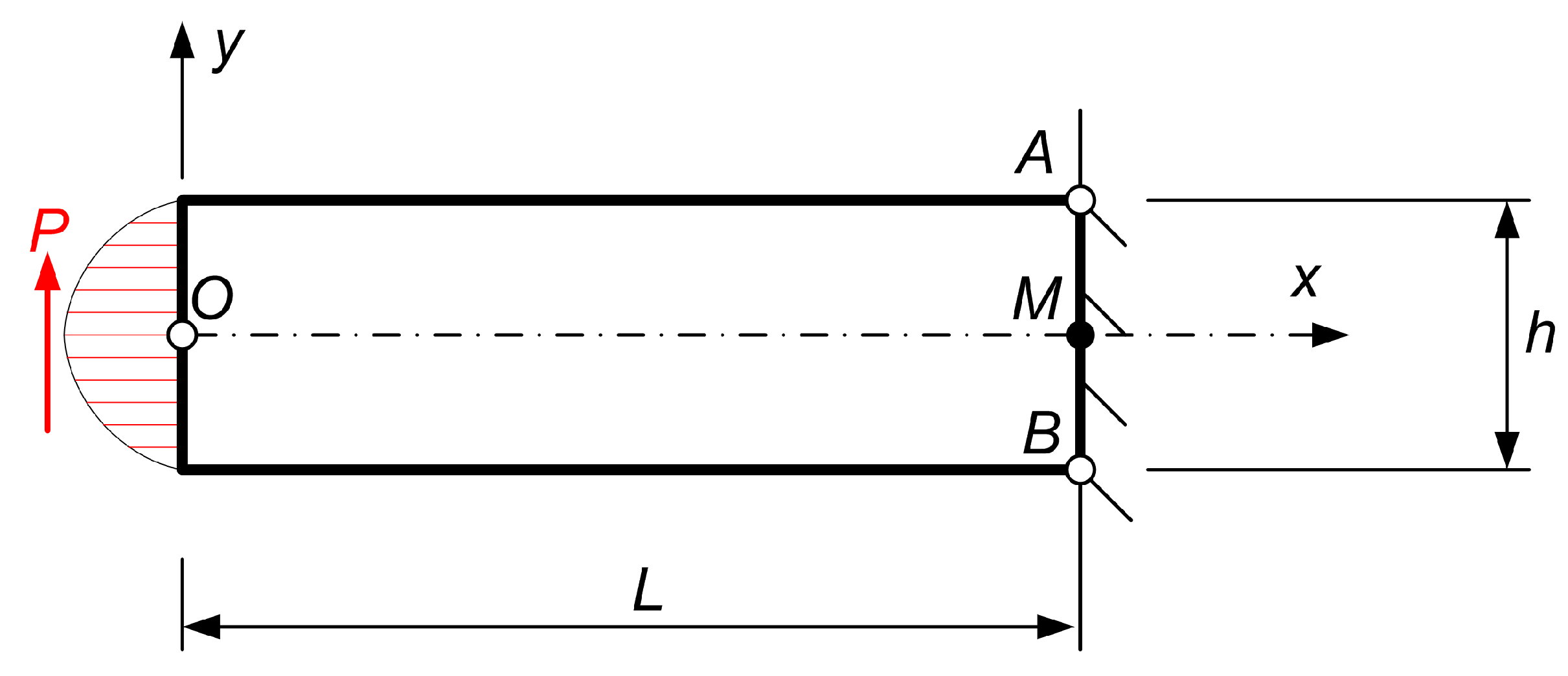
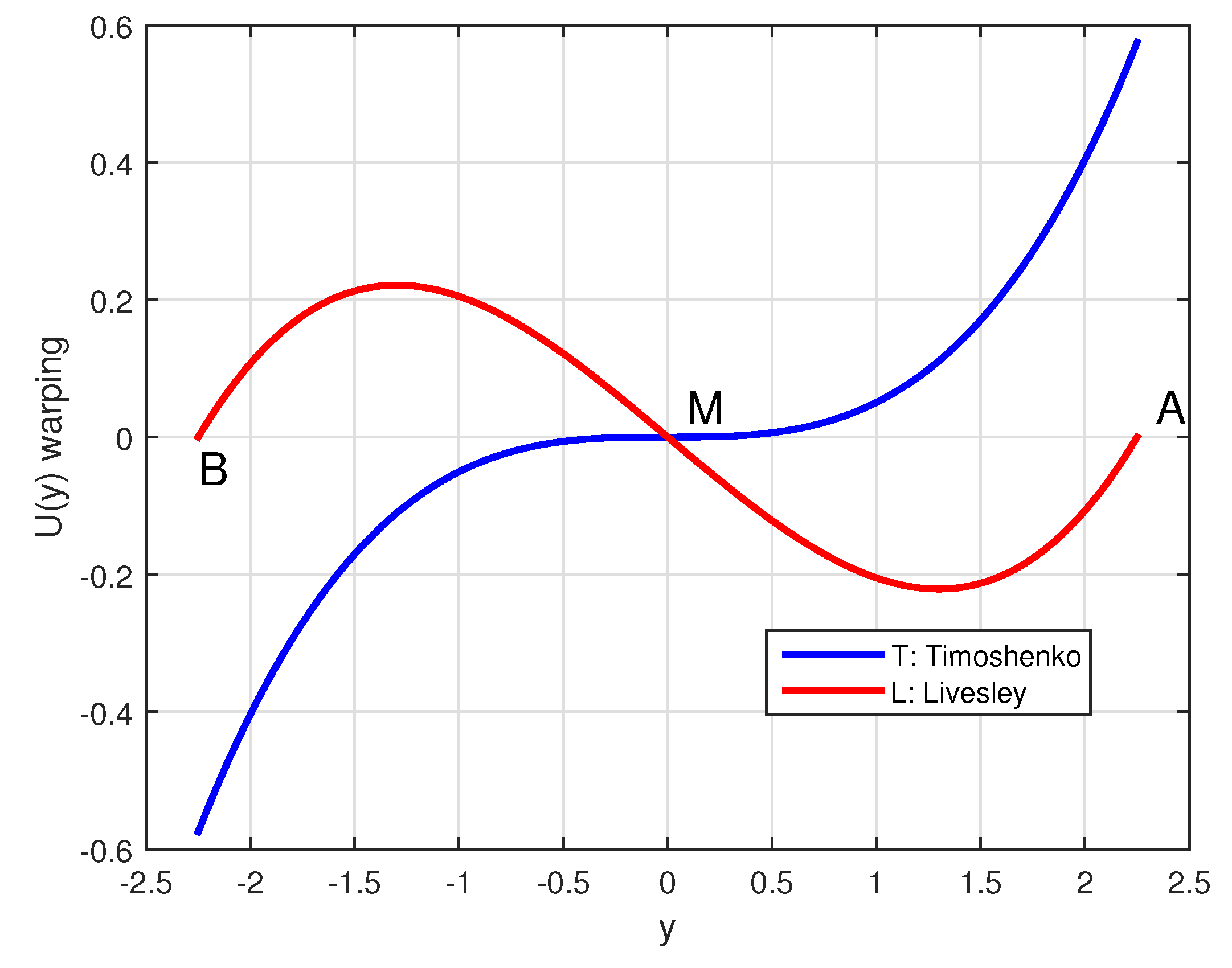
Figure 3.
Shear deflection using all the four models ().
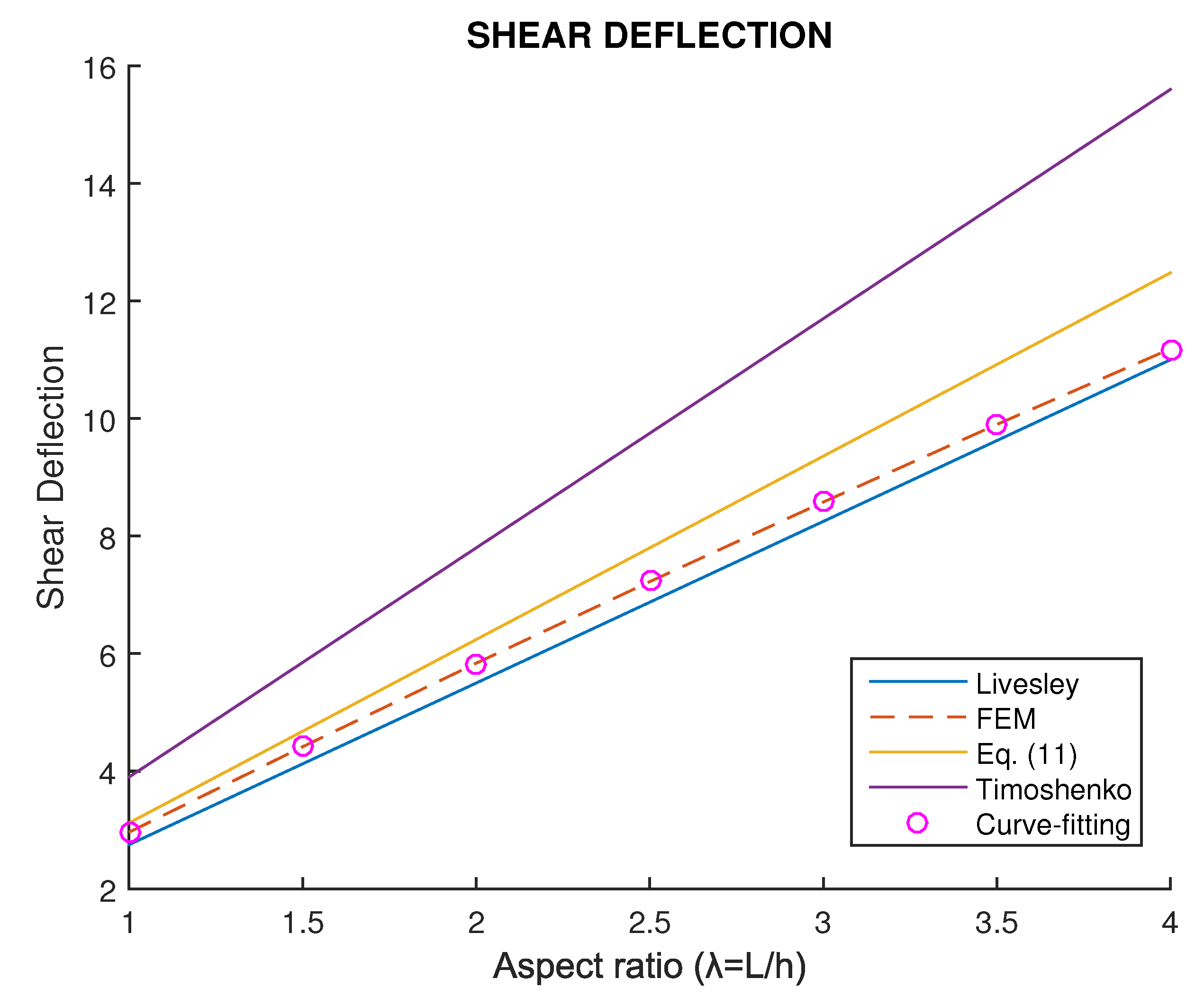
Figure 4.
FEM calculations versus analytical models for several Poisson’s ratios: (a) . (b) . (c) . (d) .
Figure 4.
FEM calculations versus analytical models for several Poisson’s ratios: (a) . (b) . (c) . (d) .
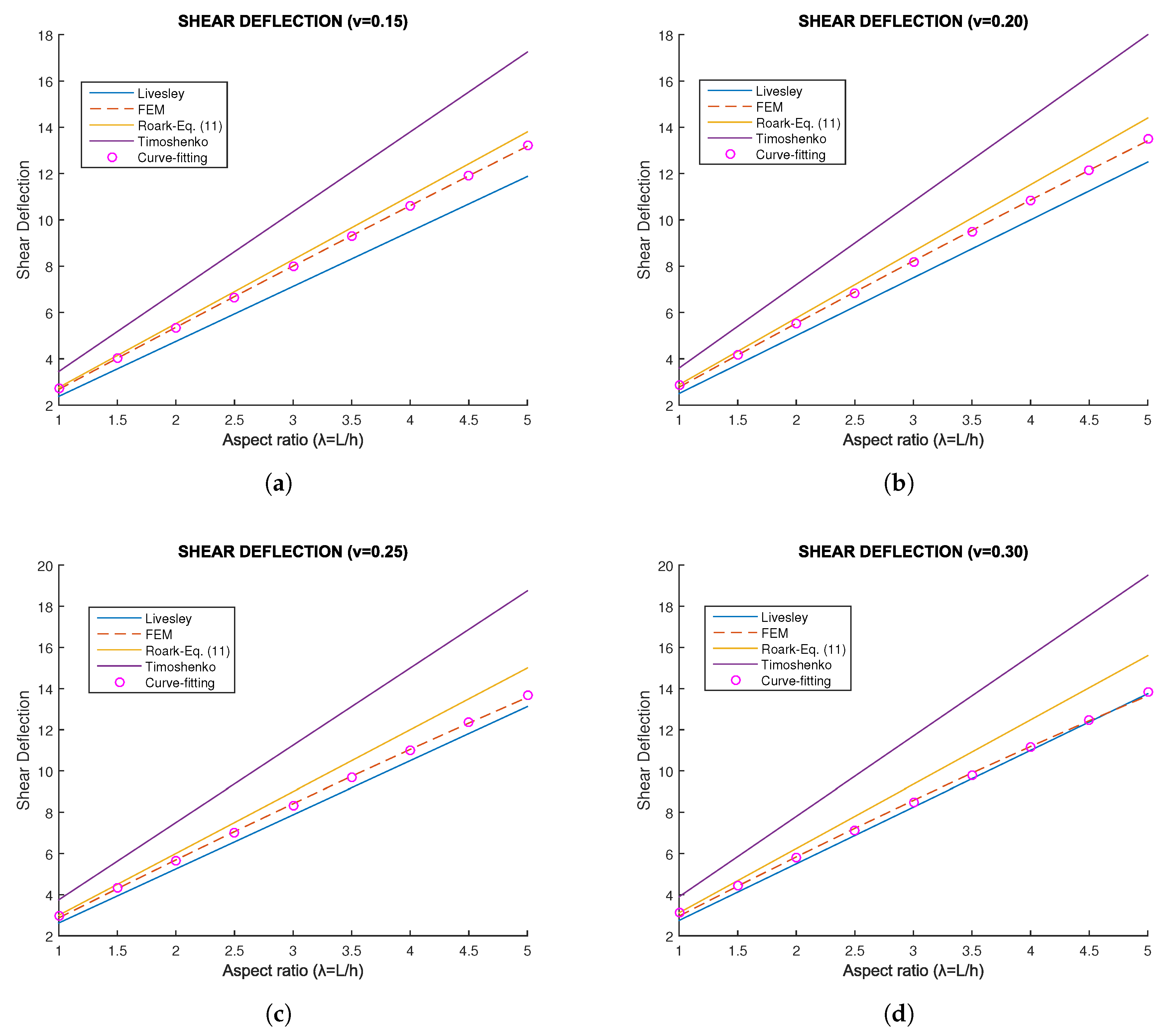
Figure 5.
Shear deflection calculated using FEM, for several Poisson ratios ().
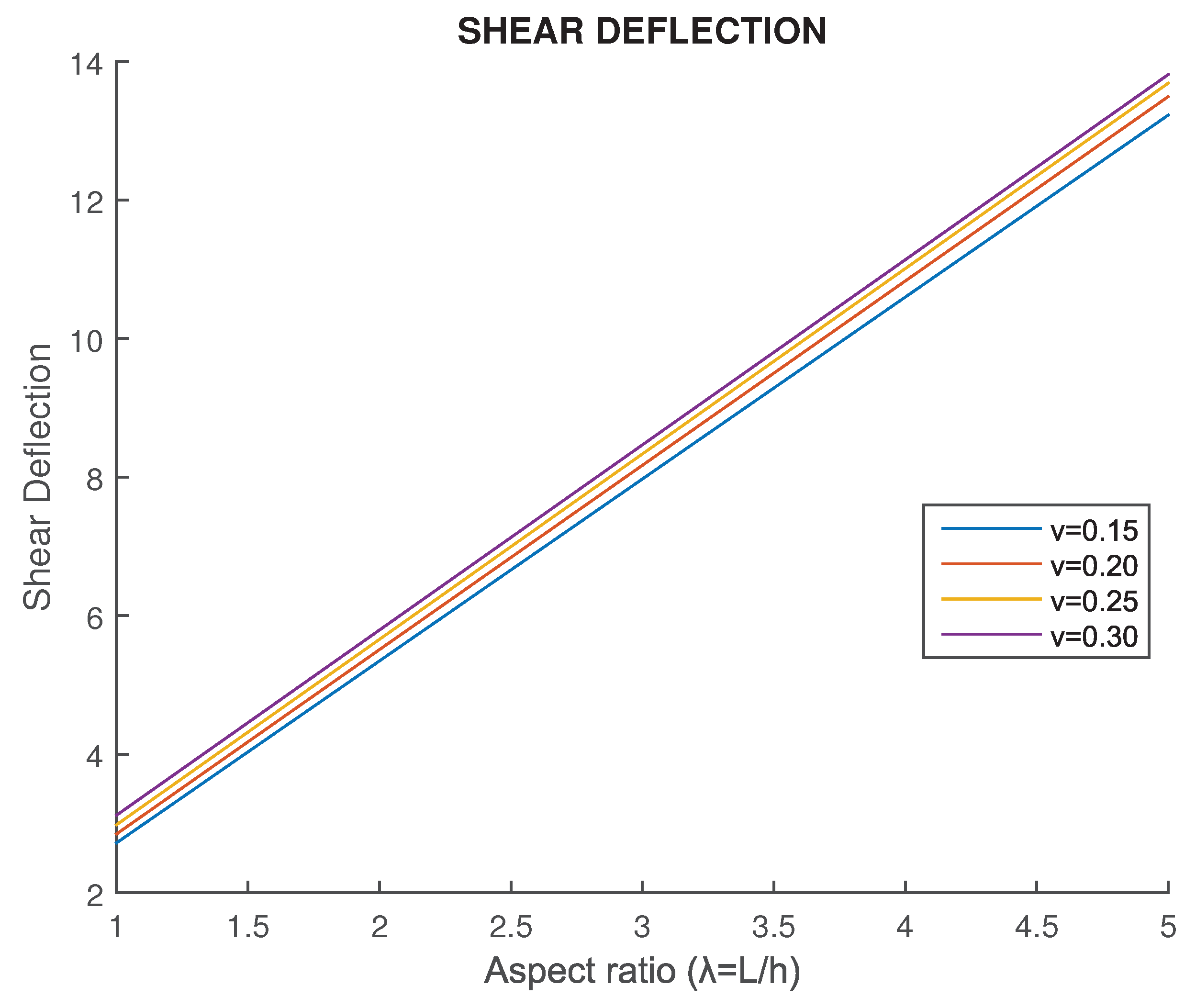
Figure 6.
Left and right limits in terms of Poisson ratio ().
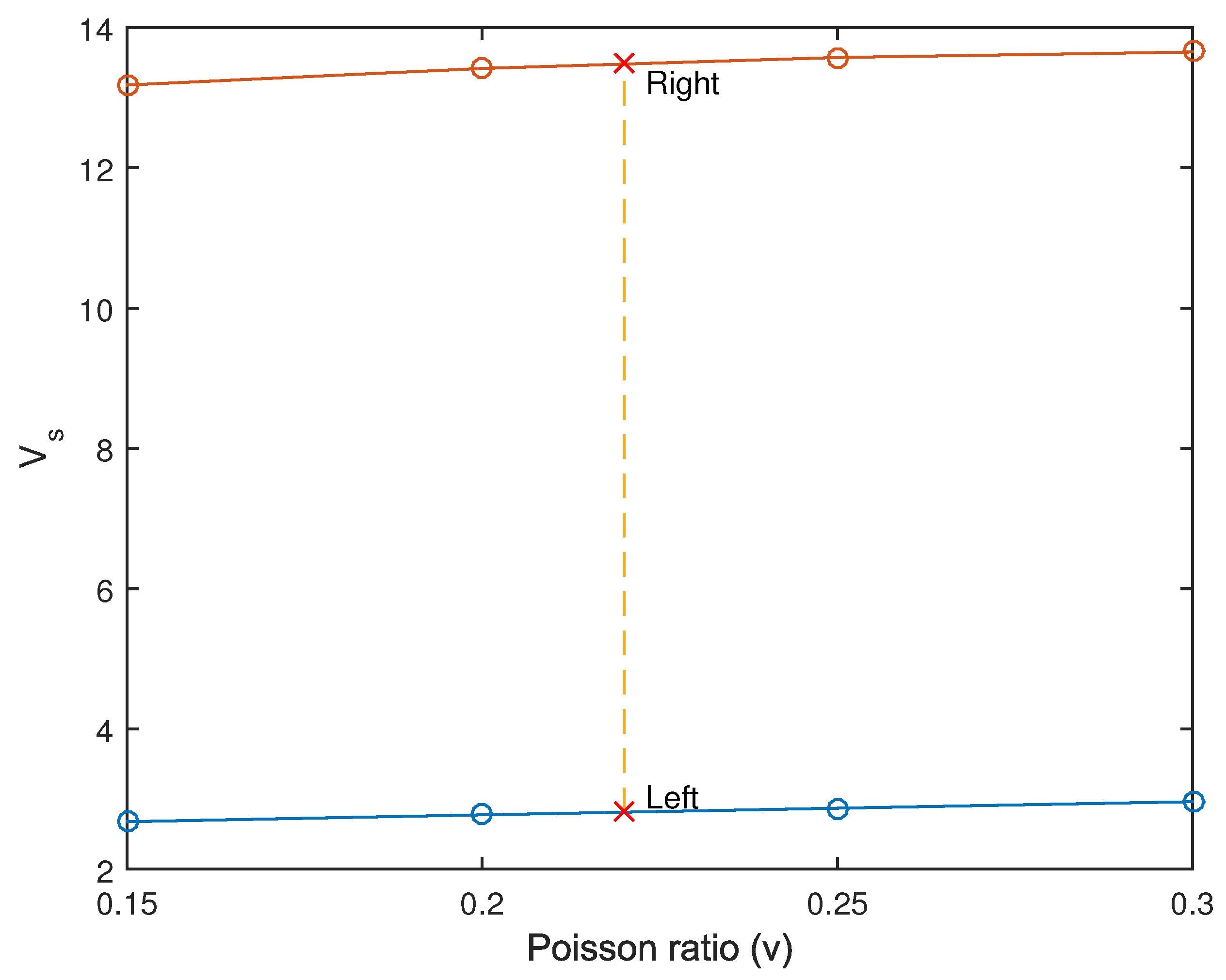

Table 1.
Constants for the prevention of rigid-body motion.
| Author | Boundary conditions | |||
|---|---|---|---|---|
| Timoshenko & Goodier [16] |
, , |
0 | ||
| Livesley [18] |
, , |
0 |
Table 2.
Total maximum deflection (for ).
| Model | |||||||
|---|---|---|---|---|---|---|---|
| Livesley | 6.7500 | 17.6250 | 37.5000 | 69.3750 | 116.2500 | 181.1250 | 267.0000 |
| FEM | 6.9618 | 17.9159 | 37.8368 | 69.7246 | 116.5790 | 181.3996 | 267.1856 |
| Roark | 7.1200 | 18.1800 | 38.2400 | 70.3000 | 117.3600 | 182.4200 | 268.4800 |
| Timoshenko | 7.9000 | 19.3500 | 39.8000 | 72.2500 | 119.700 | 185.1500 | 271.6000 |
Table 3.
Linear regression for the shear deflection , based on FEM results ().
| Poisson’s ratio () | Linear Interplation | R-squared |
|---|---|---|
| 0.15 | 0.0934210 + 2.6266105 | 0.99993159 |
| 0.20 | 0.1870982 + 2.6613086 | 0.99981251 |
| 0.25 | 0.3050623 + 2.6765495 | 0.99957846 |
| 0.30 | 0.4463497 + 2.6731285 | 0.99916785 |
| “““` |
Table 4.
Cubic regression formulas for the shear deflection , based on FEM results .
| Poisson’s ratio | Cubic interpolation formula for |
|---|---|
| 0.15 | |
| 0.20 | |
| 0.25 | |
| 0.30 |
Disclaimer/Publisher’s Note: The statements, opinions and data contained in all publications are solely those of the individual author(s) and contributor(s) and not of MDPI and/or the editor(s). MDPI and/or the editor(s) disclaim responsibility for any injury to people or property resulting from any ideas, methods, instructions or products referred to in the content. |
© 2025 by the authors. Licensee MDPI, Basel, Switzerland. This article is an open access article distributed under the terms and conditions of the Creative Commons Attribution (CC BY) license (http://creativecommons.org/licenses/by/4.0/).
Copyright: This open access article is published under a Creative Commons CC BY 4.0 license, which permit the free download, distribution, and reuse, provided that the author and preprint are cited in any reuse.


