
Submitted:
10 March 2025
Posted:
11 March 2025
You are already at the latest version
Abstract
This paper presents an analytical solution to the Levinson beam theory (LBT) for the first-order analysis of uniform beams with simple symmetrical cross-sections, contrarily to most papers on LBT that analyzed beams with rectangular or double symmetrical cross-sections. LBT is a higher-order shear deformation theory characterized by a displacement field which includes warping of the cross-section and satisfies the shear free conditions on the lower and upper surfaces of the beam. In this study, the shear stresses were assumed to have their maximal values at the centroidal axis. This led to a displacement field that was fourth-order for beams with simple symmetrical cross-sections and third-order for beams with double symmetrical cross-sections. The equilibrium equations set on a vectorial basis were composed of two coupled differential equations combining the transverse deflection and the rotation of the cross-section at the centroidal axis: after some manipulations the governing equation (a fourth-order differential equation), the efforts and deformations were expressed in terms of the transverse deflection. Finally, closed-form solutions for efforts and deformations were presented for various loading and support conditions, as well as element stiffness matrices. The results were in agreement with those in the literature for beams with rectangular cross-sections.
Keywords:
Levinson beam theory
; warping
; closed-form solutions
; element stiffness matrix
; non-uniform heating
1. Introduction
The Euler−Bernoulli Beam Theory (EBT) also called “Classical Beam Theory” is the first beam theory formulated for the analysis of beams. It was first enunciated circa 1750 and did not consider shear deformations. Therefore the deflections predicted were only accurate for slender beams: in case of short or thick beams the deflections were underestimated. To overcome the drawbacks posed by EBT a first-order shear deformation theory was proposed 1921 by Timoshenko [1]. Shear deformations were considered but shear coefficients had to be defined. Moreover, the Timoshenko beam theory predicted constant shear stresses in the cross-section, this violating the shear stress free surface conditions. To deal with the problems of the first-order shear deformation theory, higher-order shear deformation theories were developed. In this respect Levinson [2] proposed 1981 a third-order shear deformation theory for beams with rectangular cross-sections whereby the equations were derived using a vectorial formulation. The Levinson beam theory (LBT) did not use shear coefficients and the shear stress free surface condition was satisfied. The Reddy beam theory [3] proposed in 1984 used the same displacement field as LBT but the governing differential equations were based on variationnaly derived equations of equilibrium. Other research papers on shear deformation theories can be mentioned. Golbakhshi et al. [4] presented a revised couple stress model similar to the classical Timoshenko beam theory according to the third-order Reddy–Levinson beam theory. Faghidian et al. [5] conceived and applied a stationary variational framework of the Timoshenko–Ehrenfest beam, founded on the elasticity theory, to set forth the variationally consistent shear coefficient of a prismatic beam of a solid rectangular cross-section. Chen et al. [6] presented accurate values for the dynamic stiffness matrix coefficients of Levinson beams under axial loading embedded in a Winkler–Pasternak elastic foundation, while Ike [7] presented the determination of natural transverse vibration frequencies of Euler-Bernoulli beams on Winkler foundations using the Generalized Integral Transform Method. Schoeftner [8] proposed an analytical refined beam model taking into account the axial, the shear and the transverse normal stress distributions whereas Karttunen et al. [9] provided a consistent variational formulation for the static Levinson beam theory. The variational formulation was carried out by employing the principle of virtual displacements whereby the external virtual work done by the stresses on the end surfaces of the beam was included in the formulation.
In this paper the shear stresses/strains that satisfied the shear stress free surface conditions were assumed to have their maximal values at the centroidal axis. This led to a displacement field that was fourth-order for beams with simple symmetrical cross-sections and third-order for beams with double symmetrical cross-sections. The equilibrium equations set on the basis of a vectorial approach led to the formulation of the governing equation (a fourth-order differential equation), efforts and deformations in terms of the transverse deflection. So closed-form solutions for efforts and deformations could be derived for various loading and support conditions, as well as element stiffness matrices.
2. Materials and Methods
2.1. First-Order Analysis of the Levinson Beam
The sign convention adopted for the loads, bending moments, shear forces, and displacements is illustrated in Figure 1
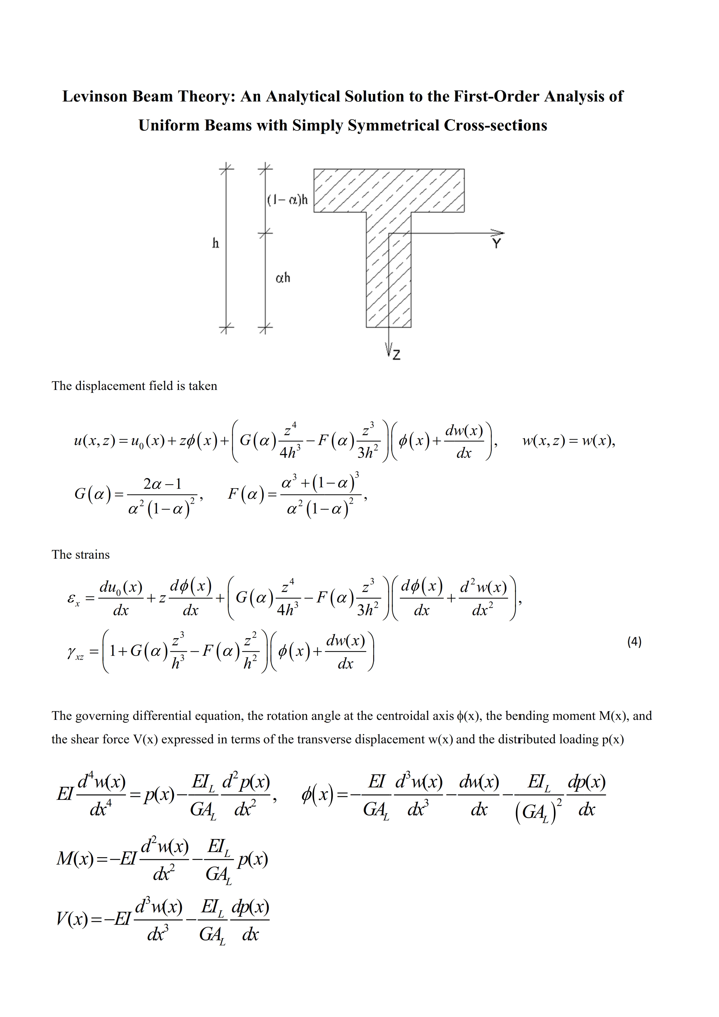
Let the displacements in x-, y-, and z- directions be denoted by u(x,y,z), v(x,y,z), and w(x,y,z), respectively. Observing the symmetry of the cross-section with respect to the z-axis, these displacements can be described as follows
The kinematic and constitutive relations are
respectively, where E and G are the Young’s modulus and the shear modulus, respectively.
In the Levinson Beam Theory (LBT), the displacement field is such that the shear stresses/strains vanish on the upper and lower surfaces of the beam. In addition, it is assumed in this study that the maximal shear stresses/strains appear in the centroidal axis.
Letting the height of the beam be h, and the z coordinates of the lower and upper surface be zl = αh and zu = - (1 - α) h, respectively, the displacement field can then be taken
where u0(x) is the displacement of the centroidal axis and φ(x) is the counterclockwise positive rotation of the cross-section at the centroidal axis. It is noted that for beams with double symmetrical cross sections α = 0.5 and the coefficients G(α) = 0, F(α) = 4, and so Equation (3) corresponds to the Levinson [2] solution for beams of rectangular cross sections. It follows the strains using Equation (2)
The bending moment M(x), shear force V(x) and axial force N(x) are calculated using Equation (2) and (4) as follows
where A and I are the area and the second moment of area of the cross-section, respectively, and I3, I4, and I5 are defined as In = ∫zndA with n = 3, 4, and 5. Let the following cross sectional values be
Deriving both sides of Equation (5b) with respect to x and combining with (6b) yields
Substituting Equation (7a) and (6a) into (5a) yields
Equation (7b) can be reformulated as follows to represent a moment − shear force − curvature relationship
In the case of non-uniform heating, Equation (7c) becomes
where αT is the coefficient of thermal expansion, ΔT = ΔTls - ΔTus is the difference between the temperature changes at lower surface (ΔTls) and upper surface (ΔTus) of the beam, and h is as before the height of the beam.
The static equilibrium equations in first-order analysis are given by
Equation (8a-c) are developed as follows using Equation (5a-c) and (6a-c)
Let us formulate Equation (8e-f) for beams with rectangular cross-sections. Recalling that G(α) = 0 and F(α) = 4
Equation (8e-f) become
Equation (8h-i) are the equilibrium equations derived by Levinson [2]. The bending moment can generally be expressed in terms of w(x) using Equation (7b) and (8b)
The shear force can also be expressed in terms of w(x) using Equation (8c) and (9)
Combining Equation (5b), (6b) and (10) yields
Combining Equation (8b-c) and (9) yields the governing differential equation of the uniform Levinson beam with simply symmetrical cross section
The governing differential equation (Equation 12), the bending moment M (Equation 9), the shear force V (Equation 10), and the rotation of the cross section (Equation 11) are expressed in terms of w(x): the analytical solution can then be found.
For illustration we consider a beam of length l carrying a uniformly distributed load p. The transverse deflection w(x) can be expressed as follows using Equation (12)
It follows the bending moment, the shear force V, and the rotation of the cross section
where λL is a bending shear factor. The integration constants C1, C2, C3, and C4 are then determined applying the boundary conditions expressed using Equation (13) and (14a-d). Results for some cases are presented in Appendix A.
It is noted that w(x) and φ(x) are determined independently from u0(x). The latter is found from the following governing equation (8d) using (8e)
and the boundary conditions involving the axial force N(x) and u0(x) at the beam’s ends.
Table 1 summarizes the Euler–Bernoulli beam equations, Timoshenko beam equations, and Levinson beam equations in terms of the transverse deflection w(x), whereby the rotation of cross-sections is counterclockwise positive and the Timoshenko shear coefficient is κ.
2.2. Stresses in the Cross-Section
In this section the stresses within the cross-section are expressed in terms of the axial force, the shear force, and the bending moment. They are calculated using Equation (2), (4), and (8e)
Substituting Equation (6c) and (8e) into (5c) yields
Equation (5a) can be reformulated as follows using (6a) and (8e) while (5b) is recalled using (6b)
From the equations above and reminding that E = 2G(1 + ν) it yields
In case of doubly symmetrical cross-sections G(α) = 0, F(α) = 4, SL = 0, IL = I – 4I4/3h2, AL = A – 4I/h2. Recalling that I4 = ∫z4dA Equation (18a-b) become
2.3. Element Stiffness Matrix
The sign convention for bending moments, shear forces, displacements, and rotation angles adopted for determining the element stiffness matrix in local coordinates is illustrated in Figure 2.
Let us define the element-end force vector and the element-end displacement vector as follows
The element stiffness matrix in local coordinates of the Levinson beam is denoted by KLl. The relationship between the aforementioned vectors is as follows:
Applying Equation (14a-d) with the distributed load p = 0 yields the following
Considering the sign conventions adopted for bending moments and shear forces in general (see Figure 1) and for bending moments and shear forces in the element stiffness matrix (see Figure 2), we can set following static compatibility boundary conditions in combination with Equation (21a-d)
Considering the sign conventions adopted for the displacements (see Figure 1) and rotations (counterclockwise positive) on the one hand and for displacements and rotations in the member stiffness matrix (see Figure 2) on the other hand, we can set following geometric compatibility boundary conditions in combination with Equation (21a-d)
Combining Equation (20), (22a-d) and (23a-d) yields the 4 × 4 first-order element stiffness matrix of the Levinson beam
The development of Equation (24) yields
The element stiffness matrix (ESM) of the Levinson beam has the same formulation as that of the Timoshenko beam whereby the coefficients in the matrices are related as follows: ALΦL = κAΦT. The ESM of the Euler−Bernoulli beam is obtained by setting ΦL = 0.
Assuming the presence of a hinge at the right end, the sign convention for bending moments, shear forces, displacements, and rotations is illustrated in Figure 3.
The element-end force vector and the element-end displacement vector become
The analysis is done similarly and the 3 × 3 element stiffness matrix of the Levinson beam is then
As before the element stiffness matrix of the Levinson beam has the same formulation as that of the Timoshenko beam whereby the coefficients in the matrices are related as follows: ALλL = κAλT.
2.4. Strong and Weak Formulation of the Boundary Conditions
The analytical solution presented in this paper satisfies the boundary conditions (BC’s) through the stress resultants (axial force, shear force and bending moment) and the rotation of cross-section only at the centroidal axis: this represents a weak formulation of the BC’s. Strong formulations of the BC’s expressed in terms of stresses and displacements are listed below for different edge conditions whereby the displacement component u0(x) is ignored since it does not contribute to M(x) and V(x).
Clamped Edge
From the strong formulation the displacements u(x, z) and w(x) are zero at any position z. From Equation (3) it yields φ = 0, dw/dx = 0, w = 0. Consequently the shear stresses and the shear force vanish regarding Equation (4) and (5b), this representing an inconsistency. By applying a weak formulation of the BC’s (φ = 0, w = 0) this inconsistency disappears.
Free Edge
The strong formulation implies the normal and shear stresses σ and τ are zero at any position z. Equation (15a-b) yields dφ/dx = 0, p(x) = 0, φ + dw/dx = 0. Hence, the absence of distributed loading is a condition for the satisfaction in a strong sense of the BC’s. The weak formulation is M = 0, V = 0.
Simply Supported Edge
From the strong formulation the normal stresses σ = 0 and the transverse deflection w = 0 at any position z. Equation (15a-b) implies dφ/dx = 0, p(x) = 0, w = 0. The absence of distributed loading is a condition for the satisfaction in a strong sense of the BC’s. The weak formulation is M = 0, w = 0.
In summary, on the one hand it is observed that the strong formulation of the BC’s is characterized with three conditions: this required a beam model described with a sixth-order governing differential equation. On the other hand the weak formulation is characterized with two conditions at each edge, which is consistent with the fourth-order governing differential equation of the Levinson beam model.
2.5. Inconsistencies in the Determination of Shear Stresses
In this study the shear stresses were determined using the stress-strain relationship or constitutive law (Equation (2d)). However they can be calculated using the equilibrium-method as it is done in the Euler−Bernoulli beam theory. Here a beam element obtained by performing plane cuts at x, x + dx, and z is considered. The equilibrium equation in x direction is set on this element using Equation (15a-b) for stresses, i.e., the shear stresses τzx = τxz have to balance-out the variation of the axial force apart from z as follows
The term on the right-hand side of Equation (28) is a fifth-order polynomial with respect to z while τxz (Equation (15b)) is a third-order polynomial with respect to z.
Therefore, similarly to Euler−Bernoulli beam theory and Timoshenko beam theory, an inconsistency remains between the shear stresses that are obtained based on the equilibrium-method and the shear stresses obtained by the constitutive law.
3. Results and Discussion
3.1. Beams with Rectangular Cross-Section
Normal and Shear Stresses
Equation (18c-d) presented the stresses for doubly symmetrical cross-sections. For rectangular cross-sections AL = 2/3A and I4 = bh5/80 were calculated in Equation (8g): it follows the stresses
These results correspond to those obtained by Karttunen [9]
Element Stiffness Matrix
Equation (25) presented the 4 × 4 element stiffness matrix with the parameter ΦL = 12λL. For rectangular cross-section
This result corresponds to that obtained by Karttunen [9]
Deflection Curve of Beam of Length 2l Simply Supported at Both Ends
A beam of uniform cross-section and length 2l simply supported at both ends and carrying a uniformly distributed load p is considered. The deflection curve is to determine whereby the origin is taken at the middle for comparison purpose with Levinson [2]. The boundary conditions are M(±l) = 0 and w(±l) = 0 at both ends while the expressions of M(x) and w(x) were given in Equation (13) and (14a).
The solution for the deflection curve of a beam of length 2l with an arbitrary simply symmetrical cross-section is
For a beam of length 2l having a rectangular cross-section Equation (8g) yields IL = 4/5I and
This result corresponds to that obtained by Levinson [2]
4. Conclusions
The Levinson beam theory (LBT) is treated by many authors for beams with rectangular cross-sections. In this paper LBT was extended to simple symmetrical beams. A displacement field which includes warping of the cross-section and satisfies the shear free conditions on the lower and upper surfaces was presented and two coupled differential equations combining the transverse deflection and the rotation of the cross-section at the centroidal axis were derived. The analysis was simplified by the formulation of the governing equation, the efforts and deformations in terms of the transverse deflection and so closed-form solutions were presented for various loading and support conditions, as well as element stiffness matrices. It was shown that a strong formulation of the boundary conditions (stress and displacement related) presented many inconsistencies while the weak formulation (related to the efforts and the rotation of the cross-section at the centroidal axis) utilized in this study gave results that were in agreement with those in the literature for beams with rectangular cross-sections. However, an inconsistency remained between the shear stresses that are obtained based on the equilibrium-method and the shear stresses obtained by the constitutive law.
The following aspects of LBT not addressed in this study could be examined in future research:
- ✓ Second-order analysis of beams
- ✓ Buckling analysis of beams
- ✓ Vibration analysis of beams
Conflicts of Interest
The author declares no conflict of interest.
Appendix A. Closed-Form Expressions of Single-Span Systems for Various Support Conditions and Loadings
The beams (0 ≤ x ≤ l) are of length l. The equations of Section 2.1 are applied, together with the corresponding weak forms of the boundary conditions. The uniformly distributed loading, triangular distributed loading and the non-uniform heating are considered. The efforts and deformations for uniformly distributed loading presented in Equations (13) and (14a-d) are recalled below, and they are as follows for triangular distributed loading and non-uniform heating
Uniformly distributed load p
Triangular distributed load (zero at x = 0, and p at x = l)
Non-uniform heating
Equation (7d) is applied with dV(x)/dx = 0
The integration constants C1, C2, C3, and C4 are determined using the boundary conditions.
The closed-form expressions of bending moment and deflection curves are presented below, with another bending shear factor αL and a thermal curvature strain κT defined as follows
Pinned–pinned beam
- Uniformly distributed load p
- Triangular distributed load (zero at x = 0, and p at x = l)
- Non-uniform heating
Fixed–Free beam (clamped edge at x = 0)
- Uniformly distributed load p
- Triangular distributed load (zero at x = 0, and p at x = l)
- Non-uniform heating
Fixed–pinned (clamped edge at x = 0)
- Uniformly distributed load p
- Triangular distributed load (zero at x = 0, and p at x = l)
- ∙ Non-uniform heating
Fixed–fixed beam
- Uniformly distributed load p
- Triangular distributed load (zero at x = 0, and p at x = l)
- Non-uniform heating
Appendix B. Levinson Beam Subjected to a Concentrated Load P and an External Bending Moment M*
Given a beam of length l subjected to a concentrated load P and an external moment M*(counterclockwise) applied at a distance a from the left-hand end. Equation (13) and (14) with p = 0 are applied as follows on both sides of the concentrated loads, x1 at the left side (0 ≤ x1 ≤ a) and x2 at the right side (0 ≤ x2 ≤ b):
Similar equations are applied on the right side (with the variable x2 and the integration constants B1, B2, B3, and B4 as follows
The analysis is conducted for different beam support conditions.
Fixed − pinned beam
Following boundary conditions and continuity conditions are set:
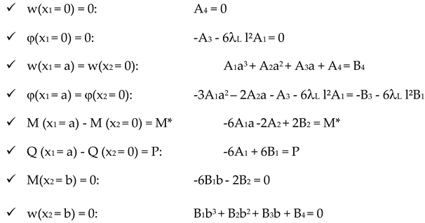
The integration constants A1, A2, A3, A4, B1, B2, B3, and B4 are determined by solving the above system of equations and are given by
The efforts and displacements are then calculated using Equation (B1a-b).
Fixed − fixed beam
The continuity equations are the same with Equation (B3). The integration constants are given by
Fixed − free beam
Pinned − pinned beam
References
- Timoshenko, S. P. On the Correction for Shear of the Differential Equation for Transverse Vibrations of Prismatic Bars. Philos Mag, Vol. 41, pp. 744_746, 1921.
- Levinson, M. A New Rectangular Beam Theory. J Sound Vib, Vol. 74, pp. 81–87, 1981.
- Reddy, J. N. A Simple Higher-Order Theory for Laminated Composite Plates. J. Appl. Mech. 51 (4) (1984) 745_752.
- Golbakhshi, H., Dashtbayazi M. R., Saidi A. R. A New Theoretical Framework for Couple Stress Analysis of Reddy–Levinson Micro-Beams. International Journal of Applied Mechanics Vol. 14, No. 07, 2250069 (2022). [CrossRef]
- Faghidian, S.A., Elishakoff, I. The Tale of Shear Coefficients in Timoshenko–Ehrenfest Beam Theory: 130 Years of Progress. Meccanica 58, 97–108 (2023). [CrossRef]
- Chen, Z., Cheng, Q., Jin, X., Borodich, F. M. (2024). Dynamic Stiffness for a Levinson Beam Embedded Within a Pasternak Medium Subjected to Axial Load at Both Ends. Buildings, 14(12), 4008. [CrossRef]
- Ike, C.C. Free Vibration of Thin Beams on Winkler Foundations Using Generalized Integral Transform Method. Engineering and Technology Journal 41 (11) (2023) 1286 – 1297. http://doi.org/10.30684/etj.2023.140343.1462.
- Schoeftner, J. An Accurate and Refined Beam Model Fulfilling the Shear and the Normal Stress Traction Condition. International Journal of Solids and Structures, Volume 243, 2022, 111535, ISSN 0020-7683. [CrossRef]
- Karttunen, A. T., v H, Raimo. Variational Formulation of the Static Levinson Beam Theory. Mech. Res. Commun. 2015;66:15. [CrossRef]
Figure 1.
Sign convention for loads, bending moments, shear forces, and displacements.
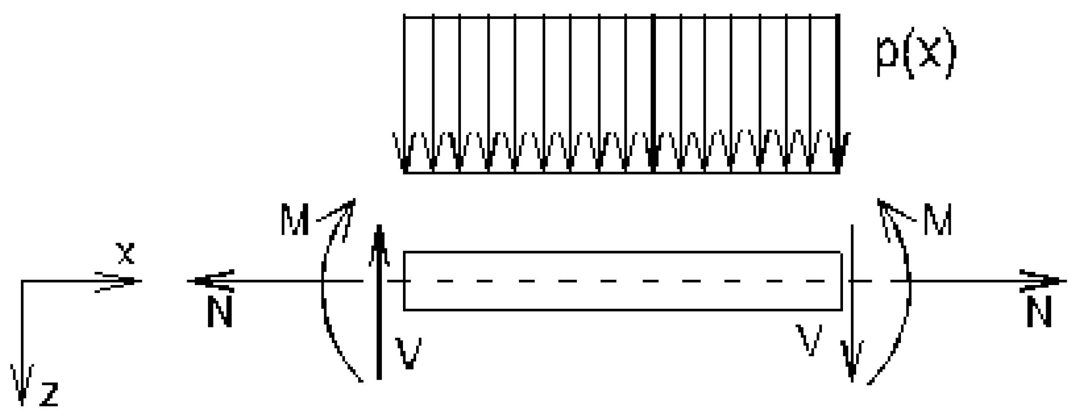
Figure 2.
Sign convention for moments, shear forces, displacements, and rotation angles for stiffness matrix.
Figure 2.
Sign convention for moments, shear forces, displacements, and rotation angles for stiffness matrix.
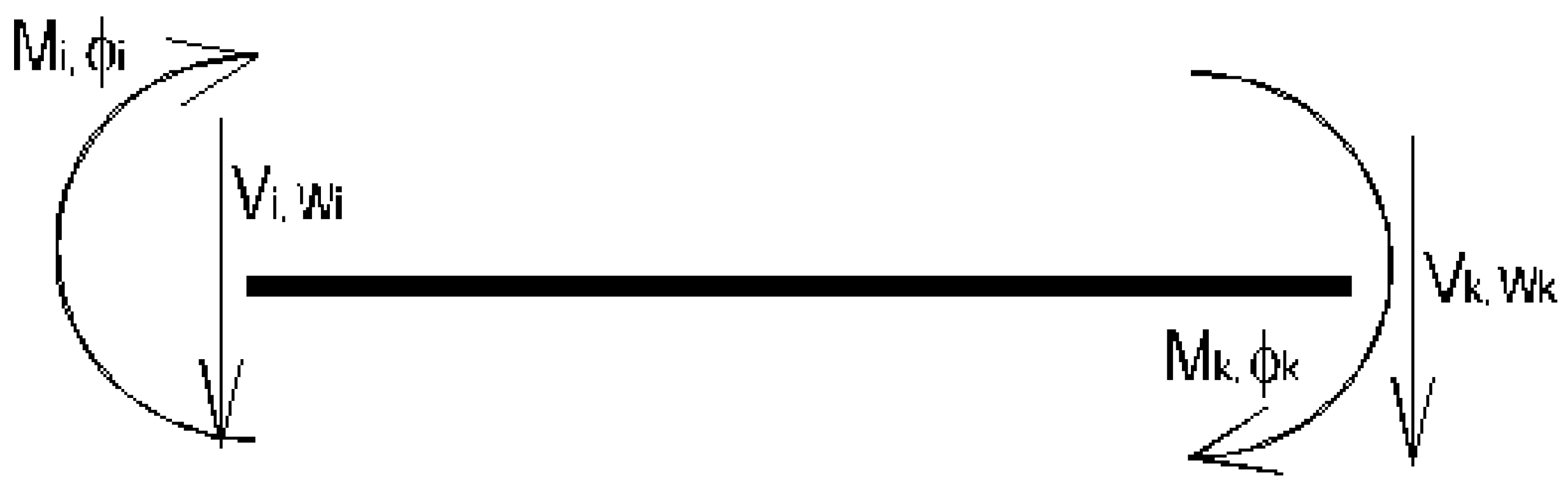
Figure 3.
Sign conventions for moments, shear forces, displacements, and rotations for stiffness matrix.
Figure 3.
Sign conventions for moments, shear forces, displacements, and rotations for stiffness matrix.
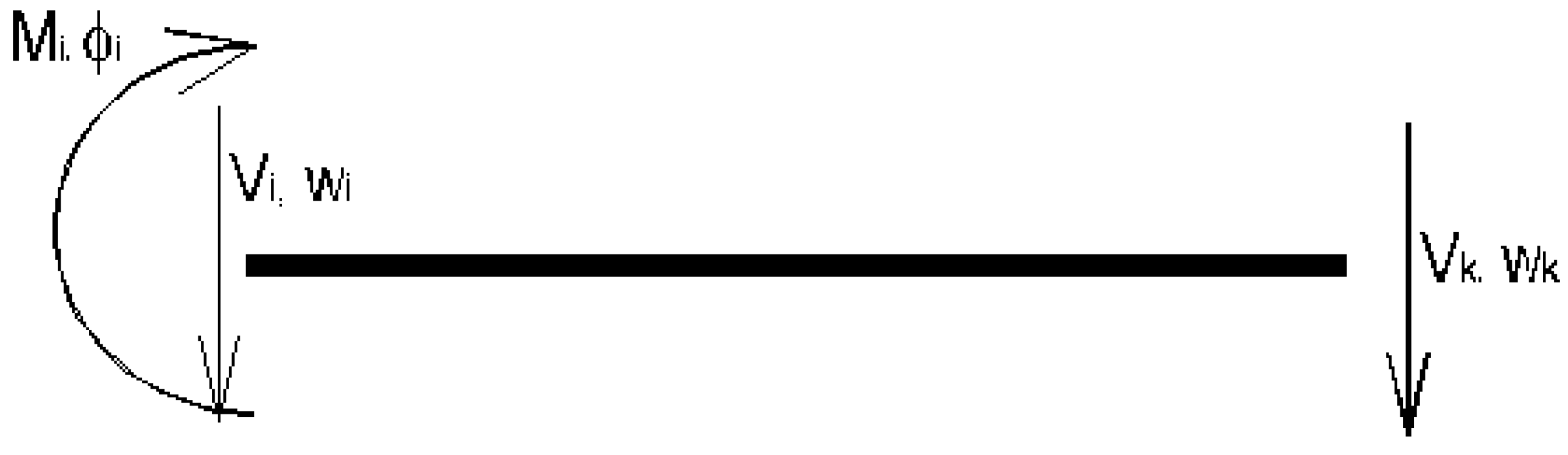

Table 1.
Summary of equations for Timoshenko and Euler–Bernoulli beams.
| Euler–Bernoulli beam | Timoshenko beam | Levinson beam | |
| Governing differential equation | |||
| Rotation of cross section | |||
| Bending Moment | |||
| Shear force |
Disclaimer/Publisher’s Note: The statements, opinions and data contained in all publications are solely those of the individual author(s) and contributor(s) and not of MDPI and/or the editor(s). MDPI and/or the editor(s) disclaim responsibility for any injury to people or property resulting from any ideas, methods, instructions or products referred to in the content. |
© 2025 by the authors. Licensee MDPI, Basel, Switzerland. This article is an open access article distributed under the terms and conditions of the Creative Commons Attribution (CC BY) license (http://creativecommons.org/licenses/by/4.0/).
Copyright: This open access article is published under a Creative Commons CC BY 4.0 license, which permit the free download, distribution, and reuse, provided that the author and preprint are cited in any reuse.


