
Submitted:
28 July 2025
Posted:
29 July 2025
You are already at the latest version
Abstract
This paper investigates the Heterogeneous Electric Vehicle Routing Problem with Time Windows and Energy Minimization, a critical challenge in sustainable urban logistics. We propose a Mixed-Integer Linear Programming model that explicitly minimizes the total energy consumption of a heterogeneous electric vehicle (EV) fleet while satisfying customer demands within specific time windows. The model accounts for vehicle diversity in terms of battery capacities, consumption rates, and charging characteristics, and incorporates distance- and load-based energy consumption under a full-recharge policy. Computational experiments are conducted on a comprehensive set of benchmark-based instances. Results demonstrate the model’s ability to find optimal or near-optimal solutions for small-scale problems, with acceptable optimality gaps for larger instances. Sensitivity analyses reveal the influence of key parameters—battery capacity ratios, consumption rates, recharging speeds, maximum number of active EVs, and payload sensitivity—on energy usage and fleet configuration. Notably, increasing battery capacity or fleet size significantly reduces energy consumption up to a saturation point, while inefficient or slow-charging vehicles negatively affect performance. The findings have direct implications for logistics operators seeking to enhance energy efficiency and environmental performance in EV-based delivery systems.
Keywords:
electric vehicle routing
; heterogeneous fleet
; energy minimization
; time windows
; mixed-integer linear programming
; sustainable logistics
1. Introduction
Electric Vehicles (EVs) are increasingly becoming a vital component of modern transportation systems due to their potential to reduce greenhouse gas emissions, lower operating costs, and promote sustainable urban logistics [1]. In recent years, the deployment of EVs has expanded beyond personal transportation to include public transit, freight distribution, and last-mile delivery services [2,3]. Their adoption in logistics operations is particularly significant in urban environments, where strict emissions regulations and growing concerns over environmental impact are driving a shift away from traditional Internal Combustion Engine (ICE) vehicles.
Among the key challenges in utilizing EVs for logistics is the effective planning of their routes, especially considering their limited battery capacities, varying energy consumption rates, and recharging requirements. This has led to the development of specialized routing problems tailored to electric vehicles, broadly called the Electric Vehicle Routing Problem (EVRP) [4,5]. A particularly relevant variant in real-world applications is the Heterogeneous Electric Vehicle Routing Problem with Time Windows (HEVRP-TW) [6,7,8], where the fleet consists of multiple types of EVs with differing capacities, speeds, and energy efficiencies, and where customers must be serviced within specified time windows.
Incorporating energy minimization into vehicle routing decisions is critical for logistics providers aiming to enhance environmental sustainability and operational efficiency [9,10]. Unlike traditional cost-based routing objectives, minimizing the total energy a fleet consumes directly aligns with sustainability goals. Energy-aware routing mitigates the environmental impact of logistics and addresses infrastructure constraints such as limited charging station availability [11].
This paper addresses the Heterogeneous Electric Vehicle Routing Problem with Time Windows and Energy Minimization (HEVRP-TW-EM), where the primary objective is to minimize the total energy consumption of a heterogeneous fleet of EVs while ensuring that all customer demands are met within their respective time windows. We propose a detailed Mixed-Integer Linear Programming (MILP) formulation that captures key elements such as vehicle heterogeneity, time constraints, battery limitations, and energy consumption based on vehicle load and distance traveled. We comprehensively analyze various scenarios and parameter configurations to provide insights into theoretical model performance and practical applicability.
The remainder of the paper is organized as follows: Section 2 reviews the relevant literature on HEVRP-TW and energy-efficient logistics. Section 3 formally defines the HEVRP-TW-EM and presents the proposed MILP model. Section 4 discusses the computational experiments and results. Finally, Section 5 concludes the paper and offers directions for future research.
2. Related Works
A crucial variant of the EVRPs is the HEVRP-TW, which considers realistic operational constraints such as fleet heterogeneity and customer service time windows. Next, we review recent contributions that address this problem.
Kinanti et al. [12] introduced an HEVRP with soft time windows and variable energy consumption based on load and distance. They proposed an MILP and employed the Adaptive Large Neighborhood Search (ALNS) to handle large instances, highlighting the trade-offs between energy cost and service quality. Also, Hiermann et al. [6] formulated the Electric Fleet Size and Mix Vehicle Routing Problem with Time Windows and Recharging Stations (E-FSMVRPTW), integrating vehicle acquisition decisions and partial recharging. Their two-index MILP model incorporates detailed vehicle energy consumption and uses a variable neighborhood search for solving realistic-sized instances.
Penna et al. [7] proposed a hybrid Iterated Local Search (ILS) metaheuristic for the E-FSMVRPTW. Their algorithm improves efficiency and solution quality by integrating destroy-repair operators and a customized local search, showing better scalability for large instances. Li et al. [13] extended the HEVRP-TW to include simultaneous pickup and delivery operations. Their MILP formulation addresses vehicle heterogeneity, energy limits, and recharging constraints. To enhance computational performance, a hybrid decomposition-based heuristic was proposed. Zhou et al. [14] considered vehicle recycling and partial recharging in formulating an extended EVRP with time windows. Their multi-compartment energy model allows vehicles to recharge partially at stations, enabling energy-efficient routing and service continuity.
Moreover, Zhao et al. [15] introduced a bi-objective HEVRP-TW with a mixed fleet, minimizing total cost and tardiness. A modified NSGA-II metaheuristic was developed to generate high-quality Pareto solutions while accounting for soft time windows. Daysalilar et al. [8] developed a model featuring a heterogeneous fleet, diverse charging station types, and soft time windows. Their MILP accounts for partial recharging and charger compatibility, and they solve it using a customized Adaptive Large Neighborhood Search (ALNS). Mohammadbagher and Torabi [16] formulated a multi-objective HEVRP-TW with full and partial charging decisions, load-based energy use, and recharging station selection. They proposed a MILP model and solved it with the -constraint method and ALNS for large-scale evaluation.
Furthermore, Devaux et al. [17] introduced a variant incorporating simultaneous pickup and delivery with load-dependent energy consumption. Their model incorporates heterogeneity and accounts for linear energy rates that are influenced by vehicle load. A hybrid genetic algorithm was proposed to handle the problem. Additionally, Wang and Zhao [18] proposed a recharging-aware E-FSMVRPTW that utilizes a partial linear recharging strategy. Their solution approach is a multi-start local search embedded in a tailored hybrid algorithm, enabling scalable performance with high accuracy. Mozhdehi et al. [19] presented Edge-DIRECT, a Deep Reinforcement Learning (DRL)-based method for HEVRP-TW. Their model supports charging decisions and energy constraints and learns adaptive routing policies using a graph attention network and transformer modules. Recently, Moradi et al. [20] studied the EVRP-TW with an energy minimization objective and a same-day policy. They developed a mathematical model to reduce the energy consumption and usage costs.
In addition, several studies have investigated the heterogeneous Green Vehicle Routing Problem with Time Windows (HGVRP-TW), which incorporates green vehicles. For example, Macrina et al. [21] presented a Green Mixed Fleet Vehicle Routing Problem with Partial Battery Recharging and Time Windows (GMFVRP-PRTW). The study considers a fleet of electric and internal combustion vehicles and explicitly models pollutant emissions from conventional vehicles. An MILP formulation with a tailored ILS metaheuristic is proposed to solve the model efficiently. Similarly, Macrina et al. [22] extended this work by proposing an energy-efficient green-VRP with a mixed fleet and more realistic energy consumption modeling. Their model accounts for speed, acceleration, deceleration, load, and gradient effects. Partial battery recharging is allowed at charging stations, and the problem is solved using a matheuristic embedded within a large neighborhood search framework. Also, Rezaei et al. [23] tackled an HGVRP-TW with limited vehicle numbers and filling stations. They formulated a bi-objective MILP model to minimize transportation costs and emissions. Two metaheuristics—Genetic Algorithm (GA) and Population-Based Simulated Annealing (PBSA)—were developed to solve large-scale instances.
These studies demonstrate progress in solving HEVRP-TW through diverse modeling and heuristic strategies. Most works, as given in Table 1, incorporate energy consumption models, charging constraints, and time windows; however, few directly optimize total energy consumption as the primary objective. Our study distinguishes itself by focusing on energy minimization as the main objective, modeling HEVRP-TW-EM as an MILP, and conducting parameterized scenario analysis to assess theoretical and practical performance.
3. Problem Statement
3.1. Problem Description
This study addresses HEVRP-TW-EM, a realistic extension of the HEVRP-TW tailored for sustainable urban logistics. In this problem, customer demands must be fulfilled by a fleet of EVs that differ in load capacities, battery ranges, speed, and energy consumption/recharging rates. Each customer must be served within a predefined time window, adding temporal constraints to the routing decisions. The central objective is to minimize the total energy consumed by the EV fleet during the delivery operations. To accurately represent the real-world operational setting, the model accounts for vehicle heterogeneity, distance- and load-based energy consumption, and the need for some vehicles to recharge during the route (we assume each EV visits each charging station at most once on its route with full recharge policy). Energy usage is typically a function of distance traveled and vehicle load. Additionally, routes must start and end at a central depot, and each customer is visited exactly once by a single vehicle.
In this study, the energy consumption of EVs is modeled using a formulation derived from the physical law of mechanical work, adapted to account for the influence of payload [9]. Specifically, when an EV travels from node i to node j, the energy consumed on arc , denoted , is calculated as: , where represents the distance between nodes i and j, and is the payload weight carried by the EV while traversing that arc. The term linearly scales the energy cost based on the payload, acknowledging that heavier loads result in higher energy consumption. By summing this expression over all arcs and all EVs, the total energy consumption can be incorporated into the objective function of our optimization model. The resulting objective aims to minimize energy consumed across all routes, while adhering to customer time windows, EV battery and load capacities, and service constraints.
3.2. Problem Modeling
The problem is defined on a directed graph , where V is the set of all nodes and A is the set of directed arcs connecting them. The node set V includes the central depot (node ), a set of customer nodes C, a set of charging stations F, and a dummy node representing the end of each vehicle’s route. The subset represents all intermediate service points excluding the depot. Each arc represents a possible direct route from node i to node j, where and , with the condition . Each arc has an associated travel distance and travel time , where is the speed of vehicle , the set of EVs available at the depot. Each customer has a demand that must be delivered within a predefined time window . The service time at node i is denoted by . The load capacity and battery capacity of each EV k are denoted by and , respectively. While traveling, each vehicle consumes battery energy at a rate per unit distance and may recharge at any charging station at a rate .
The model uses several decision variables to describe EVs’ routing and energy behavior. The binary variable is equal to 1 if vehicle k travels from node i to node j; otherwise, it is 0. Similarly, is equal to 1 if vehicle k serves customer i, and 0 otherwise. The variable denotes the load carried by vehicle k on arc , while tracks the remaining battery level of vehicle k upon arrival at node i. The arrival time of vehicle k at node i is given by . The model integrates routing, load, battery, and time decisions to ensure that all customers are served within their time windows, the EVs respect their load and energy limits, and the total energy consumed, which depends on distance and load, is minimized. A big-M constant is also included to linearize the time-related constraints in the MILP formulation (all notations and their definitions are given in Table 2 for readers’ convenience). The MILP model for the HEVRP-TW-EM is presented as follows:
subject to,
The objective function (1) minimizes the total energy consumption of all EVs. The energy consumed on an arc is modeled as proportional to the distance and scaled by the payload carried on that arc, thereby accounting for the influence of load on energy usage. The routing constraints begin with (2), which ensures flow conservation at all intermediate nodes: if a vehicle enters a node, it must also leave it. Constraints (3) enforce that each route must start from the central depot and return to the dummy depot. The constraint (4) limits the total number of EVs used in any feasible solution. The left-hand side counts the number of EVs departing the depot (since each active vehicle must leave the depot at least once). By ensuring this total does not exceed , we enforce an upper bound on the fleet size effectively deployed on the routes. This reflects operational policies or capacity limitations restricting the number of vehicles that can be activated, even if more vehicles are available in the fleet. Constraints (5) restrict each vehicle to exiting any charging station at most once, preventing multiple departures from the same station. Constraints (6) guarantee that each customer is visited exactly once by any one vehicle. Constraints (7) link the routing decision to the service assignment by stating that if a vehicle serves a customer, it must also leave from that customer node. Constraints (8) ensure that each vehicle can start at most one route from the depot. Load and capacity constraints are modeled in (9) to (11). Constraints (9) bound the payload carried on each arc based on the vehicle’s capacity and ensure the payload is zero if the arc is not traversed. Constraints (10) enforce flow balance for customer nodes, stating that the difference between incoming and outgoing load must equal the customer’s demand. Constraints (11) do the same for charging stations, but since they neither demand nor supply goods, the net flow must be zero. Battery constraints are represented in (12) to (14). Constraints (12) update the remaining battery level after a vehicle travels between customer nodes. Constraints (13) model the same for transitions from the depot or charging stations. Constraints (14) restrict the initial battery level at the depot to not exceed the vehicle’s maximum capacity. Time window constraints are defined in (15) to (17). Constraints (15) ensure that the vehicle arrives at the next node only after completing service and travel from the current node. Constraints (16) include recharging time at charging stations and ensure it fits within the timeline. Constraints (17) enforce that the vehicle arrives at any node within its specified time window. Finally, constraints (18) define the domains of the decision variables.
4. Computational Results
This section presents the computational experiments conducted to evaluate the proposed model. We first introduce the generated dataset (Section 4.1), which comprises problem instances of varying sizes, with the number of customer nodes ranging from 5 to 50, to reflect scenarios spanning small to large scales. The vehicle fleet comprises 50 heterogeneous vehicles, characterized by diverse capacities and operational parameters. The model was solved using the Gurobi Optimizer within a two-hour runtime limit, enabling us to obtain exact solutions and performance indicators across the different instances (Section 4.2, Section 4.3 and Section 4.4). In addition, extensive sensitivity analyses were conducted to assess the impact of key parameters, explore alternative scenarios, and gain a deeper understanding of the problem’s complexity under varying operational conditions (Section 4.5 to Section 4.6).
4.1. Dataset Generation
To evaluate the performance of the proposed HEVRP-TW-EM model, we generated a comprehensive set of problem instances adapted from benchmark EVRP-TW datasets [5]. Specifically, the classical EVRP-TW instances were modified to reflect vehicle heterogeneity and additional operational parameters relevant to the studied problem. Three groups of small-scale instances were constructed, each varying in customer set size: 12 instances with five customers, 12 instances with ten customers, and 12 instances with fifteen customers, yielding a total of 36 test cases. In all small-scale cases, the number of available EVs was set equal to the number of customers, i.e., , to ensure adequate fleet availability. Furthermore, an operational constraint was imposed to limit the maximum number of EVs allowed to be used in any solution, defined as , where denotes the number of customers. To model vehicle heterogeneity realistically, the parameters characterizing each EV were randomly generated within predefined intervals. For each EV k, the battery consumption rate per unit distance was drawn uniformly from , the recharging rate from , the battery capacity from , and the payload capacity from . This variability in vehicle attributes ensures that the instances capture diverse operational conditions, allowing for an assessment of the model’s capacity to handle heterogeneous fleets.
For the medium-scale test cases, we constructed instances with 30 customer nodes to evaluate the model’s scalability and performance under more complex conditions. These instances were generated by adapting the large-scale EVRP-TW datasets. Specifically, for each large instance, we selected the first 30 customer nodes to create consistent and comparable medium-sized problems. In these instances, the number of available EVs was set equal to the number of customers, i.e., , to ensure sufficient fleet capacity for feasible solutions. The maximum number of EVs allowed to be deployed in any solution was defined as . The vehicle-related parameters, including the battery consumption rate per distance unit , recharging rate , battery capacity , and payload capacity , were generated using the same intervals and procedures applied in the small-scale instances.
To create large-scale test cases, we selected instances with 40 customer nodes, representing the most challenging scenarios in our experimental study. These instances were derived by adapting the benchmark EVRP-TW datasets, specifically by extracting the first 40 customer nodes from each large dataset to ensure consistency with the original problem structure. As in the medium-scale instances, the number of available EVs was set equal to the number of customers, i.e., , with the maximum number of EVs allowed to be used defined as . All vehicle-related parameters, including the battery consumption rate , recharging rate , battery capacity , and payload capacity , were generated using the same parameter ranges and procedures applied to the smaller problem sizes. This approach ensures a consistent experimental framework across all scenarios, allowing for a comparative analysis of the model’s performance and computational requirements as the instance size increases. The generated datasets provide a rich testbed to analyze the model’s computational performance, including the impact of vehicle heterogeneity, battery, and capacity constraints on energy consumption and routing decisions.
4.2. Results on Small-Scale Instances
This subsection presents the computational results obtained from solving the small-scale instances of the HEVRP-TW-EM using the Gurobi solver. The result of Gurobi for these instances is presented in Table 3. These instances cover customer set sizes of , 10, and 15, amounting to a total of 36 test cases. The performance metrics reported include the best objective function value (OFV), which corresponds to the total energy consumption by the EVs (i.e., objective function (1)), the runtime in seconds, and the optimality gap achieved within the time limit of 7200 seconds. For instances with 5 customers, Gurobi solved all 12 cases to optimality. The average OFV across these cases was 4208.14, and the average runtime was relatively low at 8.41 seconds, with no instance exceeding the time limit. The optimality gap was zero for all cases. Despite the small problem size, some instances required more time due to spatial characteristics and demand distribution, such as r203C5 and c101C5, which took 32.88 and 23.86 seconds, respectively. For instances with 10 customers, Gurobi successfully solved 11 out of 12 cases to optimality. The instance rc201C10 reached the time limit with an optimality gap of 1.27%. The average OFV for this group was 5662.28, and the average runtime increased substantially to 737.04 seconds. Instances such as r201C10 and c101C10 required significantly longer solving times (657.26 and 661.04 seconds, respectively), reflecting the increased complexity as the customer count grows. These results highlight the increased computational burden associated with the larger search space and the impact of vehicle heterogeneity and time window constraints.
The results for instances with 15 customers show a continued rise in computational complexity. Among the 12 test cases, 11 were solved to optimality, while one instance, r202C15, had a small optimality gap of 1.39%. The average OFV for this group was 7937.77, and the average runtime increased to 1114.21 seconds. Notably, some instances, such as c103C15, required exceptionally long runtimes, with Gurobi running for over 2667 seconds to reach optimality. These findings further confirm the exponential growth in computational time needed as the number of customers increases. Overall, across all small-scale instances, the average objective function value was 5936.06, the average runtime was 619.89 seconds, and the average optimality gap remained very low at 0.07%. These results demonstrate the proposed model’s capability to find optimal or near-optimal solutions for small HEVRP-TW-EM instances within a reasonable amount of time.
4.3. Results on Medium-Scale Instances
This subsection presents the results obtained by solving the medium-scale instances of the HEVRP-TW-EM, each consisting of 30 customers, as given in Table 4. A total of 48 test cases were solved using the Gurobi solver under a time limit of 7200 seconds. Across these instances, the average objective function value (OFV), representing the total energy consumption of the EV fleet, was 15,628.13. The average optimality gap at the end of the time limit was 8.51%, significantly higher than that observed for the small-scale instances. These results confirm the increased difficulty in solving medium-scale HEVRP-TW-EM cases to optimality using exact methods. All instances required the full 7200-second time limit, and none were solved to proven optimality. While several instances—especially those in the c101_21 to c208_21 group—had moderate optimality gaps in the range of 2.5% to 4.5%, others, such as r107_21, r203_21, and rc205_21, showed much larger gaps, reaching up to 34.08%, 17.02%, and 14.43%, respectively. These gaps indicate that the problem becomes more complex when customers are distributed randomly. Overall, these findings suggest that the model can be applied to medium-scale HEVRP-TW-EM instances, solving them to near-optimality using exact methods, such as Gurobi.
4.4. Results on Large-Scale Instances
This subsection presents the computational results for the large-scale HEVRP-TW-EM instances involving 40 customers, as shown in Table 5. A total of 21 cases were tested using the Gurobi solver with a fixed time limit of 7200 seconds. Due to the increased problem size and complexity, none of the instances were solved to proven optimality within the time limit. Across all 21 cases, the average objective function value (OFV), representing the total energy consumption of the EV fleet, was 19,784.01. The average optimality gap reached 11.77%, which is notably higher than those reported for small- and medium-scale instances, indicating a substantial increase in difficulty in obtaining tight optimality bounds as the instance size grows. All instances reached the full 7200-second limit, reinforcing the computational hardness of solving large HEVRP-TW-EM problems using exact optimization methods. Among the instances, c103_21 and r203_21 exhibited the highest optimality gaps of 36.45% and 33.34%, respectively, which suggests significant exploration challenges in the solution space due to increased routing and recharging decisions under tighter time constraints and vehicle heterogeneity. On the other hand, several instances such as r205_21, r211_21, and r112_21 had relatively lower optimality gaps below 8.5%, indicating better solvability in some specific configurations.
The computational results across small-, medium-, and large-scale HEVRP-TW-EM instances demonstrate the effectiveness and limitations of solving the problem using an exact solver, such as Gurobi. For small-scale instances with up to 15 customers, Gurobi efficiently found optimal or near-optimal solutions, with minimal runtime and negligible optimality gaps. However, as the problem size increased to medium-scale (30 customers), the average optimality gap rose to 8.51% within the two-hour time limit. In large-scale instances with 40 customers, the solver struggled even more, with all runs reaching the time limit and the average optimality gap increasing further to 11.77%. These findings confirm that while Gurobi performs well on small problems, it is particularly effective on medium to large instances, finding feasible solutions with a low optimality gap.
4.5. Sensitivity Analysis
4.5.1. Impact of EV’s Parameters
The results of the sensitivity analysis, illustrated in Figure 1, demonstrate how changes in the heterogeneity ratios of EVs affect total energy consumption in the HEVRP-TW-EM model. The three parameters examined—, , and —respectively represent the proportion of EVs with large battery capacities, high energy consumption rates, and slow recharging rates. An increase in , representing a larger share of long-range EVs at the depot, significantly reduces energy consumption. The objective function drops from 5941.22 at 0% to 5422.51 once reaches 40%, and then stabilizes. This indicates that incorporating a modest proportion of EVs with extended battery range enables more efficient routing and reduces the need for recharging en route. On the other hand, , which reflects the ratio of EVs with high energy consumption rates, shows a flat energy consumption profile up to 80%, followed by a sharp increase at 100%—from 4735.70 to 5168.62. This suggests that energy-efficient routing is still manageable when most of the fleet has moderate consumption rates, but a full fleet of inefficient EVs leads to a significant increase in total energy use. The parameter shows a different behavior. Initially, increasing the proportion of EVs with slow recharging rates (i.e., lower recharging efficiency) has no impact, as energy consumption remains constant up to 40%. However, from 60% onward, a noticeable increase occurs, with total energy consumption rising from 6186.13 to 6348.05. This counterintuitive rise may be explained by prolonged recharging times disrupting the temporal feasibility of routes, causing delays or rerouting that lead to less energy-efficient delivery paths. In summary, increasing the ratio of EVs with higher battery capacity leads to improved energy performance, while a fleet dominated by high-consumption or slow-recharging vehicles can adversely affect total energy consumption due to inefficient routes or time constraints.
4.5.2. Maximum Number of Active EVs
This experiment investigates how restricting the maximum number of EVs allowed to operate simultaneously () affects the total energy consumption in the HEVRP-TW-EM model. The number of active EVs was varied from 1 to 10, and for each setting, the resulting objective function value (OFV), representing total energy consumption, was recorded. As shown in Figure 2, a clear downward trend is observed in energy consumption as the maximum number of EVs increases. With only a single EV allowed, the energy consumption is highest at 7821.35, as the vehicle must travel long distances with a high cumulative load and may require more recharging. As increases, energy consumption decreases significantly—dropping to 5851.37 with two EVs, and further down to 5134.28 with three EVs—due to better load distribution and more efficient routing. The marginal benefit continues to decrease with each additional EV, and beyond seven EVs, the energy consumption plateaus at 4,473.37. This saturation point indicates that the additional vehicles no longer contribute to improved energy efficiency, as the system has already achieved a near-optimal vehicle-to-demand ratio. These results demonstrate a critical trade-off between fleet size and operational efficiency. Limiting the number of active EVs increases energy consumption sharply, while allowing moderate fleet expansion significantly improves system performance. However, beyond a certain point, increasing fleet size yields diminishing returns in terms of energy savings.
4.5.3. Payload-Energy Sensitivity
This experiment examines the impact of the payload-energy sensitivity coefficient on total energy consumption and fleet utilization in the HEVRP-TW-EM model. The coefficient scales the energy consumption as a function of the EV’s payload, modifying the energy term in the objective function as follows:
where is the distance between nodes i and j, and is the payload carried on arc . The parameter quantifies the sensitivity of energy usage to load increases. A low reflects weak payload impact, while a higher indicates strong energy penalties for carrying heavy loads. Figure 3 shows how changes in affect both the total energy consumption (OFV) and the number of EVs used in the solution. As increases from 0.1 to 2.0, the objective function value increases sharply from 729.32 to 8521.01. This rise reflects the growing cost of carrying heavy payloads, which encourages the model to either reduce load per vehicle or reconfigure routes to minimize energy-heavy segments. Correspondingly, the number of EVs used increases from 5 to 9. Initially, the system operates with fewer EVs, consolidating deliveries to save on vehicle deployment. However, as payload energy penalties become more severe, the optimizer tends to spread deliveries across more EVs to reduce individual payloads and thus total energy cost. This analysis reveals a clear trade-off: higher payload sensitivity leads to a larger fleet and higher total energy consumption, highlighting the operational cost of transporting heavier loads, as energy consumption scales nonlinearly with payload.
4.6. Discussion of Findings
The results of our extensive sensitivity analyses provide meaningful insights into how different aspects of EV heterogeneity and operational constraints impact energy consumption and routing efficiency in the HEVRP-TW-EM. First, by varying the ratio of EVs with large battery capacity (), we observed a significant reduction in total energy consumption, particularly when the increased from 0% to 40%. Beyond 40%, no further improvements were observed, indicating that a modest proportion of high-capacity EVs is sufficient to exploit the benefits of longer uninterrupted travel and less frequent recharging. This finding can guide fleet managers to optimize fleet composition without overinvesting in costly large-battery EVs. Second, adjusting the share of EVs with higher energy consumption rates () demonstrated a threshold effect. While low ratios had no significant impact on energy usage, once surpassed 80%, the objective function value (OFV) increased substantially. This suggests that a fleet heavily dominated by inefficient EVs leads to energy-intensive operations, reinforcing the importance of managing energy efficiency in procurement and maintenance strategies.
Third, increasing the proportion of EVs with high recharging rates () led to slightly higher energy usage due to increased idle time at charging stations. This seemingly counterintuitive result stems from the full-recharge assumption—faster recharging induces longer cumulative waiting times, which can disrupt efficient routing within time windows. Thus, a balance must be struck between recharge rate and schedule feasibility. Fourth, our experiment on the maximum number of active EVs revealed diminishing returns beyond a fleet size of 6–7 EVs. While increasing the number of EVs from 1 to 6 significantly reduced the total energy consumption, adding more vehicles beyond this point provided no further benefit. From a practical perspective, this result helps determine an optimal fleet size that minimizes operational cost without redundancy, which is especially critical in urban delivery contexts constrained by vehicle availability and congestion regulations.
Fifth, we investigated the effect of payload-energy sensitivity through the coefficient , which scales the impact of vehicle load on energy consumption. As increased from 0.1 to 2, both the OFV and the number of EVs used rose sharply. This reflects a realistic challenge in last-mile delivery: the heavier the parcels, the more energy is required, prompting the use of additional vehicles to reduce load per trip. This outcome highlights the importance of considering payload sensitivity in energy modeling. It suggests that load-balancing strategies (e.g., parcel splitting, dynamic allocation) could be key to energy-efficient operations. In summary, the results collectively underscore the critical importance of EV heterogeneity, vehicle assignment policies, and payload characteristics in planning energy-efficient urban delivery systems. These findings contribute not only to operational improvements but also to broader sustainability goals in urban logistics by reducing energy usage and enhancing delivery efficiency.
5. Conclusion & Future Works
This study addressed the Heterogeneous Electric Vehicle Routing Problem with Time Windows and Energy Minimization (HEVRP-TW-EM), introducing a comprehensive Mixed-Integer Linear Programming (MILP) model that captures the complexities of real-world electric vehicle routing. Our formulation incorporates key factors, including vehicle heterogeneity, distance- and load-based energy consumption, time window constraints, and full battery recharging policies. The model was validated through extensive computational experiments across small, medium, and large-scale problem instances, revealing its effectiveness in providing optimal or near-optimal solutions for small instances and high-quality feasible solutions for larger ones. The results emphasize the trade-offs between fleet composition, energy efficiency, and computational complexity. Our analysis contributes to the EVRP literature by prioritizing total energy consumption as the primary objective, a direction that has been less explored in previous HEVRP-TW studies. The sensitivity analyses offered practical insights into the influence of EV battery capacities, energy efficiency, recharging rates, maximum fleet size, and payload-energy sensitivity on system performance. These findings have important implications for both logistics planners and policymakers seeking to enhance sustainability in urban freight distribution through strategic fleet design and routing optimization.
For future research, several promising directions emerge. First, heuristic or metaheuristic approaches could be developed to solve large-scale HEVRP-TW-EM instances more efficiently. Second, extending the model to consider partial recharging, dynamic traffic conditions, stochastic demand, or multi-depot settings would enhance its realism. Finally, integrating environmental and economic trade-offs (e.g., CO2 emissions, charging costs) into a multi-objective framework could support more comprehensive sustainability-driven decision-making in electric vehicle logistics.
Author Contributions
Conceptualization, N.M.; methodology, N.M. and N.M.B.; software, N.M. and N.M.B.; validation, N.M.; formal analysis, N.M.; investigation, N.M., N.M.B., S.J., and N.M.B.; resources, N.M.; data curation, N.M.; writing—original draft preparation, N.M.; writing—review and editing, N.M., N.M.B., S.J., and N.M.B.; visualization, N.M.; supervision, N.M.; project administration, N.M.. All authors have read and agreed to the published version of the manuscript.
Funding
This research received no external funding.
Institutional Review Board Statement
Not applicable.
Informed Consent Statement
Informed consent was obtained from all subjects involved in the study.
Data Availability Statement
The raw data supporting the conclusions of this article will be made available by the authors on request.
Acknowledgments
Not applicable.
Conflicts of Interest
The authors declare no conflicts of interest.
References
- Kumar, R.R.; Alok, K. Adoption of electric vehicle: A literature review and prospects for sustainability. Journal of Cleaner Production 2020, 253, 119911. [Google Scholar] [CrossRef]
- Boroujeni, N.M.; Moradi, N.; Jamalzadeh, S.; Boroujeni, N.M. Last-mile delivery optimization: Leveraging electric vehicles and parcel lockers for prime customer service. Computers & Industrial Engineering 2025, 203, 110991. [Google Scholar] [CrossRef]
- Moradi, N.; Boroujeni, N.M. Prize-collecting Electric Vehicle routing model for parcel delivery problem. Expert Systems with Applications 2025, 259, 125183. [Google Scholar] [CrossRef]
- Kucukoglu, I.; Dewil, R.; Cattrysse, D. The electric vehicle routing problem and its variations: A literature review. Computers & Industrial Engineering 2021, 161, 107650. [Google Scholar] [CrossRef]
- Schneider, M.; Stenger, A.; Goeke, D. The electric vehicle-routing problem with time windows and recharging stations. Transportation science 2014, 48, 500–520. [Google Scholar] [CrossRef]
- Hiermann, G.; Puchinger, J.; Ropke, S.; Hartl, R.F. The electric fleet size and mix vehicle routing problem with time windows and recharging stations. European Journal of Operational Research 2016, 252, 995–1018. [Google Scholar] [CrossRef]
- Penna, P.H.V.; Afsar, H.M.; Prins, C.; Prodhon, C. A hybrid iterative local search algorithm for the electric fleet size and mix vehicle routing problem with time windows and recharging stations. IFAC-PapersOnLine 2016, 49, 955–960. [Google Scholar] [CrossRef]
- Daysalilar, M.; Chen, C.B.; Erkoc, M. Electric Vehicle Routing Problems for Heterogeneous Fleets with Partial Recharging, Diverse Charger Types, and Soft Time Windows. In Proceedings of the IISE Annual Conference. Proceedings. Institute of Industrial and Systems Engineers (IISE); 2023; pp. 1–6. [Google Scholar]
- Kyriakakis, N.A.; Stamadianos, T.; Marinaki, M.; Marinakis, Y. The electric vehicle routing problem with drones: An energy minimization approach for aerial deliveries. Cleaner Logistics and Supply Chain 2022, 4, 100041. [Google Scholar] [CrossRef]
- Basso, R.; Kulcsár, B.; Egardt, B.; Lindroth, P.; Sanchez-Diaz, I. Energy consumption estimation integrated into the electric vehicle routing problem. Transportation Research Part D: Transport and Environment 2019, 69, 141–167. [Google Scholar] [CrossRef]
- Bruglieri, M.; Paolucci, M.; Pisacane, O. A matheuristic for the electric vehicle routing problem with time windows and a realistic energy consumption model. Computers & Operations Research 2023, 157, 106261. [Google Scholar] [CrossRef]
- Kinanti, Y.A.A.; Bakhtiar, T.; Hanum, F.; et al. A heterogeneous fleet electric vehicle routing model with soft time windows. International Journal of Industrial Optimization 2024, 93–105. [Google Scholar] [CrossRef]
- Li, L.; Li, T.; Wang, K.; Gao, S.; Chen, Z.; Wang, L. Heterogeneous fleet electric vehicle routing optimization for logistic distribution with time windows and simultaneous pick-up and delivery service. In Proceedings of the 2019 16th International Conference on Service Systems and Service Management (ICSSSM). IEEE; 2019; pp. 1–6. [Google Scholar]
- Zhou, Y.; Huang, J.; Shi, J.; Wang, R.; Huang, K. The electric vehicle routing problem with partial recharge and vehicle recycling. Complex & Intelligent Systems 2021, 7, 1445–1458. [Google Scholar] [CrossRef]
- Zhao, P.; Liu, F.; Guo, Y.; Duan, X.; Zhang, Y. Bi-Objective Optimization for Vehicle Routing Problems with a Mixed Fleet of Conventional and Electric Vehicles and Soft Time Windows. Journal of Advanced Transportation 2021, 2021, 9086229. [Google Scholar] [CrossRef]
- Mohammadbagher, A.; Torabi, S. Multi-objective vehicle routing problem for a mixed fleet of electric and conventional vehicles with time windows and recharging stations. International Journal of Engineering 2022, 35, 2359–2369. [Google Scholar] [CrossRef]
- Devaux, Y.; Bahri, O.; Amodeo, L. A New Simultaneous Pickup and Delivery Problem with Time Windows Using an Heterogeneous Fleet of Electric Vehicle and Considering Energy Consumption. In Proceedings of the 2023 9th International Conference on Control, Decision and Information Technologies (CoDIT). IEEE; 2023; pp. 2223–2228. [Google Scholar]
- Wang, W.; Zhao, J. Partial linear recharging strategy for the electric fleet size and mix vehicle routing problem with time windows and recharging stations. European Journal of Operational Research 2023, 308, 929–948. [Google Scholar] [CrossRef]
- Mozhdehi, A.; Mohammadizadeh, M.; Wang, X. Edge-DIRECT: A Deep Reinforcement Learning-based Method for Solving Heterogeneous Electric Vehicle Routing Problem with Time Window Constraints. In Proceedings of the Proceedings of the Canadian Conference on Artificial Intelligence (may 27 2024).; https: //caiac. pubpub. org/pub/vlg4rwhi, 2024. [Google Scholar]
- Moradi, N.; Kayvanfar, V.; Baldacci, R. Electric-vehicle routing problem with time windows and energy minimization: green logistics with same-day delivery approaches. In Proceedings of the 2024 International Conference on Electrical, Computer and Energy Technologies (ICECET. IEEE; 2024; pp. 1–6. [Google Scholar]
- Macrina, G.; Pugliese, L.D.P.; Guerriero, F.; Laporte, G. The green mixed fleet vehicle routing problem with partial battery recharging and time windows. Computers & Operations Research 2019, 101, 183–199. [Google Scholar] [CrossRef]
- Macrina, G.; Laporte, G.; Guerriero, F.; Pugliese, L.D.P. An energy-efficient green-vehicle routing problem with mixed vehicle fleet, partial battery recharging and time windows. European Journal of Operational Research 2019, 276, 971–982. [Google Scholar] [CrossRef]
- Rezaei, N.; Ebrahimnejad, S.; Moosavi, A.; Nikfarjam, A. A green vehicle routing problem with time windows considering the heterogeneous fleet of vehicles: two metaheuristic algorithms. European journal of industrial engineering 2019, 13, 507–535. [Google Scholar]
Figure 1.
Impact of EV heterogeneity ratios on energy consumption
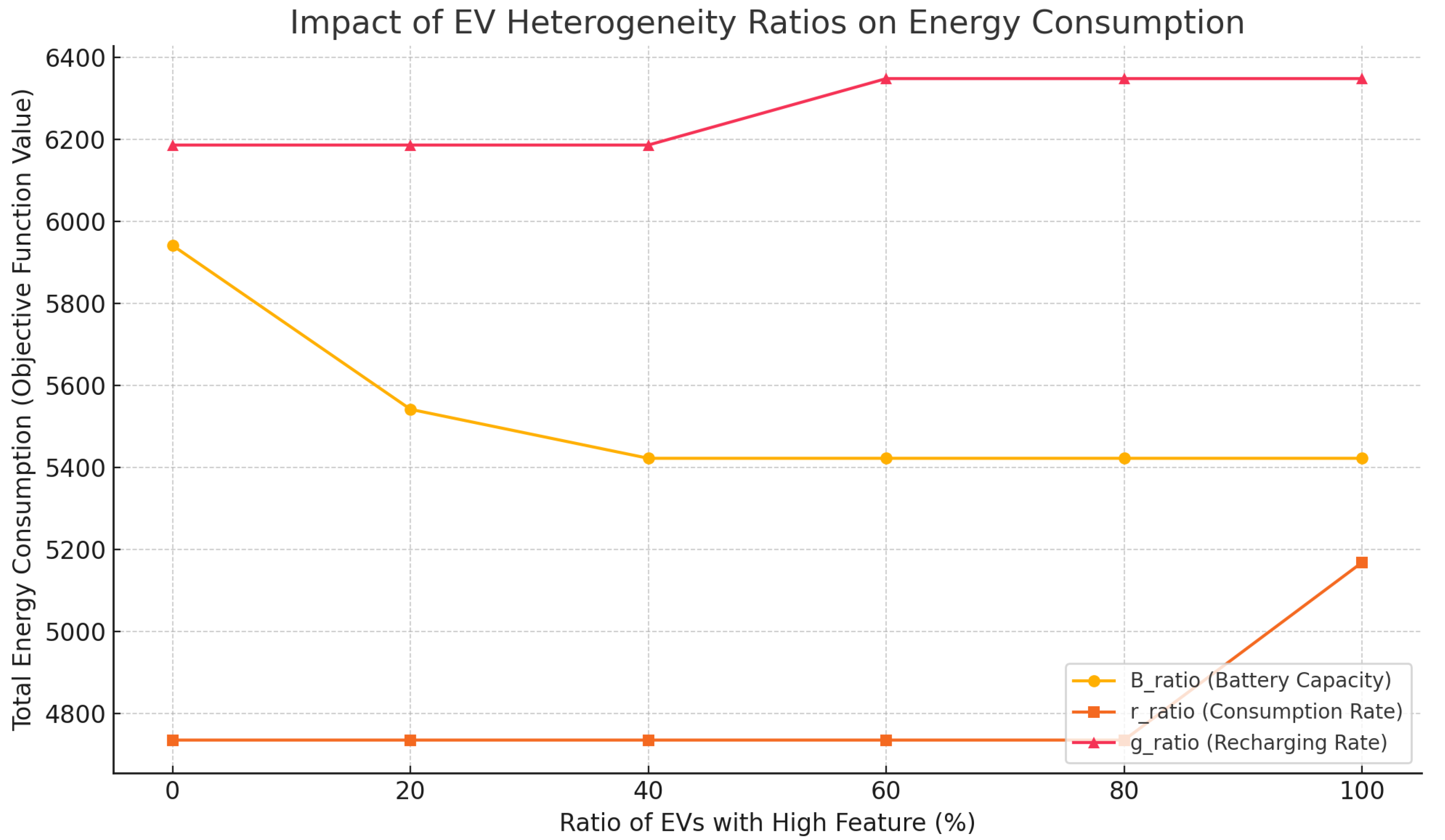
Figure 2.
Impact of the maximum number of active EVs on total energy consumption.
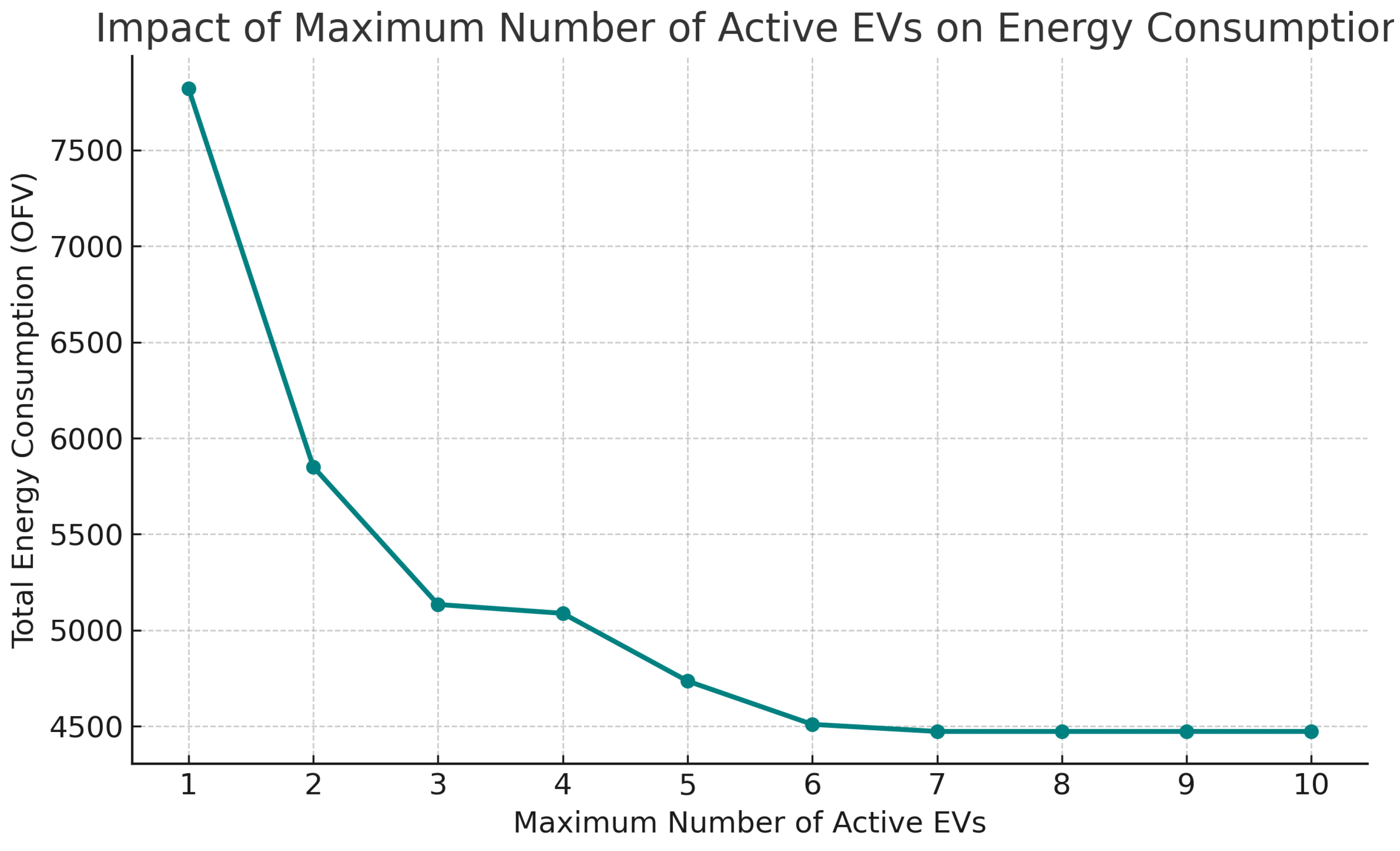
Figure 3.
Impact of payload-energy sensitivity coefficient () on energy consumption and number of used EVs.
Figure 3.
Impact of payload-energy sensitivity coefficient () on energy consumption and number of used EVs.
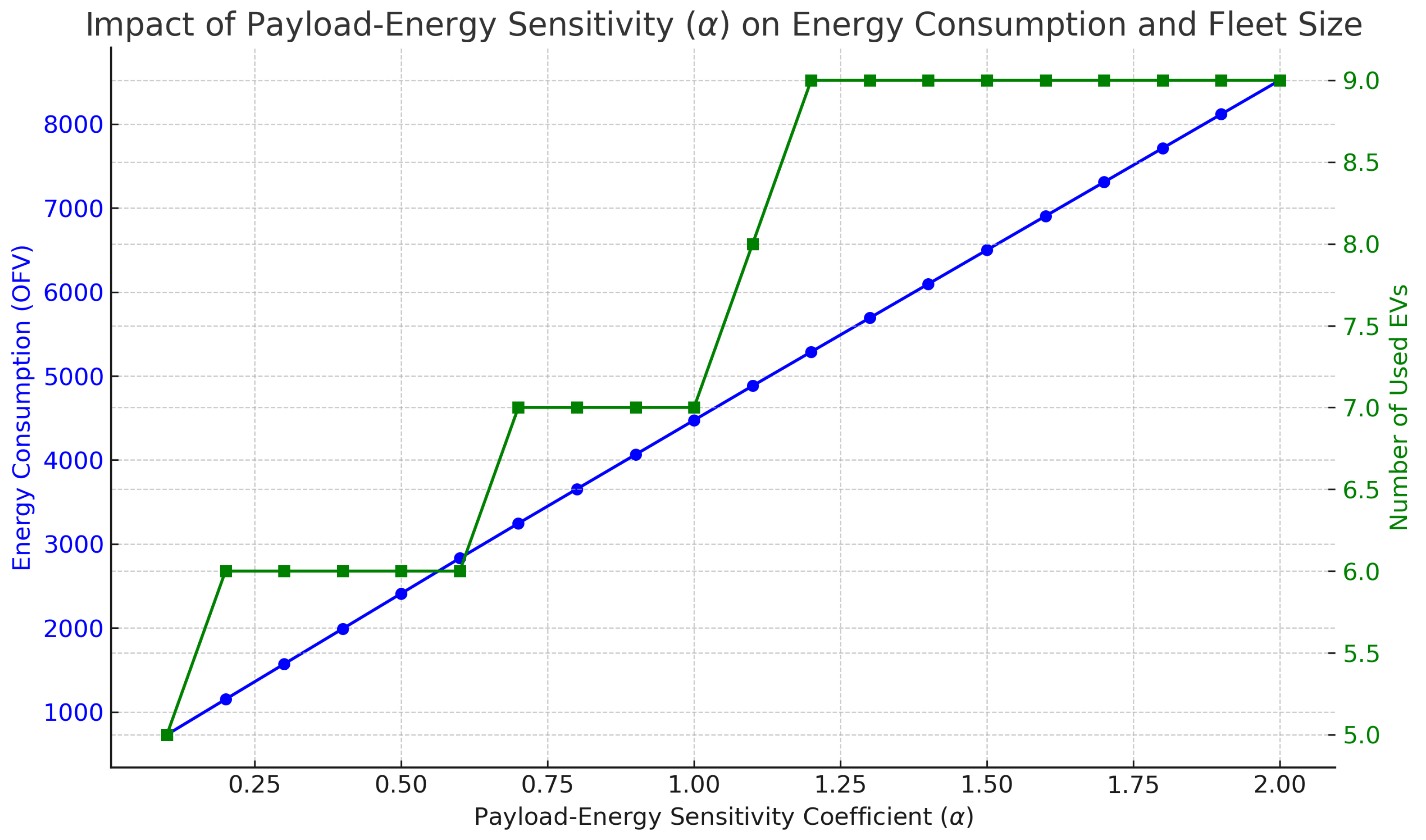

Table 1.
Comparison of HEVRP-TW studies in the literature.
| Reference | Problem Type | Methodology | Key Features |
|---|---|---|---|
| [6] | E-FSMVRPTW | MILP + VNS | Fleet size/mix, partial recharging, energy constraints |
| [7] | E-FSMVRPTW | MILP + ILS | Hybrid ILS, destroy-repair, recharging logic |
| [22] | HGVRP-TW with load-based energy model | Matheuristic | Mixed EV/ICE fleet, partial recharge, acceleration/deceleration effects |
| [21] | GMFVRP-PRTW | MILP + ILS | Partial recharge, mixed EV/ICE fleet, hard TW |
| [13] | HEVRP-TW with pickup-delivery | MILP + heuristic | SPD, recharging, heterogeneity |
| [23] | Bi-objective HGVRP-TW | MILP + GA + PBSA | Heterogeneous fleet, fuel limits, filling stations, time windows, emissions |
| [14] | EVRP with recycling | MILP + heuristic | Partial recharge, energy recycling |
| [15] | Bi-objective HEVRP-TW | MILP + NSGA-II | Mixed fleet, soft TW, cost-tardiness trade-off |
| [8] | HEVRP-TW with charger types | MILP + ALNS | Charger compatibility, soft TW, partial recharge |
| [8] | Multi-obj HEVRP-TW | MILP + -constraint + ALNS | Load-energy use, flexible recharge |
| [17] | SPD-HEVRP-TW | MILP + GA | Load-based energy, SPD, linear energy model |
| [18] | E-FSMVRPTW with partial recharge | Hybrid LS | Partial linear recharge, scalable search |
| [12] | HEVRP with soft TW | MILP + ALNS | Load-based energy, soft TW, heterogeneous fleet |
| [19] | HEVRP-TW | DRL | DRL + GAT, energy limits, deep learning policy |
| Present work | HEVRP-TW-EM | MILP | Mixed fleet, time windows, load-based energy consumption |
Table 2.
Notation and definition of decision variables and parameters.
| Sets: | |
|---|---|
| V | Set of all nodes, including depot, customers, and charging stations.; . |
| Set of intermediate nodes (excluding depot start/end); . | |
| Central depot. | |
| Dummy node representing the end depot. | |
| C | Set of customer nodes. |
| F | Set of charging station nodes. |
| K | Set of EVs. |
| A | Set of directed arcs, connecting the nodes; . |
| Parameters: | |
| Distance between node i and node j. | |
| Demand of customer i. | |
| Load capacity of vehicle k. | |
| Battery capacity of vehicle k. | |
| Battery consumption rate per unit distance for vehicle k. | |
| Battery recharging rate of vehicle k at charging stations. | |
| Upper bound on the number of used EVs. | |
| Travel time from node i to node j for EV k; | |
| Service time at node i. | |
| Earliest allowable arrival time (start of time window) at node i. | |
| Latest allowable arrival time (end of time window) at node i. | |
| A large constant used in time window constraints for linearization. | |
| Decision variables: | |
| Binary variable equal to 1 if vehicle k travels from node i to node j; 0 otherwise. | |
| Binary variable equal to 1 if vehicle k serves customer i; 0 otherwise. | |
| Load (payload) of vehicle k when traveling from node i to node j. | |
| Remaining battery level of vehicle k at node i. | |
| Arrival time of vehicle k at node i. |
Table 3.
Gurobi results for small-scale HEVRP-TW-EM instances with 5, 10, and 15 customers.
| Instance | Gurobi | Instance | Gurobi | ||||||
|---|---|---|---|---|---|---|---|---|---|
| OFV | Runtime | Opt. gap | OFV | Runtime | Opt. gap | ||||
| r104C5 | 5 | 2665.64 | 1.62 | 0.00 | c205C10 | 10 | 6357.73 | 48.30 | 0.00 |
| r105C5 | 5 | 2568.40 | 1.40 | 0.00 | rc102C10 | 10 | 6517.69 | 10.46 | 0.00 |
| r202C5 | 5 | 2001.62 | 2.30 | 0.00 | rc108C10 | 10 | 5298.83 | 35.30 | 0.00 |
| r203C5 | 5 | 3825.02 | 32.88 | 0.00 | rc201C10 | 10 | 5991.15 | 7200.00 | 1.27 |
| c101C5 | 5 | 6186.13 | 23.86 | 0.00 | rc205C10 | 10 | 6229.50 | 31.10 | 0.00 |
| c103C5 | 5 | 3229.54 | 2.06 | 0.00 | Average on C10 | 5662.28 | 737.04 | 0.11 | |
| c206C5 | 5 | 3344.86 | 6.26 | 0.00 | r102C15 | 15 | 5816.49 | 877.66 | 0.00 |
| c208C5 | 5 | 4911.11 | 1.68 | 0.00 | r105C15 | 15 | 6248.21 | 266.50 | 0.00 |
| rc105C5 | 5 | 7201.25 | 11.24 | 0.00 | r202C15 | 15 | 8237.51 | 7200.00 | 1.39 |
| rc108C5 | 5 | 6345.86 | 12.10 | 0.00 | r209C15 | 15 | 7066.05 | 287.30 | 0.00 |
| rc204C5 | 5 | 5610.40 | 3.64 | 0.00 | c103C15 | 15 | 9121.21 | 2667.52 | 0.00 |
| rc208C5 | 5 | 2607.91 | 1.90 | 0.00 | c106C15 | 15 | 5026.54 | 111.80 | 0.00 |
| Average on C5 | 4208.14 | 8.41 | 0.00 | c202C15 | 15 | 7948.18 | 241.32 | 0.00 | |
| r102C10 | 10 | 4735.70 | 27.12 | 0.00 | c208C15 | 15 | 8237.81 | 133.58 | 0.00 |
| r103C10 | 10 | 3074.45 | 35.53 | 0.00 | rc103C15 | 15 | 7254.19 | 281.52 | 0.00 |
| r201C10 | 10 | 4654.18 | 657.26 | 0.00 | rc108C15 | 15 | 10541.41 | 1004.88 | 0.00 |
| r203C10 | 10 | 3462.40 | 47.22 | 0.00 | rc202C15 | 15 | 8643.02 | 155.30 | 0.00 |
| c101C10 | 10 | 8630.36 | 661.04 | 0.00 | rc204C15 | 15 | 11112.61 | 143.08 | 0.00 |
| c104C10 | 10 | 5845.03 | 47.14 | 0.00 | Average on C15 | 7937.77 | 1114.21 | 0.12 | |
| c202C10 | 10 | 7150.31 | 44.04 | 0.00 | Average on all | 5936.06 | 619.89 | 0.07 | |
Table 4.
Gurobi results for medium-scale HEVRP-TW-EM instances with 30 customers.
| Instance | Gurobi | Instance | Gurobi | ||||
|---|---|---|---|---|---|---|---|
| OFV | Runtime | Opt. gap | OFV | Runtime | Opt. gap | ||
| c101_21 | 13333.20 | 7200.00 | 2.61 | r110_21 | 10857.39 | 7200.00 | 9.26 |
| c102_21 | 13191.43 | 7200.00 | 2.45 | r111_21 | 10830.94 | 7200.00 | 9.02 |
| c103_21 | 13170.00 | 7200.00 | 3.06 | r112_21 | 10756.79 | 7200.00 | 8.39 |
| c104_21 | 13028.54 | 7200.00 | 2.76 | r201_21 | 10960.45 | 7200.00 | 10.02 |
| c105_21 | 13359.29 | 7200.00 | 3.54 | r202_21 | 11075.42 | 7200.00 | 10.99 |
| c106_21 | 13318.12 | 7200.00 | 3.27 | r203_21 | 11868.99 | 7200.00 | 17.02 |
| c107_21 | 13381.94 | 7200.00 | 3.52 | r204_21 | 11133.02 | 7200.00 | 11.53 |
| c108_21 | 13216.90 | 7200.00 | 2.98 | r205_21 | 10741.26 | 7200.00 | 8.20 |
| c109_21 | 13159.66 | 7200.00 | 3.35 | r206_21 | 11611.42 | 7200.00 | 15.10 |
| c201_21 | 15392.41 | 7200.00 | 4.31 | r207_21 | 11346.90 | 7200.00 | 13.21 |
| c202_21 | 15210.10 | 7200.00 | 3.76 | r208_21 | 12535.59 | 7200.00 | 21.43 |
| c203_21 | 15012.60 | 7200.00 | 4.22 | r209_21 | 11074.93 | 7200.00 | 10.96 |
| c204_21 | 14964.33 | 7200.00 | 3.78 | r210_21 | 11361.24 | 7200.00 | 13.17 |
| c205_21 | 15940.81 | 7200.00 | 10.39 | r211_21 | 11230.89 | 7200.00 | 12.11 |
| c206_21 | 15007.82 | 7200.00 | 3.52 | rc101_21 | 26909.52 | 7200.00 | 7.10 |
| c207_21 | 15000.89 | 7200.00 | 3.87 | rc104_21 | 26469.49 | 7200.00 | 5.49 |
| c208_21 | 15089.60 | 7200.00 | 4.31 | rc105_21 | 26351.95 | 7200.00 | 5.03 |
| r101_21 | 11813.73 | 7200.00 | 12.37 | rc201_21 | 26515.20 | 7200.00 | 5.70 |
| r102_21 | 11073.65 | 7200.00 | 11.07 | rc203_21 | 26297.71 | 7200.00 | 4.99 |
| r103_21 | 10927.04 | 7200.00 | 9.84 | rc204_21 | 26702.59 | 7200.00 | 6.38 |
| r105_21 | 11519.83 | 7200.00 | 14.47 | rc205_21 | 29201.02 | 7200.00 | 14.43 |
| r107_21 | 14948.42 | 7200.00 | 34.08 | rc206_21 | 25934.07 | 7200.00 | 3.61 |
| r108_21 | 10672.22 | 7200.00 | 7.75 | rc207_21 | 28643.59 | 7200.00 | 12.73 |
| r109_21 | 10857.39 | 7200.00 | 9.26 | rc208_21 | 27149.98 | 7200.00 | 7.92 |
| Average | 15628.13 | 7200.00 | 8.51 | ||||
Table 5.
Gurobi results for medium-scale HEVRP-TW-EM instances with 40 customers.
| Instance | OFV | Runtime Gurobi |
Opt. gap |
|---|---|---|---|
| c101_21 | 21402.07 | 7200.00 | 5.94 |
| c103_21 | 31510.52 | 7200.00 | 36.45 |
| c105_21 | 22054.28 | 7200.00 | 8.95 |
| c106_21 | 22623.28 | 7200.00 | 11.30 |
| c107_21 | 21401.59 | 7200.00 | 6.22 |
| c109_21 | 24618.05 | 7200.00 | 11.06 |
| c203_21 | 25215.38 | 7200.00 | 13.45 |
| c205_21 | 25191.36 | 7200.00 | 13.29 |
| c207_21 | 25320.48 | 7200.00 | 13.71 |
| r101_21 | 15944.53 | 7200.00 | 9.06 |
| r105_21 | 15828.43 | 7200.00 | 8.39 |
| r109_21 | 15826.32 | 7200.00 | 8.38 |
| r110_21 | 15879.98 | 7200.00 | 8.60 |
| r111_21 | 16049.00 | 7200.00 | 9.60 |
| r112_21 | 15789.88 | 7200.00 | 8.12 |
| r201_21 | 15795.28 | 7200.00 | 8.19 |
| r203_21 | 21750.38 | 7200.00 | 33.34 |
| r205_21 | 15705.50 | 7200.00 | 7.67 |
| r209_21 | 15955.82 | 7200.00 | 9.06 |
| r210_21 | 15903.13 | 7200.00 | 8.83 |
| r211_21 | 15699.03 | 7200.00 | 7.65 |
| Average | 19784.01 | 7200.00 | 11.77 |
Disclaimer/Publisher’s Note: The statements, opinions and data contained in all publications are solely those of the individual author(s) and contributor(s) and not of MDPI and/or the editor(s). MDPI and/or the editor(s) disclaim responsibility for any injury to people or property resulting from any ideas, methods, instructions or products referred to in the content. |
© 2025 by the authors. Licensee MDPI, Basel, Switzerland. This article is an open access article distributed under the terms and conditions of the Creative Commons Attribution (CC BY) license (http://creativecommons.org/licenses/by/4.0/).
Copyright: This open access article is published under a Creative Commons CC BY 4.0 license, which permit the free download, distribution, and reuse, provided that the author and preprint are cited in any reuse.


