
Submitted:
05 February 2025
Posted:
06 February 2025
You are already at the latest version
Abstract
The current environmental challenges demand immediate actions, especially in the transport sector, one of the largest CO2 emitters. Vehicle electrification is considered an essential strategy for emission mitigation and combating global warming. This study presents methodologies for modeling and energy management of microgrids (MG), designed as charging stations for electric vehicles (EVs). Algorithms were developed to estimate daily energy generation and charging events in the MG. These data feed an energy management algorithm aimed at minimizing the costs associated with energy trading operations as well as the charging and discharging cycles of the battery energy storage system (BESS). The problem constraints ensure the safe operation of the system, availability of backup energy for off-grid conditions, preference for reduced tariffs, and optimized management of BESS charge and discharge rates, considering battery wear. The grid-connected MG used in the case study consists of a wind turbine (WT), photovoltaic system (PVS), battery energy storage system (BESS), and an electric vehicle fast-charging station (EVFCS). Located on a highway, the MG was designed to provide fast charging, extending the range of EVs and reducing drivers’ range anxiety. The study results demonstrated the effectiveness of the proposed energy management approach, with the optimization algorithm efficiently managing energy flows within the MG while prioritizing lower operational costs. The inclusion of the battery wear model makes the optimizer more selective in battery usage, operating it in cycles that minimize BESS wear and effectively prolong its lifespan.
Keywords:
EV Microgrid
; Highway EV fast-charging
; Energy Dispatch in MG
; Energy Management Optimization
; Energetic Transition
; Operational Cost Minimization
1. Introduction
The global imperative to mitigate greenhouse gas emissions has intensified efforts toward sustainable energy transitions, with the transportation sector playing a key role. According to the International Energy Agency (IEA), energy-related emissions reached a record high of 37.4 billion tonnes in 2023, underscoring the urgent need for decarbonization strategies [1]. The transportation sector consumes over 30% of global energy and significantly contributes to emissions, accounting for nearly 20% of the total. Among the various modes of transport, road transport remains the predominant source of greenhouse gas emissions within this sector [2].
Electric vehicles (EVs) have emerged as a cornerstone of this transition, accelerating worldwide adoption. In Brazil, the EV market, though currently representing a modest share of total automobile sales, has exhibited significant growth. Projections indicate that the Brazilian electric vehicle market is expected to grow by 17.1% on an annual basis, reaching USD 1.2 billion by the end of 2024 [3]. The IEA projects that by 2035 the number of EVs in the world will reach the mark of 525 million vehicles, where one in 4 vehicles will be electric [4].
The expansion of the EV fleet necessitates a corresponding development in charging infrastructure, particularly along highways to support long-distance travel. The integration of distributed energy resources (DERs) into these charging stations presents an opportunity to enhance sustainability but also introduces challenges such as managing intermittent generation and preventing reverse power flow during peak production periods [5].
Effective Energy Management Systems (EMS) are essential to address these challenges, optimizing the interaction between distributed generation (DG), Battery energy storage systems (BESS), and the grid. A critical aspect of EMS optimization involves accounting for storage degradation, which impacts both the economic and operational efficiency of EV fast-charging stations (EVFCS).
This study proposes an optimized EMS strategy for EV fast-charging microgrids incorporating storage degradation considerations. By leveraging predictive algorithms and real-time data, the proposed system aims to enhance energy efficiency, reduce operational costs, and extend the lifespan of storage components, thereby contributing to the sustainable expansion of EV infrastructure in Brazil and beyond.
1.1. Highlights of this Paper
Some contributions of the paper are cited as follows:
- Integration of load, generation, and storage elements, including EVFCS, BESS, PV, and WT, in the proposed microgrid (MG) framework.
- Utilization of Time-of-Use (ToU) tariffs and allow exploration of additional pricing mechanisms, such as Day-Ahead Market tariffs, for cost optimization.
- An objective function focused on minimizing MG operational costs by prioritizing BESS usage and self-consumption of locally generated energy.
- Inclusion of BESS degradation in the optimization problem to ensure realistic and sustainable storage management.
- A flexible and modular design, allows scalability to larger problems and the incorporation of additional components within the MG.
- Modeling approach based on Python, leveraging free algorithms, packages, and solvers to promote accessibility and replicability.
- Renewable generation estimation based on meteorological forecasts combined with physical models, improving prediction accuracy.
- Load consumption estimation leveraging historical data from EVFCS operations, enabling more accurate forecasts as usage patterns evolve.
- Modular models for generation, charging, and EMS algorithms, allowing seamless updates and replacements with improved versions.
1.2. Delimitations of Paper
Although the paper proposes highly flexible methodologies that can be adapted to other scenarios and studies, it is important to highlight some limitations:
- The model is developed for highway scenarios, where the dynamics of FCS focus on avoiding queue formation, prioritizing quick charging sessions without considering extended parking times or energy exchanges via vehicle-to-grid (V2G).
- Future applications may partially leverage the methodologies developed here for urban parking or rural contexts, adjusting them to meet the specific needs of these scenarios.
- The primary focus of the paper is on EMS, with other topics related to MG operation falling outside the scope of this study.
2. Literature: Analysis and Contextualization
The incorporation of renewable energy resources has led to a significant rise in the deployment of DER within energy systems. These DERs, when combined with associated loads, constitute an MG [6]. As defined by the National Renewable Energy Laboratory (NREL), a MG is a system comprising interconnected loads and DERs that function as a unified controllable entity relative to the main power grid. This system can operate in two distinct modes: grid-connected, where it interfaces with the main grid, or islanded, where it functions independently [7].
Considering the increasing adoption of MGs, the development of usage and management strategies has become a critical requirement for these systems. In the literature, optimization problems are commonly addressed with objectives such as minimizing costs, energy losses, or recharge times, as well as maximizing profits, energy sales, efficiency, renewable energy utilization, and other performance metrics [6].
Reference [8] proposes a method of MG management to maximize discharge/charge rates, based on tariff preferences. The generation of DERs is based on typical profiles. While in [9] a new battery wear model is based on a V2G application model, adapted for use in MGs. It calculates wear costs based on changes in the state of charge (SoC) during discharge/charge events. WT is not incorporated in this work.
Authors in [10] bring new scheduling methodology that considers the Depth of Discharge (DoD) and SoC levels to minimize battery degradation, achieving a reduction in the capacity loss by more than 30% in simulations. The applications of this study involve V2G transactions, which do not apply to road contexts.
The study [11] develops a planning strategy for EV charging stations to maximize operator profits, considering investment costs, revenue, and variable costs, using an algorithm that iteratively adds stations to meet charging needs while optimizing facility utilization. The system proposed by [12] is designed for MGs operating in isolated areas, utilizing a Renewable-Based Energy Management System (RBEMS) that analyzes historical data and short-term forecasts to determine setpoints for renewable generation and programmable loads in a cost-effective, reliable, and sustainable manner.
On the other hand, some studies are focused on the residential context, as in the study [13] explores energy management options for EV charging stations in buildings, with a focus on increasing power grid capacity without increasing peak demand. It emphasizes adaptable solutions to seasonal and daily demand variations, promoting sustainable transport ecosystems in urban areas.
Some literature works with energy management, considering charging stations in cities. The paper [14] features a cost-effective energy management system for fast charging stations by integrating solar PV and energy storage systems. It focuses on optimizing the charging of electric vehicles in urban environments, increasing sustainability, and reducing reliance on fossil fuels. In addition to not considering WT, the implementation of EMS is done via commercial software, which can bring additional costs to the operator. Many studies do not consider the allocation of BESS, while others only look at the integration of fast-charging EVs with PVS plants [15].
Classical programming methods are quite common in the literature for modeling and operation of EMS, as is the case of [16] which discusses the optimal planning and dispatch of BESS in MGs, with a focus on improving cycle life through a mathematical model formulated as a Mixed Integer Linear Programming (MILP) problem and solved using GUROBI. The study was validated in a test MG. Like other papers presented, the dependence on commercial solvers can lead to unforeseen expenses.
EMS for EVFCS along highways are essential to optimizing operational efficiency, reliability, and sustainability of charging infrastructure. These systems leverage advanced control strategies to address critical challenges such as peak demand mitigation, cost minimization, and grid stability enhancement. Core functionalities include real-time load balancing to prevent grid overloading, integration of DER to reduce emissions, and the utilization of Energy Storage System (ESS) to buffer demand fluctuations. Predictive algorithms and demand forecasting are employed to optimize energy allocation, minimizing charging times and enhancing user satisfaction. Through these integrated strategies, EMS for EVFCS facilitates the scalable and sustainable expansion of electrified highway systems [17,18].
Other approaches consider the energy management for the island group energy system, as in [19].The article introduces a Hybrid Policy-based Reinforcement Learning (HPRL) approach for adaptive energy management in energy transmission-constrained island groups. It proposes an Insular Energy Hub (IEH) model that enables cascading energy utilization, addressing the specific energy demands of islands while ensuring supply reliability. Furthermore, the Energy Management Model for Island Groups (EMIG) is formulated to account for the inverse distribution of demand and energy resources, transforming the challenge into a model-free reinforcement learning task. The effectiveness of the approach was demonstrated through numerical simulations. For now, the focus of the optimization in this paper is on the grid-connected operation with a single MG. Future research may address energy management considering more MGs and their cooperation to meet the goals at reduced costs.
Taking into account the findings and possible deficiencies found in the literature, this study proposes a programmed management of MG. Here, DER generation models are updated daily, based on the predicted weather data, and obtained via reliable Application Programming Interface (APIs) [20]. This provides better assertiveness since the generation of plants is correlated with meteorological data [21]. Weather models have evolved significantly and are now widely used for accurate weather and weather-related forecasts. In addition, the integration of a BESS contributes to increasing the reliability of the MG and ensuring that there is operation even off-grid. The consideration and implementation of a BESS wear model contribute to a more balanced use of the system, avoiding overuse and premature end-of-life.
The inclusion of hourly tariffs enables the EMS to make informed decisions aimed at reducing energy costs by purchasing electricity during lower-cost periods. The modularity of the EMS algorithm’s input data facilitates continuous calibration and improvement of each submodel that constitutes the overall model. The proposed EMS also accommodates updates to net metering value discounts for sold energy. Furthermore, two options are presented to estimate charging demand in the EVFCS. The first option provides estimations for initial operations, where the station’s usage patterns are yet unknown. The second option allows for updates based on an established database, enabling the estimation of the EVFCS load curve by analyzing trends observed in historical data.
3. Proposed Methodology
The proposed methodology for MG management integrates meteorological data and mathematical models to predict the energy generated from renewable sources throughout the day. In addition, the values of the electricity tariff and the EV recharging events estimated for the day of operation are considered. Based on this estimated information, the dispatch of the BESS is programmed by the energy management algorithm. The dispatch profile resulting from this optimization is sent via the internet to MG’s central industrial computer, which passes the defined set points to the Programmable Logic Controller (PLC), which controls BESS dispatches throughout the day. Figure 1 presents a schematic summary of the complete methodology.
The following shows the modeling carried out to estimate the recharges in the MG, the generations coming from WT and PVS, the BESS wear model is detailed, and later the algorithm developed to optimize the energy management in the MG is presented.
3.1. EVFCS Usage Modeling
Forecasting and analyzing the demand for EV charging on highways faces significant challenges, as they rely on several external and unpredictable factors, such as mobility patterns, seasonality, weather, and human behavior. To address these uncertainties, several models have been developed, including approaches based on statistical data, learning from historical usage patterns, traffic surveys, and vehicle flow counts, among others.
In [22], a methodology is presented to model typical vehicle usage profiles in Brazil, categorized according to the types of trips undertaken, enabling the estimation of charging demand. In turn, the study in [23] builds upon these typical usage profiles for regular users and complements the analysis by including occasional users, modeled through simulations based on the Monte Carlo method. However, both approaches are focused on charging in residential contexts and parking lots, without considering the specificities of charging behavior on highways, which require a different analysis due to their unique characteristics and greater variability.
In the context of highways, two possible alternatives can be highlighted. The first is intended for initial operations, where a consolidated history of recharging data is not yet available. The second leverages observed patterns in the recharging behavior, such as energy consumption, recharge duration, and connection time. Therefore, at first, it is possible to use the methodology developed in [24], since there is no history of recharges. The daily capacity behavior of the establishment, the typical variation of flow on the highway, the market share of EVs and the distribution of battery capacities of the EVs sold, served as a basis for estimating recharging events and then the EVFCS usage pattern [24].
As a second option, already knowing the user’s behavior, the EVFCS demand curve will be obtained from the statistics of the recharge history. This is a more attractive option and will be used in this work. The algorithm developed follows the following step-by-step, which are illustrated in Figure 2:
- Load and Clear Data: Organize historical data.
- Filter Relevant Data: Eliminate database errors, erroneous data, and outliers.
- Analyze Trends: Identify historical patterns.
- Generate Usage Profile: Create probabilistic models.
- Simulate Scenarios: Generate daily recharge distributions based on historical patterns.
- Preview Results: Show the simulated and average curves.
- Export Data: Save results for integration with other systems.
Figure 3 shows a daily recharge profile obtained following the process described above. This profile was generated from historical recharge data, which was organized, filtered, and analyzed to identify patterns of behavior. Subsequently, probabilistic modeling was used to create representative distributions of the characteristics of the recharges, such as duration, energy consumed, and start times. Based on these distributions, daily scenarios were simulated that reflect the typical use of the EVFCS. Finally, the results were viewed and exported for integration into the EMS algorithm.
3.2. Wind Generation Modeling
The use of wind kinetics for the generation of electricity depends on factors such as wind speed, turbine sweep area, characteristics of the installation site, such as soil roughness, altitude, and the construction characteristics of WT [25,26,27].
There are different types of models used for wind generation forecasting. The main methods include physical, statistical, and hybrid models. The physical models are based on principles of fluid mechanics and the technical characteristics of the turbines, such as the power curve and the geometry of the blades, and are fed by meteorological data, such as wind speed and direction, obtained by numerical forecasts or local measurements [28,29].
Statistical models, on the other hand, use methods such as linear regression and time series to identify historical patterns, offering quick solutions, but with limitations in scenarios of high variability. Hybrid models combine physical and statistical approaches, integrating machine learning techniques to capture complex relationships between the variables involved [28,29]. The choice of model depends on the requirements of accuracy, time horizon, and data availability, with physical models standing out for their robustness when fed by detailed weather forecasts.
Deterministically, it is possible to calculate the mechanical power available in a wind turbine using eq. (1):
where is the mechanical power of the turbine (W, kW, or MW), is the air density (kg/m3), is the power coefficient of the turbine or Betz limit, A is the rotor area (m2), and is the wind velocity approaching the turbine (m/s). The air density is approximately 1.225 kg/m3 under standard conditions of temperature and pressure (1 atm, 15.56 °C, at sea level). References [25,30] highlight that it is possible to estimate the air density based on the altitude of the location, when necessary. The higher the altitude, the more rarefied the air becomes, leading to a lower density [25,30].
Consequently, the electrical power generated by a WT is given by eq. (2);
where is the electrical power delivered (W, kW, or MW), and is the total efficiency of the wind turbine system, including components such as the generator, gearbox, mechanical losses, and electrical losses [25].
It is also possible to calculate the power generated by the wind turbine, through the turbine power curve provided by the manufacturer from tests. This curve relates the output power generated to the wind speed incident on the turbine blades. Figure 4 shows a power curve as a function of wind speed for the 30 kVA WT.
Wind power generation is only possible above a minimum wind speed (cut-in speed) and varies with wind speed and turbine characteristics until reaching the cut-out speed, at which point the turbine must be shut down. Wind speed at the turbine blades must be adjusted, as API data typically provides wind speeds measured at 10 meters above ground. The Hellman Law is widely used in engineering and meteorology to extrapolate wind speeds from a reference height to a height z, considering the terrain properties and the logarithmic wind profile. This law provides a practical way to estimate wind speeds at different heights based on terrain roughness [27,31]. The basic formula of the Hellman Law is expressed as eq. (3).
In this eq. (3), represents the wind speed at height z (in m/s), while is the wind speed at the reference height (in m/s). The variable z denotes the height at which the wind speed is to be extrapolated (in meters), and is the reference height where the wind speed is already known (in meters). The exponent depends on the roughness of the terrain and is an empirical parameter that varies with the type of terrain and atmospheric conditions.
The value of typically varies depending on the roughness of the terrain. For example, for water surfaces or very flat terrains, . In rural areas or regions with low vegetation, . In suburban areas or regions with medium-sized constructions, . Finally, for urban areas or regions with tall buildings, . The Hellman Law is a practical tool for estimating wind speeds at various heights. However, its accuracy depends on the assumption of a constant wind profile and the consistency of terrain roughness. Abrupt changes in terrain or atmospheric instability can reduce the precision of this method.
Via weather API, wind speed forecasts are obtained for the next day. Data interpolation manipulations are performed every 5 minutes, and the wind speed is corrected, via Hellman’s Law, for the height of the wind turbine. Thus, it is possible to calculate the generation, as shown in the diagram in Figure 5.
3.3. PV Generation Modeling
Photovoltaic generation forecasting methods are widely used to optimize the use of solar energy, and are divided into three main approaches: based on physical models, statistical methods, and artificial intelligence techniques. Physical models use meteorological information and characteristics of photovoltaic systems, such as solar radiation and ambient temperature, to estimate energy generation based on physical principles. Statistical methods, on the other hand, apply time series and mathematical models, such as linear regression and ARIMA, to identify historical patterns and make short-term predictions [32,33,34].
On the other hand, artificial intelligence techniques such as Artificial Neural Networks (ANN), machine learning, and hybrid algorithms offer more accurate forecasts by learning from large volumes of historical and weather data. The combination of physical models from the panels with weather forecast data has significant advantages, such as greater accuracy when incorporating real-time weather conditions or day-ahead forecasts and adaptability to local variations, allowing you to optimize energy generation and planning more efficiently and reliably [32,33,34].
The calculation of photovoltaic generation is based on the nominal power of the module, the rate of reduction of the efficiency of the photovoltaic module due to degradation, solar irradiation at the installation site, and the temperature of the module, according to the eq. (4) [33,35].
where is the output power of the photovoltaic module (kW) at hour h, is the nominal power of the photovoltaic module under standard test conditions (kW), is the efficiency reduction factor of the photovoltaic module due to degradation (%), is the total irradiance on the surface of the Earth (W/m2) at hour h, is the irradiance under standard test conditions, assumed to be 1000 W/m2, is the power temperature coefficient (%/°C), is the photovoltaic panel temperature (°C) at hour h, and is the photovoltaic panel temperature under standard test conditions, assumed to be 25°C [33]. All parameters under Standard Test Conditions (STC) correspond to those tested by manufacturers in laboratory conditions.
The modeling of the cell temperature in the photovoltaic panel is directly related to ambient temperature and solar irradiance. Equation (5) presents this approach, where is the ambient temperature measured at hour h, is the hourly irradiance, and Nominal Operating Cell Temperature (NOCT) is the nominal operating cell temperature of the photovoltaic panel [36,37].
Finally, the output power per photovoltaic panel was estimated using eq. (4), the total power generated is proportional to the power of each panel and the number of panels installed, , as shown in eq. (6). It is worth mentioning that the photovoltaic generation model considers panels with the same generation capacity, positioned similarly, and under similar conditions, accounting for shading and surface states.
This mathematical approach aligns with the methodology employed by the Homer software to calculate a plant’s photovoltaic generation. can be inserted into the software as a text file with hourly data, generated from Typical Meteorological Year (TMY) data for the location. In the absence of such data, Homer uses the Graham algorithm to generate synthetic irradiance series [38]. This algorithm produces hourly irradiance values based on latitude and monthly average irradiance values. Therefore, it allows energy estimates for long periods.
However, for the short term, the data obtained via weather API for the next day ensures better accuracy and precision in estimating the photovoltaic generation profile. The sequence of steps followed is shown in Figure 6. Since the data comes in every hour, some manipulations and interpolations are required to obtain a daily profile with 5-minute discretization, which will be the resolution used in the optimization algorithm.
3.4. BESS Degradation Cost Model
BESS is costly, especially considering their limited lifespan, as batteries can only endure a finite number of charge-discharge cycles before reaching the end of life (EOL), typically defined as a 20%–30% reduction in the state of health (SoH) [39]. The degradation of li-ion batteries occurs as a function of variables such as temperature, calendar effect, intensity of discharges, and applied currents, among other factors, according to [40,41,42,43]. Among the available technologies, lithium-ion batteries (LIBs) and lead-acids are predominant in modern BESS applications.
Various models are used in the literature to predict and mitigate battery degradation. Empirical and semi-empirical models are widely used due to their simplicity and ability to provide quick estimates based on experimental data. These models correlate the number of charge/discharge cycles with the depth of discharge and temperature. This work uses the modeling presented by [9], which updates the empirical battery wear model proposed by [44] considering the battery’s wear as a function of the intensity of discharge. So, the total cycles of a battery are reduced when it is subjected to high DoD.
In the literature, some functions are proposed to relate the Achievable Cycle Count (ACC) to the DoD. Since life cycle data is often presented at discrete DoD levels, interpolation is useful. To achieve this, a generic function can be defined in various formats to fit different wear curves. In [44] is proposed the reciprocal function , where and are curve-fitting coefficients, but it has limitations in universality. Alternative formats, such as the exponential, and logarithmic, , also fit specific cases well but fail to generalize. To address this, a combined reciprocal and exponential model is proposed by [9] for broader applicability, as shown eq. (7).
where , and are coefficients that can be obtained by methods such as the least squares fitting, and d is the DoD of BESS. Considering the cost, capacity, and ACC vs DoD curve of the BESS, and performing the necessary mathematical manipulations, [9] derived a Normalized Wear Density Function, , expressed in terms of monetary cost per unit of energy transferred (typically $/kWh), as shown in eq. (8). This formula allows you to calculate the density of wear as the DoD varies.
where is a modulating factor to account for temperature fluctuation, calculated as , where is the temperature of the battery in Celsius. The is the BESS price ($), M represents the BESS capacity (kWh), and is the current DoD of the BESS.
The average value of the Wear Density Function is useful for assessing the cost-benefit of different battery models, as it considers not only price and capacity but also durability. The average value of eq. (8) is calculated as eq. (9):
Since has nonlinear variation behavior as a function of the SoC, it is necessary to use a piecewise linearization algorithm to insert this variable into linear optimization problems [45].
3.5. Proposed Optimization Algorithm
The main objective is an optimized power distribution between the grid and BESS according to the utilization of local renewable energy production and the reduction of operating costs. Therefore, the controllable power rate defines when the BESS charges or discharges energy. These are the decision variables for the optimization problem. This formulation was chosen for its maturity, availability of tools, and fast and robust convergence to the global optimum.
A formal description of this optimization requires definition of the following parameters and variables, as summarized in Table 1.
The MG energy management problem involves the optimization of static storage discharge/charge events to meet the charging demands of EVs while reducing operating costs. In this sense, charging is preferred when it is cost-effective, or discharging is preferred when energy costs are high, given the variation in hourly electricity price. The dispatch scheduling problem is approached by time window, so that the total available period for discharging/charging during the day is uniformly distributed over a sample interval within intervals, as in eq. (10).
Note that the problem only comprises unidirectional charging of EVs and bidirectional discharging/charging of BESS. Thus, the EMS should preferentially dispatch power from the BESS during periods of peak tariff, while prioritizing dispatch from the grid when the tariff is cheaper. It is important to emphasize that the energy coming from PVS and a WT is constantly used by the MG in the form of constraint. It is more efficient to use the generated energy directly for charging EVs, without losses from conversion to BESS. When there is no charging of EVs, the energy is injected into the grid by the net metering system or it is stored in the BESS.
The objective function (OF) consists of scheduling the discharging/charging of the BESS to minimize the costs of buying, selling, and storing energy, according to eq. (11). The optimal power dispatch between local renewable sources, BESS, or grid is determined at each time instant j to achieve the objective and ensure the correct MG operation. When energy is sold to the grid, the cost considered is the loss in the value of the kilowatt-hour by the net metering discount.
The constraints of the optimization problem comprise (a) energy balance, (b) SoC of the BESS, and (c) BESS power. An energy balance constraint is set to ensure that the load on the MG is equivalent to the energy consumed, according to eq. (12).
The loads are the total power required to charge the connected EVs () and the power to charge the BESS (). Also, there is power injected into the grid (). As the energy source, we have a photovoltaic generation (), wind generation () and the BESS discharging power (). Also, there is the amount of energy purchased from the grid ().
Full participation of photovoltaic and wind generation in the form of an energy balance constraint is assumed. In this way, the conversion of energy to the battery is prevented by using it at the same instant of generation and EV connection, bypassing possible efficiency losses. In the case of highway fast charging, the demand for EVs is not controllable, so, like local renewable generation, it cannot be visualized in the objective function, but it is present in this energy balance constraint.
Note that power available by photovoltaic () and wind () systems are the estimated at each time instant, j. As already described, wind and photovoltaic daily generation profiles are obtained from physical models, fed with wind and irradiance data obtained via weather forecast APIs [20].
The maximum power requested and supplied to the grid () are constrained as a tool to prevent overload of the distribution transformer for any time instant j. This restriction can be fixed or variable in time to limit energy purchases in periods of higher tariffs, depending on the tariff structure addressed. In this case, a fixed value is considered, since the ToU adopted for the case study bills only the amount of energy and not the power. Furthermore, a binary power exchange logic is formulated to prohibit the scenario of energy purchase and injection at the same instant of time j, according to eq. (13) and eq. (14).
where is a binary auxiliary parameter used to indicate whether energy should be purchased or injected into the grid, according to eq. (15).
The BESS can be charged, discharged, or remain inactive at each time step. Thus, BESS scheduling is decomposed into two variables, one for charging () and one for discharging (), for . Both discharging/charging powers are controllable and constrained by their upper limits, i.e., ( and ), respectively, according to eq. (16) and eq. (17). The power exchange logic is implemented to make it impossible to charge and discharge simultaneously, according to eq. (18).
where, is a binary auxiliary parameter used to indicate when the BESS is charged or discharged, according to eq. (18).
At the beginning of each day, the initial BESS SoC is computed, according to eq. (19).
As a guarantee that there will always be an amount of power remaining in the BESS, to keep the operation offline, and provide emergency recharges, in the problem the initial SoC, , is set at least 50%. Likewise, at the end of the simulation day, the final SoC is required to be at least equal to 50%, i.e., .
According to eq. (20) always at the beginning of the day, the BESS SoC should be equal to or greater than the initial one, . Thus, 288 is the total j period in a day, and is the total days in the chosen period (7 in a week, 30 in a month, and 365 in a year). Obviously, for simulations of only one day, this restriction can be disregarded or set a value of 1 for .
The current SoC () at any time instant j, denoted by eq. (21), can be obtained by considering:
- The SoC at the previous time step ();
- The increment of SoC as a result of charging;
- The SoC decrease due to discharging.
As the BESS serves as a power source in the MG, there must be a minimum amount of energy to provide power to EVs. To guarantee such a minimum requirement for the next day, BESS’s SoC must satisfy a minimum threshold at the last time step of the current day’s scheduling, according to eq. (23).
Another restriction that can be used refers to the maximum total charge and discharge cycles that the BESS can have during the total period considered. In this way it is possible to reduce the loss of capacity of the BESS due to the wear of the system by the excess of cycles, as equated in eq. (24) and eq. (25).
where is the maximum total number of charging cycles.
where is the maximum total number of discharge cycles. These parameters can be useful if considering periods longer than 1 day of simulation. Thus, the operation of the BESS can be limited to a maximum number of charge and discharge cycles, defined by the owner of the MG.
To ensure efficient operation and preserve the life of the BESS, restrictions have been imposed that prevent abrupt changes between the loading and discharging states. These restrictions ensure that the BESS goes through a transition state, called idling, in which it performs neither loading nor unloading before switching between these two modes of operation.
The first constraint prevents the BESS from switching directly from the discharging mode to the charging mode. In this case, if the system was discharging in the previous period (), it cannot enter charging mode in the current period (), ensuring that the charging state is zero (). The constraint can be mathematically expressed in eq. (26).
Similarly, the second constraint prevents the BESS from switching directly from charging mode to discharging mode. Thus, if the system was charging in the previous period (), it cannot enter discharging mode in the current period (), ensuring that the discharging state is zero (). This relationship is mathematically represented in eq. (27).
These restrictions ensure that BESS operates in a stable manner, avoiding behavior that could cause premature wear and damage to the system. In addition, this approach promotes a more controlled transition between operating modes, contributing to the reliability and efficiency of the system.
In addition to technical and operational constraints, other constraints may also be included in the model. Some restrictions defined by the authors are presented below to better personalize the study.
Restriction 1: The restriction ensures that the BESS will be charged only when there are no recharges in progress in the system. The inequality of eq. (28). limits the surplus of DER used to charge the BESS, ensuring that this process occurs only in the absence of other recharges. This restriction prevents excessive energy demand from the grid at the same time.
Restriction 2: The restriction imposes a limit on the charge of the energy storage battery (BESS), ensuring that it does not exceed the instantaneous sum of the power generation of the wind and photovoltaic at the instant j. This condition is necessary to ensure that BESS charging only uses the energy available from the DER, avoiding the use of external sources or the violation of the physical limits of the system, as eq. (29).
Restriction 3: The restriction states that the discharge power of the BESS may not exceed the maximum charging power requested by electric vehicles at the instant j. This limitation ensures that the BESS discharges only the energy necessary to meet instantaneous demand, avoiding overloading or wasting energy, while keeping the system compliant with operational requirements, as shown eq. (30).
Restriction 4: The restriction limits the maximum power that can be injected into the electricity grid, ensuring that this power does not exceed the sum of distributed generation from wind and photovoltaic sources at the instant j. This formulation allows for dynamically controlling the power injection into the grid, ensuring that the injection is limited or allowed according to the availability of distributed generation, as shown eq. (31).
Restriction 5: The restriction ensures that at least 80% of the energy generated by DERs (wind and photovoltaic) is consumed locally, limiting the injection of energy into the electricity grid to a maximum of 20% of the total generated, as shown eq. (32).
This restriction promotes the efficient use of locally generated energy, reducing dependence on the power grid and minimizing losses related to transmission and distribution. In addition, it is aligned with sustainable practices and incentives for the self-consumption of renewable energy.
4. Case Study: Application of EMS to Manage an MG
4.1. Definitions and Characterization of the Study
The MG system comprises a 30 kVA (24 kW) wind turbine, a 10 kWp photovoltaic carport, an EV fast-charger capable of simultaneous charging for two vehicles (DC charging up to 60 kW and AC charging up to 44 kW), a BESS with a storage capacity of 215 kWh and a power capacity of up to 100 kW, and a 112.5 kVA power transformer that connects the MG to the local grid.
Figure 7 illustrates the MG used in this study and the highway layout designated to host FCS, with one station planned approximately every 100 km [46]. The focus is on municipality of Osório-RS, where an MG is already operational. This highway forms part of an electricity corridor strategically designed to connect Brazil and Uruguay, earning it the name Mercosur Route.
The power generation conditions in the MG area are highly favorable, with an average wind speed of 4.62 m/s and solar radiation of 4.35 kWh/m2/day. Additionally, the highway experiences significant traffic, with an average daily flow of approximately 23,000 vehicles. This highway serves not only as the main route to the northern coast of the state but also as the connection point between the brazilian states of Rio Grande do Sul (RS) and Santa Catarina (SC) [47].
The energy tariff considered for the study is the White ToU modality of the utility Equatorial Energia, for commercial consumers [48]. This tariff has different values throughout the day, with 3 price levels (off-peak, intermediate, and peak hours). Figure 8 illustrates the variation in the tariff value throughout the hours of the day, while Table 2 shows the tariff values in BRL/kWh, segmented by time range.
MG’s operation has some characteristics or pre-definitions, such as:
- The EVFCS is self-service, that is, there are no operators. The driver must handle the equipment and recharge his EV.
- In the EMS algorithm, no type of power limiter is inserted in the charger, since the user must have his demand met in the shortest possible time, so this type of option/restriction does not even appear in the EMS optimization.
- The minimum energy reserve in BESS is to ensure operation in off-grid mode, not addressed in this work. In this way, even with the utility’s power outage, it is still possible to guarantee some recharges and allow the driver to continue traveling.
- Some constraints are applied, such as keeping a minimum SoC of at least 50% at the end of the day, and at least 30% during daily operation. This avoids deep discharge, which would damage the BESS lifetime, and maintains a minimum stored energy capacity to ensure a maximum of two charges in the event of a power failure, or off-grid operation.
- The MG can operate in on-grid online mode, on-grid offline mode (operation of BESS in pre-defined and fixed time windows), and off-grid. In this work, the operation is addressed only in the on-grid online mode, with communication via the Internet from local computers with the MG.
- Operation starts with at least 50% (≈108 kWh) BESS SoC.
- The simulation runs at 5-minute intervals (then, = 0.0833h), so a day has 288 time steps (5-minute intervals).
- The efficiency of energy conversion in BESS charges and discharges is 95%.
- The MG is connected to the grid by a 112.5 kVA transformer.
- It is considered a Net Metering discount, , of 30% of the B wire, the value in force for 2024. The change in the energy compensation system in Brazil, brought about by Law 14,300/2022, changed the net metering model [49]. Before, the energy credits generated and consumed had an equivalence of 1 to 1, with no additional costs. As of 2023, the DERs began to pay for the use of the distribution network (Wire B), which represents, on average, 28% of the final tariff. This cost will be implemented gradually: 15% per year, until it reaches 90% of Wire B in 2028. In 2029, the value will be revised, considering the benefits of photovoltaic energy in Brazil.
- The data acquisition, filtering, and processing routines (to estimate the EVFCS recharge curve and the DER generation curves) are performed on a local computer. Locally, the EMS algorithm, modeled in AMPL language, is executed in a python environment with the AMPL Python API, called amplpy1, version 0.13.3, which is free and has free solvers, such as solver HiGHS and/or SCIP [50]. Communication between the local computer and MG is done via the internet [51]. At MG, an industrial computer receives the dispatch information and sends it to the PLC, which gives the BESS dispatch set points.
The BESS used in MG comprises lithium iron phosphate battery (LiFePO4) modules. This technology presents the ACC vs DoD curve, as shown in Figure 9.
Applying the eq. (8), considering the cost of BESS of BRL 1.5 million, 1.25 million, and 1 million; with capacity of 215 kWh, the cost density curve as a function of the SoC is the one presented in Figure 10.
This curve of Wear Density Function, , has an average cost value, , of 1.14 BRL/kWh. Considering a reduction of the cost of BESS to BRL 1.0 million, the has an average cost value, , of 0.7651 BRL/kWh. As this curve is nonlinear, the wear of the BESS is modeled as a piecewise linear function of the SoC, denoted by for each time period j. The wear, represented by , is defined as a function of , and the linearization is divided into three distinct intervals, each with a specific equation that approximates the wear behavior.
Considering de BESS cost of 1.5M BRL, that was the price paid, for each , the wear is determined by the following eq. (33):
Description of SoC Ranges:
- For : The wear is modeled by the linear equation , representing wear behavior at lower SoC levels.
- For : The wear is approximated by , corresponding to an intermediate SoC range.
- For : The wear increases significantly and is modeled by , reflecting higher degradation at near-full SoC levels.
The upper limit of was adopted because, if the value obtained through the equation , i.e., eq. (8), is used for , the resulting wear becomes excessively high and does not realistically represent the actual degradation of the BESS. This limitation ensures that the model remains consistent with practical observations and avoids overestimating the wear at near-full SoC levels.
4.2. Simulations, Results, and Discussions
Considering the variety of possible scenarios, this work presents a selected set of cases to exemplify and validate the proposed methodology. These scenarios were defined to encompass representative conditions of the studied context, allowing for the assessment of the applicability and efficiency of the developed approach.
In the simulations presented below, we consider the estimated PVS and WT generation profiles, as illustrated in Figure 11. It is important to note that these generation curves will vary daily and should be updated accordingly to reflect the specific conditions of each day.
In the case studies, we will present the optimization results obtained using the high performance software for linear optimization (HiGHS) solver, which considers the problem as a MILP model and employs the average wear cost for BESS dispatch. Additionally, we will showcase the results produced by the Sparse Nonlinear OPTimizer (Snopt) solver in the Neos Server environment [52]. It is important to note that Snopt is a commercial solver, and its full use requires the purchase of a license. For Snopt, the wear density of the BESS is linearized, as described in eq. (33). However, the multiplication of two variables makes the optimization non-linear, thereby transforming it into a Mixed-Integer Nonlinear Programming (MINLP) problem.
The historical data on arrivals at MG reveal a consistent pattern in user behavior, with a higher demand for recharges observed at the end of the day, particularly to complete trips. It is common for users to start their journeys in the morning with fully charged batteries, while recharges become necessary later in the day to finalize planned routes. The histogram presented in Figure 12 clearly reflects this trend, indicating that the recharge demand is concentrated mainly from mid to late afternoon and at night.
Then, in the first simulation, the average load curve for the MG is utilized. This curve was derived by averaging the results of 1,000 simulated charging scenarios, providing a representative profile for the analysis. The resulting curve is illustrated in Figure 13.
The results obtained are summarized in Table 3. It can be observed that using the BESS was not advantageous as it remained in standby mode. The surplus energy from the DG was injected into the grid during the morning. For the remainder of the day, when local generation was insufficient to meet the demand, the additional energy required was purchased from the utility grid. Although the results from the solvers show slight differences, it can be concluded that, in this scenario, using the BESS would not be economically viable. This is also supported by the fact that the total energy consumption is sufficient to ensure a self-consumption rate of more than 80% of the DG.
In a second case, the BESS dispatch for a typical weekday is considered, following the charging curve shown in Figure 14. The results are summarized in Table 4.
In this case, the BESS is heavily utilized during peak and intermediate hours, which reduces overall costs by avoiding energy purchases during the most expensive periods. Figure 15 illustrates the usage of the BESS throughout the day. It can be observed that during periods without charging events, the BESS recharges using local DG, optimizing the MG’s self-consumption. The BESS then dispatches energy during charging periods when the energy tariff is elevated.
Table 4 summarizes the dispatch results for this case, considering the problem solved using the HiGHS solver, which employs the average wear cost, and the Snopt solver, where the BESS wear curve is linearized. The results indicate a tendency for the BESS to recharge throughout the day and dispatch energy within the MG during peak tariff hours. The solution obtained via Snopt proved to be more cost-effective, reducing expenses associated with excessive charging and discharging cycles.
When the BESS wear is based on , it becomes more advantageous to cycle dispatches within the SoC range of 70% to 90%, as this region exhibits lower associated wear costs. Using average wear cost values, , is advantageous as it enables the use of free solvers such as HiGHS and SCIP. However, this approach may hinder the optimization process from targeting cycling regions with lower wear costs.
Considering different BESS costs for the simulated cases, as shown by the curves in Figure 10, the most significant impact observed is the reduction in OF costs. This is because a lower BESS cost directly reduces the degradation cost. Table 5 presents the differences found in these cases. It is worth noting that the dispatch strategy remained practically unchanged. For the average EVFCS curve, reducing the cost of BESS resulted in a small charge for BESS in the morning (9.67 kWh) and a discharge (9.67 kWh) during the peak tariff period. So, the SoC variation during the day was only 5%. In the second case, which considers a weekday, the BESS dispatch remained almost unchanged, independently of the BESS cost. However, the reduction in its cost led to a more economical operation in general.
Table 6 summarizes results of dispatch of the MG on a typical weekday, excluding the consideration of , focuses solely on the operational optimization without accounting for the BESS wear density function. This approach analyses performance of the MG dispatch under standard conditions, emphasizing energy balancing and cost minimization while disregarding the impact of battery degradation.
Disregarding the wear-related costs of the BESS leads to its excessive utilization, potentially accelerating degradation, and reducing overall system lifespan. This is reflected in a 31% increase in the energy charged to the BESS and a 30% increase in the energy discharged. While this strategy enhances the self-consumption of the MG by maximizing the use of locally generated energy, it introduces unnecessary charge/discharge cycles.
These redundant cycles can significantly shorten the BESS’s operational lifespan by accelerating degradation. Furthermore, the additional wear does not yield proportional economic benefits, as the increased cycling fails to generate sufficient returns to offset the reduced longevity of the BESS. As a result, this approach, although beneficial for immediate self-consumption rates, may prove unsustainable in the long term, emphasizing the importance of incorporating wear costs into the dispatch optimization process.
Other possible scenarios, such as simulations without charging events but with DG, can render the problem unsolvable. This occurs because the algorithm cannot satisfy the self-consumption constraints under these conditions.
In such cases, by removing the self-consumption restriction, all generated energy would be injected into the utility grid. This decision is justified as the current period’s BESS wear cost exceeds the financial benefit provided by the net metering discount. Consequently, the system prioritizes injecting surplus energy into the grid over utilizing the BESS, which would incur higher costs without corresponding economic returns.
For scenarios involving consumption by the EVFCS and an absence of DG, the BESS tends to remain in standby mode, with all required energy being purchased from the local grid. Depending on the amount of energy demanded, if the BESS has sufficient stored energy and operational limits are respected, the algorithm may opt to dispatch the BESS during periods of elevated tariffs. This strategy seeks to reduce overall costs by leveraging stored energy to offset high energies prices.
In these examples, the operation was considered in only one day. However, the methodology is flexible and can be applied to longer periods. In the optimization model, you should adjust the size of the J set and the input data to the same size. In case of optimizations for months or years, historical average data for EV charging curves and DER generations can be used as an alternative, since short-term forecasts do not apply in this horizon.
Other strategies have addressed similar problems. For instance, [53] proposed managing FCS using dynamic programming. However, this study considers only PVS generation and batteries, neglecting any costs related to battery degradation caused by operation. The primary objective was to minimize power transfer at the point of common coupling (PCC), while also accounting for energy pricing.
Similarly, [54] addressed energy management in an isolated MG. While the presented results are satisfactory, the methodology also overlooks the degradation costs of the BESS. Furthermore, the use of paid tools, such as MATLAB software, may incur additional costs for users, which is avoided by using open-source packages and programming languages like Python.
In [55], the focus was on minimizing the charging cost of EVs, relying solely on PVS generation as the renewable source. The data granularity in their study was hourly, whereas our proposal adopts a 5-minute granularity to capture critical information that could be lost within hourly intervals. This study also neglects the costs associated with BESS degradation.
Finally, [56] proposed rule-based energy management, with DER forecasts updated every 15 minutes using ANN for PVS and meteorological data for wind generation. Dispatch decisions were based on rules ensuring technical operation and fulfilling preferences set by the nanogrid owner. However, incorporating and modeling the costs of BESS degradation would make the study more realistic and help extend the BESS’s lifespan, avoiding premature failure caused by overuse.
5. Conclusions
This study conducted a comprehensive analysis of the integration of DER in MG, with a specific emphasis on their interaction with BESS. The findings highlight that DER in MGs, particularly when supported by BESS, represents an effective strategy to enable reliable and sustainable off-grid operation. The EMS developed in this work also demonstrated efficiency and agility, standing out for its modularity, allowing easy modifications and adaptability to various configurations.
The results indicate that the degradation of BESS significantly affects the operational cost of MG, as BESS remains a high-cost component. The estimated average degradation costs are 1.14 BRL/kWh for systems valued at 1.5 million BRL and 0.766 BRL/kWh for systems valued at 1 million BRL. Consequently, in the current configuration, BESS tends to be underutilized, as its degradation cost often exceeds the benefits provided by net metering discounts, considering current energy tariffs and discount rates. However, it was observed that BESS is utilized in scenarios where user self-consumption constraints are imposed. These constraints, which define minimum self-consumption levels, drive the strategic operation of BESS at times that minimize MG operational costs while meeting self-consumption requirements.
Future projections suggest that reducing BESS acquisition and operational costs, combined with rising energy tariffs and regulatory changes, such as total restrictions on excess energy injection into the grid or associated penalties, could enable wider use of BESS in the long term. Moreover, dynamic tariffs, such as peak-hour rates, have the potential to make BESS usage economically advantageous. An additional aspect identified was the energy conversion efficiency of BESS, which, although relevant, may limit its economic attractiveness. Energy conversion losses negatively impact the competitiveness of BESS compared to direct energy injection into the grid, where such losses were not modeled in this study.
Based on the results obtained, several opportunities for future research are identified. Among them is the incorporation of rule-based models to enable real-time MG operation control, allowing correction of deviations from planned models. Additionally, refining DER generation forecasting models and recharge estimation algorithms is suggested to improve system accuracy and efficiency. Another relevant perspective is extending the MG dispatch programming horizon to weekly scales or shorter intervals, such as intra-hourly periods, to better capture the dynamic operational conditions of the system.
Author Contributions
Conceptualization, J.L.d.P. and A.d.R.A.; formal analysis, J.L.d.P., G.H.D., L.N.F.d.S and A.d.R.A.; methodology, J.L.d.P., G.H.D. and A.d.R.A.; project administration, A.d.R.A.; algorithms, J.L.d.P.; supervision, J.P.S.; validation, J.L.d.P and J.P.S.; writing—original draft, J.L.d.P.; writing—review and editing, J.L. d.P., G.H.D., A.d.R.A., J.P.S. and N.K.N.. All authors have read and agreed to the published version of the manuscript.
Funding
The authors acknowledge the technical and financial support of Electrical Energy State Company (CEEE-D) and the Equatorial Energy Group (R&D project ANEEL-CEEE/EQUATORIAL/UFSM nº 5000004061), the National Institute of Science and Technology on Distributed Generation Power Systems (INCT-GD), the National Council for Scientific and Technological Development (CNPq—nº 405054/2022-0), Coordination for the Improvement of Higher Education Personnel—Brasil (CAPES—nº 23038.000776/2017-54), the Foundation for Research of the State of Rio Grande do Sul (FAPERGS—nº 17/2551-0000517-1), and the Federal University of Santa Maria (UFSM), Brazilian Institutes.
Data Availability Statement
The original contributions presented in the study are included in the article, further inquiries can be directed to the corresponding author. However, they are not publicly available due to a confidentiality agreement with Equatorial Energy Group.
Acknowledgments
We gratefully acknowledge the technical and financial support of the Electric Energy State Company (CEEE-D) and the Equatorial Energy Group, as well as the contributions of the National Institute of Science and Technology on Distributed Generation Power Systems (INCT-GD), the National Council for Scientific and Technological Development (CNPq), the Coordination for the Improvement of Higher Education Personnel (CAPES) and the Foundation for Research of the State of Rio Grande do Sul (FAPERGS). We also thank the Federal University of Santa Maria (UFSM) and the Brazilian Institutes for their invaluable support.
Conflicts of Interest
The authors declare no conflicts of interest.
Abbreviations
The following abbreviations are used in this manuscript:
| ACC | Achievable Cycle Count |
| AMPL | A Mathematical Programming Language |
| ANN | Artificial Neural Networks |
| API | Application Programming Interface |
| ANEEL | Brazilian Electricity Regulatory Agency |
| BEV | Battery Electric Vehicle |
| BESS | Battery Energy Storage System |
| BRL | Brazilian Real → |
| CO2 | Carbon Dioxide |
| DER | Distributed Energy Resources |
| DG | Distributed Generation |
| DoD | Depth of Discharge |
| EMS | Energy Management System |
| ESS | Energy Storage System |
| EV | Electric Vehicle |
| EVFCS | Electric Vehicle Fast-Charging Station |
| IEA | International Energy Agency |
| MG | Microgrid |
| MILP | Mixed-Integer Linear Programming |
| OF | Objective Function |
| PVS | Photovoltaic System |
| SoC | State of Charge |
| TMY | Typical Meteorological Year |
| ToU | Time of Use |
| V2G | Vehicle-to-Grid |
| WT | Wind Turbine |
| 1 | It is an interface that allows developers to access the features of AMPL from within Python. |
References
- IEA. Energy and Carbon Tracker 2024 - Data Product. Available online: https://www.iea.org/data-and-statistics/data-product/iea-energy-and-carbon-tracker-2024 (accessed on 23 December 2024).
- IEA. Transport – Topics. Available online: https://www.iea.org/topics/transport (accessed on 16 January 2023).
- Yahoo. Brazil Electric Vehicle and Charging Infrastructure Market Report 2024: Auto Alliance Aims to Double Electric Vehicle Fleet to 20,000 by the End of 2025 in Brazil. Available online: https://finance.yahoo.com/news/brazil-electric-vehicle-charging-infrastructure-080300013.html (accessed on 23 December 2024).
- IEA. Global EV Outlook 2024 – Analysis. Available online: https://www.iea.org/reports/global-ev-outlook-2024 (accessed on 23 December 2024).
- Das, H.S.S.S.; Rahman, M.M.M.M.; Li, S.; Tan, C.W.W.W. Electric Vehicles Standards, Charging Infrastructure, and Impact on Grid Integration: A Technological Review. Renew. Sustain. Energy Rev. 2020, 120, 1–27. [CrossRef]
- Ouramdane, O.; Elbouchikhi, E.; Amirat, Y.; Gooya, E.S. Optimal Sizing and Energy Management of Microgrids with Vehicle-to-Grid Technology: A Critical Review and Future Trends. Energies 2021, 14, 4166. [CrossRef]
- NREL. Microgrids. Available online: https://www.nrel.gov/grid/microgrids.html (accessed on 23 December 2024).
- Sausen, J.P.; Abaide, A.R.; Correa, C.H.; Paixao, J.L.; Silva, L.N. Optimal Power Dispatch for EV Fast Charging Microgrid on Highways: A Storage Analysis. Proceedings of the 56th International Universities Power Engineering Conference (UPEC 2021), 2021. [CrossRef]
- Izumida Martins, M.A.; Rhode, L.B.; De Almeida, A.B. A Novel Battery Wear Model for Energy Management in Microgrids. IEEE Access 2022, 10, 30405–30413. [CrossRef]
- Seo, M.; Park, J.; Son, H.; Han, S. Novel Scheduling Methodology for Battery Wear Function Considering DoD-SoC Level. Proceedings of the 13th International Conference on Power, Energy and Electrical Engineering (CPEEE 2023), 2023, 347–351. [CrossRef]
- Jiao, R.; Ma, L.; Lu, S.; Zhang, B.; Li, Y.; Yao, B.; Gong, C.; Zeng, J. Planning Strategy for Electric Vehicle Charging Stations Based on Maximizing Operator Profits. Proceedings of the 2024 International Conference on Artificial Intelligence and Power Systems (AIPS 2024), 2024, 443–447. [CrossRef]
- Lopez-Santiago, D.M.; Caicedo Bravo, E.; Jiménez-Estévez, G.; Valencia, F.; Mendoza-Araya, P.; Marín, L.G. A Novel Rule-Based Computational Strategy for a Fast and Reliable Energy Management in Isolated Microgrids. Int. J. Energy Res. 2022, 46, 4362–4379. [CrossRef]
- Erdemir, D.; Dincer, I. Novel Energy Management Options for Charging Stations of Electric Vehicles in Buildings without Increasing Peak Demand for Sustainable Cities. Sustain. Cities Soc. 2024, 111, 105552. [CrossRef]
- Ayyadi, S.; Ahsan, S.M.; Khan, H.A.; Arif, S.M. Optimized Energy Management System for Cost-Effective Solar and Storage Integrated Fast-Charging Station. Proceedings of the 2024 IEEE Power and Energy Society Innovative Smart Grid Technologies Conference (ISGT 2024), 2024, 1–5. [CrossRef]
- Rehman, W.U.; Kimball, J.W.; Bo, R. Multilayered Energy Management Framework for Extreme Fast Charging Stations Considering Demand Charges, Battery Degradation, and Forecast Uncertainties. IEEE Trans. Transp. Electrific. 2024, 10, 760–776. [CrossRef]
- Gangwar, T.; Padhy, N.P.; Jena, P. Planning and Dispatch of Battery Energy Storage in Microgrid for Cycle-Life Improvement. Proceedings of the 10th IEEE International Conference on Power Electronics, Drives and Energy Systems (PEDES 2022), 2022. [CrossRef]
- Sharma, P.; Mathur, H.D.; Mishra, P.; Bansal, R.C. A Critical and Comparative Review of Energy Management Strategies for Microgrids. Appl. Energy 2022, 327, 120015. [CrossRef]
- Abbasi, A.R.; Baleanu, D. Recent Developments of Energy Management Strategies in Microgrids: An Updated and Comprehensive Review and Classification. Energy Convers. Manag. 2023, 297, 117723. [CrossRef]
- Yang, L.; Li, X.; Sun, M.; Sun, C. Hybrid Policy-Based Reinforcement Learning of Adaptive Energy Management for the Energy Transmission-Constrained Island Group. IEEE Trans. Ind. Inform. 2023, 19, 10751–10762, . [CrossRef]
- OpenWeather Weather API. Available online: https://openweathermap.org/api (accessed on 16 November 2024).
- Ahmed, R.; Sreeram, V.; Mishra, Y.; Arif, M.D. A Review and Evaluation of the State-of-the-Art in PV Solar Power Forecasting: Techniques and Optimization. Renew. Sustain. Energy Rev. 2020, 124, 109792. [CrossRef]
- Sausen, J.P.; Abaide, A.R.; Adeyanju, O.M.; Paixão, J.L. EV Demand Forecasting Model Based on Travel Survey: A Brazilian Case Study. Proceedings of the 2019 IEEE PES Conference on Innovative Smart Grid Technologies (ISGT Latin America 2019), September 2019.
- Sausen, J.P.; Abaide, A.R.; Vasquez, J.C.; Guerrero, J.M. Battery-Conscious, Economic, and Prioritization-Based Electric Vehicle Residential Scheduling. Energies 2022, 15, 3714. [CrossRef]
- Paixão, J.L.; Abaide, A.R.; Sausen, J.P.; Silva, L.N.F. Proposal and Simulation of Electrical Impacts of Microgrid for EV Recharging on Highway. Proceedings of the CIRED Porto Workshop 2022: E-mobility and power distribution systems; Institution of Engineering and Technology, 2022, pp. 1099–1103.
- Farret, F.A.; Simões, M.G. Integration of Alternative Sources of Energy; Wiley: Hoboken, NJ, USA, 2006; Volume 1. ISBN 0-471-71232-9.
- Cheng, M.; Zhu, Y. The State of the Art of Wind Energy Conversion Systems and Technologies: A Review. Energy Convers. Manag. 2014, 88, 332–347. [CrossRef]
- Paixão, J.L.; Abaide, A.R.; Sausen, J.P.; Silva, L.N.F. Critérios Para Avaliar Áreas Elegíveis Para a Instalação de Microgeração Eólica. Proceedings of the I Brazilian Congress of Engineering, June 2021, pp. 1–19.
- Vargas, S.A.; Esteves, G.R.T.; Maçaira, P.M.; Bastos, B.Q.; Oliveira, F.L.C.; Souza, R.C. Wind Power Generation: A Review and a Research Agenda. J. Clean. Prod. 2019, 218, 850–870. [CrossRef]
- Yang, B.; Zhong, L.; Wang, J.; Shu, H.; Zhang, X.; Yu, T.; Sun, L. State-of-the-Art One-Stop Handbook on Wind Forecasting Technologies: An Overview of Classifications, Methodologies, and Analysis. J. Clean. Prod. 2020, . [CrossRef]
- Farret, F.A.; Simões, M.G. Integration of Renewable Sources of Energy; 2nd ed.; John Wiley & Sons, Inc.: Hoboken, NJ, USA, 2017. ISBN 978-1-119-13736-8.
- Albani, A.; Ibrahim, M.Z. Wind Energy Potential and Power Law Indexes Assessment for Selected Near-Coastal Sites in Malaysia. Energies 2017, 10, 307. [CrossRef]
- Bhola, P.; Bhardwaj, S. Solar Energy Estimation Techniques: A Review. Proceedings of the 7th India International Conference on Power Electronics (IICPE), 2016, pp. 5.
- Snegirev, D.A.; Valiev, R.T.; Eroshenko, S.A.; Khalyasmaa, A.I. Functional Assessment System of Solar Power Plant Energy Production. Proceedings of the 2017 International Conference on Energy and Environment (CIEM), 2017, pp. 349–353.
- Tsai, W.-C.; Tu, C.-S.; Hong, C.-M.; Lin, W.-M. A Review of State-of-the-Art and Short-Term Forecasting Models for Solar PV Power Generation. Energies 2023, 16, 5436. [CrossRef]
- Almeida, M.P.; Muñoz, M.; de la Parra, I.; Perpiñán, O. Comparative Study of PV Power Forecast Using Parametric and Nonparametric PV Models. Sol. Energy 2017, 155, 854–866. [CrossRef]
- Lupangu, C.; Bansal, R.C. A Review of Technical Issues on the Development of Solar Photovoltaic Systems. Renew. Sustain. Energy Rev. 2017, 73, 950–965. [CrossRef]
- Mozafar, M.R.; Moradi, M.H.; Amini, M.H. A Simultaneous Approach for Optimal Allocation of Renewable Energy Sources and Electric Vehicle Charging Stations in Smart Grids Based on Improved GA-PSO Algorithm. Sustain. Cities Soc. 2017, 32, 627–637.
- Graham, V.A.; Hollands, K.G.T. A Method to Generate Synthetic Hourly Solar Radiation Globally. Sol. Energy 1990, 44, 333–341. [CrossRef]
- Zhu, J.; Mathews, I.; Ren, D.; Li, W.; Cogswell, D.; Xing, B.; Sedlatschek, T.; Kantareddy, S.N.R.; Yi, M.; Gao, T.; et al. End-of-Life or Second-Life Options for Retired Electric Vehicle Batteries. Cell Rep. Phys. Sci. 2021, 2, 100537. [CrossRef]
- Zhou, C.; Qian, K.; Allan, M.; Zhou, W. Modeling of the Cost of EV Battery Wear Due to V2G Application in Power Systems. IEEE Trans. Energy Convers. 2011, 26, 1041–1050. [CrossRef]
- Shamarova, N.; Suslov, K.; Ilyushin, P.; Shushpanov, I. Review of Battery Energy Storage Systems Modeling in Microgrids with Renewables Considering Battery Degradation. Energies 2022, 15, 3714. [CrossRef]
- O’Kane, S.E.J.; Ai, W.; Madabattula, G.; Alonso-Alvarez, D.; Timms, R.; Sulzer, V.; Edge, J.S.; Wu, B.; Offer, G.J.; Marinescu, M. Lithium-Ion Battery Degradation: How to Model It. Phys. Chem. Chem. Phys. 2022, 24, 7909–7922. [CrossRef]
- Xu, B.; Oudalov, A.; Ulbig, A.; Andersson, G.; Kirschen, D.S. Modeling of Lithium-Ion Battery Degradation for Cell Life Assessment. IEEE Trans. Smart Grid 2018, 9, 1131–1140. [CrossRef]
- Han, S.; Han, S.; Aki, H. A Practical Battery Wear Model for Electric Vehicle Charging Applications. Appl. Energy 2014, 113, 1100–1108. [CrossRef]
- Pilgrim, C.; Robles, G.A. Piecewise-Regression (Aka Segmented Regression) in Python. J. Open Source Softw. 2021, 6, 3859. [CrossRef]
- Da Paixão, J.L.; Abaide, A.R.; Sausen, J.P.; Silva, L.N.F. EV Fast Charging Microgrid on Highways: A Hierarchical Analysis for Choosing the Installation Site. Proceedings of the 2021 56th International Universities Power Engineering Conference (UPEC 2021), Institute of Electrical and Electronics Engineers Inc., August 31, 2021.
- DNIT. Plano Nacional de Contagem de Tráfego – PNCT. Available online: http://servicos.dnit.gov.br/dadospnct/ContagemContinua (accessed on 14 March 2022).
- Equatorial Energia. Tarifas e Custos — Equatorial Energia - CEEE. Available online: https://ceee.equatorialenergia.com.br/tarifas-e-custos (accessed on 16 December 2024).
- ANEEL. Lei n° 14.300/2022. Available online: https://www.gov.br/mme/pt-br/acesso-a-informacao/legislacao/leis/lei-n-14-300-2022.pdf/view (accessed on 24 December 2024).
- Postek, K.; Zocca, A.; Gromicho, J.; Kantor, J. MO-BOOK: Hands-On Mathematical Optimization with AMPL in Python; 1st ed., 2024.
- Upadhyay, S.; Ahmed, I.; Mihet-Popa, L. Energy Management System for an Industrial Microgrid Using Optimization Algorithms-Based Reinforcement Learning Technique. Energies 2024, 17, 3898. [CrossRef]
- NEOS Server. NEOS Server for Optimization. Available online: https://neos-server.org/neos/ (accessed on 05 December 2024).
- Salvatti, G.; Rech, C.; Carati, E.G.; Toebe, A.; Ros, J.M. da; Beltrame, R.C. Sistema de Gerenciamento de Energia para Estações de Recarga Rápida de Veículos Elétricos com Banco de Baterias e Geração Fotovoltaica. In Proceedings of the 14th Seminar on Power Electronics and Control (SEPOC 2022); 2022.
- Satish, G.; Dalai, C.; Dattu, V.S.N.C.; Rayudu, K.; Sathish, T.; Purohit, K.C. Optimization Model for Energy Management in a Microgrid. In Proceedings of the 2nd International Conference on Applied Artificial Intelligence and Computing, ICAAIC 2023; Institute of Electrical and Electronics Engineers Inc., 2023; pp. 1497–1502.
- Nagata, E.A.; Flores, M.J.R.; Carmelito, B.E. Otimização do Gerenciamento de Microrrede para Recarga de Veículos Elétricos. In Proceedings of the 8o Congresso Brasileiro de Geração Distribuída; Belo Horizonte, Brazil, November 16 2023.
- Danielsson, G. H.; da Silva, L. N. F.; da Paixão, J. L.; Abaide, A. da R.; Neto, N. K. Rules-Based Energy Management System for an EV Charging Station Nanogrid: A Stochastic Analysis. Energies 2025, 18, 26. [CrossRef]
Figure 1.
Summary of the proposed methodology for MG’s energy management.
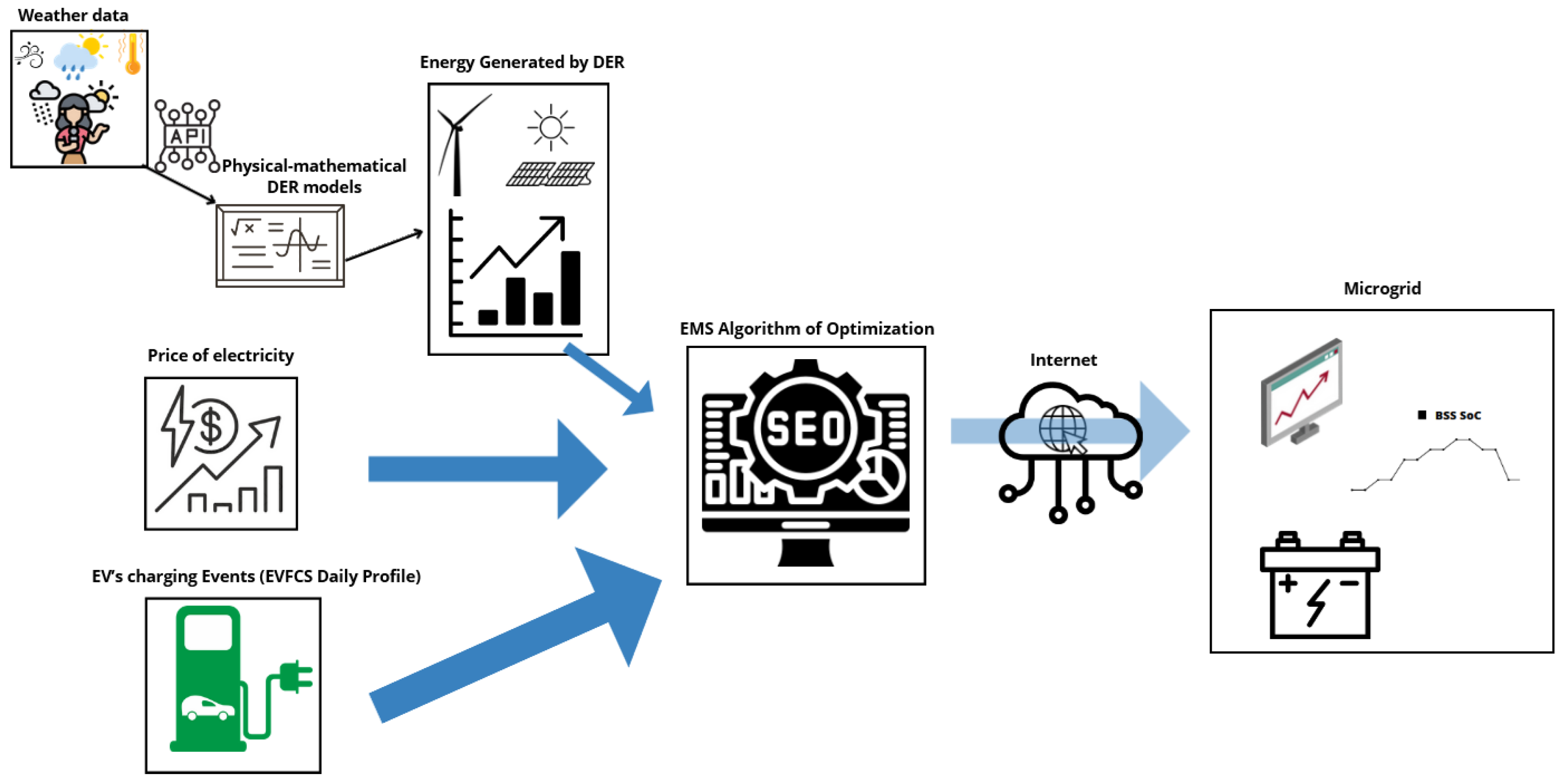
Figure 2.
Schematic process for data collection, analysis, and estimation of daily EVFCS demand profiles.
Figure 2.
Schematic process for data collection, analysis, and estimation of daily EVFCS demand profiles.
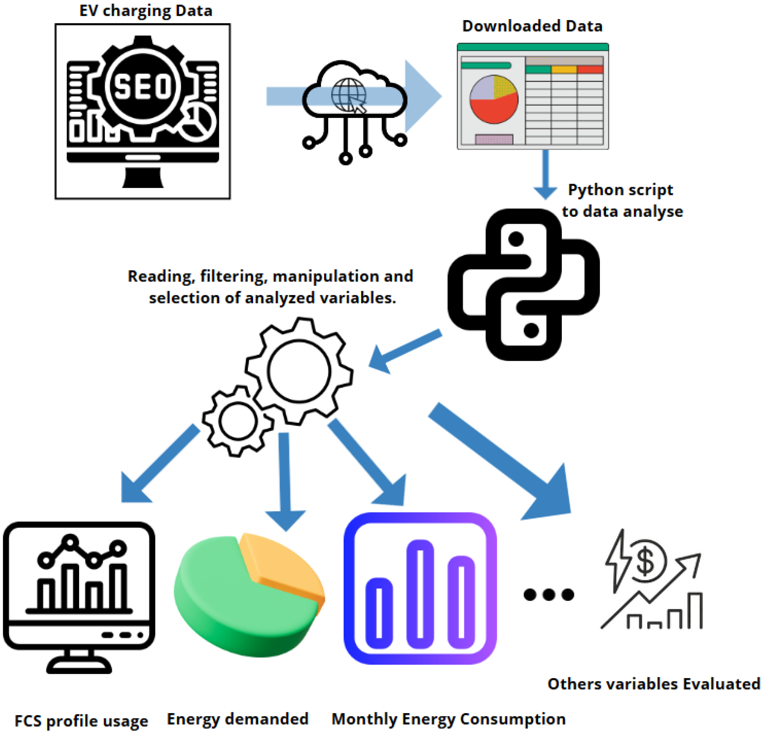
Figure 3.
Example of EVFCS daily charging profile generated by the algorithm.
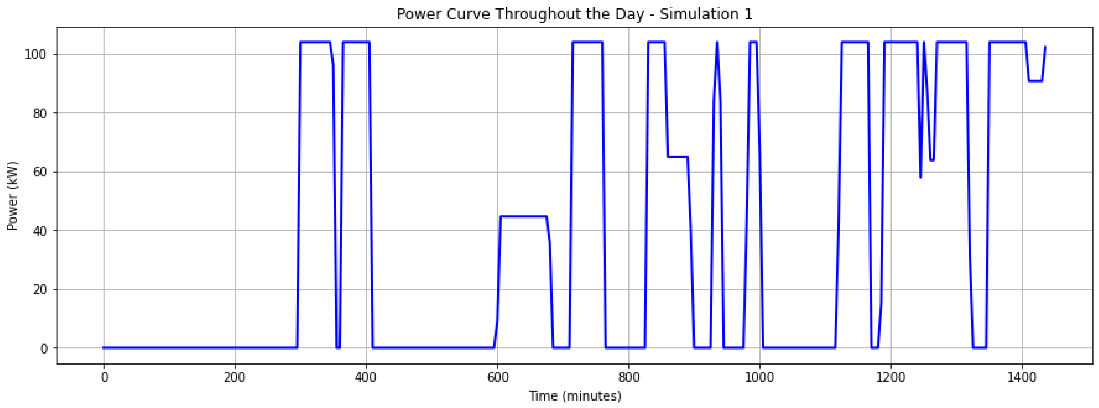
Figure 4.
Power curve vs wind speed for 30 kVA WT.
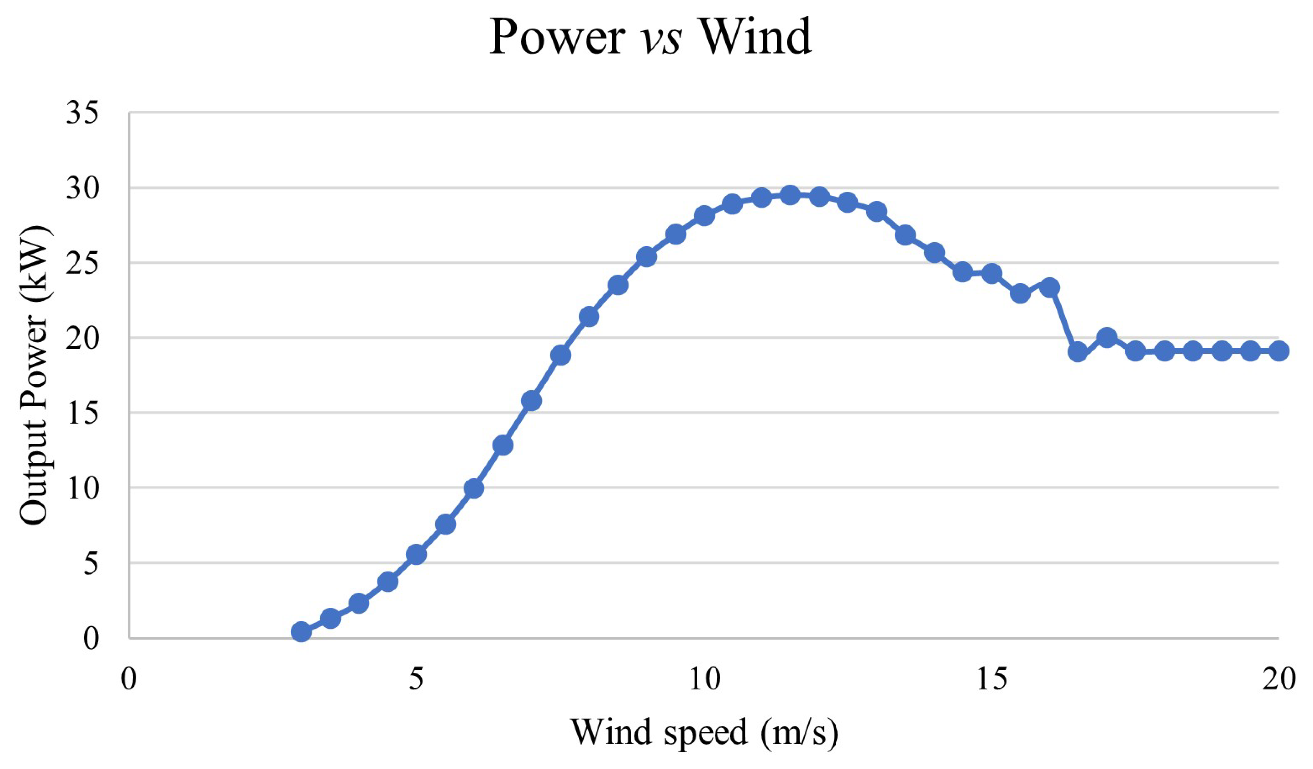
Figure 5.
Flow of obtaining information via API, data processing, application of equations and obtaining the wind generation profile.
Figure 5.
Flow of obtaining information via API, data processing, application of equations and obtaining the wind generation profile.
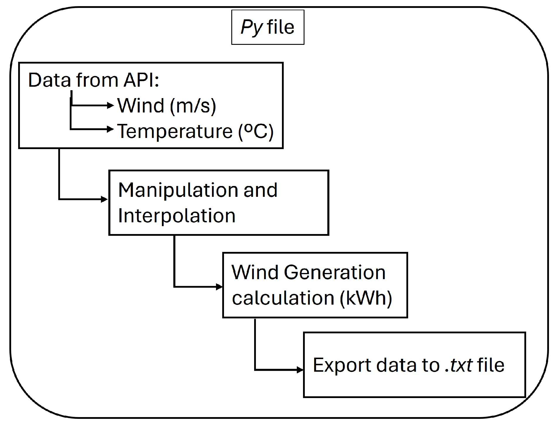
Figure 6.
Flow of obtaining information via API, data processing, application of equations and obtaining the photovoltaic generation profile.
Figure 6.
Flow of obtaining information via API, data processing, application of equations and obtaining the photovoltaic generation profile.
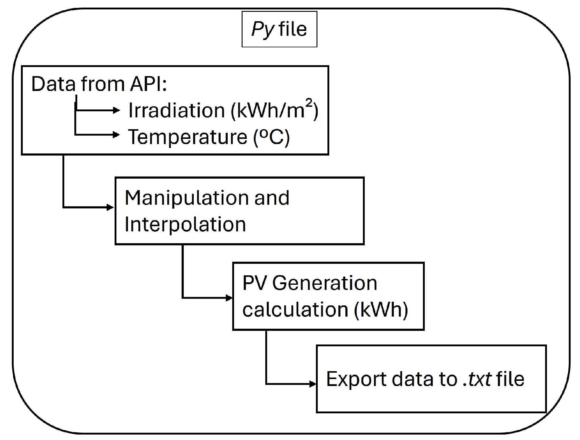
Figure 7.
Scheme of the MG used in the case study.
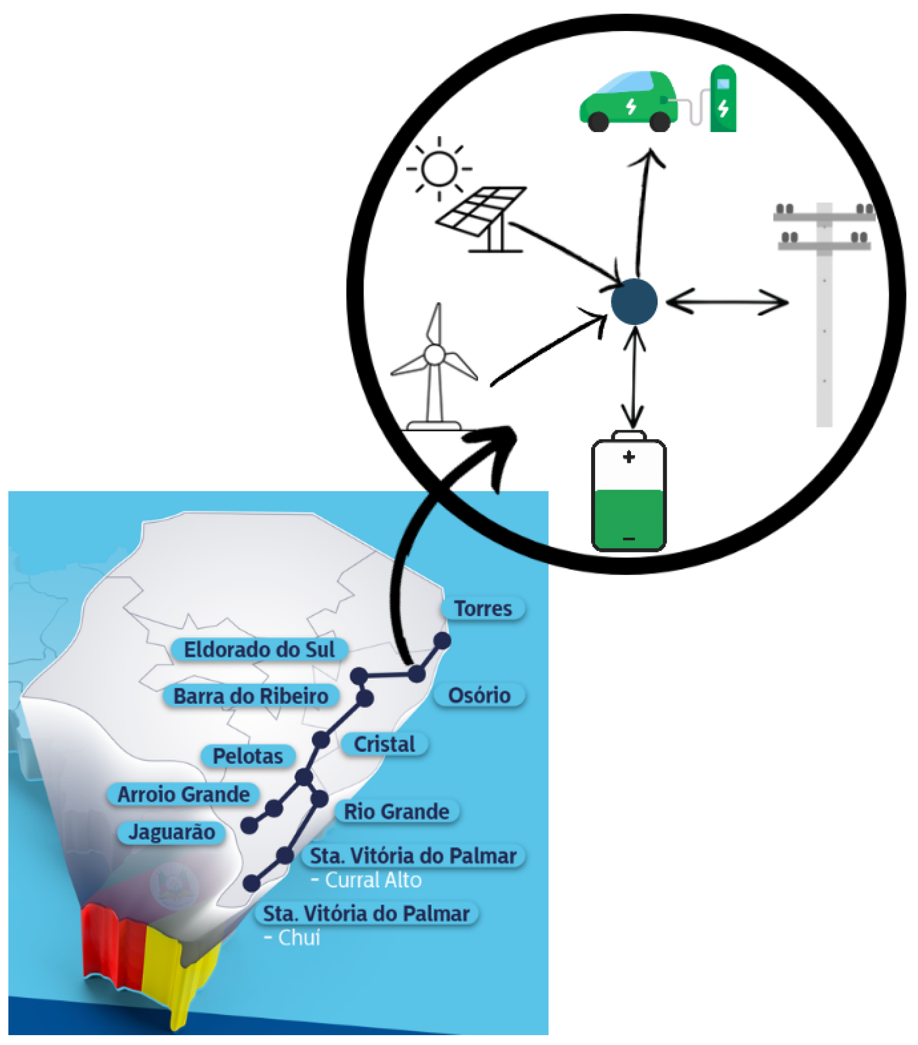
Figure 8.
Equatorial Energia’s White ToU Tariff, valid from 2024 [48].
Figure 8.
Equatorial Energia’s White ToU Tariff, valid from 2024 [48].
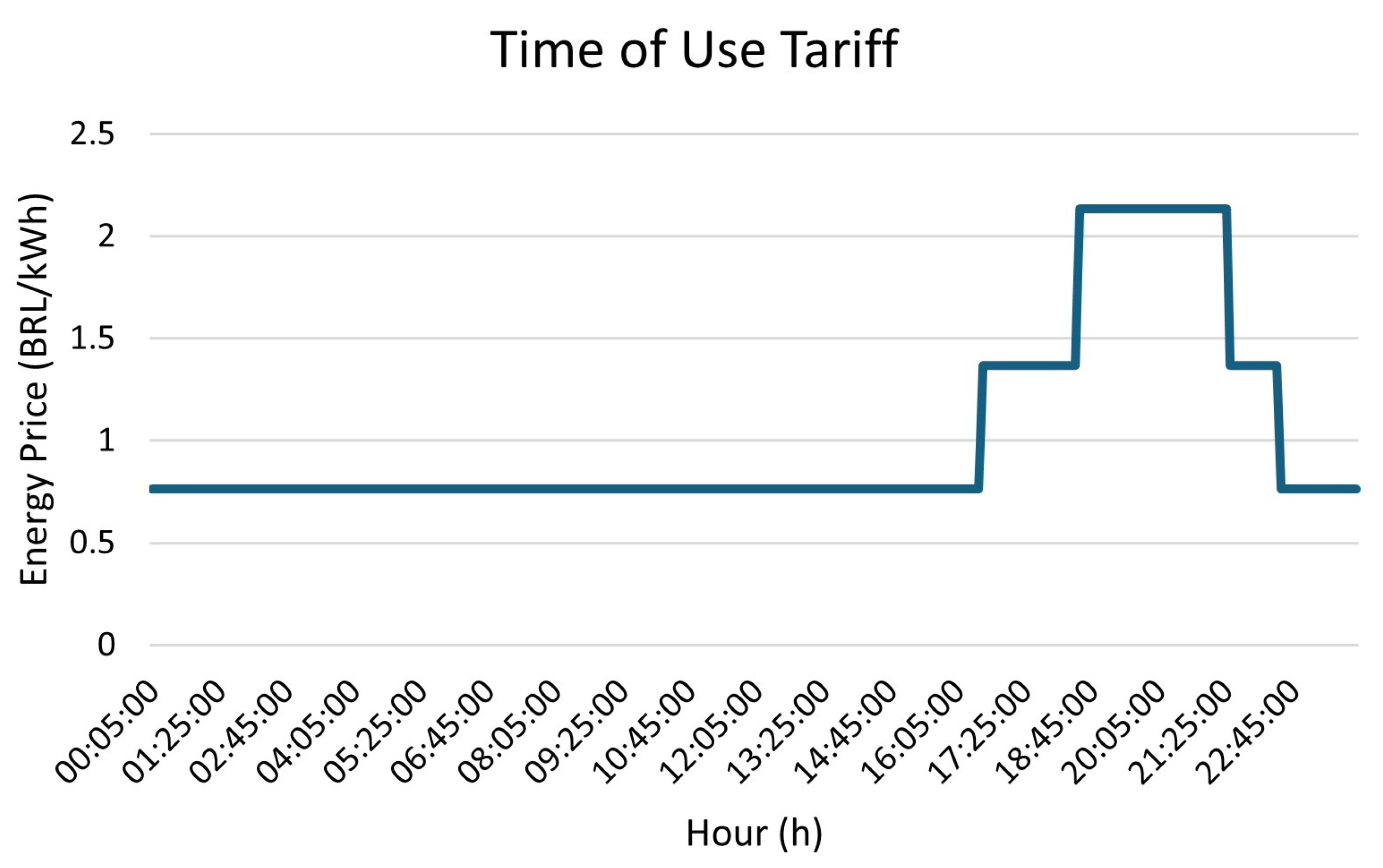
Figure 9.
ACC vs DoD curve of the batteries that compose the BESS [9].
Figure 9.
ACC vs DoD curve of the batteries that compose the BESS [9].
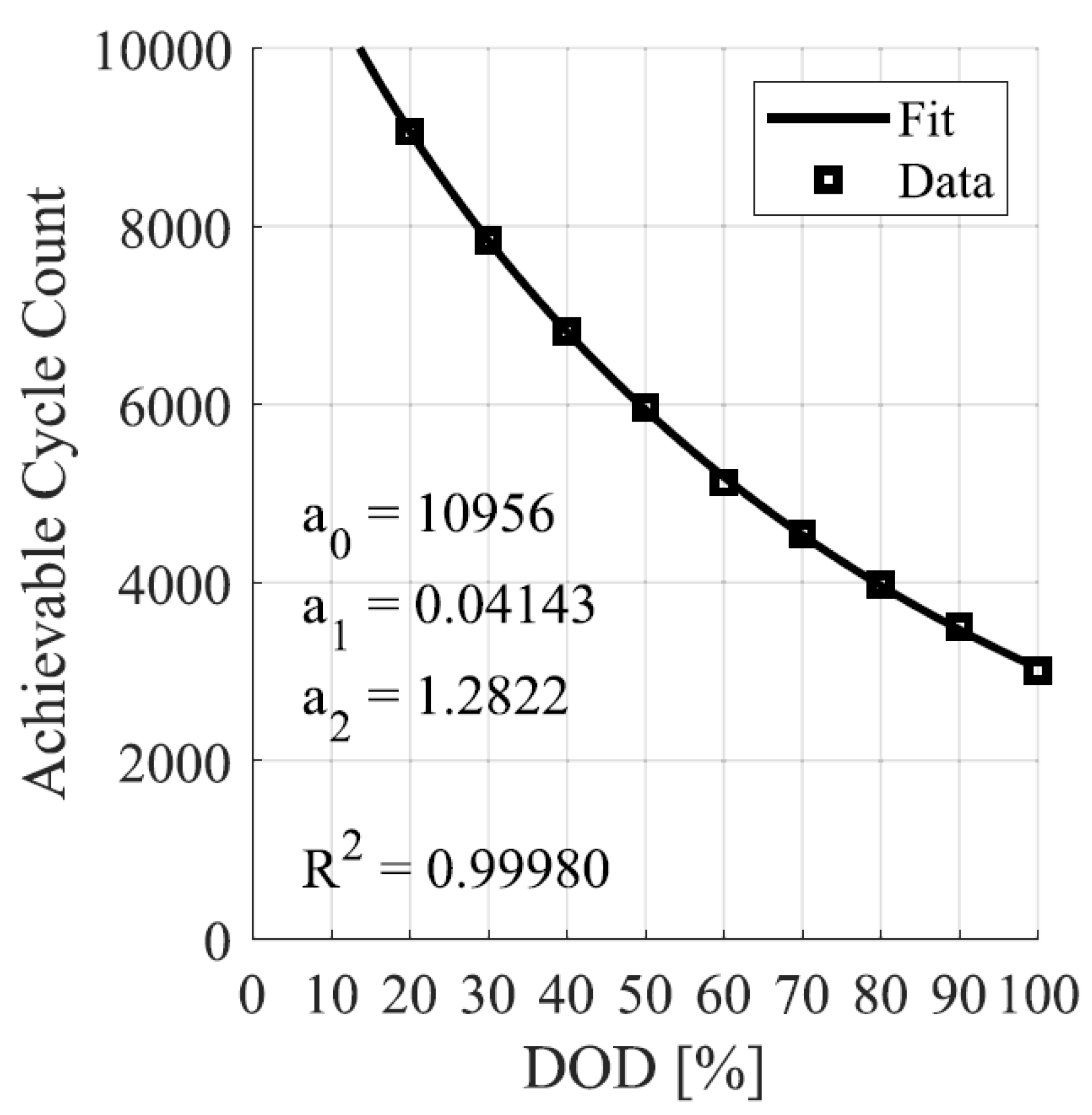
Figure 10.
Wear Density Function of the BESS battery.
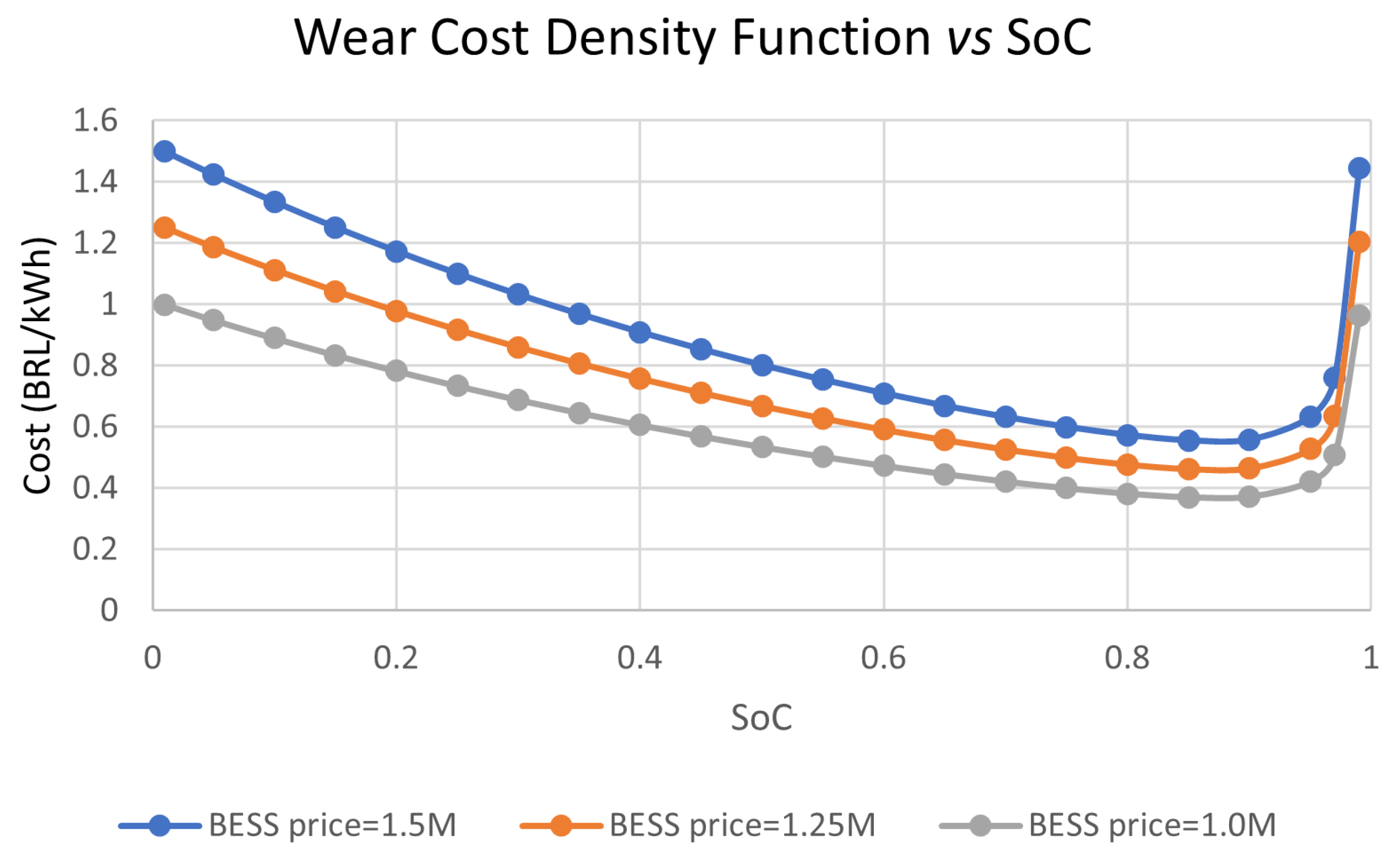
Figure 11.
Example of the Daily Generation Curve of WT and PV.
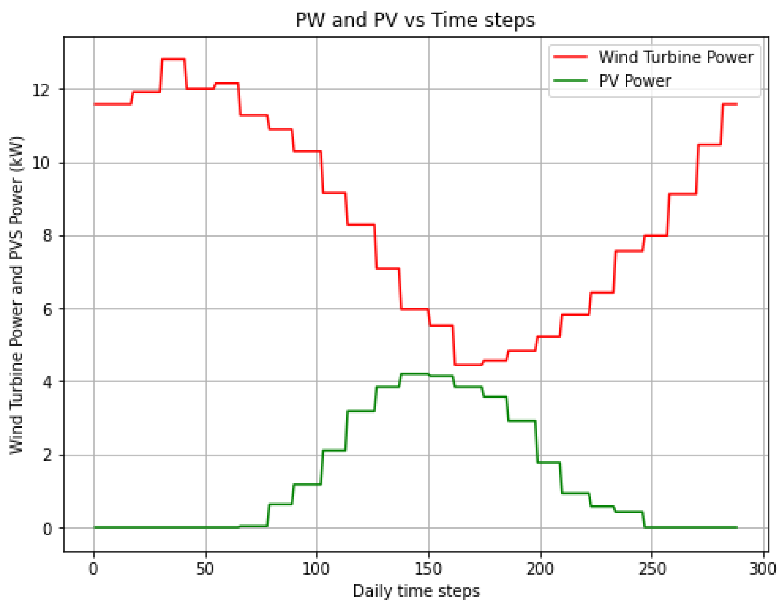
Figure 12.
Histogram of the connection time of EVs in the MG.
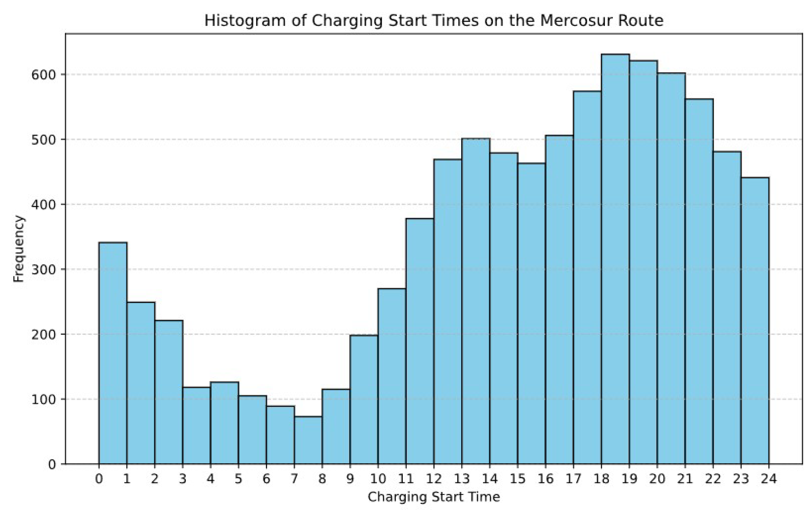
Figure 13.
EVFCS average load curve from 1000 daily simulations.
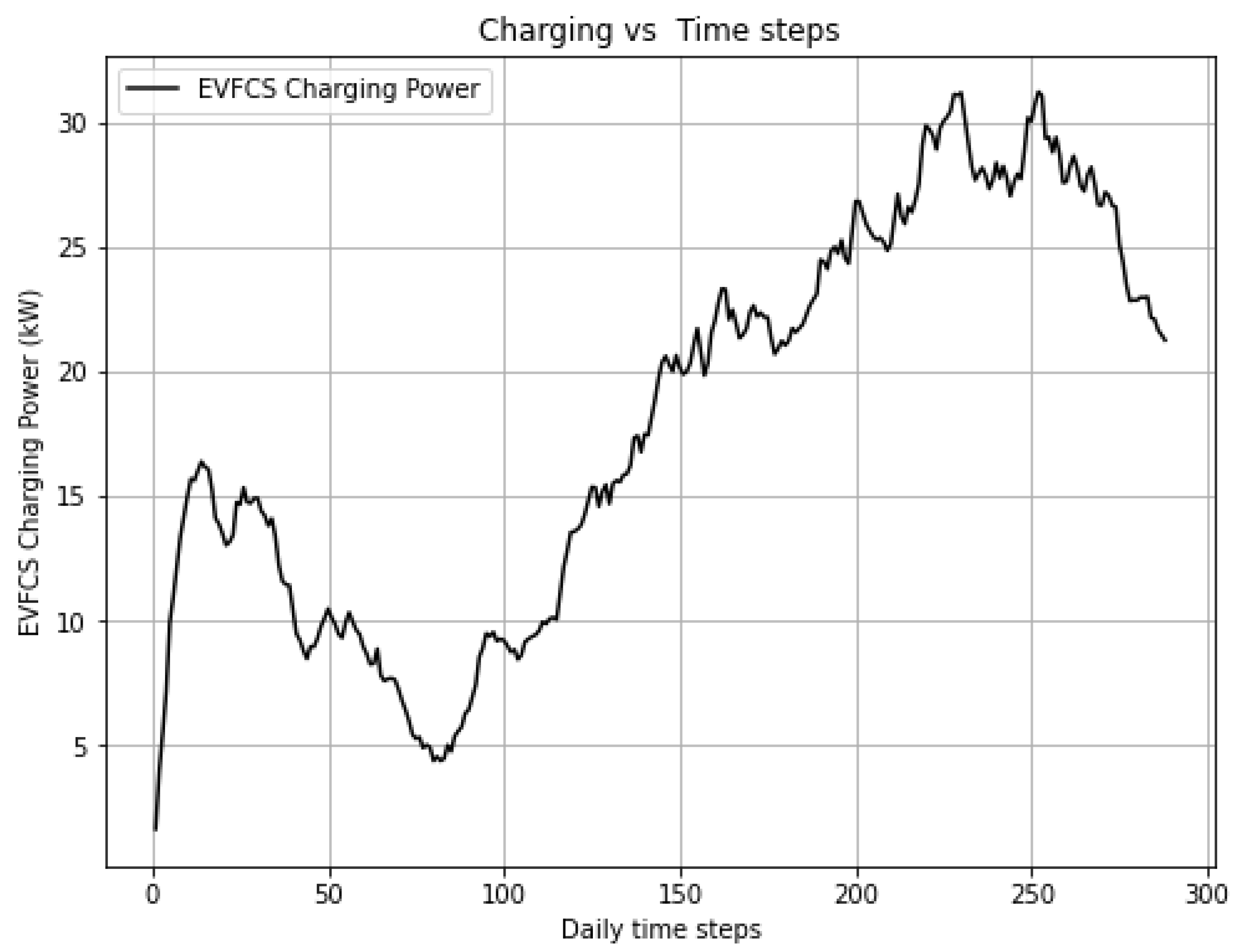
Figure 14.
Daily load simulated to a weekday.
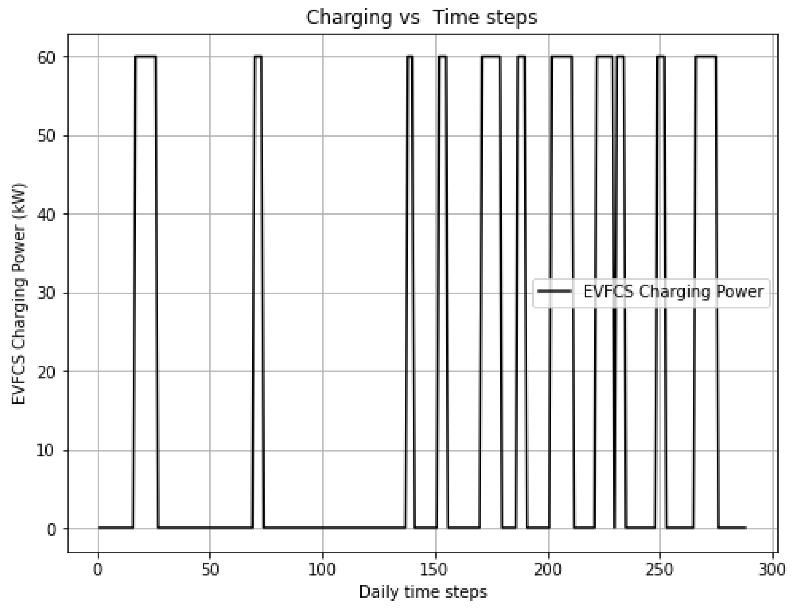
Figure 15.
Daily BESS dispatch.
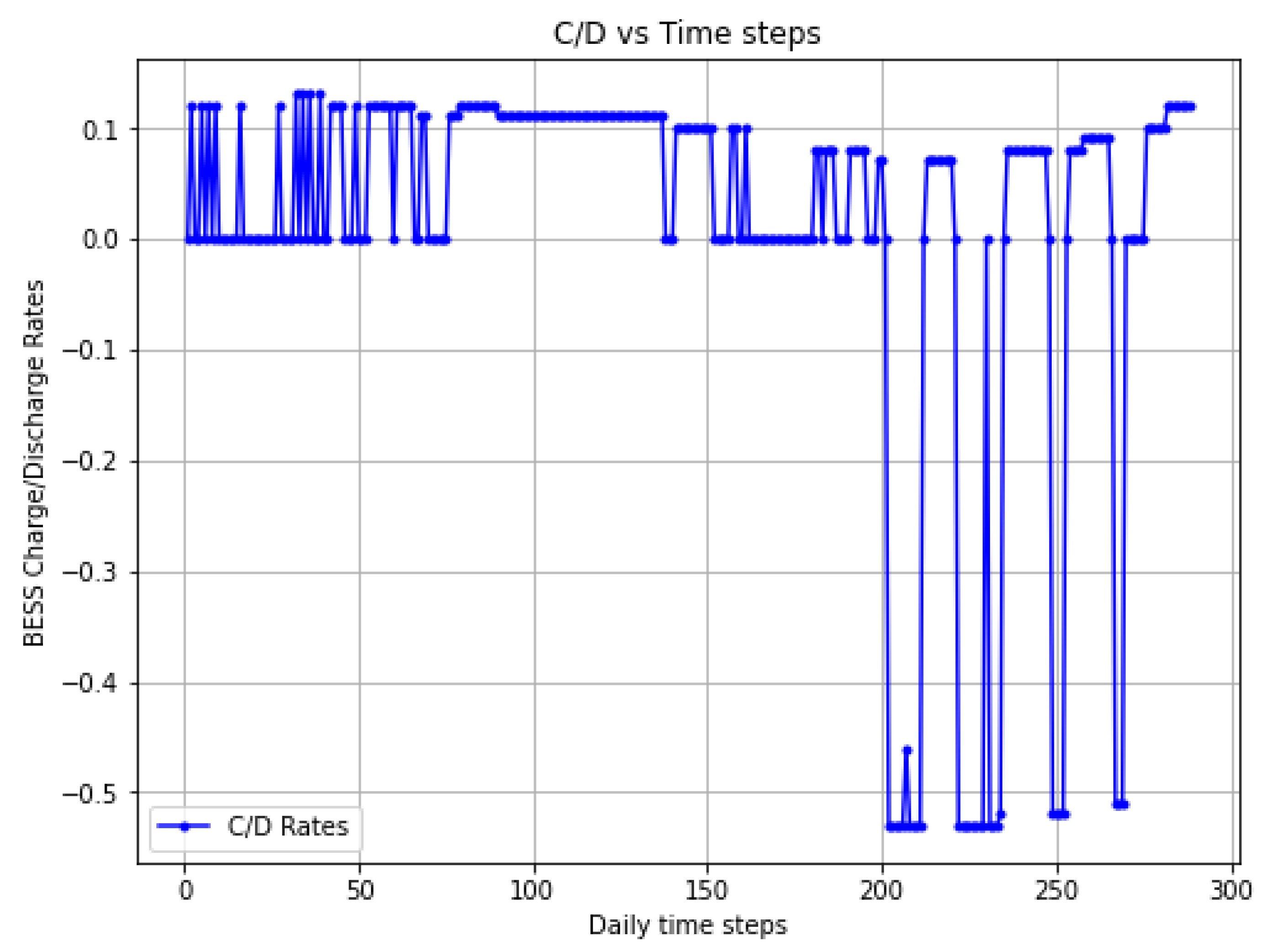

Table 1.
Notation for the optimization problem.
| Type | Name | Description |
|---|---|---|
| Set | T | Time (discretization: to J) |
| Parameter | J | Total number of time intervals (288) |
| Parameter | Ts | Sampling time (discretization of 5 minutes = 0.0833 h) |
| Parameter | Efficiency (0.95) | |
| Parameter | Minimum SoC | |
| Parameter | Maximum SoC | |
| Parameter | Initial SoC of the BESS | |
| Parameter | BESS capacity | |
| Parameter | Maximum charging power of the BESS | |
| Parameter | Maximum discharging power of the BESS | |
| Parameter | Maximum grid power (transformer) | |
| Parameter | Parameter of the ACC(dod) function | |
| Parameter | Parameter of the ACC(dod) function | |
| Parameter | Parameter of the ACC(dod) function | |
| Parameter | Temperature coefficient | |
| Parameter | M | BESS price (1500000) |
| Parameter | BESS capacity | |
| Parameter | Grid injection discount (wire B) | |
| Parameter | EV charging power | |
| Parameter | Energy tariff at instant j | |
| Parameter | Photovoltaic generation profile | |
| Parameter | Wind generation profile | |
| Parameter | BESS wear average cost | |
| Parameter | Total charge cycle and total discharge cycle | |
| Variable | Charging rate | |
| Variable | Discharging rate | |
| Variable | Auxiliary binary parameter (BESS status) | |
| Variable | Auxiliary binary parameter (buy/sell logic) | |
| Variable | SoC calculation | |
| Variable | Power bought from the grid | |
| Variable | Power sold/injected to the grid | |
| Variable | BESS charge | |
| Variable | BESS discharge | |
| Variable | BESS wear density variable as a function of SoC variation | |
| Function | Objective function |
1 This table was elaborated by authors.
Table 2.
ToU of the Equatorial Energia Utility.
| Time Period | Description | Commercial Rate (BRL/kWh) |
|---|---|---|
| Peak Hours | From 6:30 PM to 9:29 PM | 2.13181 |
| Intermediate Hours | From 4:30 PM to 6:29 PM and from 9:30 PM to 10:29 PM | 1.36725 |
| Off-Peak Hours | From 10:30 PM to 4:29 PM and on weekends and national holidays | 0.76227 |
Source: Adapted from [48].
Table 3.
Summary of BESS dispatch considering the average curve of EV recharges in MG.
| Variables | Solver HiGHS, | Solver Snopt, |
|---|---|---|
| Energy Charged (kWh) | 0 | 10.79 |
| Energy Discharged (kWh) | 0 | 9.745 |
| SoC (%) | 0 | 5 |
| Energy Bought (kWh) | 218 | 209.22 |
| Energy Sold (kWh) | 25.48 | 14.67 |
| Energy EVFCS (kWh) | 433.64 | 433.64 |
| Total WT + PVS (kWh) | 240.15 | 240.15 |
| OF (BRL) | 290.75 | 295.55 |
Source: Elaborated by authors.
Table 4.
Summary of BESS dispatches considering a weekday charging curve.
| Variables | Solver HiGHS, | Solver Snopt, |
|---|---|---|
| Energy Charged (kWh) | 139.75 | 140.33 |
| Energy Discharged (kWh) | 126.58 | 85.92 |
| SoC (%) | 52 | 44.00 |
| Energy Bought (kWh) | 171.56 | 212.33 |
| Energy Sold (kWh) | 48.03 | 48.03 |
| Energy EVFCS (kWh) | 350 | 350.00 |
| Total WT + PVS (kWh) | 240.15 | 240.15 |
| OF (BRL) | 441.28 | 369.12 |
Source: Elaborated by authors.
Table 5.
Summary of BESS dispatches considering 3 different BESS cost.
| Case | BESS 1.5 M | BESS 1.25 M | BESS 1.0 M |
|---|---|---|---|
| EVFCS avg load curve, OF | 290.75 | 288.95 | 285.01 |
| Weekday, OF | 441.28 | 392.29 | 341.25 |
Source: Elaborated by authors.
Table 6.
Simulation of BESS dispatch on a weekday, without considering .
| Variables | Solver HiGHS without |
|---|---|
| Energy Charged (kWh) | 183.08 |
| Energy Discharged (kWh) | 164.5 |
| SoC (%) | 55 |
| Energy Bought (kWh) | 133.64 |
| Energy Sold (kWh) | 5.05 |
| Energy EVFCS (kWh) | 350 |
| Total WT + PVS (kWh) | 240.15 |
| OF (BRL) | 102.57 |
Source: Elaborated by authors.
Disclaimer/Publisher’s Note: The statements, opinions and data contained in all publications are solely those of the individual author(s) and contributor(s) and not of MDPI and/or the editor(s). MDPI and/or the editor(s) disclaim responsibility for any injury to people or property resulting from any ideas, methods, instructions or products referred to in the content. |
© 2025 by the authors. Licensee MDPI, Basel, Switzerland. This article is an open access article distributed under the terms and conditions of the Creative Commons Attribution (CC BY) license (http://creativecommons.org/licenses/by/4.0/).
Copyright: This open access article is published under a Creative Commons CC BY 4.0 license, which permit the free download, distribution, and reuse, provided that the author and preprint are cited in any reuse.


