Submitted:
13 December 2024
Posted:
17 December 2024
You are already at the latest version
Abstract
The electricity landscape is constantly evolving, with intermittent and distributed electricity supply causing increased variability and uncertainty. The growth in electric vehicles, and electrification on the demand side, further intensifies this issue. Managing the increasing volatility and uncertainty is of critical importance to secure and minimize costs for the energy supply. Smart neighborhoods offer a promising solution to locally manage the supply and demand of energy, which can ultimately lead to cost savings while addressing intermittency features. This study assesses the impact of different electric vehicle charging strategies on smart grid energy costs, specifically accounting for battery degradation due to cycle depths, state of charge, and uncertainties in charging demand and electricity prices. Employing a comprehensive evaluation framework, the research assesses the impacts of different charging strategies on operational costs and battery degradation. Multi-stage stochastic programming is applied to account for uncertainties in electricity prices and electric vehicle charging demand. The findings demonstrate that smart charging can significantly reduce expected energy costs, achieving a 10\% cost decrease and reducing battery degradation by up to 30\%. We observe that the additional cost reductions from allowing Vehicle-to-Grid supply are small compared to smart charging are small. This means that most benefits are obtainable just by optimized timing of charging itself.
Keywords:
Optimization under uncertainty
; electric vehicles
; charging strategies
; battery degradation modeling
; energy storage
; smart neighbourhoods
1. Introduction
Electricity supply and demand management are becoming increasingly complex. This complexity arises from the increasing contribution of decentralized renewable energy source (RES), like solar and wind power, feeding into local distribution grids [1]. Furthermore, the increase in electricity consumption types, such as electric vehicles, often resulting in high demand peaks, further adds to these challenges [2]. As this trend advances, the integration of distributed RES through optimal energy management within smart buildings and neighborhoods is gaining heightened importance [3,4]. The feasibility of intermittent RES such as solar photovoltaic (PV) as standalone power sources is limited due to the inherent fluctuations in electricity generation [5]. A straightforward solution to address RES intermittency is by using storage units. Co-generation units and (legacy) connections to electricity and heat grids may help balance generation peaks and ease the integration of RES. Dispatchable energy units such as storage units for heat and power, and Combined heat and power (CHP) are especially important in disconnected energy communities [6]. The increased flexibility benefits all actors in the energy system at large; however, it comes at the expense of significant investment costs. Optimal use of storage capacity allows investing in smaller, cheaper units. Moreover, considering battery degradation allows trading off arbitrage opportunities with battery lifetime.
The increasing number of electric vehicles (EVs), most of which are idle over of the time, may have role as a flexible source in terms of shiftable demand and storable supply. Managing charging schedules can be beneficial not only for the charging costs of the EVs but also the operational cost of the entire system. Within this landscape, two distinct paradigms come into focus: passive, uncontrolled charging, and active, flexible charging (e.g., [7]. In uncontrolled strategies, vehicles are charged upon plugging in, charging at their maximum capacity until the battery is fully charged. Conversely, active strategies align with electricity price signals and broader system costs, potentially encompassing battery degradation considerations. Taking active charging a step further is the concept of Vehicle-to-Grid (V2G), which represents the most flexible utilization of EV batteries. V2G allows for discharges too, albeit at the cost of added stress and a reduction in battery lifetime [7].
Battery lifetime consists of two distinct components: calendar life and cycle life, both of which contribute to capacity reduction through chemical and mechanical stresses [8]. For batteries that are used frequently, cycle life is often the key factor affecting lifespan [9]. In contrast, for EV batteries, which may only be charged a few times per week, calendar aging is usually the dominant factor. Avoiding battery degradation in techno-economic models of smart grids or energy systems is commonly achieved by imposing a cost per throughput and establishing (often conservative) boundaries for state of charge (SOC) [10,11]. However, these models often overlook the non-linear increase in aging caused by cycle depth (CD) and other aging factors. This oversight typically results in relatively deep charge-discharge cycles and high resting SOC levels, leading to substantially higher battery degradation than the model predicts. Alternatively, excessively penalizing smaller cycles or setting overly tight SOC boundaries can hinder leveraging arbitrage opportunities due to inter-temporal price differences. Several studies focus specifically on modeling battery degradation. For instance, [9,12] analyzes the impact of degradation on electric vehicle batteries and its associated cost implications. Similarly, [13] investigates the effects of battery degradation in electric vehicles and stationary batteries on the investment costs of distribution networks for renewable energy-based distributed generation, energy storage systems, and electric vehicle charging stations. This study only includes the impacts of depth of discharge on the degradation cost. However, many other studies examining the interplay between EVs and smart neighborhoods oversimplify degradation costs, often reducing them to a constant value [14,15,16,17].
Moreover, the challenge of (foreseeable) intermittency, as well as uncertainty arising from sources such as RES, market prices, and demand, impacts least-cost operation [14,15,18,19]. Uncertainty in electricity prices and demand impacts least-cost operation and is a key challenge in energy systems. For instance, virtual power plants have been proposed to aggregate small-scale battery energy storage systems for frequency regulation, demonstrating how managing uncertainties in market prices and storage degradation is crucial for their operational success [20]. Despite the significant impact of uncertainty, most researchers deploy deterministic models (c.f., [21,22,23]). An exception is [24], who propose a two-stage stochastic model aimed at optimizing the operation of a RES-based micro grid (MG) equipped with an EV parking lot. However, in energy systems, uncertain events typically unfold across multiple temporal instances, making stochastic programs with multiple (more than two) stages more appropriate [25,26]. At present, the number of multi-stage models for operational scheduling in energy systems is relatively limited. Most smart grid literature focuses on deterministic or two-stage stochastic models to deal with optimal operational problems of smart energy neighborhoods [16,17,27]. However, [28] employ a multi-stage stochastic model to enhance energy-efficient scheduling of a CHP unit, PV, heat boiler, and energy storage systems within a building, addressing both electricity and thermal demands. [29] apply stochastic dual dynamic programming and compare a two-stage and a multi-stage model to minimize the expected total cost of an IEEE 118-bus system with integrated RES. Additionally, many papers overlook or simplify the degradation costs associated with stationary storage and EV batteries. With this paper, we aim to contribute to the literature by developing a multi-stage stochastic model of a local energy system with a detailed battery degradation representation.
This paper investigates how electric vehicle charging strategies interact with behavioral and price uncertainties in a building complex equipped with various energy generation and storage options. We aim to minimize expected operational costs, including battery degradation costs. To achieve this, we adopt the improved battery degradation model as developed in [30]. In [30], a battery and a spot market for electricity are the two considered elements. The multi-stage operational model in the current paper considers a system with many more elements, and it provides a comprehensive framework for accommodating uncertainty in EV owners’ behavior (charging demand) and electricity prices.
This study is conducted to assess the impact of different charging strategies for EV on the operational energy costs while taking into account battery degradation. The method is applied to a neighborhood within an urban setting, representing a building complex in Pfreimd, Germany. It consists of four buildings with a total of 80 apartments and approximately 300 residents. The complex has its own energy resources and connections to the main energy grids for power, heat, and natural gas. The buildings are outfitted with PV modules. One of the buildings features a small-scale CHP, a TES, and a stationary battery. External electricity and district heating grids both supply energy to this community, and surplus electricity can be fed back into the grid, however, heat can not. In this analysis, we account for battery degradation in both the stationary battery and the EVs batteries with the representations developed in [30]. We also consider uncertainty in electricity prices and demand. In this study, we consider Nickel Manganese Cobalt (NMC) batteries only due to their widespread usage in electric vehicles [31]. Due to lacking data, other battery types, such as Lithium Iron Phosphate batteries, as promising as they may be in light of sustainability and ethical considerations [32], are not in the scope of the current paper.
In summary, the key contributions of this paper are as follows:
- The interaction between electric vehicle charging strategies, behavioral uncertainty, and price fluctuations in a building complex equipped with various energy generation and storage options is analyzed.
- A comprehensive framework is provided for considering both electric vehicle and stationary battery degradation, based on calendar aging, cycle depth, and SOC levels, in the context of minimizing operational costs.
- A multi-stage stochastic operational model is developed to minimize expected operational costs, including battery degradation costs, by accounting for uncertainty in EV charging demand and electricity prices.
- Three charging strategies — passive charging, smart charging, and V2G charging — are considered to investigate the impact on degradation costs and evaluate the differences in operational energy costs for each strategy.
- We show that smart charging achieves a significant reduction in energy cost and battery degradation, and that most benefits are obtainable just by optimized timing of charging itself; Vehicle-to-Grid delivery adds relatively little value.
The remainder of the paper is structured as follows. In Section 2, we explain the scenario tree structure used to represent uncertainty and present the mathematical formulation of the proposed model, including the cost function, energy balances, and operational constraints of generation units as well as storage facilities. Section 2.4 provides an electric battery degradation model used in the optimization, detailing three degradation mechanisms. Following this, Section 3 discusses numerical results and findings of the conducted case study. Lastly, Section 4 summarizes our findings and identifies future research directions.
2. Model Formulation
In this section, we present the mathematical framework developed to evaluate the impact of EV charging strategies within a complex building environment, as discussed in Section 1. Consider B representing the set of buildings within the complex, with b indexing individual buildings. Each building b has distinct heat and electricity demands. To supply this demand, the model considers two types of grids: local, L, and main, M, and includes three energy carriers within set E: electricity, heat, and gas denoted as respectively. Gas is used exclusively as an input for the CHP. In the following subsection, we begin by introducing the scenario tree structure, a key component for addressing uncertainty.
2.1. Structure of Scenario Trees
To account for stochastic scenarios, we utilize a tree structure. A scenario tree, which features interconnected nodes h, is similar to a decision tree but differs in its branching. A scenario tree branches due to uncertain events, not based on distinct decisions. C.f., Figure 1.
All scenarios start from the root node (the first hour in the planning horizon, node 1 in the example figure, Figure 1), with each scenario leading to a unique terminal node (, a possible realization of the last hour in the planning horizon, c.f., one of the nodes 20-23 in the example figure). In a scenario tree, predecessor and successor nodes determine the possible paths from the root node to all terminal nodes. Each node in the scenario tree has one unique predecessor but may have multiple successors. (E.g., node 6 has predecessor node 4 and successors 8 and 9. We use to denote predecessors. E.g., in Figure 1, is node 4.) A ’stage’ in the tree represents a specific time period and may include several parallel nodes in different scenarios. (E.g., nodes 4 and 5 are both in stage three.) We allocate probabilities to each node and ensure their sum equals 1 in each stage, to enable calculating expected values. This structure systematically represents the outcomes of stochastic variables, enabling decision optimization based on the realization of past information while anticipating future uncertainties.
2.2. Objective Function
The objective function is to minimize expected energy costs Eq. (1).
The initial term within the first bracket represents the cost of purchasing energy from the main grid () at the price of for each building b and energy carrier e at hour h. The second term calculates the feed-in remuneration from injecting energy into the main grids, accounting for transmission losses () and with varying tariffs depending on the energy source. It includes remuneration for RES at a rate of and for CHP generation at a rate of , with associated injections represented by . On the second line, we include the costs of gas for the CHP at price and the operational costs for each produced. Additionally, the term represents the costs associated with battery degradation type w for each building b and hour h. The term on the third line is a penalty for any deviation in SOC levels at the end of the scheduling period from their initial values. In active charging schemes, deviations between the end-of-horizon and starting SOC levels are allowed but penalized by a value 1. This allows flexibility in response to significant electricity price variations at similar hours on different days. Each value is weighted according to its probability, denoted as . Since our planning horizon is short, we do not apply discounting.
2.3. Constraints
This section presents the various types of constraints.
2.3.1. Mass Balances
Eqs. (2) and (3) detail the energy balances for the buildings and local grids, respectively. These balances include electricity and heat, covering the supply from RES and CHP units. They also account for interactions with local and main grids, as well as storage. We factor in grid exchange losses during energy injection. There is no balance for gas; its usage is completely determined by CHP output, as discussed below.
The upper limit for grid injections from is set by the RES production itself, as shown in Eq. (4). The total injections into the main grid are the sum of those from CHP and RES, detailed in Eq. (5). Any excess heat is either stored in the thermal energy storage (TES) or curtailed; it cannot be injected into the main grid (c.f., Eq. (6)).
2.3.2. CHP Unit
To model CHP units and battery storages further down in the paper piecewise linearization is used. Line segments correspond with operating ranges. We apply an approach which means that we use binary variables to select the active operating range, while weighting variables determine the actual operating level on that segment. The line segmentation is defined by breakpoints, including an off state, a minimum operating level, and some other operating levels. Eq. (7) ensures that only one line segment can be active at a time. Eq. (8) ensures that the breakpoint representing the off state can only be active alone. Eq. (9) guarantees that these weights can only be positive for the selected active segment. Finally, Eq. (10) ensures that the sum of the weights determining the operating level equals 1. The energy input and output for CHP units are then defined by Eqs. (11) and (12).
2.3.3. Energy Storage Devices
The stored energy level for both electrical and thermal storages at the start of a time step equals the level of the previous time step adjusted for loss-corrected charges or discharges as indicated by Eq. (13). In this context, denotes the immediate predecessor node of h in the scenario tree. For arriving EVs, the storage level from the previous time-step indicates the SOC upon arrival. To assure a fully charged EV at departure, we impose . For passive charging, we fix appropriate values for charging levels . Naturally, for smart charging and V2G, is determined by the model as part of the cost minimization. While discharges for both passive and smart, for V2G it is a model-determined variable.
In the following, we extend the battery degradation formulation developed in [30], incorporating additional indices to account for a more granular problem setting as well as uncertainty. For non-linear CD based degradation, we follow the approach to apply piecewise linearization on virtual electric battery segments , with equal sizes and segment-specific costs. We do not consider degradation of TES. To get a more succinct presentation, the equations below apply for heat storage with one segment only; .
Eq. (14) enforces storage capacity limits (at the segment-level.)
A storage device can only be in one mode at a time; charging, discharging, or steady state, which is enforced by Eq. (15). Eqs. (16) and (17) restrict the charging and discharging rates to their maximum values. Here, parameter defines the presence of batteries, particularly for EVs that may or may not be connected. For stationary storages , always. Lastly, Eq. (18) determines if the battery is in a steady state.
2.4. Electric Battery Degradation
Variables in Eq. (19) aggregate costs for cycle-depth degradation, SOC-cycle degradation, and calendar degradation. The component-wise relative capacity losses (whose computations are presented below) are added and multiplied by battery replacement unit cost (r) and the rated battery capacity (). To be explicit, the subscript ’’ is used in Eqs. (19)-(37) to denote that only degradation is considered for the electricity battery.
2.4.1. Cycle Depth Degradation
CD aging accounts for the degradation on a battery due to repeated discharging cycles, with the degradation rate increasing nonlinearly with deeper discharges. A cycle counting mechanism, such as the rainflow algorithm, is employed to identify and measure these cycles, ensuring consecutive discharges within the same cycle are aggregated appropriately [33]. The CD degradation model used in this study is based on a piecewise linear stress function based on material stress properties, as shown in Eq. (20) [30,34]. This function captures the relationship between capacity loss per cycle and the depth of discharge, where a is the maximum capacity loss per cycle and m is the fatigue strength exponent:
In this paper, the CD-based degradation after each discharging period is computed using a piecewise linear approximation, as defined in Eq. (21). In this equation the first term determines the amount discharged from each battery segment during the time step, normalized by the segment’s rated energy. The second term calculates the relative degradation for the segment using the stress function , effectively summing the degradation contributions across all segments:
By combining a robust cycle counting mechanism with the piecewise linear degradation model, this approach enables accurate computation of capacity loss for each segment, providing a detailed and implementable framework for battery aging analysis. For more details, refer to [30].
2.4.2. Average Cycle SOC Degradation
SOC-based aging requires auxiliary values that are used to impose a penalty at the end of each discharge cycle. Eq. (22) computes the relative SOC compared to battery capacity. This model and the corresponding constraints are adapted from [30].
Eqs. (23)-(25) and (26)-(28) determine the start and end points of specific discharging cycles, respectively.
The binary variables and represent the start and end of a discharge cycle, respectively. Next, Eqs. (29)-(32) compute and penalize the average deviation from 50% SOC within each discharge cycle.
represents the SOC level at the start of a discharge cycle. This is calculated by considering the current SOC and the binary variables indicating the start and end of the cycle. measures the average deviation from an (optimal) 50% SOC level during each cycle. Lastly, Eq. (32) uses these deviations to calculate the SOC-based degradation cost , highlighting the economic implications of SOC fluctuations on battery lifetime.
2.4.3. Calendar Degradation
Calendar aging depends on factors such as time, ambient temperature, and the state of charge, with prolonged periods at high SOC levels accelerating degradation. In this work, the calendar degradation model builds on the approach presented in [30], incorporating an empirically derived degradation rate for lithium-ion batteries as described in [35].
Eq. (33) ensures that only one line segment is active at a time. Eq. (34) ensures that only the weights for the active line segment can be positive. Eq. (35) guarantees that the weights sum to 1. Eq. (36) determines for an SOC level the weight factors on the relevant line segment. Lastly, the calendar degradation value is calculated using Eq. (37).
This concludes the presentation of the model formulation. The next section provides the input data description for the executed numerical experiments.
3. Numerical Results and Discussion
First, we present a set of deterministic cases to provide a clear understanding of the operational dynamics of the system when accounting for battery degradation and a specific charging scheme. Next, we consider uncertainty in grid electricity prices and demand through varying the SOC of EV batteries when they arrive at the building complex to be recharged. All cases are solved using Pyomo with Gurobi version 9.1.2 [36]. The solution time for the deterministic cases is between one and two minutes each on a regular desktop computer with specifications: Intel(R) Core(TM) i5-6200U CPU @ 2.30GHz 2.40 GHz Processor with 8 GB RAM.
3.1. Input Data
The building complex is modeled based on an existing complex in Pfreimd, Germany. Apart from the local grid between the buildings, the buildings are connected to the main grids for electricity, gas, and district heating. We introduce a stationary electric battery and EV charging stations to the setup. We consider an hourly time resolution. For the analysis, we have selected a day late in Spring, Monday, June 3, 2019, when the complex had a peak electricity demand of 68 and a peak heat demand of 43 . The PV peak generation was 73 . (For most other parts of the year, the solar panels generate less electricity and the heat demand is high. In such cases, the CHP runs the entire day, which makes the operational dynamics uninteresting. In contrast, in the hottest summer months, heat demand is negligible and solar generation high, which results in very low to no CHP operation.) Appendix A.1 details hourly input data of electricity price, electricity and heat demand, and PV generation of the building complex.
Table 1 presents the CHP output and efficiency for four different operation modes, which form the breakpoints of the piecewise linear segments. Table 2 displays the storage data. We include six EV with battery dimensions of a Nissan Leaf and replacement cost r at 150 €/. All degradation data is for NMC batteries. The values for CD parameters a, m, and f are sourced from [30,37]. Calendar degradation parameters are based on [38] with four segments reported in Table 3.
Hourly electricity prices are German spot prices for Monday, June 3, 2019; we add the network fee ( ¢/ [39]) and value-added tax (). The gas price is constant at ¢/ and the heat price is 8 ¢/. The CHP has operational costs of ¢/. PV power can be fed into the main grid at a sales price of ¢/ independent of time [40]. Electricity generated by CHP can be fed in at the prevailing spot price.
We consider three EV groups with two cars each, and respective arrival times: 16:00, 17:00, and 20:00, and respective SOC levels upon arrival of , , and .
3.2. Deterministic Case
We consider EV charging strategies passive, smart, and V2G.
3.2.1. Passive Charging
Figure 2a displays own electricity generation, battery discharges, and grid imports as positive values, while demand, battery charges, and grid exports are indicated by negative values. At the start of the day, from 0:00 to 3:00, the CHP runs at full capacity, then slightly reduces its output until 5:00 when solar generation begins, and continues to operate at a lower capacity until 9:00. As such, the CHP covers most of the electricity and the entire heat demand during the night, while also charging the TES. By assumption, at both the start and the end of the day, the TES is at exactly of its capacity. Charging by the CHP brings the TES to capacity (see Figure 2b), enabling it to meet the heat demand between 09:00 and 15:00. No CHP generated electricity is sold to the grid at any time.
After 9:00, PV generation continues to rise, and the CHP shuts down. Surplus PV power is used for two purposes. First, some is sold to the main grid. Here we note that due to the fixed feed-in remuneration per , the specific selling hour does not matter. Second, batteries are charged. The feed-in tariff is lower than the lowest hourly purchasing price from the grid, making storage for own use attractive. The stationary battery is charged gradually over the day, with a substantial charge to reach the maximum SOC right before the arrival of the first EVs. With grid prices declining gradually between 7:00 and 16:00, the charging schedule is optimized to minimize both costs and calendar aging by keeping the battery at a low SOC during most of the day.
Figure 2c shows the SOC profiles of all battery groups. By assumption, the start and end SOC levels of the stationary battery are . For EVs an SOC of zero indicates that they are not present. The initial SOC levels of EVs at 0:00 equals their respective levels at 24:00.
During the entire evening, there is a high residential and EV demand. With passive charging, as soon as an EV connects, it starts charging at maximum capacity. Additionally, PV generation declines rapidly after 18:00, leading to a spike in grid imports around 20:00 when electricity prices are at their highest for the day. Therefore, while the EV batteries are charging, the stationary battery discharges during these hours to avoid import costs from the main grid. Car groups EV1 and EV2 charge until they are full at 20.00. They both start the next day at , while EV3 starts the day at and charges for one more hour to reach . Due to the passive charging strategy, the charging cannot be postponed until later hours with lower prices.
EV demand is about of total electricity demand, however the cost increase to meet this additional load is almost (increasing from €66.86 to €86.45). Unfortunately, the Passive charging strategy imposes that EVs are charged to a large extent when electricity prices are highest.
3.2.2. Smart Charging
Here, we allow the model to determine when to charge the EVs, given the same charges arrival SOC levels as above, and also impose a full charge upon departure. All other parameter values stay the same.
Figure 3a shows a significant change in the charging schedule compared to passive charging. The earliest arriving EV1 charge for an hour from 16:00-17:00 right after arrival. The other EVs do not charge in the evening and start the day with their arrival SOC from the day before. All EVs charge during the lowest price period between 02:00 and 05:00. (At the main grid or system scale, this can be considered to be filling the valley). Locally, this shift has two benefits. The EVs charge at the lowest electricity price and as the SOC is lower for much of the night it also reduces calendar aging significantly. Table 4 shows that the annualized battery degradation is reduced by , from to .
3.2.3. V2G Charging
Here, we allow the model to decide when EVs charge, but also allow discharge. (We impose a minimum SOC at 0:00 and 24:00 to for all batteries.) Overall, the hourly electricity balance is very similar to that of smart charging. The battery charging hours are all the same. The major difference is in the evening, when EV1 discharges from 19:00 to 21:00. Thereby, it reduces the grid imports during the period of the day with the highest prices. Additionally, EV3 discharges in the last hour of the day (not visible in the figure) and recharges using cheap PV between 06:00 and 09:00 in the morning. Compared to smart charging, the reduction in total system costs from V2G is very small, while EV battery degradation increases by due to the discharges. The operational dynamics of our case study with deterministic data are logical, as shown in Figure 4, and can help to appreciate the results obtained from the case study with uncertainty in prices and EVs charge demand in the next section.
3.3. Stochastic Case
We explore the effects of two sources of uncertainty: EV arrival SOCs and electricity price. We consider three moments during the day where uncertainty is revealed. Two for prices, and one for charge demand. At each price branching point in the scenario tree, we consider upward and downward deviations of compared to the average value in the medium scenario. We assign a probability of to the medium scenario, whereas both the low and high outcome scenarios have a probability. Price uncertainty during the middle part of the day would not have much impact, as the EVs are not connected, and surplus PV generation is sold at a fixed feed-in tariff. We have chosen to let price branches occur at 05:00 in the morning, and 20:00 in the evening, based on battery activity and price levels in the deterministic cases. The price deviations are additive, resulting in five different price levels after 20:00, varying from to compared to average values (c.f., Figure 5). The probabilities corresponding to these scenarios are documented in Appendix A.2.
We assume that the branching on demand uncertainty, defined by the EVs arrival SOC happens at 16:00, despite EV2 arriving one hour later. EV1 and EV2 have expected arrival SOC levels of and respectively, that occur with a probability of . With probability, EV1-EV2 can arrive both with 8 kWh higher or lower combined SOC level (The volume uncertainty is therefore kWh, which is of total battery capacity). We ignore SOC uncertainty for EV3 as we have seen in the deterministic cases that its late departure time in the morning allows charging in the morning hours using cheap power, and to limit the number of scenarios to reduce the needed time to find model solutions. To further reduce the needed solution time, in the following analysis, we have deactivated the functionality to compute (Eqs. (23)-(32)), as this affects the solution time very much, but it is the degradation component with the least impact on the total degradation. We consider three different SOC-level and five price scenarios, which combined results in 15 scenarios in total. We define scenario identification codes PXN. The first letter represents the first price branch, the second letter is the arrival SOC branch, with both three possibilities: low (L), medium (M), or high (H). The third symbol is the number for the second price branch, where 1 is the lowest and 5 highest (c.f., Figure 5). Thus, “LL1” is the scenario: low first price, low arrival SOC, low second price. Also, “MM3” is the expected value scenario. The scenario tree is illustrated in Figure 6, providing an overview of the 15 scenarios covering a 24-hour period. To reduce the length of the analysis, we illustrate the system behavior by contrasting the results of five selected scenarios only. We emphasize that all 15 scenarios are solved simultaneously at once, which means that decisions early in the day are made anticipating all possible scenarios later in the day.
Again, we evaluate the three different charging strategies, but now considering uncertainty in prices and charge demand. The solution time for each stochastic case is several hours.
3.3.1. Stochastic—Passive Charging
EVs have to charge at maximum power as soon as they arrive, until they are fully charged. Consequently, different charging patterns constitute a shorter or longer charge period and are due only to different arrival SOC (These results are not shown in a figure). Not only EVs battery charges, but also stationary battery charge and discharge vary dependent on the scenario. Firstly, the first price branch at 05:00 leads to three SOC paths. In all scenarios when prices between 5:00 and 20:00 are lower than average, “LXN”, the stationary battery reaches a maximum SOC of during the day, in all “MXN” scenarios , and in all “HXN” scenarios . The effect of uncertainty is that in most cases the battery charges significantly more than in the deterministic case. In all scenarios, stationary battery discharges start at 19:00, when the period starts with the highest electricity prices.
3.3.2. Stochastic—Smart Charging
Figure 7 shows the stationary battery SOC levels for smart charging for the hours between 13:00 and 23:00, with the three maximum levels the same as for passive charging, and the same time of day to start stationary battery discharges, 19:00. EV2-EV3 charge in the morning, while EV1 charges the same amount of PV power from 16:00-17:00 in all scenarios (See Figure 8). Between 19:00 and 21:00, the stationary battery discharges (until its minimum level of ) to supply residential demand. Thus, for smart charging, the arrival SOC and the second price level, do not affect battery operation compared to passive charging.
3.3.3. Stochastic—Vehicle to Grid
Under V2G charging, the stationary battery profile closely resembles the smart charging profile, but with some distinctions arising from EV discharges. As depicted in Figure 9 which shows EV1 SOC profiles between 16:00 and 23.00, in scenarios with above average prices, EV1 begins discharging at 19:00, while in scenarios with continuing low prices in the evening no discharges occur. The stored electricity is saved for the next day. EV2 engage exclusively in discharging in the “HH5” scenario with consistently high prices, as illustrated in Figure 10.
We observe that the discharge schedules prioritize utilization of the stationary battery, and is driven more by price differences than by battery degradation. EVs discharge can be beneficial if they arrive early enough to charge with cheap PV power. However, in most situations, PV, CHP, and the stationary battery are cheaper supply options to meet demand. However, if EV discharges are used, they reduce the degradation of the stationary battery.
3.3.4. Cost Comparison
Figure 11 presents the system cost for the three charging schemes. It shows that CHP costs are the same in all scenarios, and form the main part of the total cost. In contrast, grid exchange costs vary significantly. Naturally, net import costs from the main grid are lowest in the low price scenario “LL1” and highest in the high price scenario “HH5”. Especially in scenarios with high electricity prices early on (“HXN”), battery degradation costs are relatively high due to high battery discharges to mitigate some of the high price consequences. Battery degradation is up to of total costs in some scenarios, which is substantial, and highlights the importance of trading off degradation costs and the grid electricity price variations. Considering that CHP costs are such a large component, the relative share of battery degradation cost may be even higher in a set up relying completely on RES. Interestingly, in the middle ground scenario “MM3”, the V2G charging scheme reduces expected overall costs by compared to smart charging, much more than in the deterministic case. The added flexibility has higher value when uncertainty is considered. Furthermore, due to the rather modest price variations over the day, the stationary battery cycles only once, which limits the impact of degradation and the interplay with EV charging and discharging. For all charging schemes, calendar degradation is the primary EV battery degradation factor in this analysis, while for the stationary battery, CD degradation is the biggest contributor. Higher price volatility and uncertainty would possibly lead to higher degradation costs, while at the same time reducing total energy costs.
In the middle ground scenario “MM3”, the V2G scheme reduces overall costs by compared to smart charging, much more than in the deterministic case.
4. Conclusions
We have developed a novel optimization model that can easily be parameterized to analyse and optimize smart-energy building complexes and neighborhoods. We have examined the impact of different charging strategies for EV batteries under demand and price uncertainties while considering a detailed model for battery degradation. This analysis focuses on how charging strategies affect the overall operational energy cost within a smart urban neighborhood. Our results show an about cost decrease from smart charging compared to passive charging. This reduction is mainly achieved by shifting the charging time frame from the expensive evening period to the early morning hours with lower prices. This delayed charging also reduces EV battery degradation, with reductions of up to . When considering V2G and allowing EV discharges, total system costs hardly reduce further compared to smart charging, as the modest direct energy cost decrease is partly undone by higher degradation costs. However, uncertainty in electricity prices and EV arrival SOCs allows a more significant cost improvement of V2G compared to smart charging. Its increased flexibility makes V2G cheaper than smart charging.
Battery degradation is up to of total costs in some scenarios, which is substantial, and highlights the importance of accurately trading off degradation costs and grid electricity price variations.
Smart management of a building complex reduces demand in high price periods and increases demand in lower price periods. This provides value to the energy system and society at large, increasing utilization of cheaper generation options, and allowing higher-value utilization of generated electricity by other sources.
The flexibility of V2G is likely to become increasingly beneficial in a future with much more renewable electricity supply and potentially more volatile prices. As suggested by [41], benefiting from demand shifting should not rely on manual actions and be automated as much as possible. Artificial intelligence will play a key-role in customizing charging patterns for specific users and situations through real-time monitoring of battery degradation [42,43] Apps and bidirectional charging equipment should empower consumers to easily or automatically set, accept or override suggested charge-discharge patterns, resulting in lower energy bills, and contributing to higher system efficiency.
Future work may consider degradation of other distributed energy resources such as a CHP and TES. Moreover, employing decomposition methods could shorten solution times and enable the examination of extended scheduling periods.
Abbreviations
The following abbreviations are used in this manuscript:
| CHP | Combined Heat and Power |
| CD | Cycle Depth |
| EV | Electric Vehicle |
| MG | Micro Grid |
| PV | Photovoltaic |
| RES | Renewable Energy Sources |
| SOC | State of Charge |
| TES | Thermal Energy Storage |
| V2G | Vehicle-to-Grid |
| NMC | Nickel Manganese Cobalt |
Nomenclature
Sets andindices:
| Index set | Description |
| Buildings index | |
| Energy carriers electricity, heat, and gas: | |
| Stochastic scenario tree nodes | |
| Predecessor scenario tree node of h | |
| Terminal nodes of scenarios | |
| EV arrival time scenario node index | |
| EV departure time scenario node index | |
| Calendar aging breakpoints | |
| (Virtual) segments in storages of type e | |
| Grid types (main and local grids): | |
| Renewable generation technologies | |
| CHP line segment breakpoints | |
| Storage types, stationary or EVs: |
Abbreviations
| Variable | Description |
| SOC level at the start of the charging cycle. | |
| Deviation to 50% of SOC. | |
| Binary, battery charge mode. | |
| Binary, SOS2 battery calendar aging. | |
| Binary, SOS2 CHP operation. | |
| Binary, battery discharge mode. | |
| Binary, end of a discharge cycle. | |
| Binary, battery steady-state. | |
| Binary, start of a discharge cycle. | |
| Battery charge. | |
| CHP energy input (where ). | |
| CHP energy output (where ). | |
| Generation curtailment. | |
| Battery discharge. | |
| Grid extractions. | |
| Grid injections. | |
| Main grid injections, generated by CHP. | |
| Main grid injections, generated by RES. | |
| Collected cost of electric battery degradation (where ). | |
| Calendar aging-based battery capacity loss (where ) [%]. |
| Cycle depth-based battery capacity loss (where ) [%]. | |
| Average cycle SOC-based battery capacity loss (where ) [%]. | |
| Storage level. | |
| State of charge [%] (where ). | |
| SOS2 segment breakpoint weight for CHP operation. | |
| SOS2 segment breakpoint weight for battery aging (where ). |
Parameters
| Parameter | Description |
| EV connected to charger. | |
| Scenario probability. | |
| Maximum charge rate (where ). | |
| Maximum discharge rate (where ). | |
| Residential energy demand (where ). | |
| Rated energy of the storage (where ). | |
| f | Fitting parameter for average SOC stress of storage. |
| Renewable energy production (where ). | |
| Operational costs of CHP. | |
| Deviation penalty of end-of-horizon SOC-level’s storage. | |
| Grid import price (where ) [€/kWh]. | |
| Feed-in tariff CHP power [€/kWh]. | |
| Gas price [€/kWh]. | |
| Feed-in tariff RES power [€/kWh]. | |
| r | Replacement cost of the battery [€/kWh]. |
| Calendar aging breakpoint (where ). | |
| Breakpoint value CHP gas intake. | |
| Breakpoint value CHP energy generation (where ). | |
| Storage charging efficiency (where ). | |
| Storage discharging efficiency (where ). | |
| Grid injection efficiency (where ). | |
| Breakpoint value calendar aging (where ). |
Appendix A Hourly Data and Scenario Specifics
This appendix includes the hourly data and scenario specifics.
Appendix A.1. Hourly Data and PV Generation
Table A1 lists the hourly demand and PV generation data for the building complex and the spot price of electricity for June 3, 2019.

Table A1.
Hourly data for demand, PV generation, and electricity prices (including network charges and VAT).
Table A1.
Hourly data for demand, PV generation, and electricity prices (including network charges and VAT).
| Time | Electricity price [€/kWh] | Total electricity demand [kW] | Total heat demand [kW] | PV generation [kW] |
|---|---|---|---|---|
| 0 | 0.120 | 26.479 | 23.245 | 00.000 |
| 1 | 0.116 | 24.282 | 30.809 | 00.000 |
| 2 | 0.113 | 23.337 | 39.999 | 00.000 |
| 3 | 0.112 | 19.982 | 41.164 | 00.000 |
| 4 | 0.111 | 19.140 | 43.635 | 00.000 |
| 5 | 0.117 | 20.185 | 29.156 | 00.001 |
| 6 | 0.136 | 26.059 | 27.257 | 08.926 |
| 7 | 0.141 | 26.390 | 23.605 | 25.874 |
| 8 | 0.142 | 32.282 | 24.549 | 40.363 |
| 9 | 0.138 | 33.548 | 19.357 | 52.565 |
| 10 | 0.135 | 32.011 | 16.052 | 62.179 |
| 11 | 0.133 | 35.344 | 13.691 | 68.833 |
| 12 | 0.131 | 37.014 | 14.635 | 72.292 |
| 13 | 0.130 | 40.673 | 15.108 | 72.585 |
| 14 | 0.130 | 36.176 | 14.163 | 69.800 |
| 15 | 0.130 | 44.011 | 12.275 | 63.963 |
| 16 | 0.130 | 49.439 | 11.803 | 55.149 |
| 17 | 0.139 | 49.209 | 12.747 | 43.695 |
| 18 | 0.142 | 46.269 | 17.468 | 30.095 |
| 19 | 0.148 | 66.893 | 19.356 | 14.801 |
| 20 | 0.146 | 68.080 | 20.300 | 00.003 |
| 21 | 0.145 | 66.630 | 18.412 | 00.000 |
| 22 | 0.143 | 53.811 | 15.579 | 00.000 |
| 23 | 0.137 | 40.221 | 10.859 | 00.000 |
Appendix A.2. Scenario Specifics
Table A3 provides information regarding the start and end nodes of branches for the multistage scenario programming model. Table A4 reports the probabilities of scenarios.
Table A3.
First and last scenario tree node in each stage.
| Stage (hours) | First node | Last node |
|---|---|---|
| 0 | 0 | 0 |
| 1 | 1 | 1 |
| 2 | 2 | 2 |
| 3 | 3 | 3 |
| 4 | 4 | 4 |
| 5 | 5 | 7 |
| 6 | 8 | 10 |
| 7 | 11 | 13 |
| 8 | 14 | 16 |
| 9 | 17 | 19 |
| 10 | 20 | 22 |
| 11 | 23 | 25 |
| 12 | 26 | 28 |
| 13 | 29 | 31 |
| 14 | 32 | 34 |
| 15 | 35 | 37 |
| 16 | 38 | 46 |
| 17 | 47 | 55 |
| 18 | 56 | 64 |
| 19 | 65 | 73 |
| 20 | 74 | 100 |
| 21 | 101 | 127 |
| 22 | 128 | 154 |
| 23 | 155 | 181 |
Table A4.
Probability of scenarios.
| P | X | N |
|---|---|---|
| 0.009 | ||
| 0.03 | 0.012 | |
| 0.009 | ||
| 0.072 | ||
| 0.3 | 0.24 | 0.096 |
| 0.072 | ||
| 0.009 | ||
| 0.03 | 0.012 | |
| 0.009 | ||
| 0.012 | ||
| 0.04 | 0.016 | |
| 0.012 | ||
| 0.096 | ||
| 0.4 | 0.32 | 0.128 |
| 0.096 | ||
| 0.012 | ||
| 0.04 | 0.016 | |
| 0.012 | ||
| 0.009 | ||
| 0.03 | 0.012 | |
| 0.009 | ||
| 0.072 | ||
| 0.3 | 0.24 | 0.096 |
| 0.072 | ||
| 0.009 | ||
| 0.03 | 0.012 | |
| 0.009 |
References
- Vadari, S. Smart grid redefined: transformation of the electric utility; Artech House, 2018.
- Gabbar, H. Smart energy grid engineering; Academic Press, 2016.
- Paterakis, N.G.; Erdinç, O.; Pappi, I.N.; Bakirtzis, A.G.; Catalão, J.P. Coordinated operation of a neighborhood of smart households comprising electric vehicles, energy storage and distributed generation. IEEE Transactions on smart grid 2016, 7, 2736–2747. [Google Scholar] [CrossRef]
- Aliabadi, F.E.; Agbossou, K.; Kelouwani, S.; Henao, N.; Hosseini, S.S. Coordination of smart home energy management systems in neighborhood areas: A systematic review. IEEE Access 2021, 9, 36417–36443. [Google Scholar] [CrossRef]
- Lund, P.D.; Mikkola, J.; Ypyä, J. Smart energy system design for large clean power schemes in urban areas. Journal of Cleaner Production 2015, 103, 437–445. [Google Scholar] [CrossRef]
- Pulazza, G.; Orozco, C.; Borghetti, A.; Tossani, F.; Napolitano, F. Procurement cost minimization of an energy community with biogas, photovoltaic and storage units. In Proceedings of the 2021 IEEE Madrid PowerTech. IEEE; 2021; p. 1. [Google Scholar] [CrossRef]
- Amara-Ouali, Y.; Goude, Y.; Massart, P.; Poggi, J.M.; Yan, H. A review of electric vehicle load open data and models. Energies 2021, 14, 2233. [Google Scholar] [CrossRef]
- Leippi, A.; Fleschutz, M.; Murphy, M.D. A review of ev battery utilization in demand response considering battery degradation in non-residential vehicle-to-grid scenarios. Energies 2022, 15, 3227. [Google Scholar] [CrossRef]
- Ahmadian, A.; Sedghi, M.; Elkamel, A.; Fowler, M.; Golkar, M.A. Plug-in electric vehicle batteries degradation modeling for smart grid studies: Review, assessment and conceptual framework. Renewable and Sustainable Energy Reviews 2018, 81, 2609–2624. [Google Scholar] [CrossRef]
- Yusuf, J.; Ula, S. A comprehensive optimization solution for buildings with distributed energy resources and v2g operation in smart grid applications 2020. pp. 1–5. [CrossRef]
- Shakeri, M.; Shayestegan, M.; Abunima, H.; Reza, S.S.; Akhtaruzzaman, M.; Alamoud, A.; Sopian, K.; Amin, N. An intelligent system architecture in home energy management systems (HEMS) for efficient demand response in smart grid. Energy and Buildings 2017, 138, 154–164. [Google Scholar] [CrossRef]
- Ahmadian, A.; Sedghi, M.; Mohammadi-ivatloo, B.; Elkamel, A.; Golkar, M.A.; Fowler, M. Cost-benefit analysis of V2G implementation in distribution networks considering PEVs battery degradation. IEEE Transactions on Sustainable Energy 2017, 9, 961–970. [Google Scholar] [CrossRef]
- Zhou, S.; Han, Y.; Mahmoud, K.; Darwish, M.M.; Lehtonen, M.; Yang, P.; Zalhaf, A.S. A novel unified planning model for distributed generation and electric vehicle charging station considering multi-uncertainties and battery degradation. Applied Energy 2023, 348, 121566. [Google Scholar] [CrossRef]
- Ghasemi, A.; Banejad, M.; Rahimiyan, M.; Zarif, M. Investigation of the micro energy grid operation under energy price uncertainty with inclusion of electric vehicles. Sustainable Operations and Computers 2021, 2, 12–19. [Google Scholar] [CrossRef]
- Li, H.; Rezvani, A.; Hu, J.; Ohshima, K. Optimal day-ahead scheduling of microgrid with hybrid electric vehicles using MSFLA algorithm considering control strategies. Sustainable Cities and Society 2021, 66, 102681. [Google Scholar] [CrossRef]
- Yan, Z.; Duan, X.; Chang, Y.; Xu, Z.; Sobhani, B. Optimal energy management in smart buildings with electric vehicles based on economic and risk aspects using developed whale optimization algorithm. Journal of Cleaner Production 2023, 415, 137710. [Google Scholar] [CrossRef]
- Mansouri, S.A.; Nematbakhsh, E.; Jordehi, A.R.; Marzband, M.; Tostado-Véliz, M.; Jurado, F. An interval-based nested optimization framework for deriving flexibility from smart buildings and electric vehicle fleets in the TSO-DSO coordination. Applied Energy 2023, 341, 121062. [Google Scholar] [CrossRef]
- Eghbali, N.; Hakimi, S.M.; Hasankhani, A.; Derakhshan, G.; Abdi, B. A scenario-based stochastic model for day-ahead energy management of a multi-carrier microgrid considering uncertainty of electric vehicles. Journal of Energy Storage 2022, 52, 104843. [Google Scholar] [CrossRef]
- Alipour, M.; Mohammadi-Ivatloo, B.; Zare, K. Stochastic scheduling of renewable and CHP-based microgrids. IEEE Transactions on Industrial Informatics 2015, 11, 1049–1058. [Google Scholar] [CrossRef]
- Esfahani, M.; Alizadeh, A.; Cao, B.; Kamwa, I.; Xu, M. A stochastic-robust aggregation strategy for VPP to participate in the frequency regulation market via backup batteries. Journal of Energy Storage 2024, 98, 113057. [Google Scholar] [CrossRef]
- Rafique, S.; Hossain, M.J.; Nizami, M.S.H.; Irshad, U.B.; Mukhopadhyay, S.C. Energy management systems for residential buildings with electric vehicles and distributed energy resources. IEEE Access 2021, 9, 46997–47007. [Google Scholar] [CrossRef]
- Nunna, H.K.; Battula, S.; Doolla, S.; Srinivasan, D. Energy management in smart distribution systems with vehicle-to-grid integrated microgrids. IEEE Transactions on Smart Grid 2016, 9, 4004–4016. [Google Scholar] [CrossRef]
- Al Muala, Z.A.; Bany Issa, M.A.; Bello Bugallo, P.M. Integrating Life Cycle Principles in Home Energy Management Systems: Optimal Load PV–Battery–Electric Vehicle Scheduling. Batteries 2024, 10, 138. [Google Scholar] [CrossRef]
- Guo, Q.; Nojavan, S.; Lei, S.; Liang, X. Economic-environmental analysis of renewable-based microgrid under a CVaR-based two-stage stochastic model with efficient integration of plug-in electric vehicle and demand response. Sustainable Cities and Society 2021, 75, 103276. [Google Scholar] [CrossRef]
- Ding, T.; Qu, M.; Huang, C.; Wang, Z.; Du, P.; Shahidehpour, M. Multi-period active distribution network planning using multi-stage stochastic programming and nested decomposition by SDDIP. IEEE Transactions on Power Systems 2020, 36, 2281–2292. [Google Scholar] [CrossRef]
- Hafiz, F.; de Queiroz, A.R.; Fajri, P.; Husain, I. Energy management and optimal storage sizing for a shared community: A multi-stage stochastic programming approach. Applied energy 2019, 236, 42–54. [Google Scholar] [CrossRef]
- Chai, Y.T.; Che, H.S.; Tan, C.; Tan, W.N.; Yip, S.C.; Gan, M.T. A two-stage optimization method for Vehicle to Grid coordination considering building and Electric Vehicle user expectations. International Journal of Electrical Power & Energy Systems 2023, 148, 108984. [Google Scholar] [CrossRef]
- Liu, W.H.; Alwi, S.R.W.; Hashim, H.; Muis, Z.A.; Klemeš, J.J.; Rozali, N.E.M.; Lim, J.S.; Ho, W.S. Optimal design and sizing of integrated centralized and decentralized energy systems. Energy Procedia 2017, 105, 3733–3740. [Google Scholar] [CrossRef]
- Lu, R.; Ding, T.; Qin, B.; Ma, J.; Fang, X.; Dong, Z. Multi-stage stochastic programming to joint economic dispatch for energy and reserve with uncertain renewable energy. IEEE Transactions on Sustainable Energy 2019, 11, 1140–1151. [Google Scholar] [CrossRef]
- Schade, C.; Egging-Bratseth, R. Battery degradation: Impact on economic dispatch. Energy Storage 2024, 6, e588. [Google Scholar] [CrossRef]
- White, C.; Thompson, B.; Swan, L.G. Comparative performance study of electric vehicle batteries repurposed for electricity grid energy arbitrage. Applied Energy 2021, 288, 116637. [Google Scholar] [CrossRef]
- Gandoman, F.H.; Jaguemont, J.; Goutam, S.; Gopalakrishnan, R.; Firouz, Y.; Kalogiannis, T.; Omar, N.; Van Mierlo, J. Concept of reliability and safety assessment of lithium-ion batteries in electric vehicles: Basics, progress, and challenges. Applied Energy 2019, 251, 113343. [Google Scholar] [CrossRef]
- Loew, S.; Anand, A.; Szabo, A. Economic model predictive control of Li-ion battery cyclic aging via online rainflow-analysis. Energy Storage 2021, 3, e228. [Google Scholar] [CrossRef]
- Xu, B.; Zhao, J.; Zheng, T.; Litvinov, E.; Kirschen, D.S. Factoring the cycle aging cost of batteries participating in electricity markets. IEEE Transactions on Power Systems 2017, 33, 2248–2259. [Google Scholar] [CrossRef]
- de Hoog, J.; Timmermans, J.M.; Ioan-Stroe, D.; Swierczynski, M.; Jaguemont, J.; Goutam, S.; Omar, N.; Van Mierlo, J.; Van Den Bossche, P. Combined cycling and calendar capacity fade modeling of a Nickel-Manganese-Cobalt Oxide Cell with real-life profile validation. Applied Energy 2017, 200, 47–61. [Google Scholar] [CrossRef]
- Laresgoiti, I.; Käbitz, S.; Ecker, M.; Sauer, D.U. Gurobi Optimization, LLC. 2021. www.gurobi.com/products/gurobi-optimizer.
- Laresgoiti, I.; Käbitz, S.; Ecker, M.; Sauer, D.U. Modeling mechanical degradation in lithium ion batteries during cycling: Solid electrolyte interphase fracture. Journal of Power Sources 2015, 300, 112–122. [Google Scholar] [CrossRef]
- Keil, P.; Schuster, S.F.; Wilhelm, J.; Travi, J.; Hauser, A.; Karl, R.C.; Jossen, A. Calendar aging of lithium-ion batteries. Journal of The Electrochemical Society 2016, 163, A1872. [Google Scholar] [CrossRef]
- Electricity prices by type of user. Eurostat. Available online: https://ec.europa.eu/eurostat/databrowser/view/nrg_pc_204/default/table?lang=en, 2019. Accessed on 29 November 2024.
- Renewable Energy Sources Act - EEG. BMWI. Available online: www.gesetze-im-internet.de/eeg_2014/__21.html, 2019. Accessed on 29 November 2024.
- Hofmann, M.; Lindberg, K.B. Residential demand response and dynamic electricity contracts with hourly prices: A study of Norwegian households during the 2021/22 energy crisis. Smart Energy 2024, 13, 100126. [Google Scholar] [CrossRef]
- Teodorescu, R.; Sui, X.; Vilsen, S.B.; Bharadwaj, P.; Kulkarni, A.; Stroe, D.I. Smart battery technology for lifetime improvement. Batteries 2022, 8, 169. [Google Scholar] [CrossRef]
- de la Vega, J.; Riba, J.R.; Ortega-Redondo, J.A. Real-Time Lithium Battery Aging Prediction Based on Capacity Estimation and Deep Learning Methods. Batteries 2023, 10, 10. [Google Scholar] [CrossRef]
| 1 | Positive deviations are credited by the same value per unit as negative deviations are penalized. |
Figure 1.
Scenario tree example illustration.
Figure 2.
Passive charging results– Deterministic. (a) Hourly mass balance electricity. (b) Hourly mass balance heat. (c) Battery and EV SOC profiles.
Figure 2.
Passive charging results– Deterministic. (a) Hourly mass balance electricity. (b) Hourly mass balance heat. (c) Battery and EV SOC profiles.
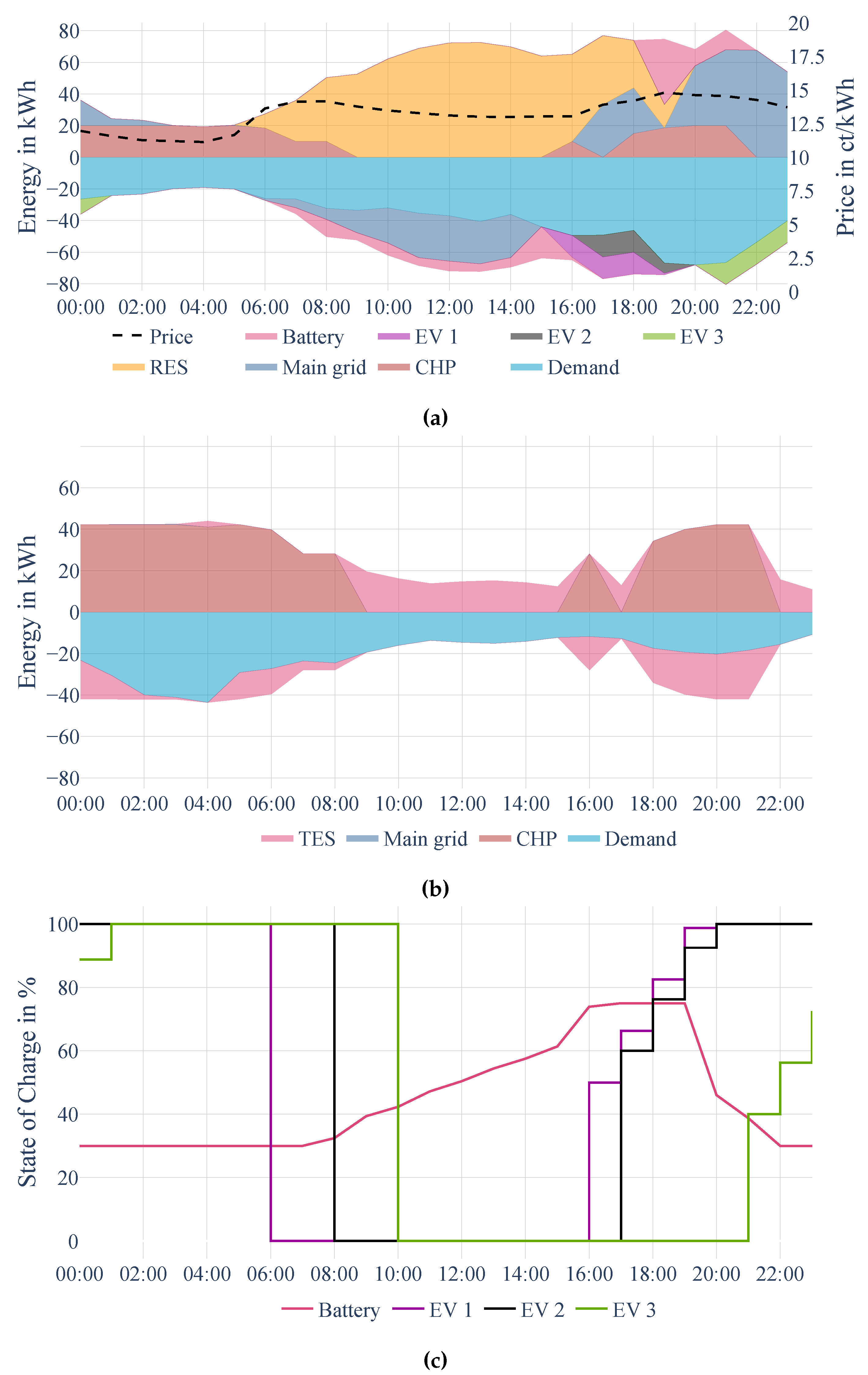
Figure 3.
Smart charging results – Deterministic. (a) Hourly mass balance electricity. (b) Battery and EV SOC profiles.
Figure 3.
Smart charging results – Deterministic. (a) Hourly mass balance electricity. (b) Battery and EV SOC profiles.
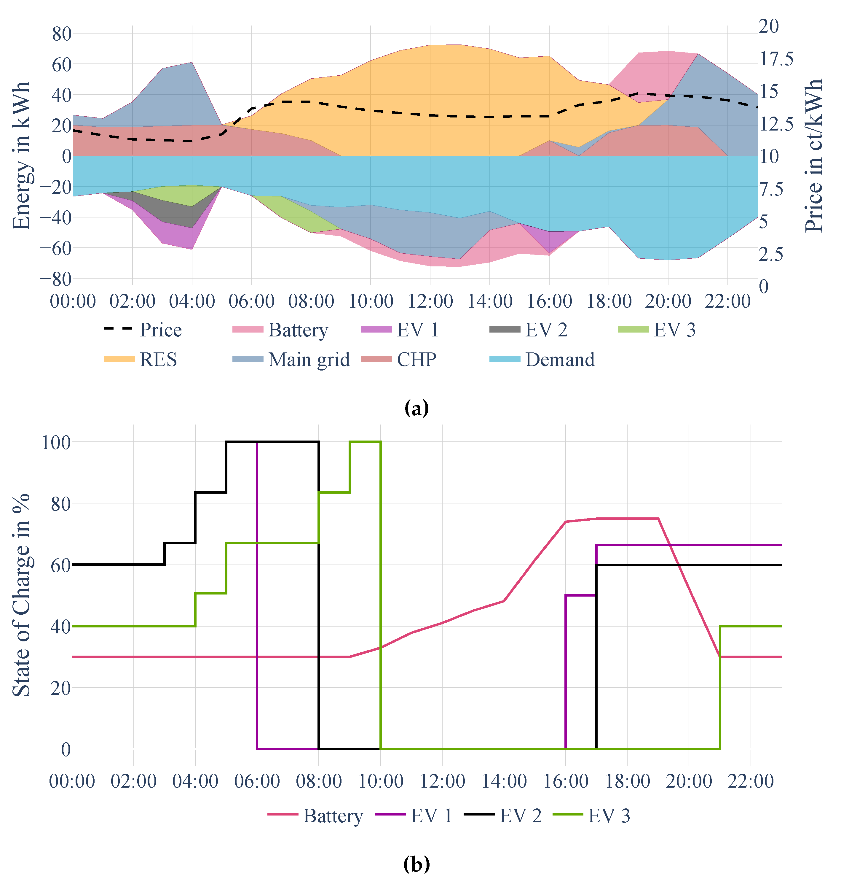
Figure 4.
V2G charging results – Deterministic. (a) Hourly mass balance electricity. (b) Hourly mass balance heat. (c) Battery and EV SOC profiles.
Figure 4.
V2G charging results – Deterministic. (a) Hourly mass balance electricity. (b) Hourly mass balance heat. (c) Battery and EV SOC profiles.
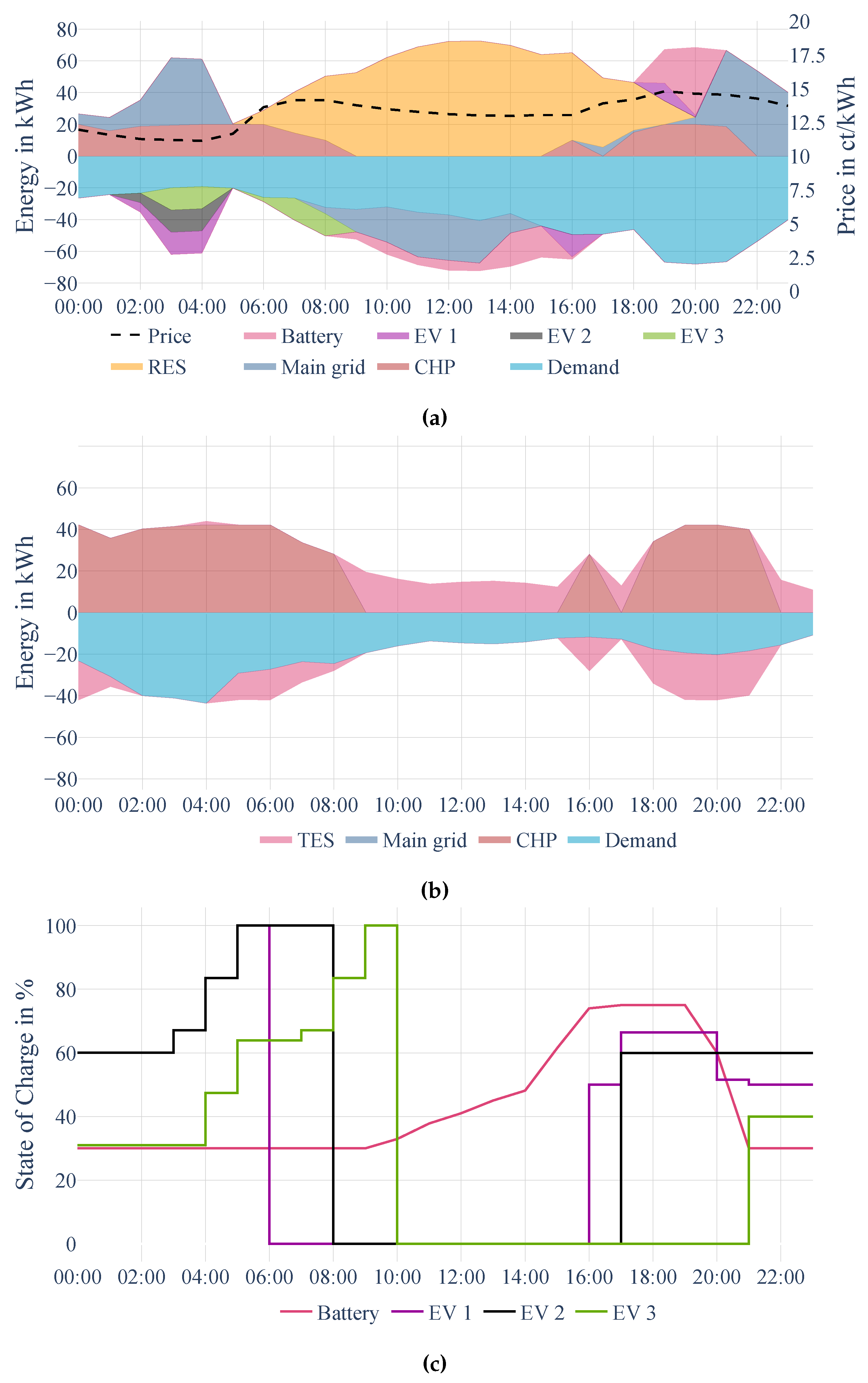
Figure 5.
Price scenarios in the stochastic analysis.
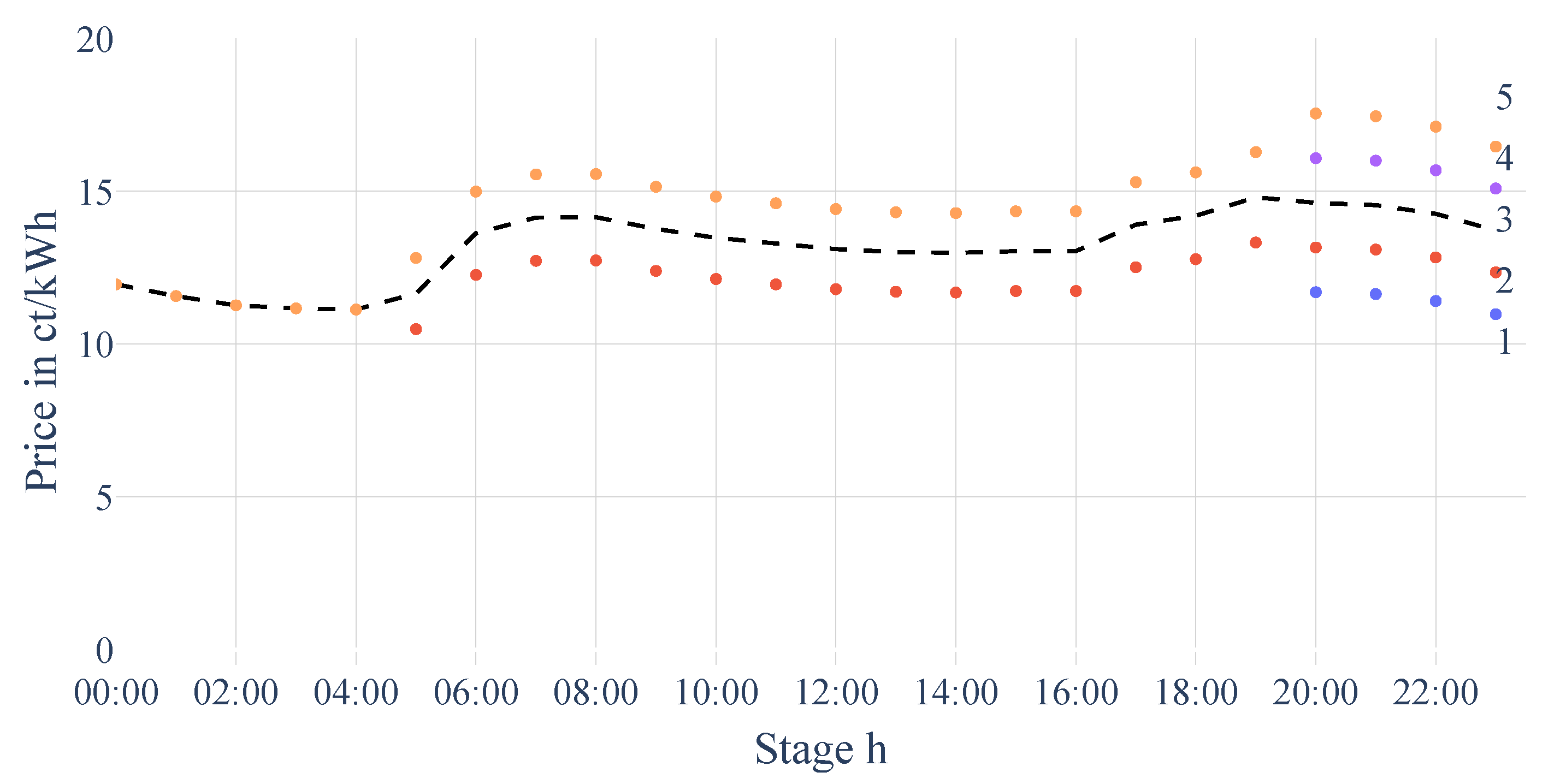
Figure 6.
Scenario tree showing 15 scenarios based on price and EVs’ SOC uncertainties over 24 hours.
Figure 6.
Scenario tree showing 15 scenarios based on price and EVs’ SOC uncertainties over 24 hours.
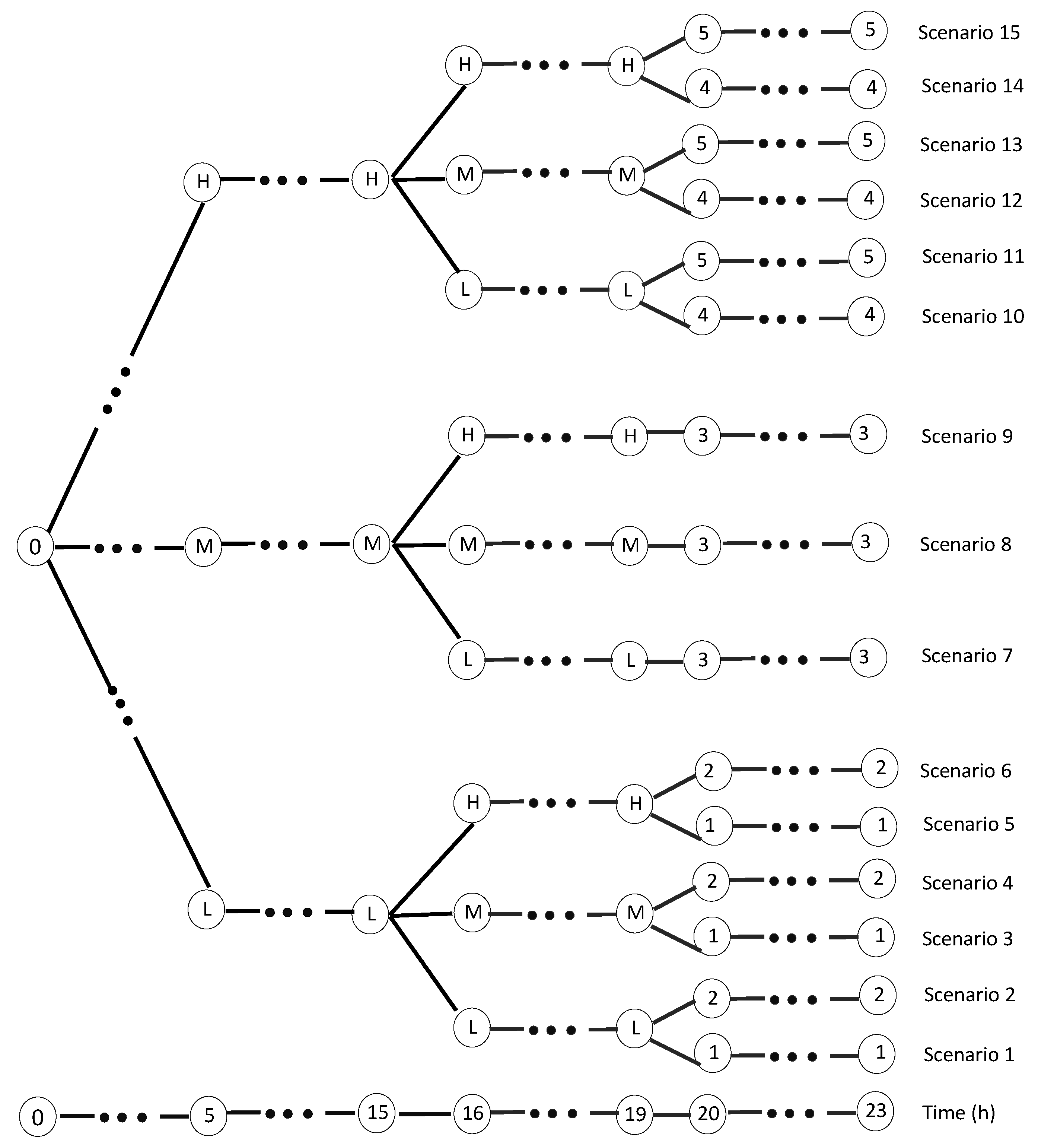
Figure 7.
SOC profiles, Stationary battery, Smart charging, Stochastic. Vertical axis truncated for readability.
Figure 7.
SOC profiles, Stationary battery, Smart charging, Stochastic. Vertical axis truncated for readability.
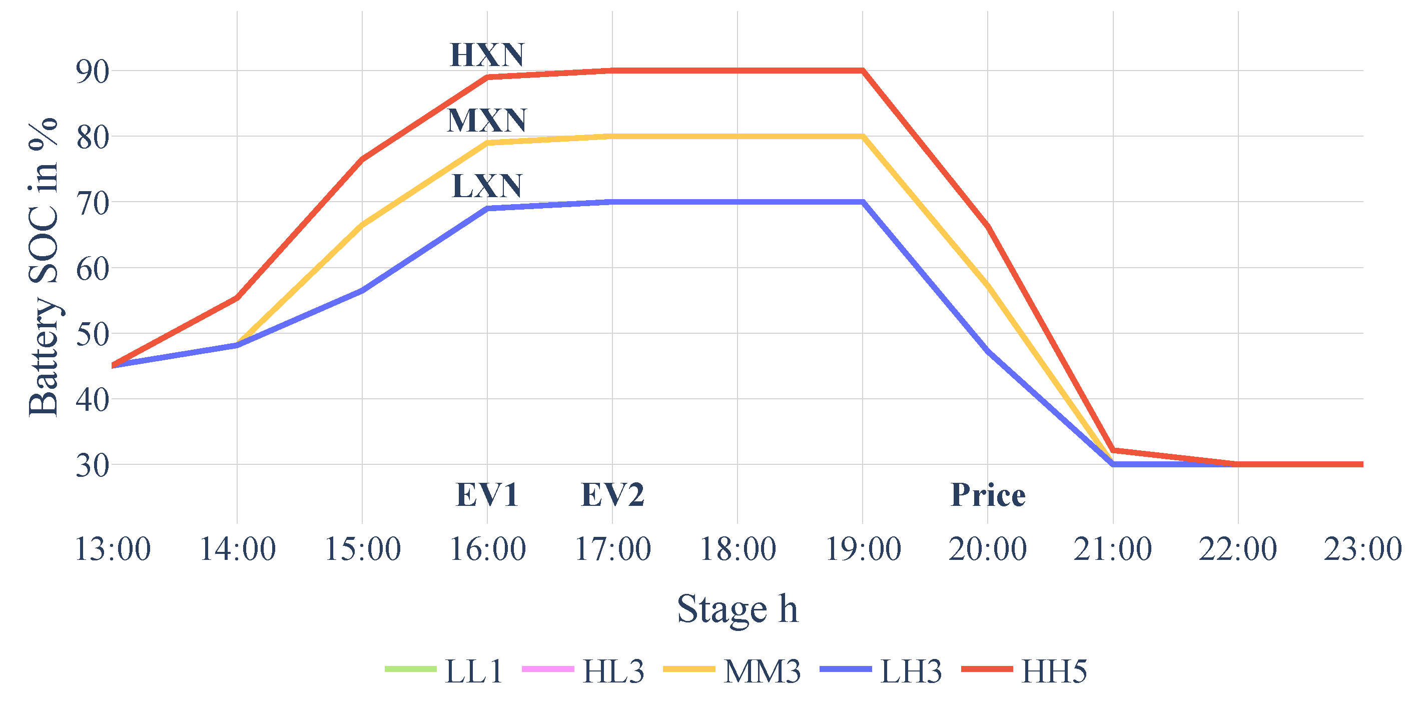
Figure 8.
SOC profiles, EV1, Smart charging, Stochastic.
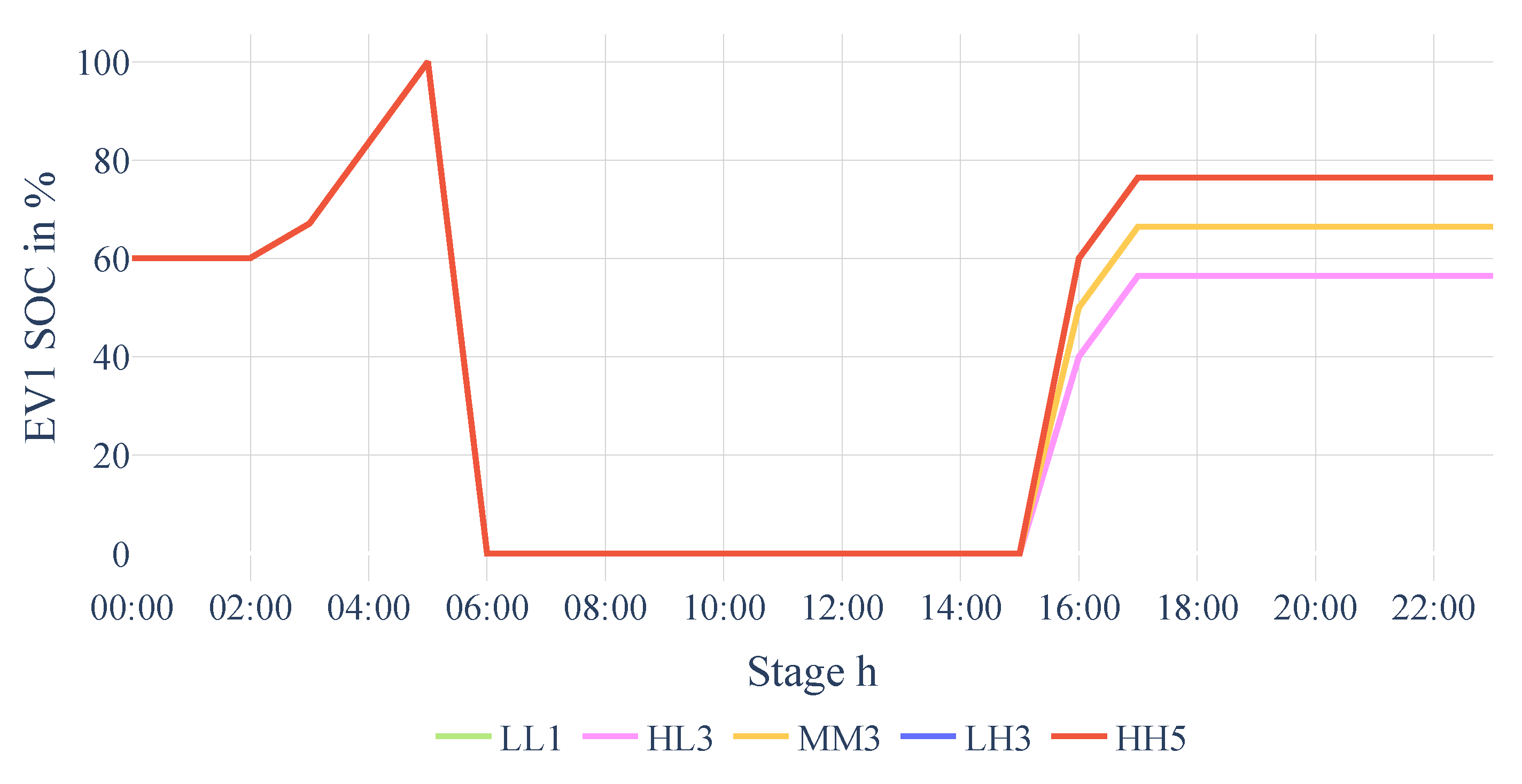
Figure 9.
SOC profiles, EV1, V2G charging—Stochastic. Both axes truncated for readability. Results are shown for all 15 scenarios. For brevity, the legend is only provided for scenarios discussed in the text.
Figure 9.
SOC profiles, EV1, V2G charging—Stochastic. Both axes truncated for readability. Results are shown for all 15 scenarios. For brevity, the legend is only provided for scenarios discussed in the text.
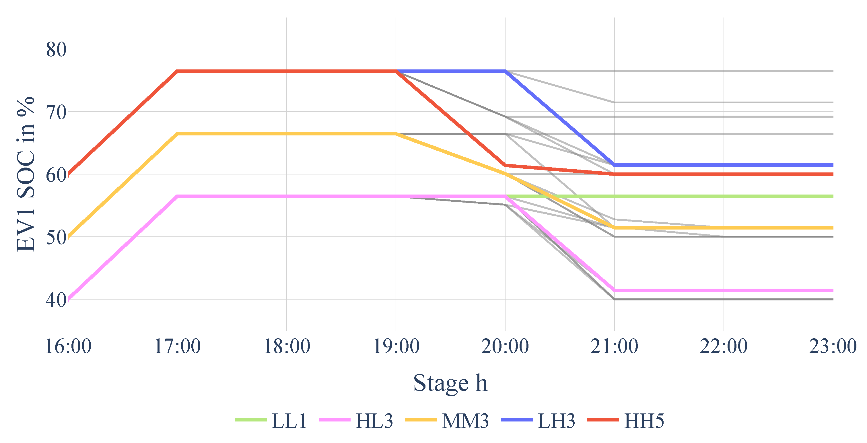
Figure 10.
EV2, V2G charging—Stochastic. Both axes truncated for readability.
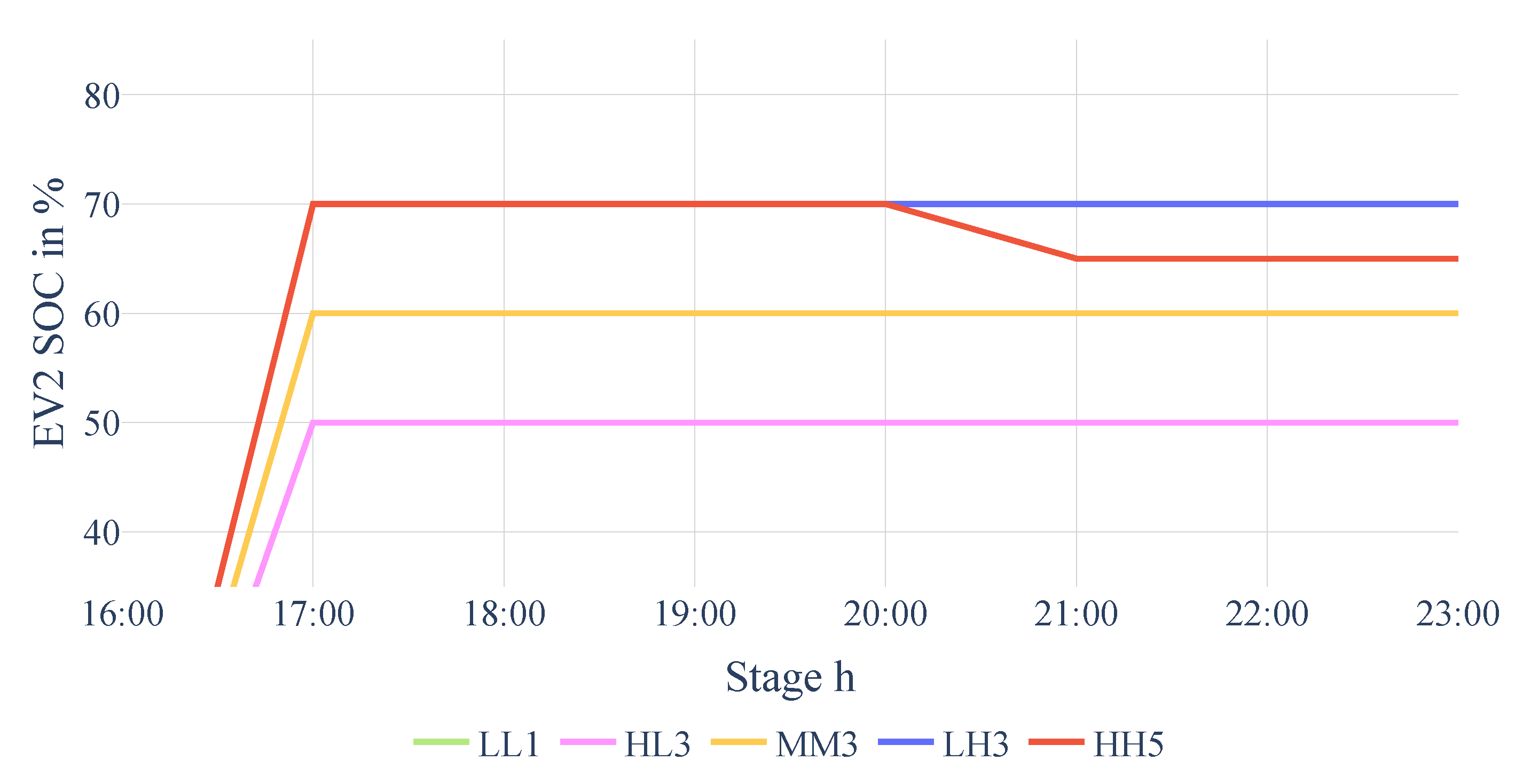
Figure 11.
System cost breakdown. Each column group: left: Passive, middle: Smart, right: V2G. Net grid import costs main grid (-feedin) is the difference between power purchase cost and remuneration for solar power feed-in. Vertical axis truncated for readability.
Figure 11.
System cost breakdown. Each column group: left: Passive, middle: Smart, right: V2G. Net grid import costs main grid (-feedin) is the difference between power purchase cost and remuneration for solar power feed-in. Vertical axis truncated for readability.

Table 1.
CHP segment breakpoint data.
| Operating Level | 0% | 50% | 75% | 100% |
|---|---|---|---|---|
| Gas consumption [kW] | 0 | 37.1 | 48.1 | 61.1 |
| Electric output [kW] | 0 | 10.0 | 15.0 | 20.0 |
| Heat output [kW] | 0 | 28.1 | 34.2 | 42.2 |
Table 2.
Storage characteristics.
| Storage type | Battery | TES | EV (each) |
|---|---|---|---|
| Capacity [kWh] | 150 | 172 | 40 |
| Power [kW] | 90 | 42.2 | 7.0 |
| Round trip efficiency [%] | 90 | 90 | 88 |
| Assumed operating temperature [°C] | 25 | – | 25 |
| Max. capacity loss [%/cycle] | 0.04519 | – | 0.04519 |
| Fatigue strength exponent | 0.4926 | – | 0.4926 |
| Fitting parameter SOC stress[%/cycle] | 0.0085 | – | 0.0085 |
Table 3.
Battery degradation segment breakpoint data .
| Breakpoint | 0% | 30% | 60% | 70% | 100% |
|---|---|---|---|---|---|
| Aging val OLD | 15.01 | 35.02 | 40.02 | 73.62 | 89.34 |
| Aging value y | 3.75 | 8.76 | 10.01 | 18.41 | 22.34 |
Table 4.
Deterministic case KPI.
| KPI | Passive | Smart | V2G |
|---|---|---|---|
| Objective value [€] | 86.45 | 80.16 | 80.13 |
| Battery throughput [kWh] | 64.12 | 64.12 | 64.12 |
| PV generation [kWh] | 681.13 | 681.13 | 681.13 |
| Electric CHP generation [kWh] | 241.31 | 242.50 | 242.50 |
| Peak demand [kW] | 80.46 | 68.08 | 68.08 |
| Peak grid import [kW] | 67.64 | 53.81 | 53.81 |
| Total grid import [kWh] | 294.01 | 273.42 | 268.82 |
| Total grid export [kWh] | 161.08 | 136.34 | 136.34 |
| Annualized stationary battery aging [%] | 4.12 | 4.11 | 4.11 |
| EV battery aging while connected [%]1 | 1.17 | 0.83 | 1.02 |
1 Average annualized EV battery aging while EVs are connected. We ignore degradation from discharges while driving.
Disclaimer/Publisher’s Note: The statements, opinions and data contained in all publications are solely those of the individual author(s) and contributor(s) and not of MDPI and/or the editor(s). MDPI and/or the editor(s) disclaim responsibility for any injury to people or property resulting from any ideas, methods, instructions or products referred to in the content. |
© 2024 by the authors. Licensee MDPI, Basel, Switzerland. This article is an open access article distributed under the terms and conditions of the Creative Commons Attribution (CC BY) license (http://creativecommons.org/licenses/by/4.0/).
Copyright: This open access article is published under a Creative Commons CC BY 4.0 license, which permit the free download, distribution, and reuse, provided that the author and preprint are cited in any reuse.


