Submitted:
14 July 2025
Posted:
15 July 2025
You are already at the latest version
Abstract
The core value of carbon price forecasting lies in reducing uncertainty in carbon markets and promoting the transition to a low-carbon economy. Although significant progress has been made in current carbon price forecasting models, challenges remain in the adaptability of second decomposition algorithms, the depth extraction capability of error correction algorithms, and the handling of non-normality and heteroscedasticity in carbon price data through interval algorithms. To address these issues, this paper proposes a four-stage carbon price forecasting model. First, a second decomposition is performed using ICEEMDAN-VMD optimized by the Difference Innovation Search Algorithm (DCS) and the Central Frequency Method. Next, the TCN-Transformer is used to model the decomposed components separately, with their linear summation providing the preliminary forecast. Then, an improved second decomposition algorithm (ISD) and LSTM are applied to build a deep error correction model, aiming to extract the predictable components from the preliminary forecast errors. Finally, a Bivariate Kernel Density Estimation (BKDE) is constructed using the forecast values and error values from the training set to generate interval prediction results. Case studies from Hubei and Guangzhou demonstrate that the model achieves an R² greater than 0.99 and a PICP greater than 0.95, significantly outperforming existing methods and effectively supporting the implementation of the dual-carbon strategy.
Keywords:
difference innovation search algorithm
; ICEEMDAN
; VMD
; deep error correction
; bivariate kernel density estimation
; carbon price prediction
1. Introduction
In recent decades, the surging global energy demand and excessive exploitation of fossil fuels have led to a sharp increase in atmospheric CO2 concentrations, resulting in record-breaking global temperatures and continuous polar ice melt [1]. This critical situation poses significant challenges to sustainable social development and has driven international consensus on emission reduction targets. As a crucial market-based mitigation instrument, carbon trading markets effectively guide emission control through pricing mechanisms, thereby alleviating the greenhouse effect. In this context, accurate carbon price prediction plays a pivotal role in market optimization[2]. In order to achieve effective prediction of carbon price, scholars have proposed many methods, which can be broadly classified into three categories: traditional statistical models, machine learning models and hybrid models.
Traditional statistical models predict carbon prices by analyzing historical trend and cyclical components, with typical examples being ARIMA and GARCH models. For instance, García [3] developed a vector ARIMA model that successfully achieved point value forecasting for carbon prices. Byun [4] demonstrated the superiority of GARCH-type models over KNN algorithms in predicting EU carbon allowance prices. Although statistical models can effectively capture linear patterns in historical data, their inherent linear assumptions fundamentally conflict with the pronounced nonlinear characteristics and chaotic nature of carbon price data [5], making it difficult to meet practical requirements for prediction accuracy.
With technological advancements, machine learning models have emerged as pivotal tools for carbon price prediction due to their exceptional nonlinear learning capabilities [6]. Early-stage research primarily employed shallow neural networks, including BPNN[7], ELM[8], and MLP. Notable studies include: Li [9] developed a genetic algorithm-optimized ELM for Beijing carbon market price forecasting; Wang [10] established a BPNN-based prediction model; while Fan [11] enhanced prediction accuracy by integrating chaos theory with MLP modeling.
Recent years have witnessed deep learning algorithms becoming mainstream owing to their superior nonlinear learning and temporal modeling capacities. Huang [12] innovatively proposed an OHLC data transformation method coupled with CNN; Pan [13] incorporated unstructured factors like investor attention into LSTM modeling; and Yun [14] developed a NAGARCHSK-GRU hybrid framework to capture higher-order moment characteristics of carbon prices.
While machine learning models effectively address the limitations of statistical models in capturing nonlinear relationships and significantly improve prediction performance, their effectiveness largely depends on the quality of the input data. The high volatility of carbon price data often leads to overfitting in single machine learning models, resulting in unstable predictions [15]. Therefore, researchers have introduced decomposition algorithms to enhance model prediction performance.
Decomposition algorithms, by breaking down the complex fluctuations in carbon price data into simpler components, not only improve the quality of the input data but also reduce the impact of noise on the model. In earlier studies, scholars primarily used methods such as EMD [16], EEMD [17], and CEEMD [18]. However, EMD, EEMD, and CEEMD have limitations in mode mixing and decomposition accuracy. As a result, researchers began to introduce various improved decomposition algorithms to decompose data. Commonly used improved decomposition algorithms include CEEMDAN, ICEEMDAN, and VMD. For instance, Wang [19] demonstrated the effectiveness of CEEMDAN in filtering irrelevant features; Huang [20] used VMD for data decomposition and compared it with the EMD method, showing that VMD significantly outperforms EMD; Zhou [21] compared ICEEMDAN, CEEMDAN, and EEMD, finding that ICEEMDAN performed notably better than the other two methods. However, many studies suggest that predicting high-frequency components after a single decomposition remains challenging [22]. To address the difficulty of predicting high-frequency components, cutting-edge research has adopted secondary decomposition techniques. Cheng [23] proposed the VMD-RE-ICEEMDAN method, which demonstrates significant advantages over traditional methods.Lan [24] proposed the IVMD-ICEEMDAN-SOA integrated model, which not only resolves the parameter optimization issue of VMD through algorithmic improvements but also enhances the model’s generalization ability through its hierarchical prediction framework, taking the model’s performance to a new level.
Although the secondary decomposition algorithm significantly improves forecasting accuracy, most existing secondary decomposition algorithms focus primarily on optimizing the parameters of VMD, with limited research on optimizing the parameters of other decomposition algorithms. This results in suboptimal decomposition accuracy and insufficient adaptability in secondary decomposition.
Moreover, related studies indicate that there are still many predictable components hidden within the prediction errors. To effectively extract useful components from the errors, researchers have gradually started using error correction algorithms to refine the initial predictions, leading to a significant leap in forecasting accuracy. For instance, Hu [25] improved the performance of the model by using SSA-MKELM to correct prediction errors based on the VMD-TVFEMD-SSA-MKELM framework. Similarly,Yang [26]employed ELM to correct the preliminary results in secondary decomposition ensemble forecasting, effectively reducing prediction errors. These studies demonstrate that the application of error correction algorithms can significantly improve model performance and reliability. However, they do not account for the fact that predictable components at different frequencies still exist within the error sequence, making the error correction effect weaker. As a result, many scholars have begun combining decomposition algorithms with error correction algorithms to effectively extract different frequency components within the error sequence. For example, Li [27]used EEMD to decompose the errors into multiple IMFs, then used LSTM and ELM to predict high-frequency and low-frequency IMFs separately. Xu [28]utilized VMD-KELM to build an error correction algorithm for this purpose. These findings show that combining decomposition algorithms with error correction modules can significantly enhance forecasting accuracy and reliability.
However, these error correction algorithms typically apply single decomposition algorithms to handle the error sequence. Numerous studies have shown that the decomposition accuracy and stability of single decomposition algorithms are lower than those of secondary decomposition. Additionally, the complexity of the error sequence can be comparable to or even greater than that of the original sequence. Therefore, existing error correction algorithms lack research that integrates secondary decomposition algorithms, leading to insufficient deep extraction capabilities for the predictable components in the error sequence.
Besides, the above models are all point forecast models, but the single point forecast result cannot effectively measure the risk of carbon price fluctuation. Therefore, scholars have started to focus on interval forecasting, which, unlike point forecasting, can provide the boundary value of carbon price fluctuation and provide more references for related practitioners. Common interval estimation algorithms such as KDE[29], Bootstrap[30] and GPR[19]. For example: Ji [31] first decomposes the raw carbon price data using ICEEMD, after that constructs the SSA-BPNN point prediction estimation model, and finally constructs the carbon price intervals using KDE based on the point prediction. Zeng[32] uses enhanced KDE to construct carbon price intervals. However, the KDE、Bootstrap and GPR et al. algorithm ignores the heteroskedasticity of the carbon price data, so the existing carbon price interval estimation is in urgent need of a model that can describe the non-normality and heteroskedasticity of the carbon price data at the same time. To address these shortcomings, In this paper, a hybrid model based on depth error correction and binary kernel density estimation (BKDE) is proposed, which firstly uses DCS-ICESEMDAN-OVMD to quadratically decompose the original carbon price data to obtain multiple components with different frequencies; then, a TCN-Transformer prediction model is constructed for each component to obtain the preliminary prediction results; after that, an improved quadratic decomposition combined with LSTM is constructed to correct the preliminary prediction results. Then, the TCN-Transformer prediction model is constructed for each component, and the preliminary prediction results are obtained; after that, the improved quadratic decomposition and LSTM are combined to construct a deep error correction algorithm to correct the preliminary prediction results; finally, the point prediction results and the error values of the training set are inputted into the BKDE, and the distribution relationship between the point prediction values and the error values is obtained, so as to obtain the upper and lower bounds of the intervals according to the point prediction results of different test sets. The main innovations are as follows:
(1) In this paper, the parameters of ICEEMDAN and VMD are optimised using the DCS method and the centre frequency method, respectively, which not only improve the adaptive ability of the quadratic decomposition algorithm, but also improve the decomposition accuracy of the quadratic decomposition algorithm, and achieve more refined modelling.
(2) The deep error correction algorithm is proposed for the first time in the field of carbon price forecasting, combining the improved quadratic decomposition algorithm with deep learning. This approach effectively extracts the different frequency components in the error sequence, significantly enhancing the error correction capability of the algorithm.
(3) Propose a bivariate kernel density estimation algorithm to construct carbon price intervals to make up for the fact that the current carbon price interval prediction model does not adequately take into account the non-normality and heteroskedasticity of carbon price data.
The structure of the article is as follows: Chapter 2 outlines the methodology employed for the hybrid model presented in this paper. Chapter 3 details the specific process of the proposed hybrid model. Chapter 4 presents experimental results from the Hubei and Guangdong carbon markets, elaborating on each module of the model and conducting four control experiments to validate the effectiveness of the proposed method. The final section concludes with a summary of the key findings and offers an outlook for future research.
2. Materials and Methods
2.1. ICEEMDAN Based on DCS Optimisation
2.1.1. ICEEMDAN
The ICEEMDAN algorithm is an algorithm derived from CEEMD. It defines the residuals of the previous period obtained by iterative computation minus the residuals of the current period as the IMF formed by each iteration. Compared with CEEMD, this algorithm is more effective in suppressing the modal aliasing phenomenon in the decomposition process.[33]. The specific process is shown as follows:
(1) Add Gaussian white noise with mean 0 and variance 1 to the original signal.
(2) The local mean of the constructed signal is averaged to obtain the residuals and the first modal component.
(3) Estimate the second residual and the second modal component using the local mean of the second signal.
(4) And so on until the residuals cannot be further decomposed.
2.1.2. DCS-Based Optimisation of ICEEMDAN Parameters
Differentiated Creative Search (DCS) algorithm, different from traditional optimisation algorithms, revolutionises the traditional decision-making system in complex environments by simulating creative divergence and convergence behaviours, flat horizontal global search and local optimisation. Its core idea is to generate diversified solutions through randomisation or heuristic methods to simulate human’s divergent thinking in problem solving, and through this creativity-generating mechanism, the DCS algorithm can explore widely in the search space to avoid falling into local optimality; secondly, in the generated solutions, it simulates the process of human’s choosing the optimal solution among the many creative ideas by evaluating the fitness of the solutions and selecting the ones that are significantly differentiated, and the This differential selection mechanism enables the algorithm to dynamically adjust the search strategy according to the problem characteristics[34].Therefore, the DCS algorithm is suitable for a wide range of complex optimisation problems.
Although ICEEMDAN can solve the modal aliasing problem of EMD and EEMD by adding different degrees of white noise at each iteration, it has been a problem to determine the number of times ICEEMDAN adds noise and the intensity of the added noise. Relevant studies have shown that too many noise additions can lead to noise residuals after ICEEMDAN decomposition, which affects the accuracy of decomposition, and too few noise additions can lead to modal aliasing in ICEEMDAN; at the same time, too high a noise intensity can mask the real signal, which leads to distortion of the decomposition results, and too low a noise intensity can also trigger the effect of modal aliasing. Therefore, choosing the appropriate number of noise additions and noise intensity is conducive to improving the decomposition effect of ICEEMDAN. In this paper, DCS is used to optimise the key parameters of ICEEMDAN to improve the adaptive ability and decomposition effect of ICEEMDAN. The specific algorithm flow is shown below:
(1) Initialisation: assume that the population size is N and each individualis a D-dimensional vector representing a set of ICEEMDAN parameters. The initialisation formula is shown in Equation 1:
where represents the JTH dimension component of the i-th individual, and are respectively the upper and lower bounds of the search space of the j-th dimension, is random numbers within the interval [0,1]. In this paper, the search interval for the number of noise additions is set as [0,500], and the noise amplitude is set as [0,1].
(2) Idea generation: generating new solutions by methods such as random perturbation or checkpointing variants. The generation formulas for random perturbation and check score variation are represented by Equation (2) and Equation (3), respectively.
where is the disturbance intensity parameter, is a standard normally distributed random number; ,, are three different individuals randomly selected from the population, and F is the checkpointing variance factor, which is used to control the intensity of the variance.
(3) Adaptation evaluation: calculate the minimum sample entropy of each solution and evaluate its advantages and disadvantages. The adaptation degree calculation formula is shown in Equation 4:
(4) Differential selection: selecting some solutions into the next generation population based on fitness values and differential strategies. The selection formula is shown in Equation (5):
where is the newly generated solution and is the current solution.
(5) Iterative updating: the process of idea generation, evaluation and selection is repeated until the termination conditions are met. The update formula is shown in Equation (6):
where is the new generation of populations.
2.2. OVMD
2.2.1. VMD
The VMD algorithm is a classical decomposition algorithm with strict mathematical derivation, and its decomposition efficiency and robustness are significantly better than the CEEMD algorithm[35]. Mathematically, the VMD decomposition process is formulated as Equation (1):
where is the K-th component of the decomposition and is the centre frequency of the K-th component.However, Equation (7) cannot be solved directly, so K. Dragomiretskiy and D. Zosso introduced the quadratic penalty function and Lagrange multipliers to convert Equation (7) into a problem of finding the extreme value, as shown in Equation (8).
Finally, Equation (8) is solved by the alternating multiplier method; the optimal solution of Equation (7) is obtained by constantly updating, , and solving the “saddle point” of the improved Lagrangian expression. The new modal components of the solution and the calculation of the centre frequency are shown in Equations (9) and (10), respectively:
2.2.2. OVMD Based on Centre Frequency
Although the Variational Mode Decomposition (VMD) algorithm demonstrates superior decomposition accuracy and robustness compared to EMD、EEMD and CEEMD, its performance critically depends on the selection of the key parameter K (the number of intrinsic mode functions). An insufficient K-value may result in incomplete decomposition, causing mode mixing across different frequency components. Conversely, an excessively large K-value can induce over-decomposition, producing redundant modes that degrade subsequent prediction performance and increase computational overhead[36]. To address this limitation, we propose an optimized VMD (OVMD) algorithm, which automatically determines the optimal K-value based on center frequency analysis.
According to the VMD principle, each decomposed mode is characterized by a distinct center frequency. By iteratively increasing K, we can evaluate the significance of newly generated modes by monitoring their center frequency convergence. Specifically:
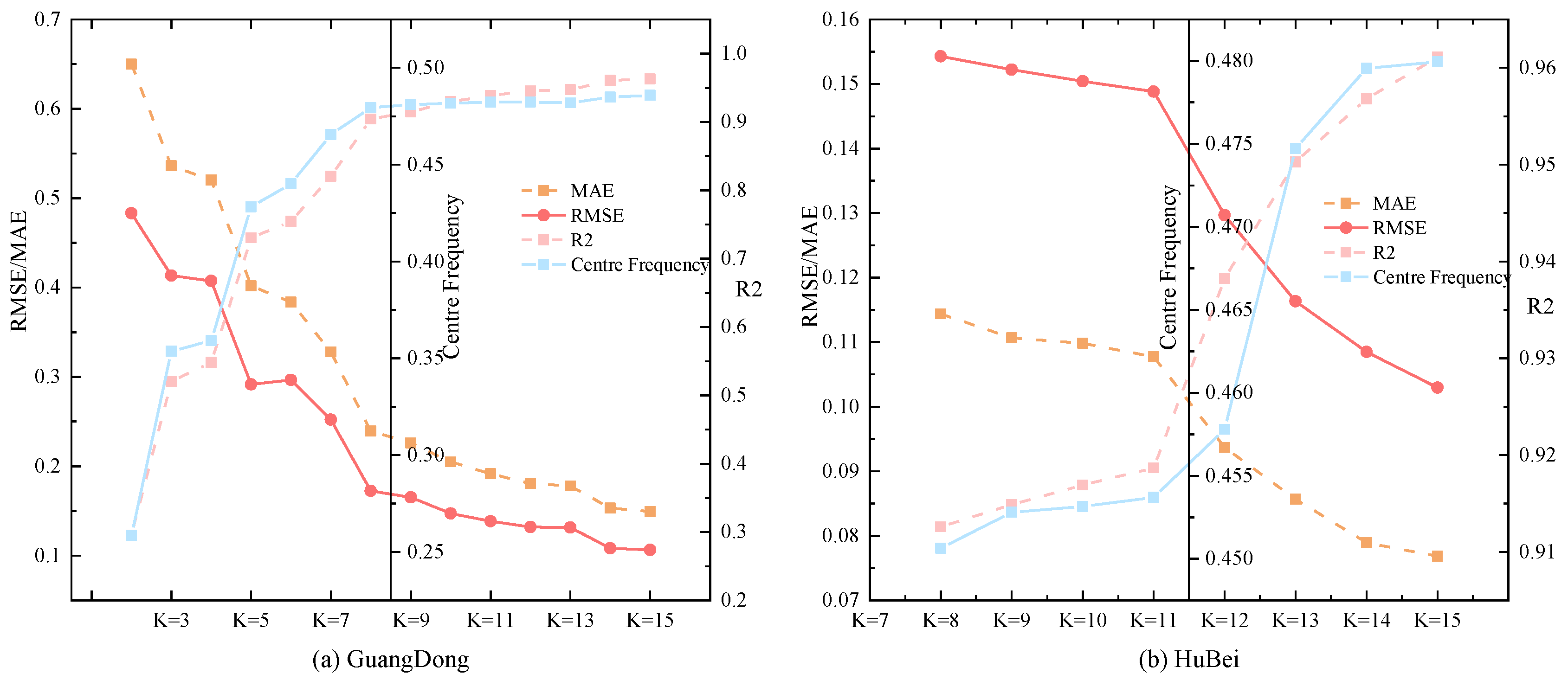
If the center frequency of a new mode closely matches that of a previous iteration, the component is deemed redundant and contributes minimally to meaningful signal decomposition. Conversely, significant fluctuations in center frequency indicate the emergence of physically relevant modes. To illustrate this, Figure 5 plots the center frequency variation versus K. Key observations include:
Initial increases in K yield substantial center frequency shifts, reflecting the extraction of meaningful signal components. Beyond a critical K-value (K = 9 in our case), the center frequencies stabilize, indicating diminishing returns in mode separation. As shown in Figure 5a, the error metrics (RMSE, MAE, MAPE, R2) concurrently stabilize at K = 9, confirming this value as the optimal trade-off between decomposition fidelity and computational efficiency. This inflection point in center frequency behavior allows us to objectively select the optimal K, ensuring efficient and accurate time-series decomposition without manual tuning.
2.3. Deep Learning Algorithm
2.3.1. TCN-Transformer
The TCN-Transformer model integrates Temporal Convolutional Networks (TCNs) and the Transformer architecture to capture short-term non-linear trends and long-term contextual dependencies in carbon price dynamics. The design addresses key challenges in carbon market forecasting: high volatility and complex macroeconomic implications.
(1) TCN is a neural network architecture designed using inflated causal convolution, and its most central structures include causal convolution, inflated convolution, and residual connection structures[37]. The specific calculations of the three structures are shown below. In the case of a one-dimensional time series, the calculation of causal convolution is expressed as:
where is the t-th element of the output sequence, is the t-m+1st element of the input sequence, is the m-th weight of the convolution kernel, and k is the size of the convolution kernel.
Expansion convolution expands the sensory field of the convolution kernel by introducing spacing in the convolution kernel without increasing the size of the convolution kernel. Given an input sequence x, a convolution kernel of size k ω editor output and an expansion rate d, the computation of the expansion convolution is denoted as:
where is the rate of expansion.
A residual module contains two inflated causal convolutional layers, with WeightNorm and Dropout added to each layer to regularise the network, and a 1*1 convolution added to keep the input and output scales the same. The exact calculation is shown below:
where and are the output inputs, respectively, and is the nonlinear transformation of the residual block.
(2) Transformer is a deep learning architecture based on Self-Attention, whose core modules include: multi-head attention mechanism, positional coding, residual linking and layer normalisation and feed-forward neural network[38]. Compared with RNN/CNN, Transformer can directly model global dependencies, which is suitable for tasks such as carbon price prediction that need to balance local fluctuations and macro trends. The formulae for each module are shown below:
Equation 14 shows the calculation method of positional coding, where represents the input data, represents the embedding matrix, and represents the sine/cosine coding.
Equation 16 shows the calculation method of the multi-attention mechanism, where are the three attention weights and is the query dimensions, respectively.
Equation 17 shows the feed-forward neural network calculation method, where are the weight value and are the deviation value.
where is self-attention and is layer normalisation.
(3)The TCN-Transformer architecture in this paper combines the local temporal extraction of TCN, and the global dependency modelling of Transformer to construct a complementary two-stage feature processing flow. The architecture first employs stacked inflated causal convolutional layers of the TCN module to capture local patterns and multi-scale dependencies of time series hierarchically while strictly maintaining temporal causality; then Transformer is used to establish global temporal dependencies through a self-attention mechanism to identify long-range patterns of carbon valence sequences across time steps[39].
2.3.2. LSTM
The Long Short-Term Memory (LSTM) network, proposed by Sepp Hochreiter and Jürgen Schmidhuber in 1997, introduced a novel approach to recurrent neural networks. Unlike traditional RNNs, LSTM incorporates memory cells and gating mechanisms, effectively addressing the issues of vanishing and exploding gradients in RNNs when processing long-term time series data. This advancement significantly enhances the ability to capture long-term dependencies and has since been widely applied in various time series prediction tasks, such as wind speed forecasting, pollutant prediction, carbon price forecasting, and load forecasting.
2.4. Bivariate Kernel Density Estimation
Bivariate Kernel Density Estimation (BKDE) is a nonparametric statistical technique for estimating the joint probability density function (PDF) of a two-dimensional random variable. Unlike conventional univariate kernel density estimation (KDE), BKDE extends the kernel smoothing approach to 2D space by centering a symmetric kernel function at each observed data point and aggregating their contributions to construct a smooth density surface. This enables BKDE to capture the interdependency between two variables, such as the relationship between prediction errors and associated covariates, while automatically adapting to heteroskedasticity—a key limitation of standard KDE[40]. The general equations of the BKDE are shown below for a given bivariate dataset X1,X2:
where K is a kernel-nonnegative function and h is known as the bandwidth parameter. The kernel function K must satisfy the non-negativity condition to ensure valid probability density estimates. The bandwidth parameter h plays a crucial role in determining the estimator’s performance - it controls the trade-off between bias and variance in the density estimation. An optimal bandwidth selection yields confidence intervals with both higher coverage probability and narrower width, while suboptimal choices may lead to either oversmoothing or undersmoothing.
To achieve optimal bandwidth selection, we employ the Mean Integrated Squared Error (MISE) criterion, which provides a balanced measure of estimation accuracy by considering both bias and variance. The MISE is defined as:
3. The Proposed Model
In this study, a new decomposition integral model is proposed for predicting interval-valued carbon prices. The model integrates improved quadratic decomposition, deep learning and bivariate kernel density estimation methods. As shown in Figure 1, the proposed framework contains five different steps.
3.1. Data Collection
The first step is to collect the historical data of the closing carbon price and its related financial products, and fill in the missing values using the linear difference method to finally obtain the historical data of the carbon price.
3.2. Improved Secondary Decomposition
The second step involves breaking down the complex carbon valence sequence into simpler subsequences using an enhanced quadratic decomposition approach. Initially, the ICEEMDAN parameters are optimized using the DCS algorithm to perform a primary decomposition, extracting the fundamental frequency components of the original carbon price. In the subsequent step, the high-frequency components, which are challenging to predict, are further decomposed using a center-frequency-based variational modal decomposition, also known as the optimal variational modal decomposition, to isolate the potentially predictable components.
3.3. Deep Learning
In the third step, TCN-Transformer is used to model the predictions for each component following quadratic decomposition. Point predictions are generated for each component and then combined through a linear summation to produce the final prediction results.
3.4. Depth Error Correction
In the fourth step, the error sequence is first decomposed quadratically using DCS-ICEEMDAN-OVMD, and then the components are modelled and predicted using LSTM, and the error prediction results are obtained by linear integration.
3.5. Interval Forecast
Since the carbon price is not only affected by the long-term trend formed by the supply and demand relationship, but also by the short-term fluctuations generated by a variety of exogenous factors, the results of the point prediction can not achieve 100 % prediction, and the existence of the error value is inevitable. In order to quantify this uncertainty, this study constructs a BKDE model using point forecasts and error values to obtain the final interval forecast results.
3.6. Accuracy Assessment
To comprehensively assess the model’s predictive performance, we employed two categories of evaluation metrics: point prediction accuracy measures (RMSE, MAE, MAPE, R2), and interval prediction quality indicators (PICP, PINAW, CWC). Calculated as shown in equations 20-26, where:andrepresent their actual and predicted values.represents the upper and lower bounds of the interval forecast,,, and are the values of the parameter metrics used to calculate the CWC, which are 0.1, 6, 15, and 0.9, respectively.
4. Experiments and Analysis
In this paper, six groups of controlled experiments are designed with Guangdong and Hubei carbon markets as examples. Experiment 1 compares the four models GRU, TCN, Transformer and TCN-Transformer to verify the superiority of TCN-Transformer; Experiment 2 compares the prediction performance under the no-optimisation algorithm and the PSO, GWO, WAA and DCS algorithms, respectively, to verify the superiority of the DCS algorithm; Experiment 3 compares the four models GRU,TCN, Transformer and TCN-Transformer models under different decomposition algorithms to verify the superiority of ISD; Experiment 4 compares the error correction algorithms under no decomposition, primary decomposition and secondary decomposition, and verifies the superiority of the depth error correction; Experiment 5 selects the three state-of-the-art prediction models, and verifies the point prediction methods proposed in this paper to verify the superiority; Experiment 6 compares the prediction performance of six sets of interval estimation algorithms, namely T location Scale, Logistic, Normal, GMM, KDE and BKDE, and verifies the superiority of BKDE. All the experiments in this paper were conducted five times and the average of the five results was taken, and the software used was MATLAB 2023b.
4.1. Data description
The datasets selected in this paper are Hubei carbon market data from 2020/1/2-2024/5/10 and Guangdong carbon market data from 2020/1/2-2024/5/13, and the statistical descriptions of the two datasets are shown in Table 1. As can be seen from Table 1, the carbon price in the Guangdong carbon market is more volatile and more expensive, and the carbon price in the Hubei carbon market is relatively less volatile. The historical data of the two datasets are shown in Figure 2.
4.2. DCS-ICEEMDAN-OVMD
As shown in Table 1 and Figure 2, the carbon price series exhibits significant volatility and nonlinear characteristics, making direct application of deep learning algorithms often ineffective. To mitigate this volatility and high-frequency noise, this study utilizes the DCS-ICEEMDAN-OVMD method to decompose the carbon price series.
Taking the Guangdong dataset as an example, the decomposition results using DCS-ICEEMDAN are presented in Figure 3. From the figure, it is evident that the decomposition method achieves high accuracy, with the fluctuation frequencies from IMF1 to RES showing a gradual decrease. Moreover, there is no overlap between the dominant frequencies of each IMF, indicating that modal aliasing is not a significant issue. Each component represents a distinct frequency type, demonstrating the effectiveness of the DCS-ICEEMDAN decomposition.
While the DCS-ICEEMDAN decomposition provides good results, predicting the high-frequency components after primary decomposition remains challenging. Previous studies have indicated that secondary decomposition techniques can reduce the prediction difficulty of high-frequency components, leading to significant improvements in prediction accuracy. To address this, the OVMD algorithm is applied to further decompose IMF1, uncovering more predictable components. The results of the OVMD decomposition are shown in Figure 4.
To assess the impact of parameter selection on OVMD, this study compares the prediction accuracy of the TCN-Transformer under different parameters. The results, including error metrics and center frequencies, are displayed in Figure 5. As shown in Figure 5, the model’s prediction performance for high-frequency components improves as the value of K increases. However, the improvement in error metrics starts to show diminishing returns beyond a certain K value, suggesting that further increasing the decomposition layers after this threshold provides little additional benefit.
Thus, this study selects the optimal K value for OVMD decomposition for each monthly dataset, ensuring both prediction accuracy and computational efficiency by avoiding over-decomposition. Based on the trends in center frequencies and error index optimization, 9 decomposition components are chosen for the Guangdong dataset, and 14 components for the Hubei dataset, striking a balance between prediction accuracy and the practical applicability of the model.
Figure 5.
Error metrics and centre frequencies of OVMD at different values of K.
4.3. Deep Learning Prediction Results
Research indicates that deep learning algorithms excel in forecasting interval carbon prices due to their robust ability to model time series and capture both nonlinear and linear dependencies. The TCN-Transformer model integrates the local feature extraction strength of TCN with the global feature recognition power of Transformer, making it more effective for carbon price prediction than using either the TCN or Transformer models alone. The point prediction results are displayed in Figure 6.
4.4. Depth Error Correction Results
As shown in Figure 6, the initial prediction results exhibit significant bias during periods of extreme carbon price fluctuations. This is due to the carbon price being influenced by various exogenous factors, making it challenging to extract all relevant information at once using DCS-ICEEMDAN-OVMD combined with TCN-Transformer. Figure 7 displays the sample entropy values of the prediction errors and the original sequence under four parameters, which indicates that both the error sequence and the original sequence contain many predictable components at different frequencies. To deeply extract the predictable components from the error sequence, this paper first applies an improved quadratic decomposition to break down the error sequence into several smooth components. Then, an LSTM prediction model is established to correct the initial prediction results. The prediction results of the error values are shown in Figure 8. As seen from Figure 8, the deep error correction algorithm proposed in this paper effectively extracts the latent features from the error sequence, achieving a second leap in prediction accuracy.
4.5. Interval Prediction Results
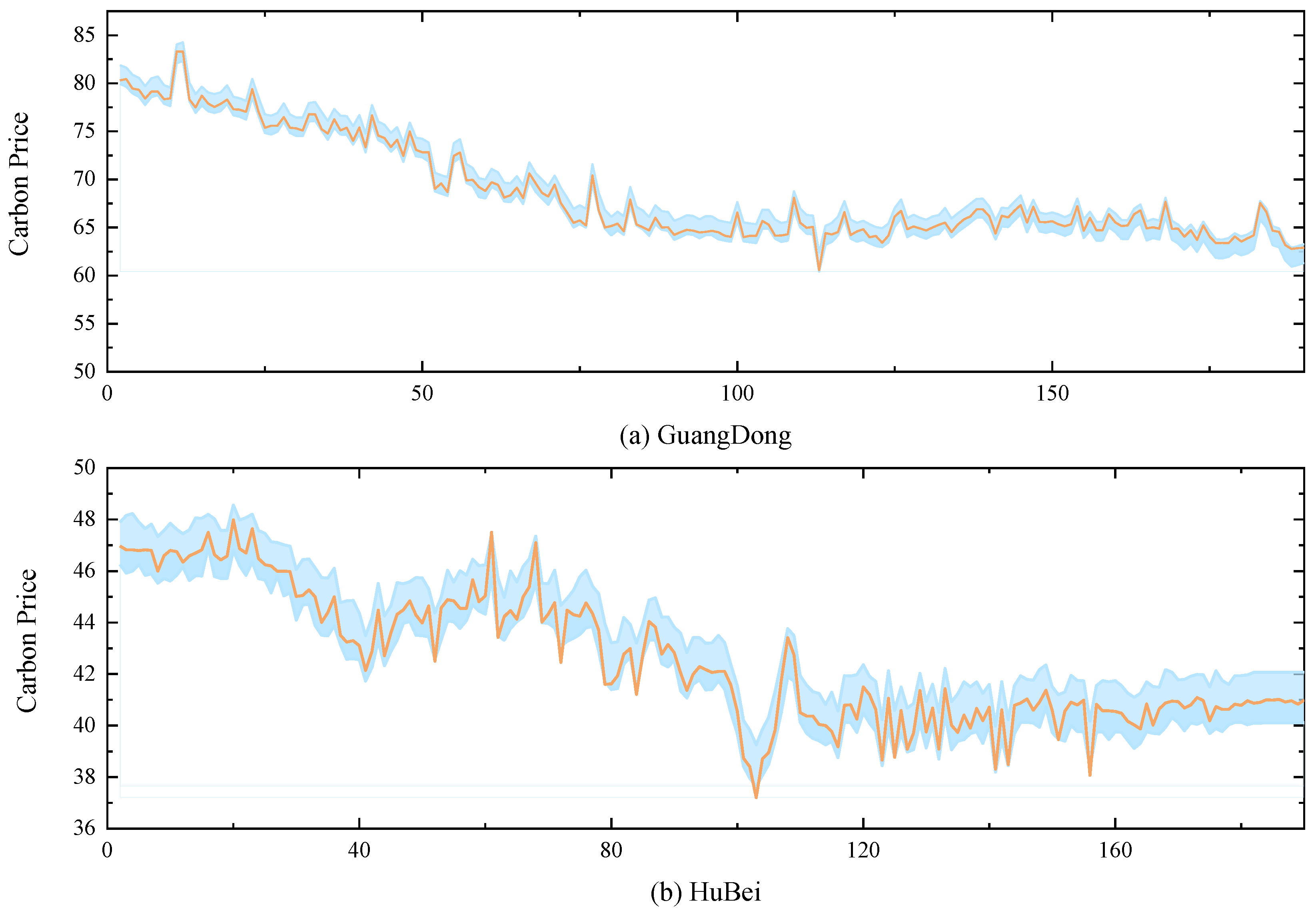
In practice, it is not feasible to account for all factors influencing carbon prices, nor is it possible to include every variable in the model. As a result, prediction errors are inevitable. To offer a more comprehensive understanding of carbon price fluctuations, this study employs bivariate kernel density estimation (BKDE) to capture the uncertainty surrounding carbon prices. This approach effectively addresses the limitations of the existing KDE algorithm, which struggles to account for heteroskedasticity and non-normality in carbon price data. The BKDE prediction results, with 95% confidence intervals, for both datasets are presented in Figure 7. The figure demonstrates that the BKDE interval estimation algorithm proposed here provides broad coverage of actual carbon prices while maintaining an appropriate interval width. Even during sharp fluctuations, the BKDE algorithm ensures high interval coverage, effectively measuring the uncertainty of carbon prices and offering more detailed insights for practitioners.
Figure 9.
BKDE estimation results of carbon markets in Guangdong and Hubei provinces.
4.6. Empirical Analysis
In order to assess the performance of the proposed carbon price prediction model, six experiments were conducted in this study.Experiment 1 focuses on evaluating the superiority of the TCN-Transformer combined model; Experiment 2 examines the superiority of the DCS-ICEEMDAN decomposition method; Experiment 3 evaluates the performance of the ISD algorithm; Experiment 4 verifies the superiority of the in-depth error correction algorithm; Experiment 5 verifies the superiority of the hybrid model proposed in this paper; and Experiment 6 checks the effectiveness of the BKDE algorithm.
4.6.1. Experiment 1: Validation of the TCN-Transformer Approach
To demonstrate the significant advantages of TCN-Transformer in the carbon price prediction task, this study compares four models, GRU, TCN, Transformer, and TCN-Transformer, without decomposition processing. Table 2 demonstrates the values of the error metrics for the four types of models, while Figure 10 presents the performance of each model on the three metrics of RMSE, MAE, and MAPE.As shown in Figure 10 and Table 2, TCN-Transformer demonstrates a clear advantage in carbon price prediction, with its error metrics outperforming the other three compared models on both datasets.
The MAPE value of the TCN-Transformer model for the Guangdong carbon market, for example, is 2.05 %, which is 30.75 %, 28.02 % and 16.57 % lower than that of GRU, TCN, and Transformer, respectively. For the RMAE metric, TCN-Transformer reaches 1.9711, which is 23.29%, 20.07%, and 8.75% lower than GRU, TCN, and Transformer, respectively. In terms of MAE metrics, TCN-Transformer is 31.27%, 28.44%, and 16.70% lower than GRU, TCN, and Transformer, respectively, demonstrating a significant advantage.
The excellent performance of TCN-Transformer on different datasets can be attributed to the model’s stronger time series modelling capability, which can better capture the short-term high-frequency fluctuations and long-term trend of carbon price by integrating the local feature extraction capability of TCN and the global feature extraction capability of Transformer.
4.6.2. Experiment 2: Verification of the DCS-ICEEMDAN
Experiment 1 shows that among the five models, the TCN-Transformer model shows better applicability in predicting carbon price. However, due to the significant volatility and nonlinear characteristics of the carbon price series, the prediction accuracy of the TCN-Transformer model is still insufficient to meet the practical needs. To solve this problem, this study proposes to adopt the DCS-ICEEMDAN method to reduce the data volatility. The superiority of DCS-ICEEMDAN is verified by comparing eight different models.
Table 3 and Table 4 indicate that show that after DCS-ICEEMDAN decomposition, the error indicators of each model are significantly reduced. Taking the Hubei carbon market as an example, the MAE of GRU, TCN, Transformer and TCN-Transformer are reduced by 36.81%, 37.30%, 40.23% and 38.00% after DCS-ICEEMDAN decomposition, and the RMSE is reduced by 44.30%, 44.55%, 44.11% and46.88%.This fully proves the effectiveness of DCS-ICEEMDAN.
To further verify the superiority of the DCS algorithm, this paper compares it with three classical optimisation algorithms, namely PSO, GWO and WAA. the optimisation graphs of the four algorithms are shown in Figure 11. Figure 11 and Table 3 show that the DCS algorithm not only possesses faster optimisation search speed, but also better decomposition accuracy. For example, in the Hubei dataset, DCS decreases its MAE metrics by 5.15%, 4.98% and 5.50 %, and its MAPE metrics by 5.12 %, 4.97 % and 5.46 % compared with PSO, GWO and WAA.
4.6.3. Experiment 3: Validation of the ISD
The results in Section 4.5.2 show that although the DCS-ICEEMDAN decomposition algorithm significantly improves the prediction performance of the model, it still has limitations in dealing with high-frequency components. For this reason, this study proposes an improved quadratic decomposition strategy, which is based on the DCS-ICEEMDAN decomposition and employs OVMD to decompose the high-frequency components quadratically. In order to verify the effectiveness of ISD, this study compares the prediction performance of each model under the three decomposition algorithms, and the error metrics of various models are shown in Table 5 and Table 6, and the RMSE results of the three decomposition algorithms are plotted in Figure 12.
The experimental results show that GRU, TCN, Transformer and TCN-Transformer based on ISD algorithm have smaller errors and stronger generalisation ability. Taking the Guangdong carbon market as an example, the RMSE of the four models GRU, TCN, Transformer and TCN-Transformer decreased by 63.95%, 68.96%, 60.28% and 65.40%, respectively, for ISD compared to OVMD; and the four models GRU, TCN, Transformer and TCN-Transformer for ISD compared to DCS-ICEEMDAN, Transformer and TCN-Transformer have decreased MAE by 32.06%, 37.31%, 27.43% and 44.22%, respectively.
Therefore, among the three types of decomposition algorithms, ISD can achieve high-precision decomposition effect with strong generalisation ability. The reason can be attributed to the fact that the ISD algorithm combines the advantages of the two decomposition algorithms DCS-ICEEMDAN and OVMD, which improves the decomposition effect and simplifies the prediction difficulty of the four prediction models.
4.6.4. Experiment 4: Validation of the Depth Error Correction
The experimental results in Section 4.6.3 show that ISD-TCN-Transformer performs best on the two datasets. However, carbon prices are influenced by various exogenous factors, which lead to a significant reduction in the prediction performance of ISD-TCN-Transformer during periods of extreme fluctuations. Therefore, this paper proposes a deep error correction technique to refine the initial prediction results. To demonstrate the superiority of the deep error correction technique, this paper compares the error metrics across four error correction algorithms. Figure 13 presents a comparison of the error metrics of five models, while Table 7 shows the error metric values for the four error correction algorithms. Among them, EC1 represents LSTM, EC2 represents DCS-ICEEMDAN-LSTM, EC3 represents OVMD-LSTM, and EC4 represents ISD-LSTM.
As shown in Figure 13 and Table 7, all four error correction techniques can significantly reduce the prediction errors of the model. Moreover, among the four error correction techniques, the deep error correction technique (EC4) performs the best, significantly outperforming the other three error correction algorithms. Taking the Guangdong carbon market as an example, EC1, EC2, EC3, and EC4 reduce the RMSE by 23.83%, 37.40%, 43.96%, and 49.24%, respectively, compared to ISD-TCN-Transformer. The MAE decreases by 32.08%, 51.61%, 61.84%, and 67.81%, respectively, and the R2 increases from 0.9894 to 0.9940, 0.9959, 0.9967, and 0.9973.
This is mainly because the error sequence still contains predictable components, which can be effectively extracted through error correction techniques to improve the model’s prediction performance. However, the error sequence is complex, and relying on a single machine learning model and decomposition technique may not fully capture the different frequency components. In contrast, the deep error correction technique, which leverages powerful information extraction through quadratic decomposition, is capable of uncovering more information.
4.6.5. Experiment 5: Validation of the Point Prediction Model Proposed in This Paper
To validate the superiority of the proposed hybrid model, this section compares it with three advanced hybrid models: Zou’s model[41], Li’s model[27], and Deng’s model[22]. Table 8 shows the error metrics of the four models on two datasets, with the best model highlighted in bold. Figure 14 provides a comparison of the error metrics of the four models. Table 9 details the strengths and weaknesses of the three models.
Zou’s model first applies CEEMD-VMD to decompose the original carbon price series, then uses an IPSO-optimized LSTM to model each component, and performs linear integration to obtain the final point prediction. While the prediction results are good, this model only addresses the adaptability issue of the LSTM and does not consider the parameter selection differences of CEEMD and VMD across different datasets, leading to suboptimal secondary decomposition accuracy and reduced model generalization ability.
Li’s model initially uses SSA-VMD-WOA-LSTM-ELM for primary carbon price prediction, followed by EEMD-WOA-LSTM-ELM for error correction, achieving good prediction results. Although this model optimizes both decomposition and prediction algorithms to enhance generalization ability, it does not use more advanced secondary decomposition techniques, resulting in an inability to deeply extract the potentially predictable components of the original sequence and the error sequence.
Deng’s model employs a more advanced secondary decomposition technique to process the original data and uses a two-step clustering scheme on top of traditional secondary decomposition to effectively solve the over-decomposition problem, balancing prediction accuracy and time efficiency. However, the model does not consider parameter selection in secondary decomposition, resulting in poor adaptability.
In contrast, the proposed model in this paper uses the DCS algorithm and the central frequency method to select the optimal parameters for ICEEMDAN-VMD. This not only achieves higher decomposition accuracy but also strengthens the adaptive ability of secondary decomposition. Moreover, the proposed model introduces secondary decomposition techniques into error correction, successfully mining the predictable components in the error sequence.
4.6.6. Experiment 6: Validation of the BKDE
To verify the effectiveness of the BKDE algorithm, this study compares it with five commonly used interval estimation algorithms: t-position scale distribution, logistic distribution, normal distribution, GMM, and KDE, which are all optimised using the EM algorithm for parameter values to ensure the best interval estimation results. Table 10 shows the prediction performance of these six interval estimation algorithms at 95 confidence level. Figure 15 and Figure 16 then presents a plot of the kernel density estimation results under the BKDE algorithm.
Figure 15 and Figure 16 shows that in both datasets, there is an obvious connection between the error value and the prediction value, and the error value changes with the prediction value, which is because the carbon price is affected by a variety of factors, and under different dominant factors, the carbon price changes in a different pattern, which results in different prediction errors. Therefore, the carbon price data is with obvious heteroskedasticity and non-normality.
The experimental results in Table 10 further verify the results in Figure 15 and Figure 16. Under the six interval algorithms, BKDE has significant advantages, with its PICP value higher than 0.98 and PINAW value lower than 0.08 in both datasets, which has high practical application value. Although t-position scale distribution, logistic distribution, normal distribution, GMM and KDE all use EM algorithm to find the optimal parameters, the PICP values of these five algorithms are all lower than 0.9, and although their PINAW values are lower, this violates the core requirement of interval estimation, i.e., to get high interval coverage with appropriate interval width, which has lower practical application value.
The superiority of the BKDE algorithm mainly lies in its ability to construct the kernel density estimation results between the predicted values and the error values, capture the intrinsic connection between the two, and successfully solve the non-normality and heteroskedasticity characteristics existing in the error series.
5. Conclusion
As global climate change intensifies and countries increasingly focus on carbon emission reduction, the carbon market’s strategic role, as a key policy tool for achieving emission reduction targets, becomes more prominent. However, the formation of carbon trading prices is highly complex, influenced not only by traditional factors like energy prices and macroeconomic policies but also by unpredictable elements such as extreme weather events and international political dynamics. In this context, developing a forecasting model that can effectively address the nonlinear characteristics of carbon price series holds significant theoretical and practical value for market participants in formulating trading strategies and for regulators in improving the market mechanism.
This study introduces a novel hybrid model combining five methods: DCS, ICEEMDAN, OVMD, TCN-Transformer, Depth error correction and BKDE. This model not only achieves higher accuracy in point forecasting but also constructs interval forecasts, offering more comprehensive information for relevant practitioners. Through six controlled experiments, the following conclusions are drawn:
(1)Among the GRU, TCN, Transformer, and TCN-Transformer models, TCN-Transformer significantly outperforms the others due to its strong time series modeling capabilities and nonlinear learning ability.
(2)The ICEEMDAN decomposition algorithm effectively simplifies the original data and enhances the prediction accuracy. The DCS algorithm, compared to GWO, PSO, and other optimization algorithms, demonstrates clear advantages in optimizing key parameters of ICEEMDAN, enabling faster identification of optimal parameters and more effective separation of multiscale features in carbon price series.
(3)The ISD algorithm, which integrates the benefits of DCS-CEEMDAN and OVMD, enhances both the decomposition accuracy and the prediction performance of the forecasting model.
(4)Compared to error correction algorithms based on single decomposition, deep error correction techniques can more effectively extract the predictable components of different frequencies from the error sequence, thereby enhancing the model’s predictive ability and generalization capacity.
(5)Among the five interval estimation algorithms, the BKDE algorithm excels in capturing the intrinsic relationship between the predicted values and error terms, addressing the non-normal and heteroskedastic characteristics of carbon prices. This results in higher PICP values and lower PINAW, providing richer information for practitioners.
Despite the model’s excellent performance in the experiments, there are still limitations. While the hybrid TCN-Transformer architecture is adopted, the interaction of various features within the model remains unclear. Therefore, future research will focus on exploring the application of interpretable deep learning techniques in carbon price prediction.
Author Contributions
Jiankun Hu: Conceptualization, Methodology. Xiaoheng Ji: Writing original draft. Haiji Wang: Supervision, Writing- Reviewing and Editing. Guoping Feng: Software, Data curation.
Funding
This research is supported by the National Natural Science Foundation of 2024ZD0800701 Low-carbon High-reliability Urban Power Distribution System Demonstration Project.
Data Availability Statement
Data will be made available on request.
Conflicts of Interest
The authors declare that they have no competing interests.
References
- Shang, D.; Pang, Y.; Wang, H. Carbon price fluctuation prediction using a novel hybrid statistics and machine learning approach. Energy 2025, 324, 135581. [Google Scholar] [CrossRef]
- Li, J.; Liu, D. Carbon price forecasting based on secondary decomposition and feature screening. Energy 2023, 278, 127783. [Google Scholar] [CrossRef]
- García-Martos, C.; Rodríguez, J.; Sánchez, M.J. Modelling and forecasting fossil fuels, CO2 and electricity prices and their volatilities. Applied Energy 2013, 101, 363–375. [Google Scholar] [CrossRef]
- Byun, S.J.; Cho, H. Forecasting carbon futures volatility using GARCH models with energy volatilities. Energy Economics 2013, 40, 207–221. [Google Scholar] [CrossRef]
- Zhou, K.; Li, Y. Influencing factors and fluctuation characteristics of China’s carbon emission trading price. Physica A: Statistical Mechanics and its Applications 2019, 524, 459–474. [Google Scholar] [CrossRef]
- Li, P.; et al. Application of a hybrid quantized Elman neural network in short-term load forecasting. International Journal of Electrical Power and Energy Systems 2014, 55, 749–759. [Google Scholar] [CrossRef]
- Nadirgil, O. Carbon price prediction using multiple hybrid machine learning models optimized by genetic algorithm. Journal of Environmental Management 2023, 342, 118061. [Google Scholar] [CrossRef] [PubMed]
- Sun, W.; Sun, C.; Li, Z. A Hybrid Carbon Price Forecasting Model with External and Internal Influencing Factors Considered Comprehensively: A Case Study from China. Polish Journal of Environmental Studies 2020, 29, 3305–3316. [Google Scholar] [CrossRef] [PubMed]
- Li, Y.; Song, J. Research on the Application of GA-ELM Model in Carbon Trading Price – An Example of Beijing. Polish Journal of Environmental Studies 2022, 31, 149–161. [Google Scholar] [CrossRef]
- Wang, Z.; Sun, Z.; Liu, Z. Beijing carbon trading forecast by BP neural network. In Proceedings of the 30th Chinese Control and Decision Conference, 2018., CCDC 2018. [Google Scholar]
- Fan, X.; Li, S.; Tian, L. Chaotic characteristic identification for carbon price and an multi-layer perceptron network prediction model. Expert Systems with Applications 2015, 42, 3945–3952. [Google Scholar] [CrossRef]
- Huang, W.; et al. Convolutional neural network forecasting of European Union allowances futures using a novel unconstrained transformation method. Energy Economics 2022, 110, 106049. [Google Scholar] [CrossRef]
- Pan, D.; et al. Carbon price forecasting based on news text mining considering investor attention. Environmental Science and Pollution Research 2023, 30, 28704–28717. [Google Scholar] [CrossRef] [PubMed]
- Yun, P.; et al. Forecasting Carbon Dioxide Price Using a Time-Varying High-Order Moment Hybrid Model of NAGARCHSK and Gated Recurrent Unit Network. International Journal of Environmental Research and Public Health 2022, 19. [Google Scholar] [CrossRef] [PubMed]
- Zhou, F.; Huang, Z.; Zhang, C. Carbon price forecasting based on CEEMDAN and LSTM. Applied Energy 2022, 311. [Google Scholar] [CrossRef]
- Zhu, B.; et al. A novel multiscale nonlinear ensemble leaning paradigm for carbon price forecasting. Energy Economics 2018, 70, 143–157. [Google Scholar] [CrossRef]
- Wu, Q.; Liu, Z. Forecasting the carbon price sequence in the Hubei emissions exchange using a hybrid model based on ensemble empirical mode decomposition. Energy Science and Engineering 2020, 8, 2708–2721. [Google Scholar] [CrossRef]
- Sun, W.; Li, Z. An ensemble-driven long short-term memory model based on mode decomposition for carbon price forecasting of all eight carbon trading pilots in China. Energy Science & Engineering 2020, 8, 4094–4115. [Google Scholar]
- Wang, J.; et al. An innovative random forest-based nonlinear ensemble paradigm of improved feature extraction and deep learning for carbon price forecasting. Science of the Total Environment 2021, 762. [Google Scholar] [CrossRef] [PubMed]
- Huang, Y.; et al. A hybrid model for carbon price forecasting using GARCH and long short-term memory network. Applied Energy 2021, 285. [Google Scholar] [CrossRef]
- Zhou, J.; Chen, D. Carbon Price Forecasting Based on Improved CEEMDAN and Extreme Learning Machine Optimized by Sparrow Search Algorithm. Sustainability 2021, 13. [Google Scholar] [CrossRef]
- Deng, G.; et al. An enhanced secondary decomposition model considering energy price for carbon price prediction. Applied Soft Computing 2025, 170, 112648. [Google Scholar] [CrossRef]
- Cheng, Y.; Hu, B. Forecasting Regional Carbon Prices in China Based on Secondary Decomposition and a Hybrid Kernel-Based Extreme Learning Machine. Energies 2022, 15. [Google Scholar] [CrossRef]
- Lan, Y.; et al. Breaking through the limitation of carbon price forecasting: A novel hybrid model based on secondary decomposition and nonlinear integration. Journal of Environmental Management 2024, 362, 121253. [Google Scholar] [CrossRef] [PubMed]
- Hu, B.; Cheng, Y. Prediction of Regional Carbon Price in China Based on Secondary Decomposition and Nonlinear Error Correction. Energies 2023, 16. [Google Scholar] [CrossRef]
- Yang, H.; Yang, X.; Li, G. Forecasting carbon price in China using a novel hybrid model based on secondary decomposition, multi-complexity and error correction. Journal of Cleaner Production 2023, 401, 136701. [Google Scholar] [CrossRef]
- Li, Y.; Zhang, X.; Wang, M. A dual decomposition integration and error correction model for carbon price prediction. Journal of Environmental Management 2025, 374, 124035. [Google Scholar] [CrossRef] [PubMed]
- Xu, K.; Niu, H. Preprocessing and postprocessing strategies comparisons: case study of forecasting the carbon price in China. Soft Computing 2023, 27, 4891–4915. [Google Scholar] [CrossRef]
- Zheng, G.; et al. A multifactor hybrid model for carbon price interval prediction based on decomposition-integration framework. Journal of Environmental Management 2024, 363, 121273. [Google Scholar] [CrossRef] [PubMed]
- Zhu, B.; et al. Interval Forecasting of Carbon Price With a Novel Hybrid Multiscale Decomposition and Bootstrap Approach. Journal of Forecasting 2025, 44, 376–390. [Google Scholar] [CrossRef]
- Ji, Z.; et al. A three-stage framework for vertical carbon price interval forecast based on decomposition–integration method. Applied Soft Computing 2022, 116, 108204. [Google Scholar] [CrossRef]
- Zeng, L.; et al. Carbon emission price point-interval forecasting based on multivariate variational mode decomposition and attention-LSTM model. Applied Soft Computing 2024, 157, 111543. [Google Scholar] [CrossRef]
- Hong, J.-T.; et al. Hybrid carbon price forecasting using a deep augmented FEDformer model and multimodel optimization piecewise error correction. Expert Systems with Applications 2024, 247, 123325. [Google Scholar] [CrossRef]
- Duankhan, P.; et al. The Differentiated Creative Search (DCS): Leveraging differentiated knowledge-acquisition and creative realism to address complex optimization problems. Expert Systems with Applications 2024, 252, 123734. [Google Scholar] [CrossRef]
- Sun, X.; Liu, H. Multivariate short-term wind speed prediction based on PSO-VMD-SE-ICEEMDAN two-stage decomposition and Att-S2S. Energy 2024, 305, 132228. [Google Scholar] [CrossRef]
- Zhou, J.; et al. Multi-step ozone concentration prediction model based on improved secondary decomposition and adaptive kernel density estimation. Process Safety and Environmental Protection 2024, 190, 386–404. [Google Scholar] [CrossRef]
- Cui, X.; Niu, D. Carbon price point–interval forecasting based on two-layer decomposition and deep learning combined model using weight assignment. Journal of Cleaner Production 2024, 483, 144124. [Google Scholar] [CrossRef]
- Wu, H.; Du, P. Dual-stream transformer-attention fusion network for short-term carbon price prediction. Energy 2024, 311, 133374. [Google Scholar] [CrossRef]
- Cao, W.; et al. A Remaining Useful Life Prediction Method for Rolling Bearing Based on TCN-Transformer. IEEE Transactions on Instrumentation and Measurement 2025, 74, 1–9. [Google Scholar] [CrossRef]
- Zhou, J.; et al. Significant wave height prediction based on improved fuzzy C-means clustering and bivariate kernel density estimation. Renewable Energy 2025, 245, 122787. [Google Scholar] [CrossRef]
- Zou, S.; Zhang, J. A carbon price ensemble prediction model based on secondary decomposition strategies and bidirectional long short-term memory neural network by an improved particle swarm optimization. Energy Science & Engineering 2024, 12. [Google Scholar]
Figure 1.
Model of the flow diagram.
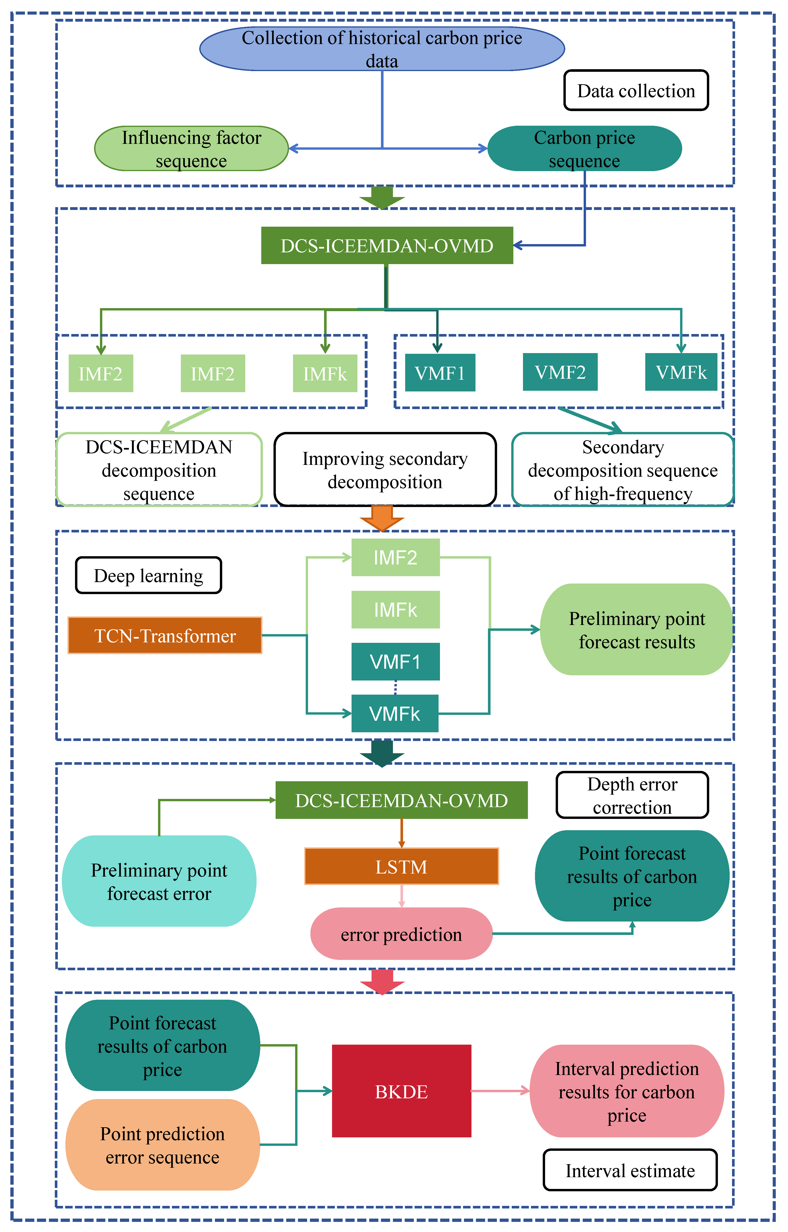
Figure 2.
Historical carbon price curve of carbon markets in Hubei and Guangdong.
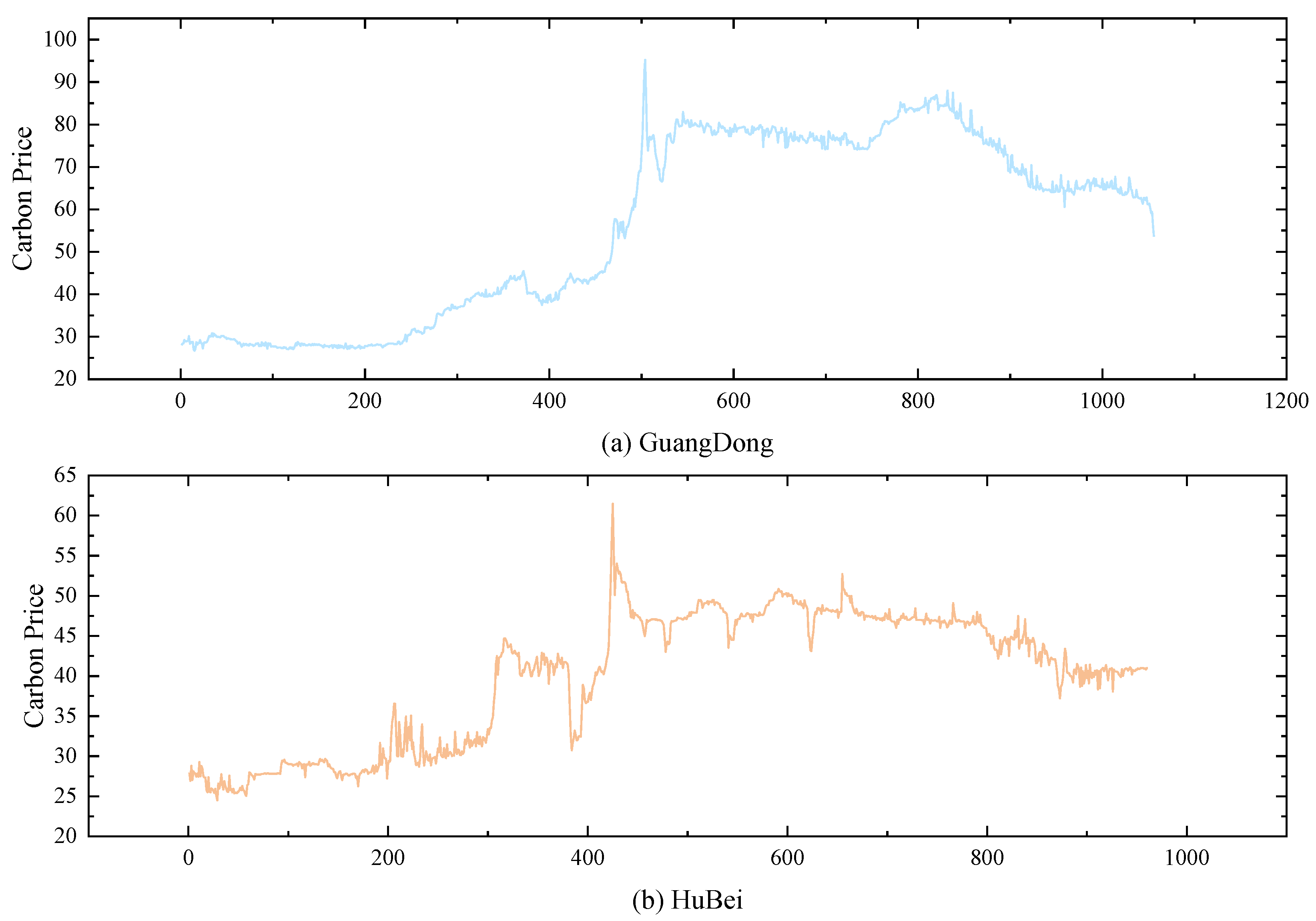
Figure 3.
Decomposition results of DCS-ICEEMDAN for the Guangdong dataset.
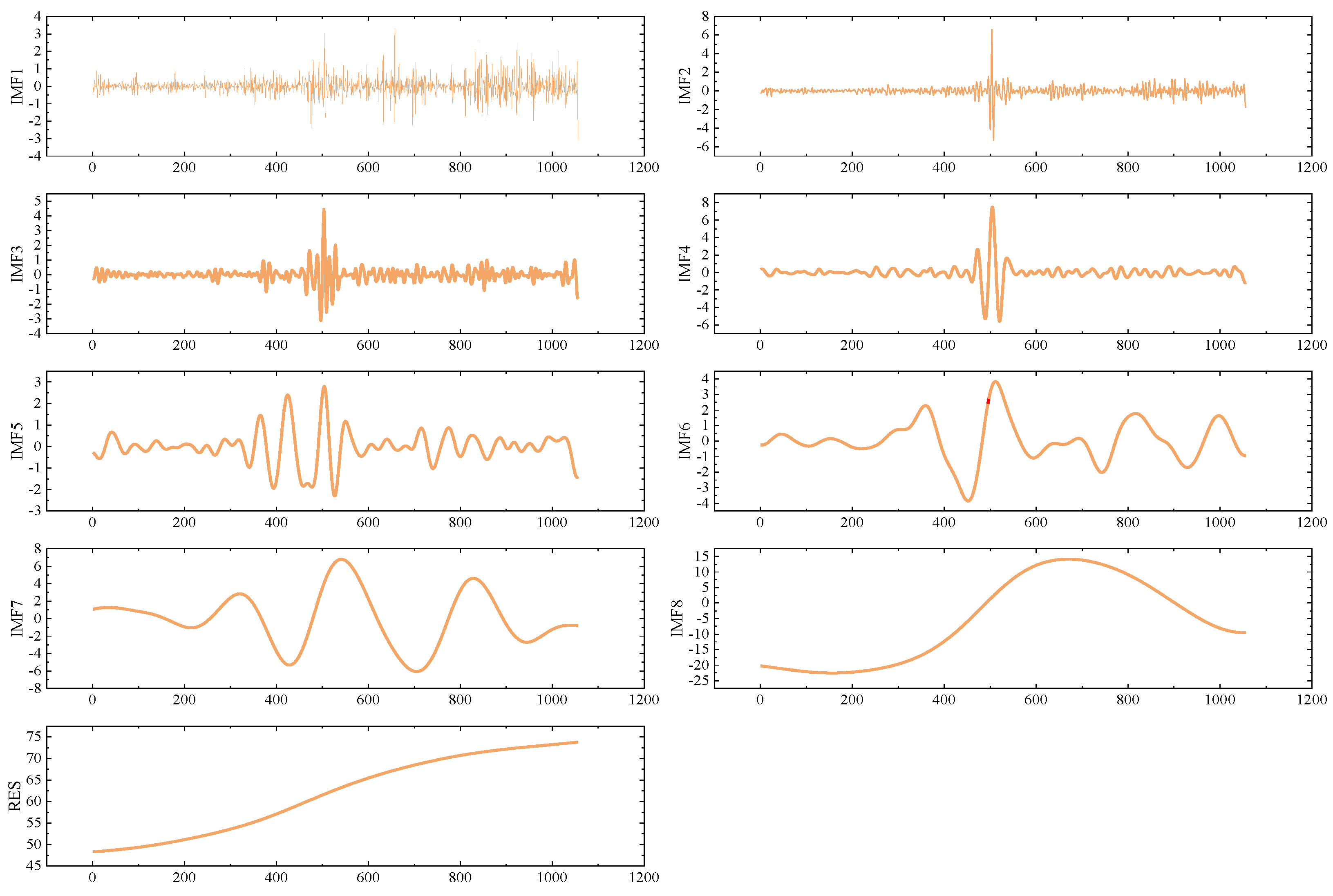
Figure 4.
Quadratic decomposition results of OVMD for the Guangdong dataset.
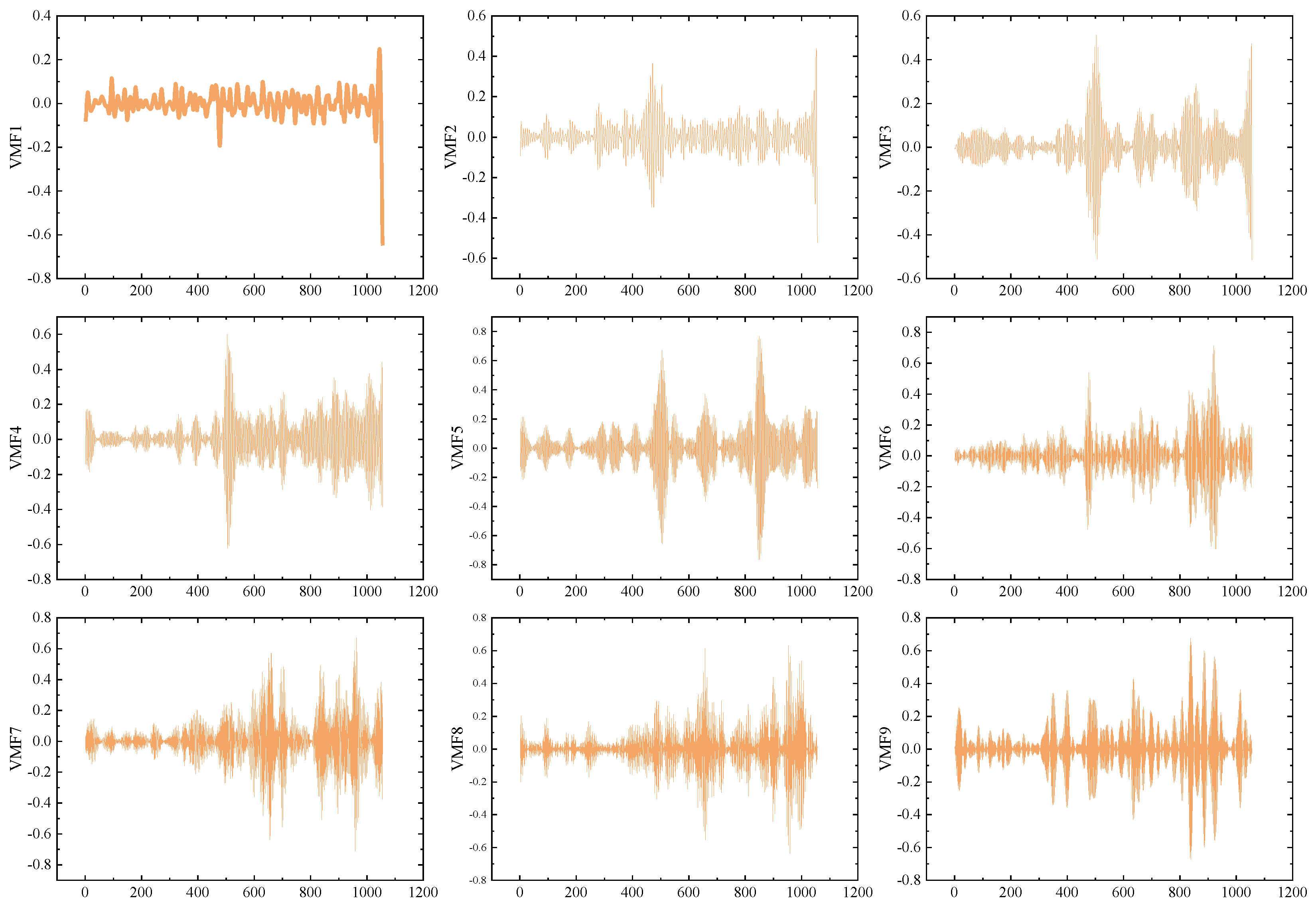
Figure 6.
Point prediction result diagram.
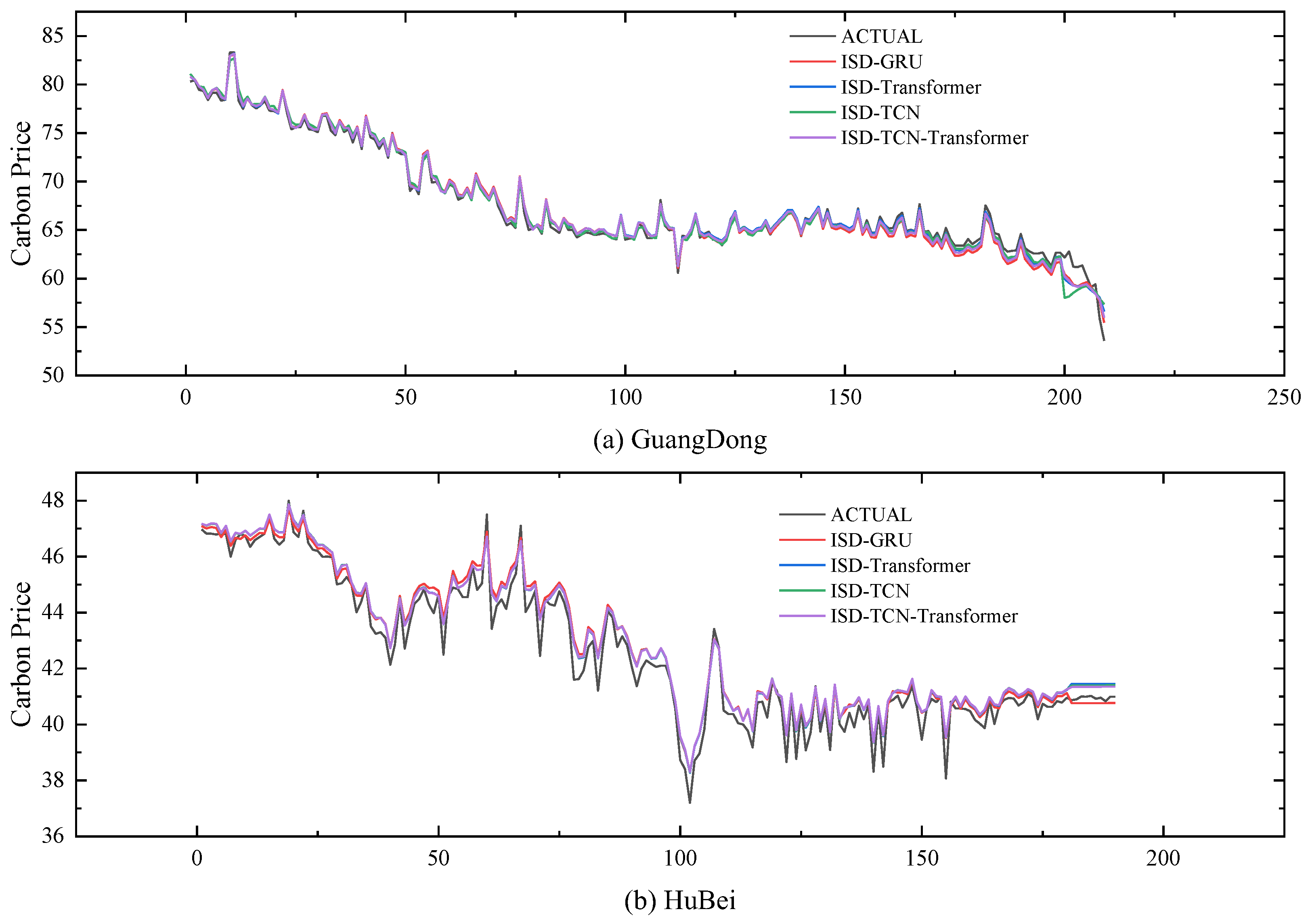
Figure 7.
Sample entropy values of error sequence and original sequence.
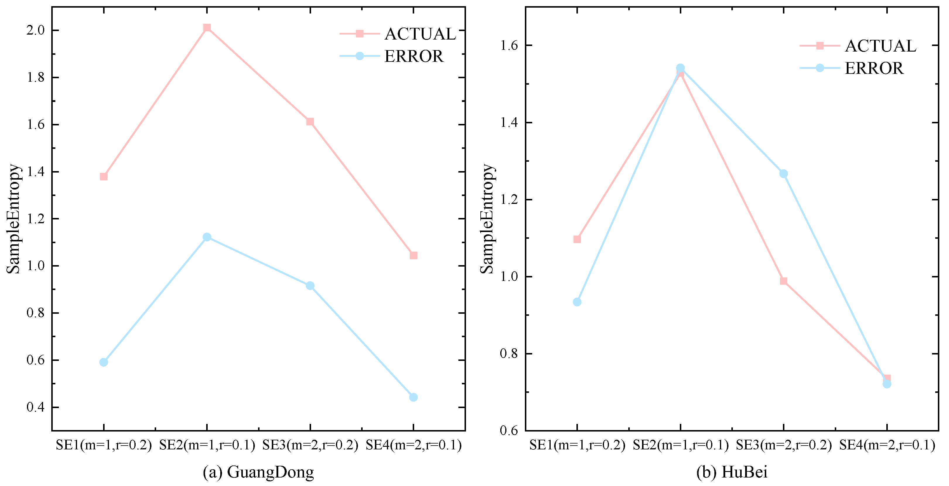
Figure 8.
Error prediction value.
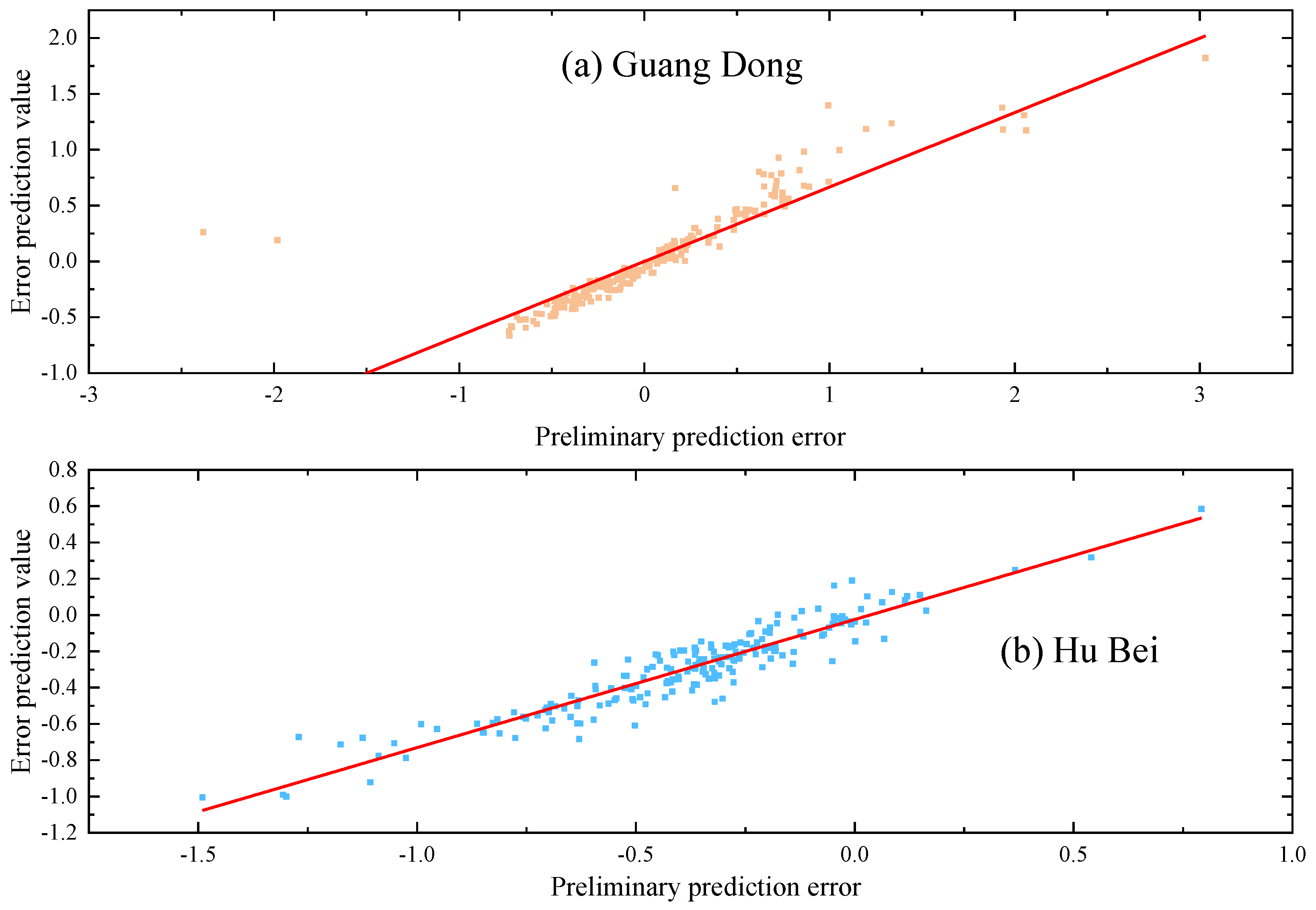
Figure 10.
Comparison of the five single-model error indicators.
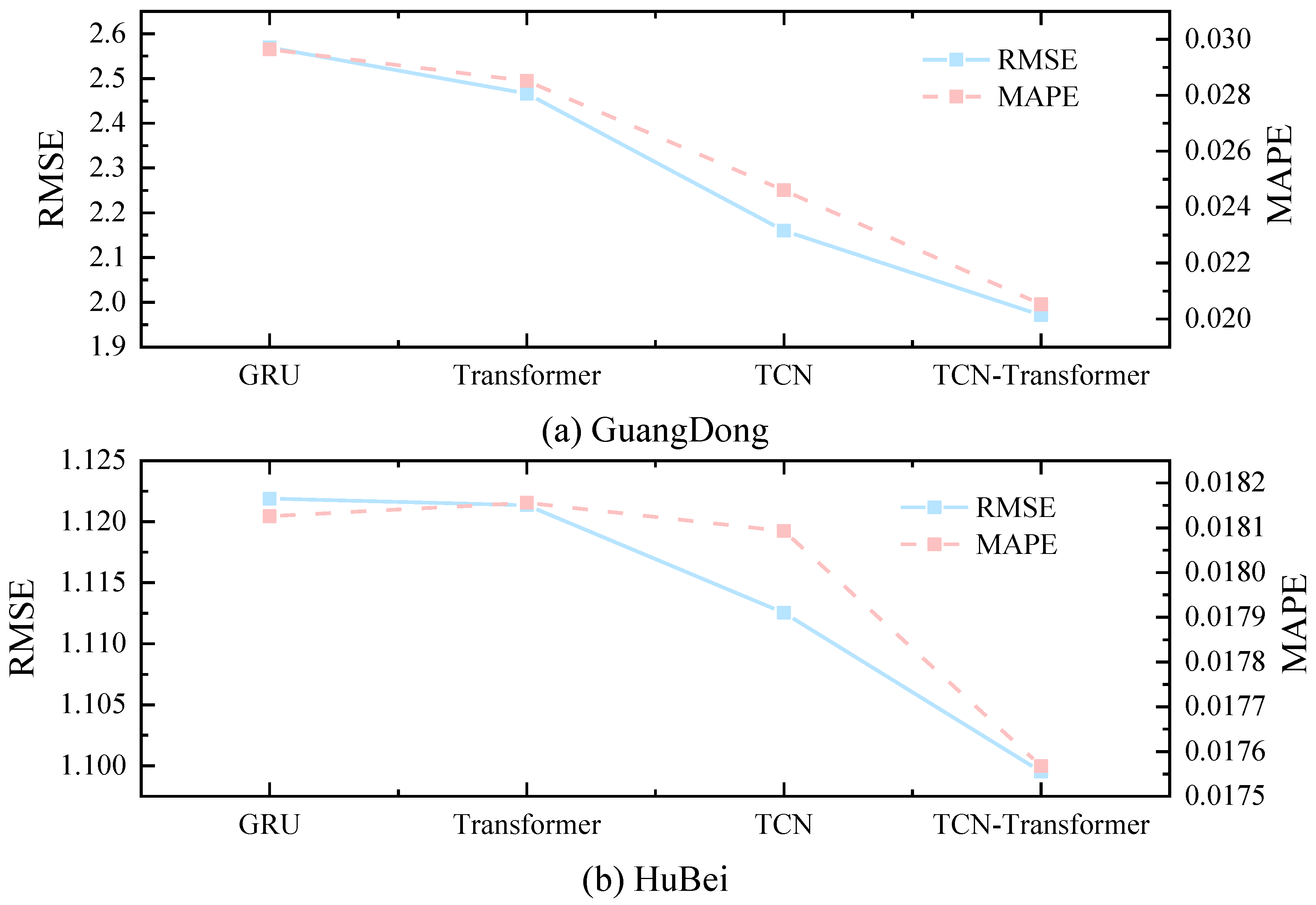
Figure 11.
Iteration curves under different optimisation algorithms.
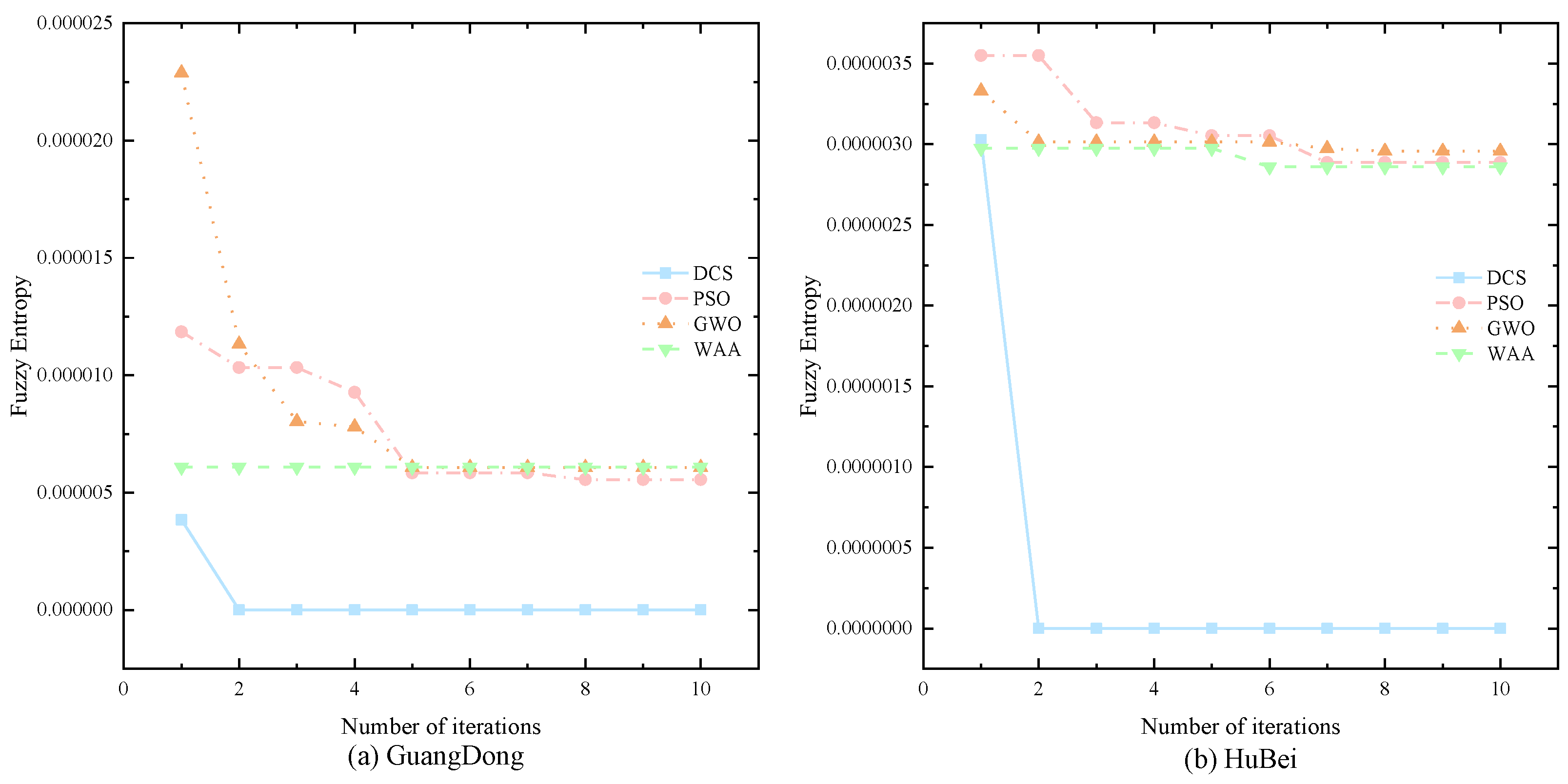
Figure 12.
RMSE values for each model with different decomposition algorithms.
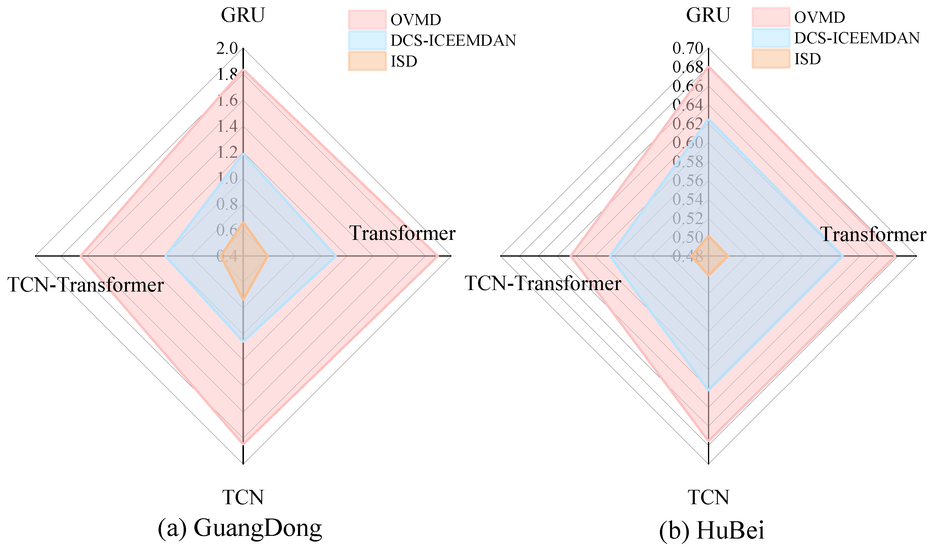
Figure 13.
Error index under different error correction algorithms.
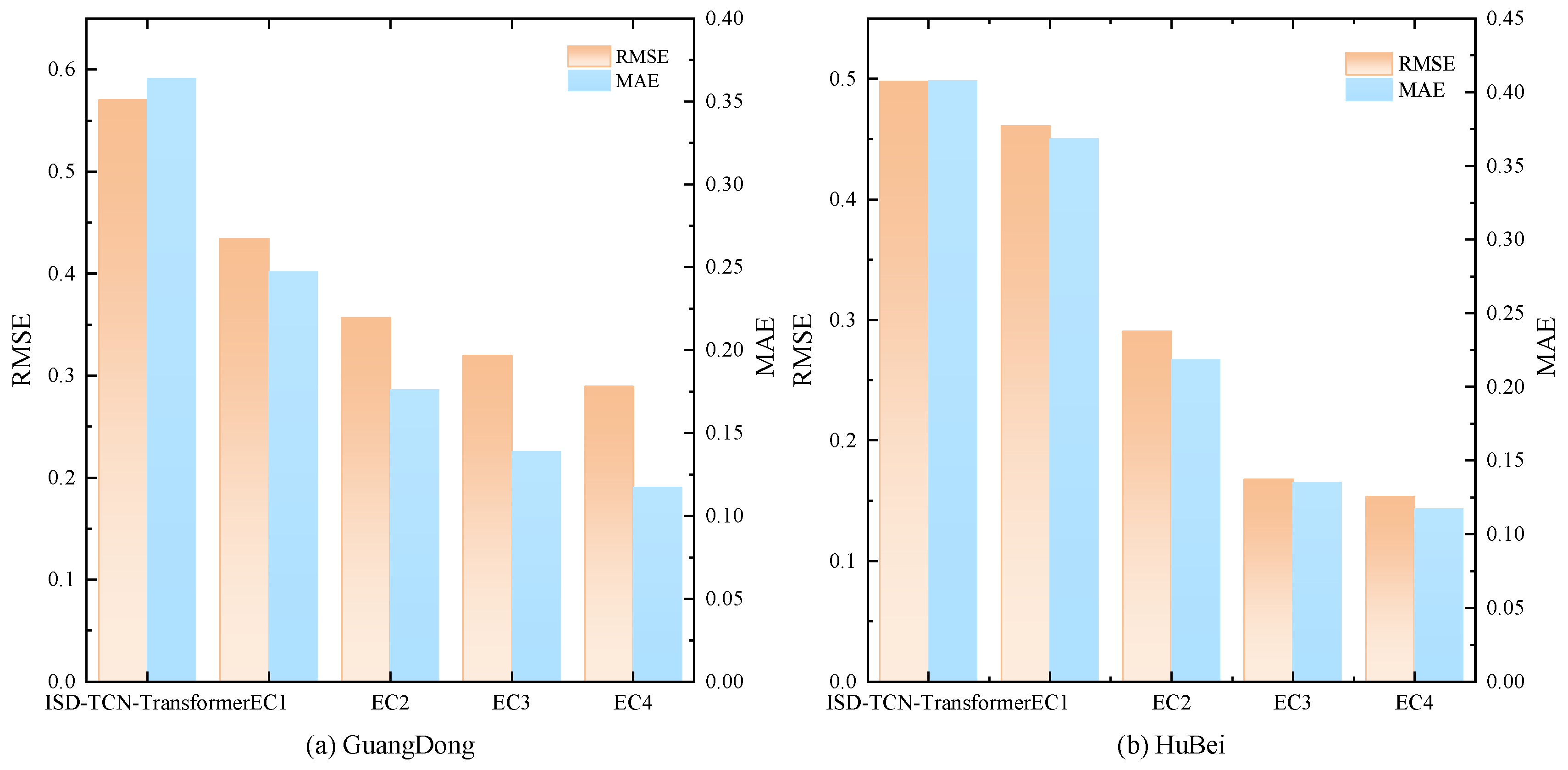
Figure 14.
Comparison of error indicators between three advanced models and the model in this paper.
Figure 14.
Comparison of error indicators between three advanced models and the model in this paper.
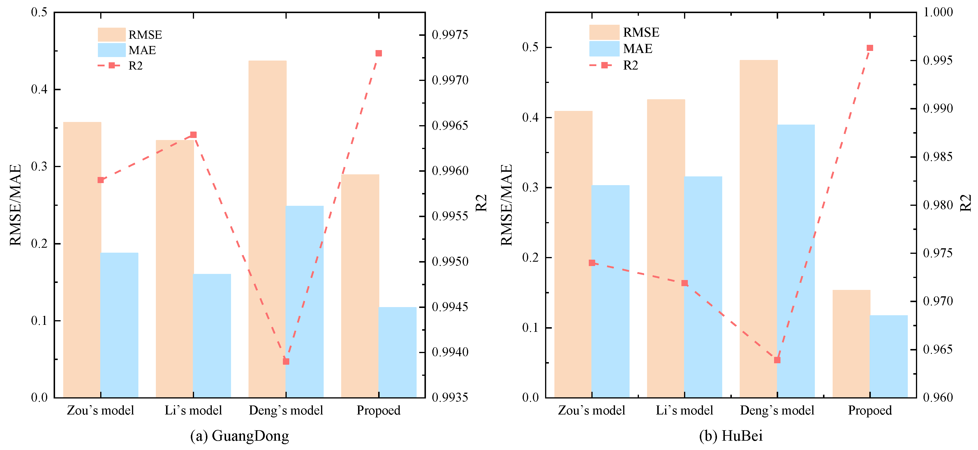
Figure 15.
Kernel density estimation results of BKDE under GuangDong datasets.
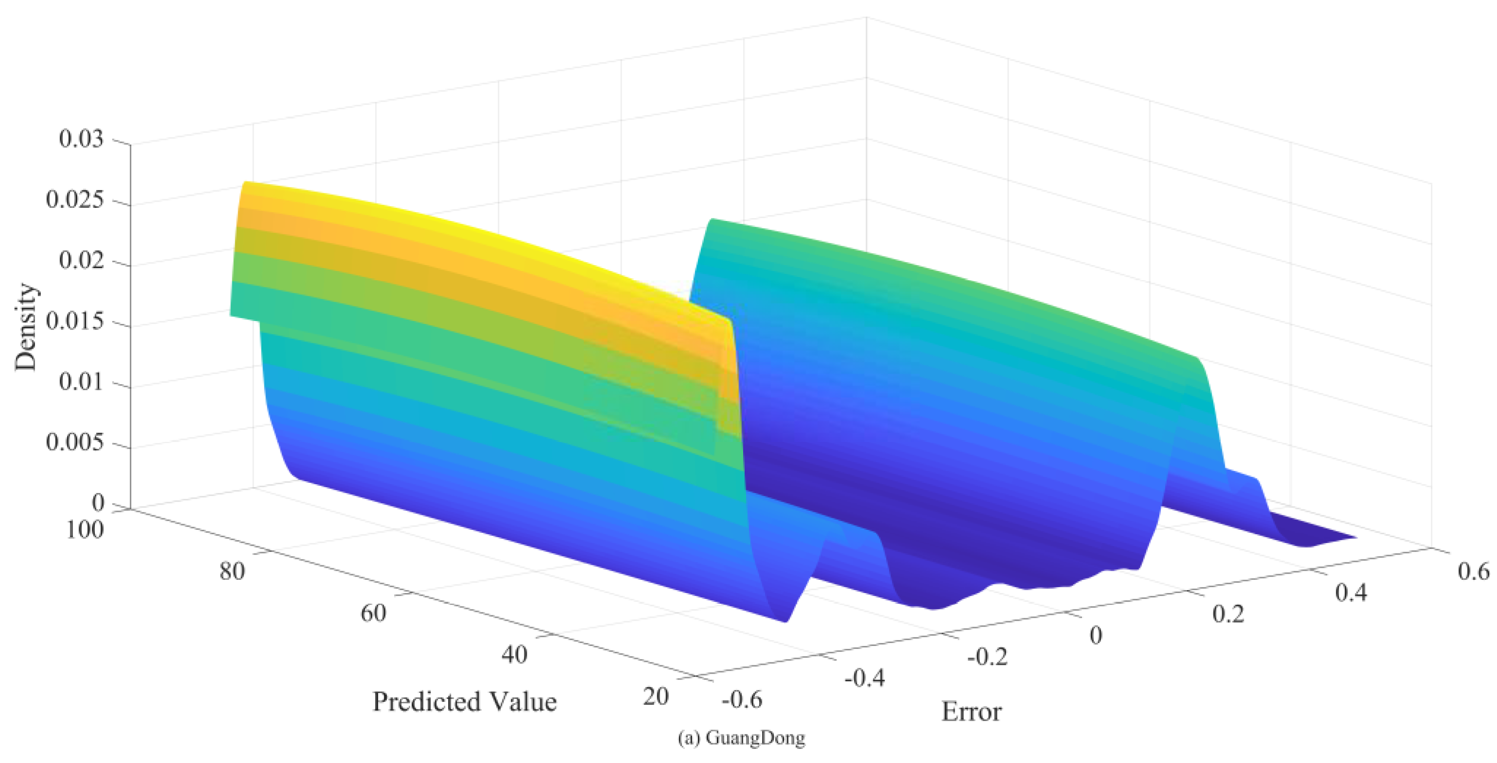
Figure 16.
Kernel density estimation results of BKDE under HuBei datasets.
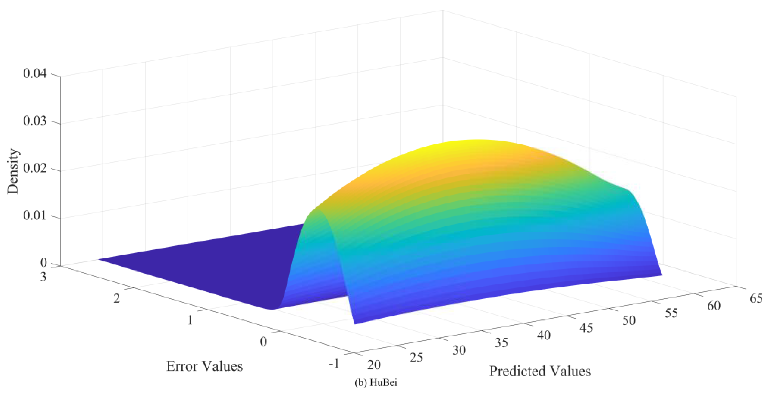

Table 1.
Dataset description in this study.
| Data | Time | Count | Mean | Std. | Min | Max |
| HuBei | 2020/1/2-2024/5/10 | 961 | 39.95 | 7.24 | 24.49 | 61.48 |
| GuangDong | 2020/1/2-2024/5/13 | 1056 | 56.12 | 19.93 | 26.67 | 95.26 |
Table 2.
Error indicator values of the five single models.
| GuangDong | HuBei | |||||||
| RMSE | MAE | MAPE | R2 | RMSE | MAE | MAPE | R2 | |
| GRU | 2.5695 | 2.1145 | 2.96% | 0.7839 | 1.1219 | 0.7804 | 1.81% | 0.8022 |
| TCN | 2.4661 | 2.0309 | 2.85% | 0.8010 | 1.1214 | 0.7815 | 1.82% | 0.8023 |
| Transformer | 2.1602 | 1.7447 | 2.46% | 0.8473 | 1.1125 | 0.7783 | 1.81% | 0.8054 |
| TCN-Transformer | 1.9711 | 1.4533 | 2.05% | 0.8729 | 1.0995 | 0.7577 | 1.76% | 0.8100 |
Table 3.
Error indicators under different optimisation algorithms in Guangdong carbon market.
| RMSE | MAE | MAPE | R2 | |
| DCS-ICEEMDAN-GRU | 1.1885 | 0.7389 | 1.05% | 0.9538 |
| DCS-ICEEMDAN-Transformer | 1.1115 | 0.6539 | 0.93% | 0.9596 |
| DCS-ICEEMDAN-TCN | 1.0572 | 0.6084 | 0.87% | 0.9634 |
| DCS-ICEEMDAN-TCN-Transformer | 0.9956 | 0.6522 | 0.94% | 0.9676 |
| PSO-ICEEMDAN-TCN-Transformer | 1.1457 | 0.7217 | 1.02% | 0.9570 |
| GWO-ICEEMDAN-TCN-Transformer | 1.0987 | 0.6737 | 0.97% | 0.9605 |
| WAA-ICEEMDAN-TCN-Transformer | 1.0414 | 0.6906 | 1.00% | 0.9645 |
Table 4.
Error indicators under different optimisation algorithms in Hubei carbon market.
| RMSE | MAE | MAPE | R2 | |
| DCS-ICEEMDAN-GRU | 0.6249 | 0.4931 | 1.14% | 0.9386 |
| DCS-ICEEMDAN-Transformer | 0.6218 | 0.4900 | 1.13% | 0.9392 |
| DCS-ICEEMDAN-TCN | 0.6218 | 0.4652 | 1.07% | 0.9392 |
| DCS-ICEEMDAN-TCN-Transformer | 0.5803 | 0.4439 | 1.02% | 0.9471 |
| PSO-ICEEMDAN-TCN-Transformer | 0.5812 | 0.4672 | 1.08% | 0.9469 |
| GWO-ICEEMDAN-TCN-Transformer | 0.5833 | 0.468 | 1.08% | 0.9465 |
| WAA-ICEEMDAN-TCN-Transformer | 0.5841 | 0.4697 | 1.08% | 0.9464 |
Table 5.
Error indicators of each model under different decomposition algorithms in Guangdong carbon market.
Table 5.
Error indicators of each model under different decomposition algorithms in Guangdong carbon market.
| RMSE | MAE | MAPE | R2 | |
| OVMD-GRU | 1.8350 | 1.4821 | 2.15% | 0.8898 |
| OVMD-Transformer | 1.8959 | 1.5632 | 2.26% | 0.8824 |
| OVMD-TCN | 1.8472 | 1.5191 | 2.20% | 0.8883 |
| OVMD-TCN-Transformer | 1.6476 | 1.3546 | 1.96% | 0.9112 |
| DCS-ICEEMDAN-GRU | 1.1885 | 0.7389 | 1.05% | 0.9538 |
| DCS-ICEEMDAN-Transformer | 1.1115 | 0.6539 | 0.93% | 0.9596 |
| DCS-ICEEMDAN-TCN | 1.0572 | 0.6084 | 0.87% | 0.9634 |
| DCS-ICEEMDAN-TCN-Transformer | 0.9956 | 0.6522 | 0.94% | 0.9676 |
| ISD-GRU | 0.6616 | 0.5020 | 0.71% | 0.9857 |
| ISD-Transformer | 0.5884 | 0.4099 | 0.58% | 0.9887 |
| ISD-TCN | 0.7338 | 0.4415 | 0.63% | 0.9824 |
| ISD-TCN-Transformer | 0.5700 | 0.3638 | 0.51% | 0.9894 |
Table 6.
Error indicators of each model under different decomposition algorithms in Hubei carbon market.
Table 6.
Error indicators of each model under different decomposition algorithms in Hubei carbon market.
| RMSE | MAE | MAPE | R2 | |
| OVMD-GRU | 0.6805 | 0.5300 | 1.23% | 0.9272 |
| OVMD-Transformer | 0.6772 | 0.5269 | 1.22% | 0.9279 |
| OVMD-TCN | 0.6755 | 0.4963 | 1.15% | 0.9283 |
| OVMD-TCN-Transformer | 0.6254 | 0.4933 | 1.14% | 0.9385 |
| DCS-ICEEMDAN-GRU | 0.6249 | 0.4931 | 1.14% | 0.9386 |
| DCS-ICEEMDAN-Transformer | 0.6218 | 0.4900 | 1.13% | 0.9392 |
| DCS-ICEEMDAN-TCN | 0.6218 | 0.4652 | 1.07% | 0.9392 |
| DCS-ICEEMDAN-TCN-Transformer | 0.5841 | 0.4697 | 1.08% | 0.9464 |
| ISD-GRU | 0.5012 | 0.3892 | 0.90% | 0.9605 |
| ISD-Transformer | 0.5006 | 0.4103 | 0.95% | 0.9606 |
| ISD-TCN | 0.5003 | 0.4093 | 0.95% | 0.9607 |
| ISD-TCN-Transformer | 0.4979 | 0.4078 | 0.94% | 0.9610 |
Table 7.
Error indicators under four error correction algorithms.
| Model | RMSE | MAE | MAPE | R2 | |
| GuangDong | ISD-TCN-Transformer-EC1 | 0.4342 | 0.2471 | 0.36% | 0.9940 |
| ISD-TCN-Transformer-EC2 | 0.3568 | 0.1760 | 0.26% | 0.9959 | |
| ISD-TCN-Transformer-EC3 | 0.3194 | 0.1388 | 0.20% | 0.9967 | |
| ISD-TCN-Transformer-EC4 | 0.2893 | 0.1171 | 0.17% | 0.9973 | |
| HuBei | ISD-TCN-Transformer-EC1 | 0.4608 | 0.3684 | 0.87% | 0.9670 |
| ISD-TCN-Transformer-EC2 | 0.2906 | 0.2184 | 0.51% | 0.9869 | |
| ISD-TCN-Transformer-EC3 | 0.1678 | 0.1352 | 0.32% | 0.9956 | |
| ISD-TCN-Transformer-EC4 | 0.1534 | 0.1172 | 0.28% | 0.9963 |
Table 8.
This paper models and error indicators of three advanced models.
| Model | RMSE | MAE | MAPE | R2 | |
| GuangDong | Zou’s model | 0.3570 | 0.1876 | 0.28% | 0.9959 |
| Li’s model | 0.3337 | 0.1602 | 0.24% | 0.9964 | |
| Deng’s model | 0.4367 | 0.2485 | 0.37% | 0.9939 | |
| Propoed | 0.2893 | 0.1171 | 0.17% | 0.9973 | |
| HuBei | Zou’s model | 0.4088 | 0.3028 | 0.71% | 0.9740 |
| Li’s model | 0.4251 | 0.3152 | 0.74% | 0.9719 | |
| Deng’s model | 0.4815 | 0.3893 | 0.91% | 0.9639 | |
| Propoed | 0.1534 | 0.1172 | 0.28% | 0.9963 |
Table 9.
The advantages and disadvantages of the three advanced models.
| Name | Published year | Major contribution | Disadvantages compared with the proposed model |
| Zou’s model | 2024 | •CEEMD-VMD secondary decomposition technology is adopted •Optimize LSTM with IPSO |
•Ignore the importance of CEEMD and VMD parameter selection •Neglects interval estimation |
| Li’s model | 2025 | •Apply one decomposition technique to error correction •The decomposed components were classified |
•The secondary decomposition technique is not considered to be introduced into the error correction algorithm •No secondary decomposition technology is used |
| Deng’s model | 2025 | •An enhanced secondary decomposition technique is proposed to solve the problem of over-decomposition of secondary decomposition |
•Neglects interval estimation •The adaptive ability of secondary decomposition technology is not strengthened |
Table 10.
Interval indicator values at 95 % confidence intervals for different interval estimation algorithms.
Table 10.
Interval indicator values at 95 % confidence intervals for different interval estimation algorithms.
| GuangDong | HuBei | |||||
| PICP | PINAW | CWC | PICP | PINAW | CWC | |
| T Location Scale | 0.7630 | 0.0078 | 0.1468 | 0.7172 | 0.0047 | 0.1284 |
| Logistic | 0.7393 | 0.0073 | 0.1440 | 0.7475 | 0.0050 | 0.1299 |
| Normal | 0.7962 | 0.0082 | 0.1493 | 0.7172 | 0.0047 | 0.1283 |
| GMM | 0.7346 | 0.0075 | 0.1449 | 0.7071 | 0.0047 | 0.1282 |
| KDE | 0.7536 | 0.0077 | 0.1464 | 0.7071 | 0.0049 | 0.1296 |
| BKDE | 0.9617 | 0.0336 | 0.0336 | 0.9842 | 0.0784 | 0.0784 |
Disclaimer/Publisher’s Note: The statements, opinions and data contained in all publications are solely those of the individual author(s) and contributor(s) and not of MDPI and/or the editor(s). MDPI and/or the editor(s) disclaim responsibility for any injury to people or property resulting from any ideas, methods, instructions or products referred to in the content. |
© 2025 by the authors. Licensee MDPI, Basel, Switzerland. This article is an open access article distributed under the terms and conditions of the Creative Commons Attribution (CC BY) license (http://creativecommons.org/licenses/by/4.0/).
Copyright: This open access article is published under a Creative Commons CC BY 4.0 license, which permit the free download, distribution, and reuse, provided that the author and preprint are cited in any reuse.


