Submitted:
07 October 2025
Posted:
08 October 2025
You are already at the latest version
Abstract
As an important energy and chemical raw material in the world, the price fluctuation of crude oil has been affecting the economic level of all countries in the world, however, the crude oil price has a strong nonlinear trend and chaotic characteristics, which makes the crude oil price prediction very challenging. Based on this, this paper proposes a three-stage forecasting model based on "two-mode decomposition-multi-scholar forecasting-nonlinear integration". In this study, we first use bimodal decomposition to obtain two different sets of multiscale components to show the detailed features of crude oil prices from different perspectives, then we use long-short-term neural network (LSTM), kernel extremum learning machine (KELM), and gated recursive unit (GRU) to learn the deeper features of the two sets of components from different aspects, and finally, we use the multi-objective viscosity optimization algorithm (MOSMA) and extreme gradient Boosting Tree (XGBoost) to integrate the six models and obtain point prediction and interval prediction results. The simulation experimental results show that compared with the comparison models, the bimodal decomposition can better reflect the detailed information of the original series of oil price and realize the complementary advantages between different decomposition methods; the nonlinear integration can effectively combine the advantages of different models and improve the prediction accuracy.
Keywords:
ensemble forecasting
; multi-objective optimization
; nonlinear ensemble
; bimodal decomposition
; crude oil price forecasting
1. Introduction
Crude oil, as a crucial strategic resource globally, significantly impacts the world economy with its price fluctuations. However, due to a series of unconventional events such as political, economic, technological, and weather-related factors(Dai, Kang and Hu 2021, Gong et al. 2021), crude oil prices exhibit non-linearity and high volatility. Consequently, accurately predicting the trend of oil prices and mitigating potential risks in the future have become a focal point in academic research. In order to effectively forecast oil price volatility, scholars have proposed econometric models such as Ordinary Least Squares (OLS) (Yin and Yang 2016), Autoregressive Integrated Moving Average (ARIMA) (Mo and Tao 2016), Vector Autoregression (VAR)(Baumeister and Kilian 2012, Drachal 2021), Vector Error Correction Model (VECM)(Berrisch et al. 2023, Chen, Lu and Ma 2022), and Generalized Autoregressive Conditional Heteroskedasticity (GARCH) (Ambach and Ambach 2018, Lux, Segnon and Gupta 2016). These models derive short-term predictions of oil prices by fitting the impact relationships between oil prices and relevant variables. Although econometric models offer strong explanatory power for oil price volatility, they are limited by the assumption of linearity among time series, unable to capture nonlinear trends in oil prices, and are susceptible to noise interference in oil price data.
Therefore, in order to reduce noise, decrease prediction complexity, and enhance prediction accuracy, scholars have begun employing decomposition algorithms such as Empirical Mode Decomposition (EMD) (Yang, Zhang and Jiang 2019), Wavelet Transform (WT) (Lin et al. 2022), and Variational Mode Decomposition (VMD)(Zhang et al. 2023) to mitigate the volatility and noise in the time series of oil prices. For instance, (Wu, Wang and Hao 2022) utilized HI-CEEMD for data preprocessing followed by ESN optimized with MOIWCA to obtain predictive results, demonstrating that models subjected to outlier detection and CEEMD decomposition significantly improved predictive capabilities. (Wu et al. 2023) applied VMD-IGJO-LSTM and ICEEMDAN-GRU for predicting the original data and error sequences respectively, with experimental results indicating that VMD and ICEEMDAN effectively enhanced model predictive accuracy. (Wang and Fang 2022) employed WT-FNN for oil price prediction, revealing that the predictive performance of the WT-FNN model surpassed that of the FNN model and the unaltered model. These studies collectively suggest that decomposition algorithms can effectively mitigate the chaotic characteristics of oil price sequences and enhance predictive accuracy. However, single-mode decomposition methods like CEEMD, VMD, and WT suffer from weak nonlinear coupling capabilities, low decomposition precision, and inherent flaws in each decomposition algorithm(Bi et al. 2023).
In order to better capture the nonlinear trends in oil prices, artificial intelligence models have gradually replaced traditional econometric models, becoming the mainstream predictors in oil price forecasting. For instance, (Jovanovic et al. 2022) utilized an improved version of the Salp swarm algorithm optimized Long Short-Term Memory (LSTM) to predict the WTI oil prices, achieving promising results. (Wang, Xia and Lu 2022) initially employed a Support Vector Machine (SVM) optimized by a Genetic Algorithm (GA) to forecast oil prices, then utilized a Generalized Regression Neural Network (GRNN) to predict the residual sequence, ultimately obtaining the oil price forecast. Experimental results demonstrate that GA-SVR-GRNN can fully leverage the advantages of nonlinear prediction, exhibiting robust predictive capabilities.
Although artificial intelligence models typically utilize iterative algorithms to gradually approach the optimal solution by continuously adjusting parameters, they can better fit nonlinear trends. However, actual oil price time series exhibit complex nonlinear structures and chaotic characteristics, making it difficult for individual models to fully capture the complex information behind oil price time series. Furthermore, artificial intelligence models are prone to overfitting and falling into the trap of local optima. Hence, the performance of prediction models based on individual artificial intelligence sometimes falls short of expectations.
Therefore, with the further development of forecasting techniques, ensemble models integrating multiple artificial intelligence models have gradually become one of the hotspots in oil price prediction. Ensemble models can combine the strengths of multiple predictors, fully capturing all features in the oil price series, and offering higher predictive accuracy and applicability. For example, (Wang et al. 2020) employed the Artificial Bee Colony (ABC) algorithm to combine the predictions of Linear Regression (LR), Artificial Neural Network (ANN), and Support Vector Machine (SVM). Their conclusion indicates that the multi-granularity heterogeneous method based on the ABC algorithm is significantly superior to the single-granularity heterogeneous method. (Hao et al. 2022) utilized the Non-dominated Sorting Genetic Algorithm II (NSGA-II) to dynamically combine the predictions of 14 forecasters. Experimental results demonstrate that dynamic weight combination is significantly superior to static weight combination. In addition, ensemble methods are also commonly used for interval estimation. Unlike interval estimation methods such as Kernel Density Estimation (KDE) (Wu et al. 2023) and Bootstrap (Zhao et al. 2021), which require certain assumptions, this method can directly generate interval estimates without any assumption. For instance, (Wang et al. 2020) utilized the Improved Adaptive Grey Wolf Optimizer with Cuckoo Search (AGWOCS) to combine the interval prediction results of five models: BPNN, LSTM, BiLSTM, GPR, and Lasso, to obtain interval estimation. The results indicate that this method can achieve better results than conventional interval estimation methods. Although ensemble strategies can leverage the advantages of various models to improve the accuracy and applicability of models, existing methods typically adopt weighted ensemble methods. However, as far as we know, nonlinear ensemble forecasting performs better in terms of modeling difficulty and ensemble performance than weighted ensemble methods(Yang, Hao and Hao 2023). Therefore, further research is needed on the role of nonlinear ensemble forecasting in the field of oil price prediction.
In the aforementioned context, a multi-step crude oil futures price forecasting system is proposed based on dual-mode decomposition and nonlinear ensemble to address issues such as the weak nonlinear coupling ability and low decomposition accuracy of single-mode decomposition algorithms, as well as the poor applicability of single models, thereby enhancing the predictive capability of the model.
The model first employs two decomposition algorithms to process oil price sequences, followed by predictions using three machine learning algorithms. Subsequently, a nonlinear ensemble combines the predictions of six models. Finally, different evaluation metrics are selected to analyze the predictive performance, verifying the effectiveness and superiority of the proposed forecasting model.
The main contributions of this study are as follows:
1.Introduction of dual-mode decomposition technology, constructing two multiscale components generated by different mathematical mechanisms to achieve complementary advantages of the two decomposition algorithms, thereby achieving accurate oil price prediction.
2.Utilization of a multi-objective slime mold algorithm (MOSMA) and XGBoost for ensemble forecasting framework, considering both prediction error and variance, to build a multi-objective optimized nonlinear ensemble model, effectively improving the model’s generalization ability and better realizing crude oil price prediction.
3.Simultaneous introduction of decomposition algorithms and ensemble strategies to jointly enhance the predictive accuracy of the model.
The remaining sections of the paper are organized as follows. Section II details the design of the model and the methodology of the corresponding module of the paper. Simulation experiments and related analysis are given in Section III. We will further evaluate our prediction system in Section IV. Section V summarizes the whole paper.
2. Materials and Methods
2.1. Forecasting Framework
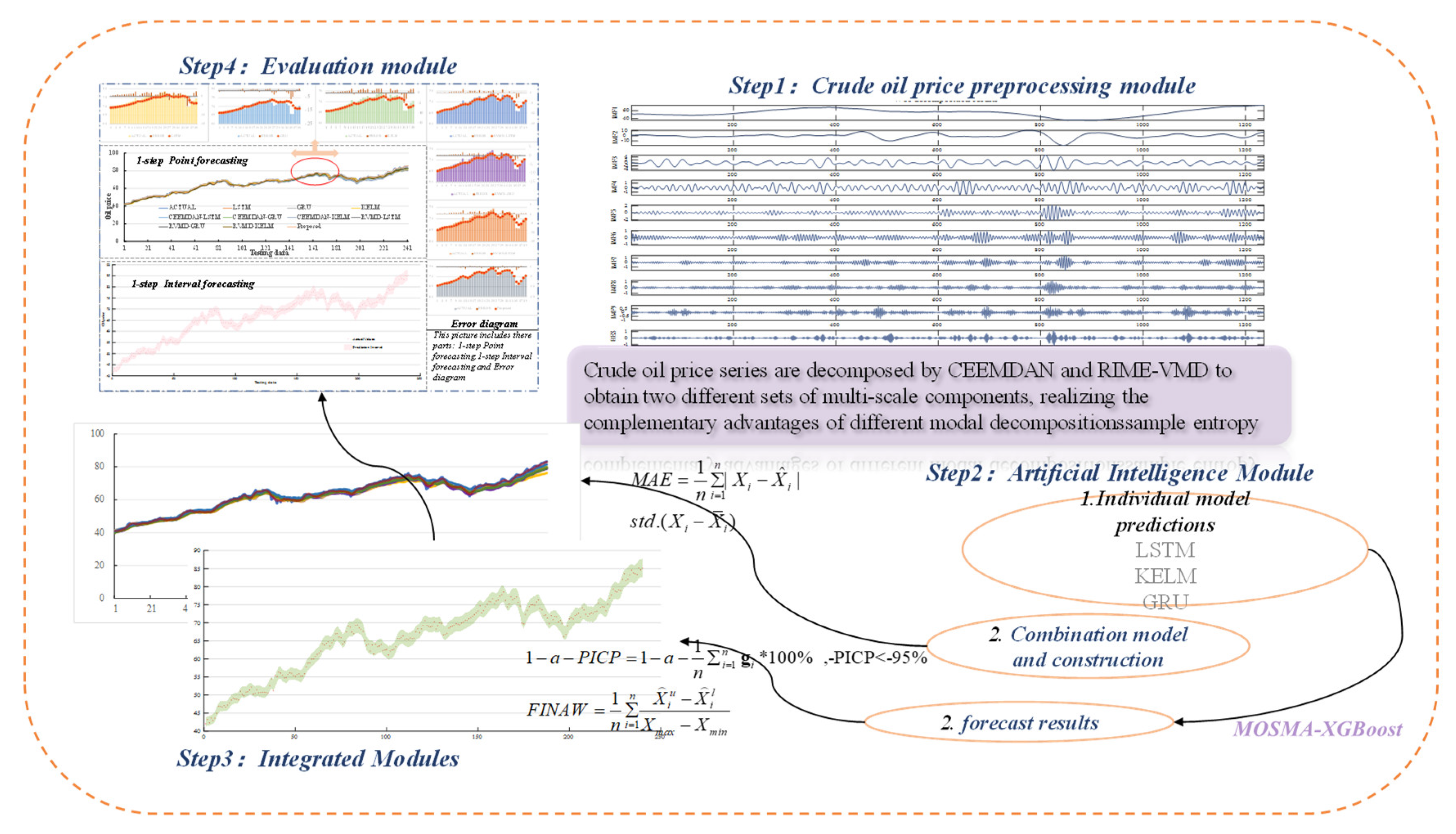
In order to obtain accurate point prediction and suitable interval prediction results, an ensemble forecasting model was developed. The model is designed with three modules, which are data preprocessing module, artificial intelligence module, and ensemble module. The data preprocessing module reduces the noise interference of the oil price series, the artificial intelligence module provides the prediction results of three forecasters, LSTM, KELM and GRU, which provides a strong foundation for the next step of ensemble forecasting, and the ensemble module uses nonlinear ensemble to provide more excellent results for point and interval forecasting. The developed modeling details are shown in Figure 1 and the details can be summarized as follows:
Stage 1: Extraction of the main features of the raw oil price data. A data preprocessing module is proposed and applied to extract the main information of the raw data. The module employs the VMD algorithm based on RIME optimization and CEEMDAN to decompose the raw data to obtain the eigenmode components and residual terms of two different frequencies.
Stage 2: Obtaining the prediction results of different models. In this stage, three artificial intelligence models are applied to predict the oil price data after two decomposition algorithms.
Stage 3: Nonlinear ensemble. Apply MOSMA-XGBoost to ensemble the six prediction results to get point prediction results and interval prediction results.
Figure 1.
Model flow chart.
2.2. Data Preprocessing Module
2.2.1. Rime Optimization Algorithm
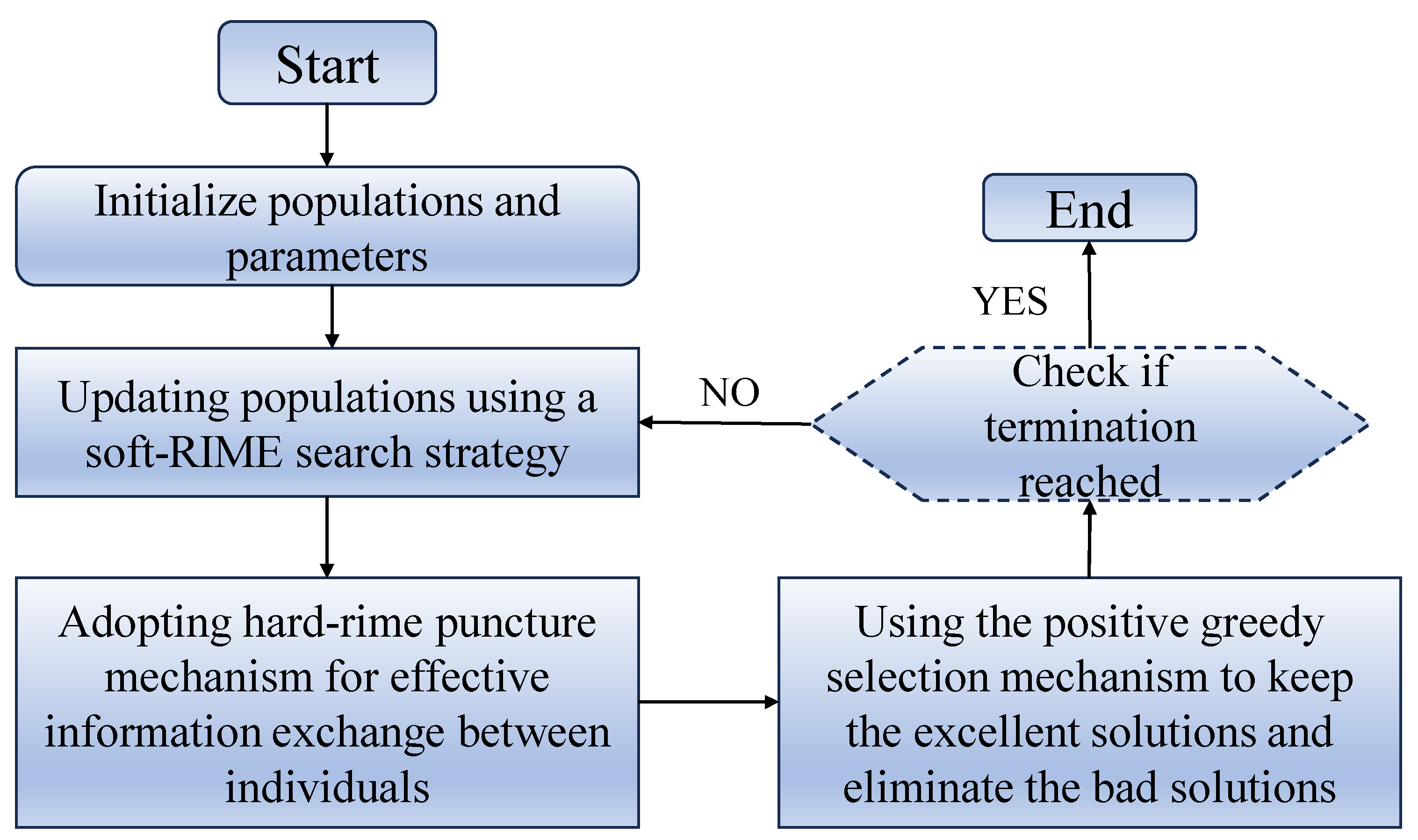
Rime optimization algorithm (RIME) was proposed by Hang Su in February 2023, which was inspired by the haze ice growth mechanism and proposed a frost ice search strategy for algorithmic search by simulating the motion of soft frost ice particles. The algorithm is composed as follows.
Rime optimization algorithm (RIME) was proposed by Hang Su in February 2023, which was inspired by the haze ice growth mechanism and proposed a frost ice search strategy for algorithmic search by simulating the motion of soft frost ice particles. The algorithm is composed as follows.
1, Frost ice cluster initialization. Where are the ordinal number of the RIME agent and the ordinal number of the frost ice particles, respectively, R stands for rime-population, and is used to represent the fitness value of the agent in the meta-heuristic algorithm.
2, Soft freezing fog search strategy. According to the five kinematic properties of the freezing fog particles, the condensation process of each freezing fog particle was simulated concisely and the position of the freezing fog particles was calculated, as shown in equation (3).
where is the new position of the updated particle. is the particle of the best fogging agent in the j-th fogging population. The parameter is a random number in the range of (-1,1) and controls the direction of particle movement, will change with the increase of iteration number as shown in equation (4). is the environment factor, which follows the number of iterations to simulate the influence of the external environment and is used to ensure the convergence of the algorithm, as shown in equation (5). is the adhesion degree which is a random number in the range of (0,1) and is used to control the distance between the centers of two fog particles. and are the upper and lower limits of the escape space, respectively, which limit the effective region of particle motion. is the attachment coefficient, which affects the coalescence probability of the intelligences and increases with the number of iterations as shown in equation (6).
where represents the current iteration number and the maximum iteration number, respectively.
where the default value of is 5 to control the number of segments of . The default value of is 5.
3, Hard Freeze Piercing Mechanism. Inspired by the puncture phenomenon, a hard freezing fog puncture mechanism is proposed, which can be used to update the algorithms between intelligences so that the particles of the algorithms can be exchanged and the convergence of the algorithms and the ability to jump out of the local optimum can be improved. The interparticle replacement formula is shown in equation (7).
denotes the normalized value of the current intelligent body fitness value.
4, Positive greedy selection mechanism. The specific idea is to compare the fitness value of the intelligent body after the update with the fitness value of the intelligent body before the update, and if the fitness value after the update is better than the value before the update, the replacement occurs and replaces the solutions of both intelligences at the same time.
Figure 2.
Flowchart of the RIME algorithm.
2.2.2. Variational Modal Decomposition
VMD, proposed by Dragomiretskiy and Zosso to address the mode-mixing issues in EMD, presents a novel and sophisticated signal decomposition method. Unlike EMD and EEMD, VMD is a non-recursive approach that effectively avoids mode-mixing, separating distinct features within the original signal. It demonstrates superior decomposition efficacy and higher robustness. However, the number of modes (K) and penalty factor for VMD need to be pre-set. The mode number, K, determines the number of decompositions, while the penalty factor, α, controls the smoothness between modes. Therefore, appropriate values for K and α are essential for more effective signal decomposition and improved predictive performance. To efficiently select these two parameters, this study employs RIME with the minimization of sample entropy as the optimization target.
2.2.3. Adaptive Noise-Embedded Empirical Mode Decomposition
The Adaptive Noise-Embedded Empirical Mode Decomposition (CEEMDAN), as an improved algorithm of Empirical Mode Decomposition (EMD), has been successfully applied to signal denoising. In contrast to wavelet and Fourier decomposition algorithms, the CEEMDAN algorithm does not require assumptions of data stationarity and linearity, thus offering a broader range of applications and clear advantages in handling non-stationary time-series data (Torres et al. 2011).
2.3. Artificial Intelligence Module
2.3.1. Long Short-Term Memory Networks
In order to address the issue of vanishing or exploding gradients in Recurrent Neural Networks (RNNs), (Hochreiter and Schmidhuber 1997) introduced gate mechanisms to control the flow and loss of features. Here, the input gate is responsible for accepting recent relevant information, the forget gate selectively discards distant or irrelevant information, and the output gate produces output based on the current state.
2.3.2. Gated Recurrent Units
Both GRU and LSTM employ gate mechanisms to control the update and retention of hidden states. However, GRU has a simpler structure, consisting of only two gates: the reset gate and the update gate. The reset gate regulates the retention and discard of information within the hidden state, while the update gate controls the proportion between the previous timestep’s hidden state and the current timestep’s candidate hidden state. It also governs the retention and discard of information within the current timestep’s hidden state (Wu et al. 2020).
2.3.3. Kernel Extreme Learning Machine
KELM is a machine learning algorithm based on perceptrons, utilizing randomly generated weights and biases during the training process. Unlike traditional perceptron algorithms, KELM employs a kernel function to map input data, enabling it to handle nonlinear data prediction problems.
2.4. Ensemble Module
2.4.1. XGBoost
XGBoost, proposed by Tianqi Chen in 2014, is a machine learning algorithm that employs a forward additive approach to gradually build an ensemble model consisting of multiple decision trees. Each tree is fitted based on the residuals of the previous trees. Additionally, XGBoost incorporates regularization techniques, such as column subsampling and row subsampling, to mitigate the risk of overfitting.
2.4.2. Multi-Objective Slime Mould Optimization Algorithm
The multi-objective slime mould optimization algorithm utilized here is a novel multi-objective random search optimization algorithm proposed by (Premkumar et al. 2021) in 2021. This algorithm incorporates the convergence mechanism of slime mould optimization, updating the population through approaches like approach, engulf, and grip in each iteration, thus exhibiting strong global search capabilities. MOSMA operates on the principles of non-dominated solution sorting and crowding distance sorting to maintain population diversity, selecting superior individuals from the slime mould population through elite non-dominated sorting.
2.4.3. Ensemble Prediction Module
To leverage the strengths and address the limitations of multiple models effectively, the ensemble prediction model combines the predictions from three hybrid models based on CEEMDAN and three hybrid models based on RIME-VMD. Introducing a novel ensemble forecaster based on multi-objective optimization, the integration of multi-objective optimization with artificial intelligence prediction models is proposed.
Specifically, recognizing that the XGBoost model provides superior forecasting and real-time learning, it is chosen as the foundation for the ensemble forecaster. While XGBoost has certain advantages over traditional artificial neural network models, it also shares limitations with other artificial neural network models. The performance of XGBoost is significantly influenced by its four initial parameters, and if these parameters are not suitable for specific data, the predictive results may be suboptimal. To address this issue, researchers have started incorporating artificial intelligence optimization into the model development process. In this context, the optimizer for XGBoost proposed in Section 2.4.2, based on MOSMA, serves as the foundation for developing an ensemble forecaster rooted in a multi-objective optimizer. It is crucial to note that point prediction and interval prediction have different evaluation criteria, necessitating the definition of distinct objective functions for point prediction and interval prediction.
Objective Function for Oil Price Point Forecasting
In order to improve the accuracy and stability of oil price point forecasting, therefore the accuracy and stability metrics are used to optimize the objective function which is defined as shown in Equation 8, where and are the actual and predicted values
Objective Function for Oil Price Interval Forecasting
For oil price interval forecasting, higher coverage probability and narrower interval width are essential in engineering applications. Therefore, in order to improve the coverage probability and interval width for oil price interval forecasting, the coverage probability and interval width metrics are used to optimize the objective function, which is defined as shown in Eq.9. where 1- is the expected probability, and represent the upper and lower bounds, where when the actual value falls into the upper and lower bounds of the interval estimation, it is 1 and 0 otherwise
2.5. Error Evaluation Criteria
The study uses five point prediction indicators, RMSE, MAE, MAPE, R2, and VAR, to evaluate the prediction effect of each model, in addition, three interval prediction indicators, PICP, PINAW, and CWC, are also used to evaluate the interval prediction effect of the model. Here, represent the upper and lower bounds of the ith prediction value, is 0.1, is 6, is 15, and is 0.9, respectively
3. Case Study
3.1. Data Sources and Descriptive Analysis
In this study, the crude oil futures prices of WTI and Brent for each trading day from January 3, 2017 to October 20, 2021 are selected as the object of the study, and the interpolation method is used to correct some missing values and outliers. The first 80% of them were used as the training set and the last 20% as the test set. Subsequently, the data sets of WTI and Brent crude oil futures prices were analyzed descriptively respectively. The results of the descriptive analysis are shown in Table 1.
Figure 3.
Crude oil prices for WTI and Brent from 2017/1/3 to 2021/10/20.
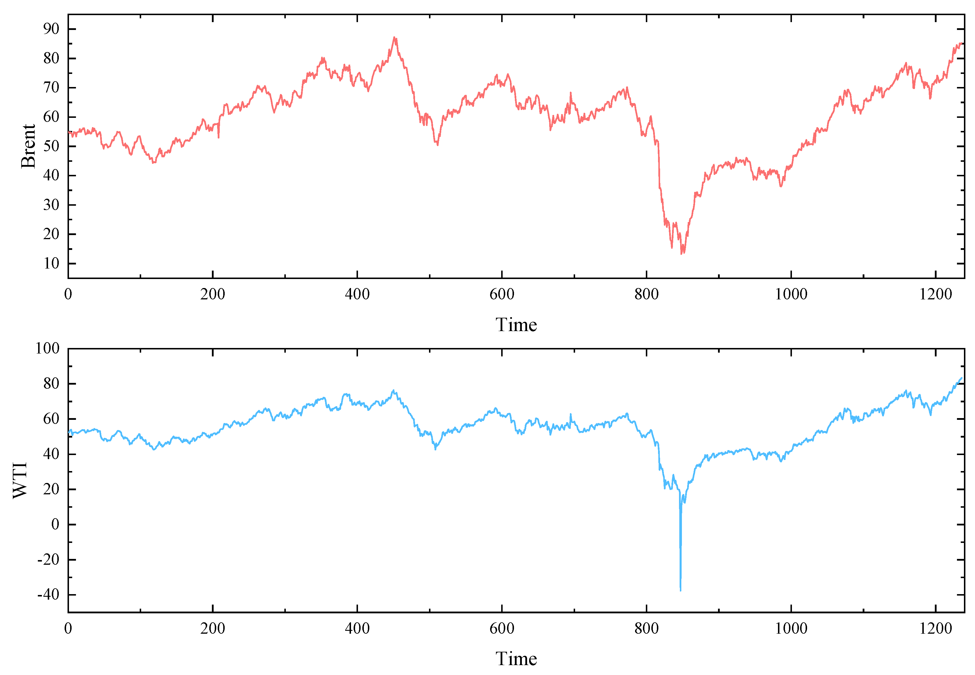

Table 1.
Descriptive analysis of the data set.
| Data Set | Count | Min | Max | Mean | Standard | |
| Total | 1236 | -37.63 | 83.42 | 55.24 | 9.3 | |
| WTI | Train | 996 | -37.63 | 76.41 | 53.3 | 8.82 |
| Test | 240 | 41.34 | 83.42 | 63.28 | 7.98 | |
| Total | 1236 | 13.28 | 87.28 | 59.77 | 10.58 | |
| Brent | Train | 996 | 13.28 | 87.28 | 58.21 | 10.76 |
| Test | 240 | 42.31 | 85.28 | 66.24 | 8.04 |
3.2. Data Preprocessing Results
The results of data preprocessing are crucial for enhancing the robustness of the model, given the distinct mathematical mechanisms of various decomposition algorithms and the differential information embedded in their respective components. Therefore, this paper adopts Variational Mode Decomposition (VMD) and Complete Ensemble Empirical Mode Decomposition with Adaptive Noise (CEEMDAN) as data preprocessing methods. In VMD, the determination of the decomposition layers (K) and the penalty factor (α) is of paramount importance. K defines the number of modes after VMD decomposition, and selecting an appropriate K is essential to prevent information loss by adequately representing the signal’s varying characteristics. Conversely, choosing a K that is too large may lead to overfitting, introducing noise, or unnecessary details. The α parameter in VMD serves as a regularization parameter to control smoothness among modes, helping to prevent overfitting, particularly in the presence of noise or instability in the data. To effectively determine suitable values for K and α, this paper employs Recursive Integral Minimum Entropy (RIME) as a criterion, aiming to minimize sample entropy for both datasets. The obtained values for K and α for WTI and Brent are 9, 255, and 9, 163, respectively. The decomposition results of RIME-VMD and CEEMDAN on the Brent dataset are illustrated in Figure 4 and Figure 5.
3.3. Comparison of Results of Various Prediction Models
In order to assess the effectiveness of the proposed model in this study, 15 models were selected for comparison. In the first stage, LSTM, GRU, and KELM, three machine learning models, were chosen to validate the overall performance of each model. Subsequently, in the second stage, the study combined the RIME-VMD and CEEMDAN decomposition techniques to leverage the complementary advantages of different decomposition algorithms, validating the effectiveness of dual-mode decomposition. In the third stage, MOSMA-XGBoost and MOSMA were separately applied to fuse the prediction results of the models, obtaining point estimates and interval estimates to verify the effectiveness of nonlinear ensembles.
Table 2 presents the abbreviations for each model, where MC, MRV, and MCRV refer to the MOSMA-based mixed models using RIME-VMD, CEEMDAN, and dual-mode decomposition, respectively. Similarly, MXC, MXRV, and MXCRV denote the MOSMA-XGBoost-based mixed models using RIME-VMD, CEEMDAN, and dual-mode decomposition, respectively.
Table 3 displays the parameters for each model. Evaluation metrics for each model on the WTI crude oil futures price dataset are presented in Table 4, while Table 5 shows the evaluation metrics for each model on the Brent crude oil futures price dataset.
Table 2.
Model Abbreviations.
| Model | Acronyms | Model | Acronyms |
| LSTM | M1 | RIME-VMD-KELM | M9 |
| GRU | M2 | MC | M10 |
| CNN | M3 | MRV | M11 |
| RIME-CEEMDAN-LSTM | M4 | MCRV | M12 |
| RIME-CEEMDAN-GRU | M5 | MXC | M13 |
| RIME-CEEMDAN-KELM | M6 | MXRV | M14 |
| RIME-VMD-LSTM | M7 | MXCRV | M15 |
| RIME-VMD-GRU | M8 |
Table 3.
The parameters of each model.
| Model | Parameter |
| LSTM/GRU | Initial Learn Rate: 0.01 Hidden Layer Neurons: 100 Iterations: 100 |
| KELM | Regularization Coefficient: 2 Kernel Parameter: 4 Kernel Type: ‘Rbf’ |
| CEEMDAN | Signal to noise ratio: 0.2 Number of noise additions: 100 Maximum envelope: 10 |
| RIME | Number of variables: 2 Maximum number of iterations: 20 Population size: 10 |
| MOSMA | Maximum number of iterations: 100 Population size: 100 low population limit: [1,1,0.01,0.01] upper population limit: [1000,100,0.5,1.5] |
Table 4.
Comparison of various models in prediction performance on the WTI crude oil futures price data set.
Table 4.
Comparison of various models in prediction performance on the WTI crude oil futures price data set.
| 1-step | 2-step | 3-step | |||||||||||||
| RMSE | MAE | MAPE | R2 | VAR | RMSE | MAE | MAPE | R2 | VAR | RMSE | MAE | MAPE | R2 | VAR | |
| M1 | 1.595 | 1.261 | 0.019 | 0.975 | 0.014 | 2.155 | 1.759 | 0.026 | 0.954 | 0.017 | 2.270 | 1.848 | 0.027 | 0.948 | 0.019 |
| M2 | 1.538 | 1.146 | 0.018 | 0.977 | 0.016 | 2.131 | 1.736 | 0.026 | 0.955 | 0.017 | 2.173 | 1.757 | 0.026 | 0.953 | 0.018 |
| M3 | 1.705 | 1.307 | 0.020 | 0.974 | 0.016 | 2.051 | 1.606 | 0.025 | 0.962 | 0.020 | 2.341 | 1.865 | 0.029 | 0.951 | 0.022 |
| M4 | 1.411 | 1.169 | 0.017 | 0.980 | 0.010 | 2.451 | 1.976 | 0.028 | 0.939 | 0.018 | 2.440 | 2.103 | 0.031 | 0.939 | 0.015 |
| M5 | 1.009 | 0.801 | 0.012 | 0.990 | 0.008 | 1.145 | 1.196 | 0.018 | 0.979 | 0.011 | 1.639 | 1.410 | 0.021 | 0.973 | 0.012 |
| M6 | 2.142 | 1.737 | 0.025 | 0.955 | 0.015 | 2.358 | 1.954 | 0.028 | 0.944 | 0.016 | 2.564 | 2.163 | 0.031 | 0.933 | 0.017 |
| M7 | 1.148 | 0.899 | 0.014 | 0.987 | 0.010 | 1.521 | 1.264 | 0.019 | 0.977 | 0.012 | 1.884 | 1.613 | 0.025 | 0.964 | 0.014 |
| M8 | 1.219 | 0.976 | 0.015 | 0.986 | 0.010 | 1.553 | 1.312 | 0.020 | 0.976 | 0.012 | 1.595 | 1.350 | 0.021 | 0.974 | 0.013 |
| M9 | 1.344 | 1.085 | 0.016 | 0.983 | 0.011 | 1.583 | 1.301 | 0.020 | 0.975 | 0.013 | 1.826 | 1.528 | 0.023 | 0.966 | 0.015 |
| M10 | 0.890 | 0.691 | 0.010 | 0.992 | 0.008 | 1.222 | 0.942 | 0.014 | 0.985 | 0.011 | 1.283 | 1.010 | 0.015 | 0.984 | 0.011 |
| M11 | 0.971 | 0.733 | 0.011 | 0.991 | 0.009 | 1.126 | 0.871 | 0.013 | 0.988 | 0.011 | 1.240 | 0.972 | 0.015 | 0.985 | 0.012 |
| M12 | 0.885 | 0.665 | 0.010 | 0.992 | 0.009 | 0.972 | 0.729 | 0.011 | 0.991 | 0.010 | 1.075 | 0.802 | 0.012 | 0.989 | 0.011 |
| M13 | 0.664 | 0.511 | 0.008 | 0.996 | 0.007 | 1.001 | 0.766 | 0.012 | 0.990 | 0.010 | 1.059 | 0.803 | 0.011 | 0.989 | 0.010 |
| M14 | 0.974 | 0.731 | 0.011 | 0.991 | 0.010 | 1.111 | 0.844 | 0.013 | 0.988 | 0.011 | 1.249 | 0.962 | 0.015 | 0.985 | 0.012 |
| M15 | 0.530 | 0.405 | 0.006 | 0.997 | 0.005 | 0.560 | 0.436 | 0.007 | 0.997 | 0.006 | 0.540 | 0.420 | 0.006 | 0.997 | 0.005 |
Table 5.
Comparison of various models in prediction performance on the Brent crude oil futures price data set.
Table 5.
Comparison of various models in prediction performance on the Brent crude oil futures price data set.
| 1-step | 2-step | 3-step | |||||||||||||
| RMSE | MAE | MAPE | R2 | VAR | RMSE | MAE | MAPE | R2 | VAR | RMSE | MAE | MAPE | R2 | VAR | |
| M1 | 2.220 | 1.810 | 0.027 | 0.951 | 0.017 | 2.311 | 1.885 | 0.029 | 0.946 | 0.018 | 2.462 | 2.027 | 0.031 | 0.937 | 0.019 |
| M2 | 2.103 | 1.707 | 0.026 | 0.956 | 0.017 | 2.101 | 1.722 | 0.027 | 0.955 | 0.017 | 2.364 | 1.936 | 0.030 | 0.942 | 0.019 |
| M3 | 2.379 | 1.828 | 0.028 | 0.947 | 0.020 | 2.665 | 2.100 | 0.032 | 0.934 | 0.022 | 2.911 | 2.333 | 0.036 | 0.921 | 0.024 |
| M4 | 1.802 | 1.508 | 0.023 | 0.968 | 0.013 | 2.023 | 1.619 | 0.024 | 0.959 | 0.016 | 1.933 | 1.657 | 0.022 | 0.961 | 0.014 |
| M5 | 1.348 | 1.053 | 0.016 | 0.982 | 0.011 | 1.738 | 1.450 | 0.022 | 0.969 | 0.013 | 1.998 | 1.703 | 0.026 | 0.959 | 0.014 |
| M6 | 1.927 | 1.560 | 0.023 | 0.963 | 0.015 | 2.102 | 1.727 | 0.026 | 0.959 | 0.016 | 2.283 | 1.897 | 0.029 | 0.946 | 0.017 |
| M7 | 1.698 | 1.343 | 0.021 | 0.971 | 0.015 | 1.907 | 1.579 | 0.024 | 0.963 | 0.016 | 1.994 | 1.634 | 0.025 | 0.959 | 0.017 |
| M8 | 1.806 | 1.496 | 0.023 | 0.967 | 0.014 | 1.628 | 1.304 | 0.020 | 0.973 | 0.014 | 1.981 | 1.648 | 0.026 | 0.959 | 0.017 |
| M9 | 1.776 | 1.434 | 0.022 | 0.969 | 0.014 | 2.019 | 1.650 | 0.025 | 0.959 | 0.016 | 2.261 | 1.861 | 0.029 | 0.947 | 0.018 |
| M10 | 1.176 | 0.896 | 0.014 | 0.986 | 0.012 | 1.304 | 0.986 | 0.016 | 0.983 | 0.012 | 1.381 | 1.078 | 0.017 | 0.981 | 0.012 |
| M11 | 1.385 | 1.042 | 0.016 | 0.981 | 0.014 | 1.461 | 1.118 | 0.018 | 0.978 | 0.015 | 1.620 | 1.253 | 0.020 | 0.973 | 0.016 |
| M12 | 1.167 | 0.878 | 0.014 | 0.986 | 0.012 | 1.196 | 0.893 | 0.014 | 0.986 | 0.012 | 1.201 | 0.892 | 0.014 | 0.985 | 0.012 |
| M13 | 1.122 | 0.844 | 0.013 | 0.987 | 0.016 | 1.112 | 0.842 | 0.013 | 0.987 | 0.011 | 1.129 | 0.857 | 0.014 | 0.987 | 0.011 |
| M14 | 1.285 | 0.960 | 0.015 | 0.984 | 0.013 | 1.444 | 1.093 | 0.017 | 0.979 | 0.015 | 1.583 | 1.178 | 0.019 | 0.975 | 0.017 |
| M15 | 0.780 | 0.601 | 0.009 | 0.994 | 0.008 | 0.983 | 0.739 | 0.012 | 0.990 | 0.010 | 1.029 | 0.769 | 0.012 | 0.989 | 0.011 |
4. Discussion
Traditional statistical models indeed have certain effectiveness in predicting crude oil futures prices, but they typically require high-quality data and adherence to various assumption conditions. Particularly in dealing with the nonlinear aspects of crude oil futures prices, the accuracy of traditional statistical models may be limited. With the continuous development of machine learning techniques, researchers have begun to apply various machine learning methods to time series forecasting in pursuit of better performance.
However, single machine learning models also face challenges, including susceptibility to local optima and overfitting. To overcome these issues, researchers have gradually introduced ensemble models into the field of time series forecasting. Ensemble models, by combining the predictions of multiple individual models, can reduce prediction bias and variance, thereby enhancing the overall accuracy and robustness of predictions, thus gradually becoming mainstream in current research.
By combining different machine learning models, decomposition techniques, and fusion methods, researchers can fully leverage the advantages of various models to improve the accuracy and robustness of crude oil futures price predictions. The adoption of such integrated approaches helps address the limitations faced by single models and offers new avenues for more accurate predictions of crude oil futures prices.
4.1. WTI Crude Oil Futures Price Forecast Results
The stacked bar graph in Figure 6 illustrates the Root Mean Squared Error (RMSE) and Mean Absolute Error (MAE) of 15 models on the testing dataset of WTI crude oil futures prices. From Table 4 and Figure 7, the following observations can be made:
1.By comparing undecomposed models with those based on decomposition, it’s evident that models utilizing RIME-VMD outperform undecomposed models significantly. For instance, in the one-step-ahead prediction of WTI, the CEEMDAN-LSTM model shows reductions of 18.8%, 16.9%, and 16.1% in RMSE, MAE, and MAPE, respectively, compared to LSTM. Similarly, the RIME-VMD-LSTM model exhibits reductions of 23.5%, 25.8%, and 24.6% in RMSE, MAE, and MAPE, respectively, compared to LSTM. This superiority can be attributed to the effectiveness of decomposition techniques in separating different features in the raw data, thereby reducing noise interference and significantly enhancing the predictive capability of machine learning models. Additionally, comparing CEEMDAN with RIME-VMD reveals that RIME-VMD achieves the highest prediction accuracy. This could be because the CEEMDAN algorithm introduces pseudo-modes during the decomposition process, negatively impacting the final prediction results, thus indicating the limitations of single-mode decomposition in effectively extracting deep features from the sequence.
2.The multi-scale complementary components brought about by different decomposition methods can fully reflect the complex fluctuation characteristics of the original signal. By combining different decomposition algorithms, it is possible to effectively address the issues associated with single-mode decomposition. For instance, in the two-step-ahead prediction of WTI, the M15 model employing bimodal decomposition shows reductions of 18.1%, 20.1%, and 20.1% in RMSE, MAE, and MAPE, respectively, compared to the M11 model using RIME-VMD. Similarly, the M12 model compared to the M10 model based on CEEMDAN demonstrates reductions of 8.3%, 9.4%, and 9.4% in RMSE, MAE, and MAPE, respectively.
These findings highlight the effectiveness of decomposition techniques, particularly RIME-VMD, in enhancing prediction accuracy by extracting deep features from the sequence. Additionally, the complementary nature of multi-scale components obtained from different decomposition methods underscores the importance of ensemble approaches in improving forecasting performance.
Figure 6.
Combined RMSE and MAE values for WTI.
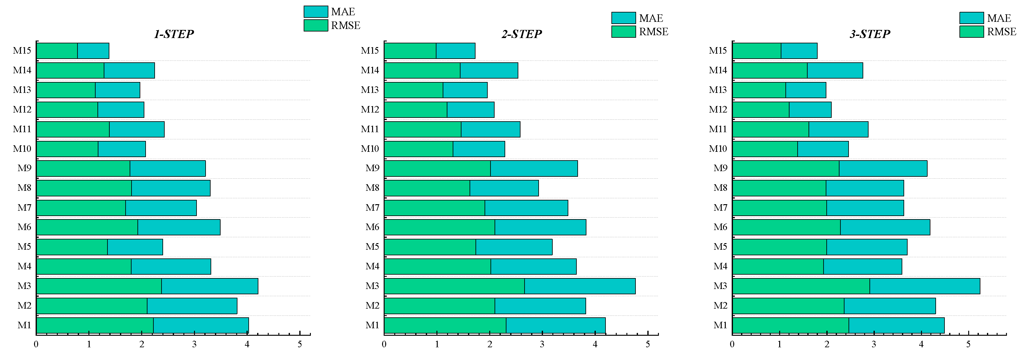
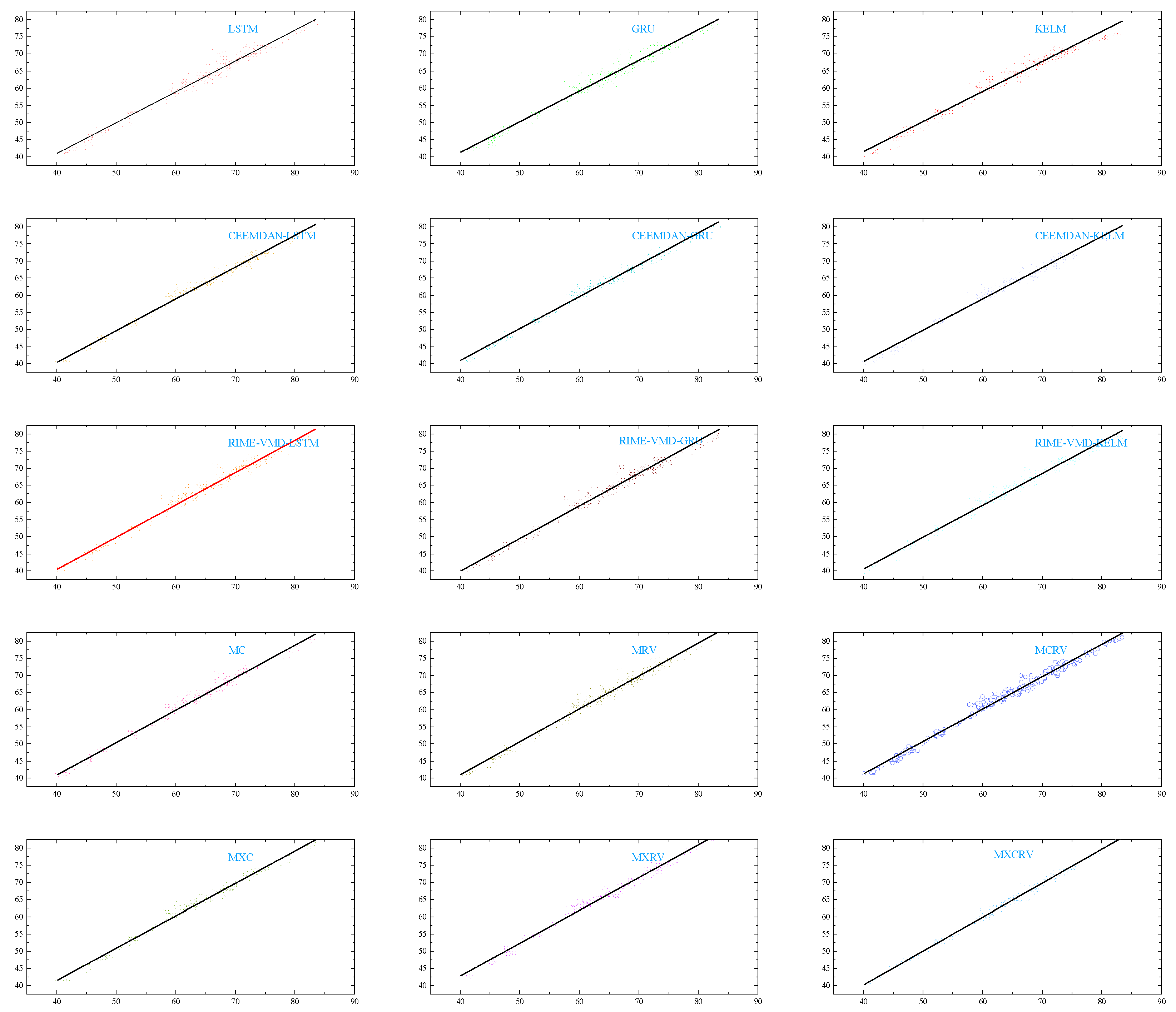
Figure 7.
Forecasting results of 15 models in WTI.
4.2. Brent Crude Oil Futures Price Forecast Results
The radar chart in Figure 8 illustrates the RMSE and MAE of 15 models on the Brent crude oil futures price test set. From Table 5 and Figure 9, it can be observed that CEEMDAN-LSTM and CEEMDAN-KELM exhibit poorer performance compared to LSTM and KELM. However, CEEMDAN-GRU is notably superior to GRU. This may be due to overfitting or improper parameter settings in CEEMDAN-LSTM and CEEMDAN-KELM. Hence, it is evident that a single machine learning model may perform differently on various datasets and may not entirely adapt to different data characteristics.
By employing MOSMA-XGBoost and MOSMA to integrate different machine learning prediction results, this issue can be effectively addressed. For instance, in the one-step-ahead prediction of Brent, the ensemble strategy M11 reduces RMSE, MAE, and MAPE by 15.4%, 18.5%, and 18.0%, respectively, compared to using only decomposition algorithms like M7, M8, and M9. Additionally, the non-linear ensemble model outperforms the linear weighted ensemble model. For instance, in one-step-ahead prediction, M15 decreases RMSE, MAE, and MAPE by 40.1%, 39.1%, and 38.1%, respectively, compared to M12. This highlights the superior performance of non-linear ensemble methods over linear weighted ensemble methods in handling crude oil futures price prediction problems.
Figure 8.
Brent’s RMSE and MAE Radar Charts.
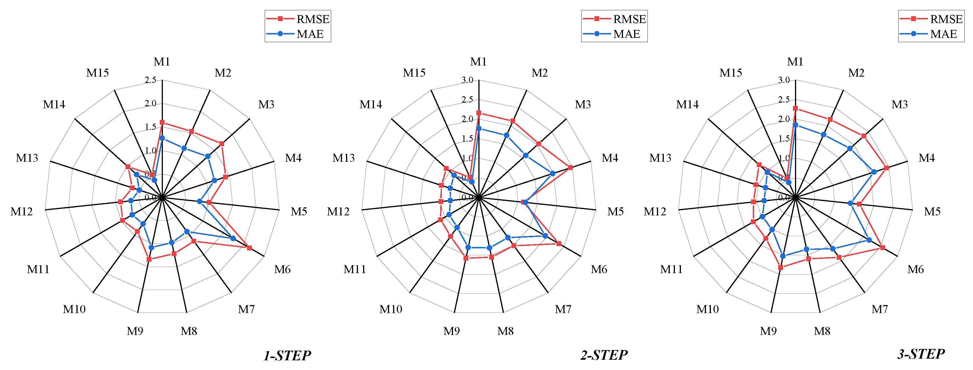
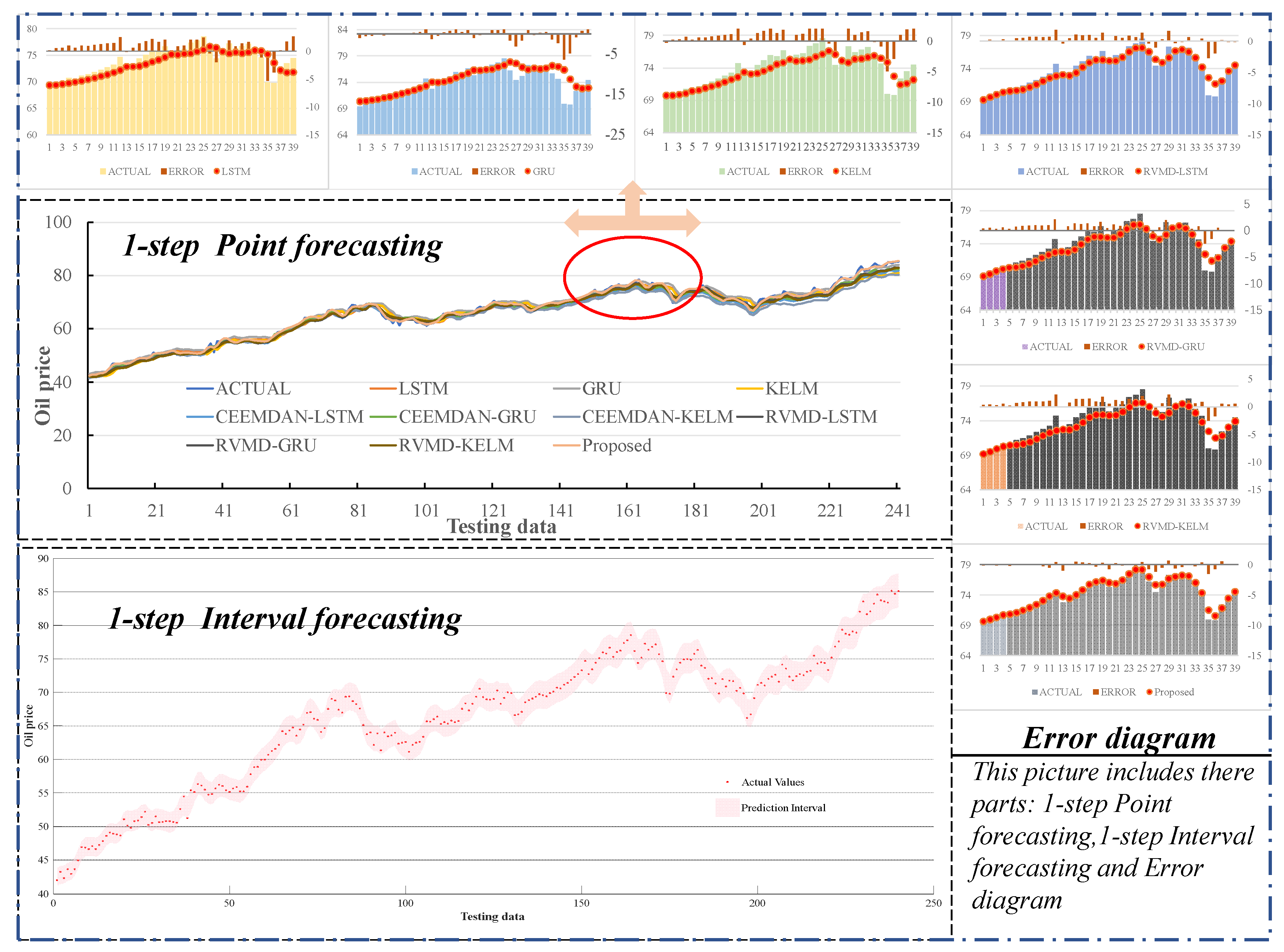
Figure 9.
Brent’s one-step-ahead prediction result graph and error diagram.
4.3. Uncertainty Estimate
Although the MXCRV model has demonstrated good accuracy on the test sets of WTI and Brent crude oil futures prices, the prices of crude oil futures are closely tied to various factors such as global political and economic conditions, leading to significant uncertainty. So Interval estimation results is crucial for risk assessment and uncertainty evaluation. In this study, we utilize the combination of six models’ forecasting results through MOSMA-XGBoost to obtain upper and lower limits of interval prediction. To highlight the superiority of this approach, we refer to it as MXQ and compare it with KDE and Bootstrap. As shown in Table 6, MXQ achieves over 95% Prediction Interval Coverage Probability (PICP) and a PINAW (Prediction Interval Normalized Average Width) lower than 0.1 in multi-step forecasting. Although MXQ’s Coverage Width Coefficient (CWC) is higher than KDE and Bootstrap, the PICP of KDE and Bootstrap is both below 95%, indicating poorer practicality. Therefore, interval prediction based on nonlinear ensemble methods can yield interval estimates with greater practical significance, assisting governments and relevant investors in mitigating potential future risks.
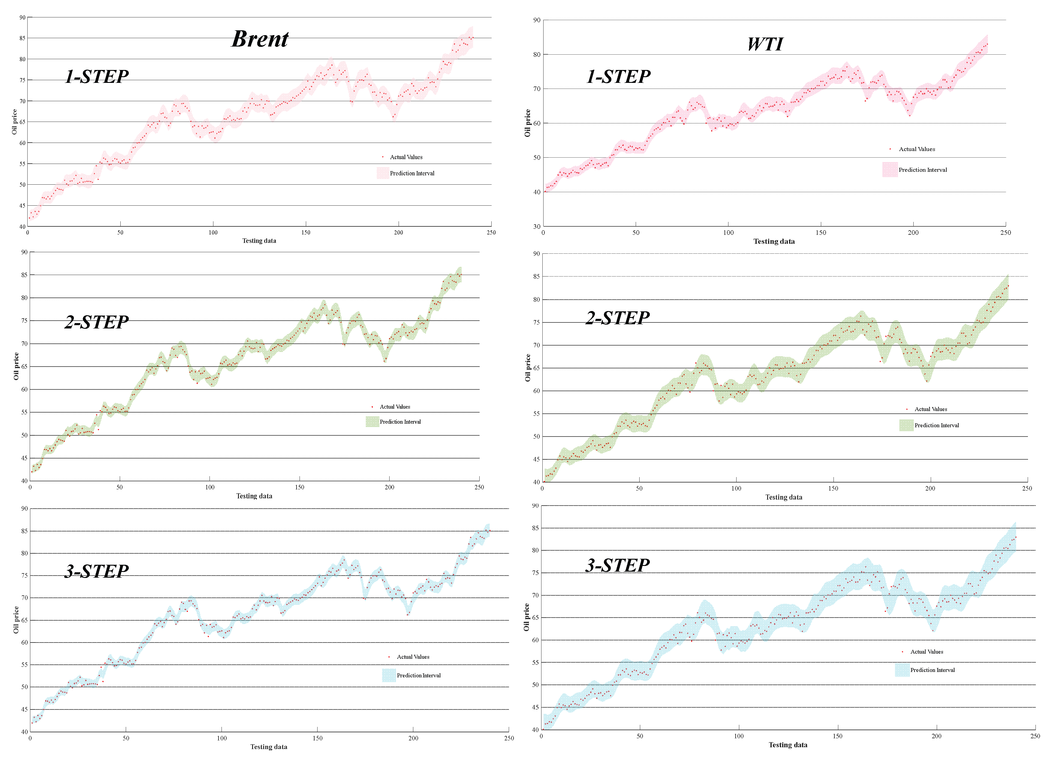
Figure 10.
Range prediction charts for WTI and Brent.
4.4. Analysis of the Validity of the Model
The combination model proposed in this paper achieves better performance than other models in both point prediction and interval prediction, and analyzes its inevitability from the perspective of modeling ideas, mainly including:
(1) The prediction effect of the dual-mode decomposition method is better than that of the single-mode decomposition method, and the reasonable combination of dual-mode decomposition is conducive to improving the prediction accuracy. The multi-scale complementary components brought by different decomposition methods can completely reflect the complex fluctuation characteristics of the original signal, which is conducive to the subsequent model for feature extraction.
(2) The model of the ensemble decomposition algorithm and the ensemble strategy can improve the prediction ability of the model better than the single use of the decomposition algorithm.
(3) The ensemble strategy can overcome the limitations of a single machine learning model and the shortcomings of unimodal decomposition, and jointly harvest the advantages of various predictors and algorithms to jointly improve the prediction accuracy. Besides, nonlinear ensemble performs better than weighted ensemble in modeling accuracy.
(4) Not only can it combine the advantages of various models in point forecasting; but MXQ with nonlinear ensemble can provide more practical PICP and PINAW in interval forecasting compared with KDE and Bootstrap.
4.5. Shortcomings of the Model
Although the MXCRV model has substantially improved in accuracy, we can improve it in the following aspects. (1) Although RIME can effectively select the parameters for VMD decomposition, more advanced optimization algorithms can be used to combine with VMD, in addition to more suitable objective functions for VMD decomposition. (2) From the CEEMDAN-based model, it is known that there are certain problems in the parameter selection of LSTM and KELM, so optimization algorithms can be used to combine with them to further improve the prediction accuracy of the model.
5. Conclusion and Outlook
As an important energy and chemical raw material, the price trend of crude oil has a crucial impact on economic and social development. Aiming at the nonlinear characteristics of crude oil futures price, a new hybrid model for crude oil futures price prediction is proposed and compared with 15 prediction models such as RIME-VMD-GRU, CEEMDAN-LSTM, MCRV and so on. The results show that the model outperforms the other 14 models in all indicators. The main innovations of this study are: (1) the establishment of the model framework of “dual-mode decomposition-multi-learners prediction-nonlinear integration”, which makes the modal decomposition more capable of mining the characteristic information of the price series; (2) the fusion of the prediction results of the six models by using the MOSMA-XGBoost, which can effectively solve the shortcomings of the single-mode decomposition and the problems of the single machine learning model. which effectively solves the shortcomings of single-mode decomposition and the limitations of single machine learning model, and improves the prediction accuracy of the model. (3) Interval estimation of point prediction results using MXQ can provide high PICP and narrow PINAW.
Author Contributions
Luming Zhou: Software, Writing original draft. Kai Wu: Investigation. Yunlong Zhao: Data curation.
Funding
This research received no external funding
Data Availability Statement
Data will be made available on request.
Acknowledgments
During the preparation of this manuscript, the author(s) used deepseek for the purposes of translate. The authors have reviewed and edited the output and take full responsibility for the content of this publication.
Conflicts of Interest
The authors declare no conflicts of interest.
References
- Ambach, D. & O. Ambach. 2018. Forecasting the Oil Price with a Periodic Regression ARFIMA-GARCH Process. In 2018 IEEE Second International Conference on Data Stream Mining & Processing (DSMP), 212-217.
- Baumeister, C. & L. Kilian (2012) Real-Time Forecasts of the Real Price of Oil. Journal of Business & Economic Statistics, 30, 326-336. [CrossRef]
- Berrisch, J., S. Pappert, F. Ziel & A. Arsova (2023) Modeling volatility and dependence of European carbon and energy prices. Finance Research Letters, 52, 103503. [CrossRef]
- Bi, g., x. Zhao, l. Li, s. Chen & c. Chen (2023) Short-term wind speed prediction model with dual-mode decomposition CNN-LSTM integration. Journal of Solar Energy, 44, 191-197.
- Chen, Y., J. Lu & M. Ma (2022) How Does Oil Future Price Imply Bunker Price—Cointegration and Prediction Analysis. Energies, 15. [CrossRef]
- Dai, Z., J. Kang & Y. Hu (2021) Efficient predictability of oil price: The role of number of IPOs and U.S. dollar index. Resources Policy, 74, 102297. [CrossRef]
- Drachal, K. (2021) Forecasting crude oil real prices with averaging time-varying VAR models. Resources Policy, 74, 102244. [CrossRef]
- Gong, X., K. Guan, L. Chen, T. Liu & C. Fu (2021) What drives oil prices? — A Markov switching VAR approach. Resources Policy, 74, 102316. [CrossRef]
- Hao, J., Q. Feng, J. Yuan, X. Sun & J. Li (2022) A dynamic ensemble learning with multi-objective optimization for oil prices prediction. Resources Policy, 79, 102956. [CrossRef]
- Hochreiter, S. & J. Schmidhuber (1997) Long Short-Term Memory. Neural Computation, 9, 1735-1780.
- Jovanovic, L., D. Jovanovic, N. Bacanin, A. Jovancai Stakic, M. Antonijevic, H. Magd, R. Thirumalaisamy & M. Zivkovic (2022) Multi-Step Crude Oil Price Prediction Based on LSTM Approach Tuned by Salp Swarm Algorithm with Disputation Operator. Sustainability, 14. [CrossRef]
- Lin, Y., K. Chen, X. Zhang, B. Tan & Q. Lu (2022) Forecasting crude oil futures prices using BiLSTM-Attention-CNN model with Wavelet transform. Applied Soft Computing, 130, 109723. [CrossRef]
- Lux, T., M. Segnon & R. Gupta (2016) Forecasting crude oil price volatility and value-at-risk: Evidence from historical and recent data. Energy Economics, 56, 117-133. [CrossRef]
- Mo, Z. & H. Tao. 2016. A Model of Oil Price Forecasting Based on Autoregressive and Moving Average. In 2016 International Conference on Robots & Intelligent System (ICRIS), 22-25.
- Premkumar, M., P. Jangir, R. Sowmya, H. H. Alhelou, A. A. Heidari & H. Chen (2021) MOSMA: Multi-Objective Slime Mould Algorithm Based on Elitist Non-Dominated Sorting. IEEE Access, 9, 3229-3248. [CrossRef]
- Torres, M. E., M. A. Colominas, G. Schlotthauer, P. Flandrin & Ieee. 2011. A COMPLETE ENSEMBLE EMPIRICAL MODE DECOMPOSITION WITH ADAPTIVE NOISE. In 2011 IEEE INTERNATIONAL CONFERENCE ON ACOUSTICS, SPEECH, AND SIGNAL PROCESSING, 4144-4147.
- Wang, D. & T. Fang (2022) Forecasting Crude Oil Prices with a WT-FNN Model. Energies, 15. [CrossRef]
- Wang, J., T. Niu, P. Du & W. Yang (2020) Ensemble probabilistic prediction approach for modeling uncertainty in crude oil price. Applied Soft Computing, 95, 106509. [CrossRef]
- Wang, L., Y. Xia & Y. Lu (2022) A Novel Forecasting Approach by the GA-SVR-GRNN Hybrid Deep Learning Algorithm for Oil Future Prices. Computational Intelligence and Neuroscience, 2022, 4952215. [CrossRef]
- Wu, C., J. Wang & Y. Hao (2022) Deterministic and uncertainty crude oil price forecasting based on outlier detection and modified multi-objective optimization algorithm. Resources Policy, 77, 102780. [CrossRef]
- Wu, J., J. Dong, Z. Wang, Y. Hu & W. Dou (2023) A novel hybrid model based on deep learning and error correction for crude oil futures prices forecast. Resources Policy, 83, 103602. [CrossRef]
- Wu, L., C. Kong, X. Hao & W. Chen (2020) A Short-Term Load Forecasting Method Based on GRU-CNN Hybrid Neural Network Model. Mathematical Problems in Engineering, 2020, 1428104. [CrossRef]
- Yang, H., Y. Zhang & F. Jiang. 2019. Crude Oil Prices Forecast Based on EMD and BP Neural Network. In 2019 Chinese Control Conference (CCC), 8944-8949.
- Yang, W., M. Hao & Y. Hao (2023) Innovative ensemble system based on mixed frequency modeling for wind speed point and interval forecasting. Information Sciences, 622, 560-586. [CrossRef]
- Yin, L. & Q. Yang (2016) Predicting the oil prices: Do technical indicators help? Energy Economics, 56, 338-350. [CrossRef]
- Zhang, S., J. Luo, S. Wang & F. Liu (2023) Oil price forecasting: A hybrid GRU neural network based on decomposition–reconstruction methods. Expert Systems with Applications, 218, 119617. [CrossRef]
- Zhao, Y., W. Zhang, X. Gong & C. Wang (2021) A novel method for online real-time forecasting of crude oil price. Applied Energy, 303, 117588. [CrossRef]
Figure 4.
Results of the RIME-VMD decomposition of Brent.
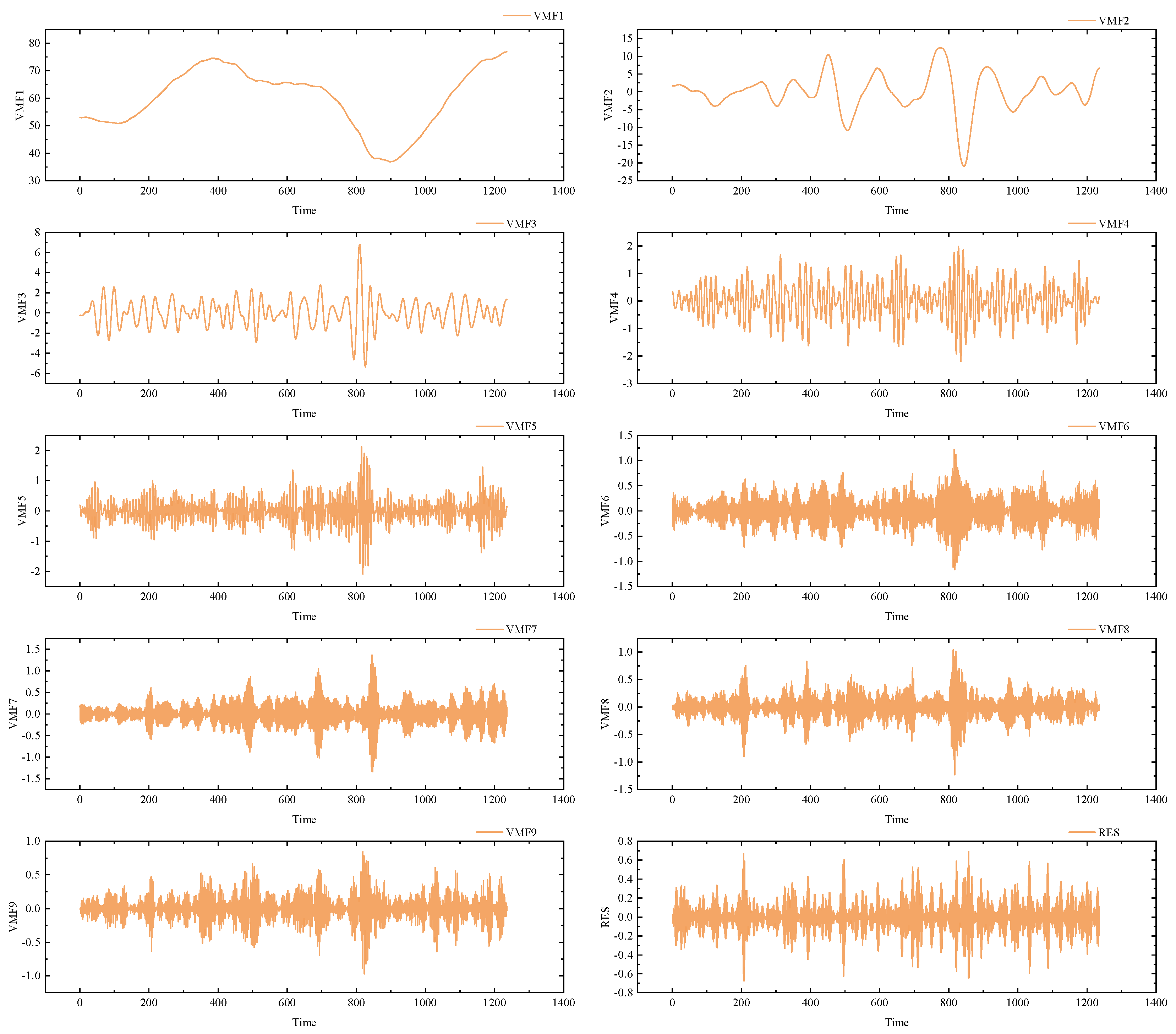
Figure 5.
Results of the CEEMDAN decomposition of Brent.
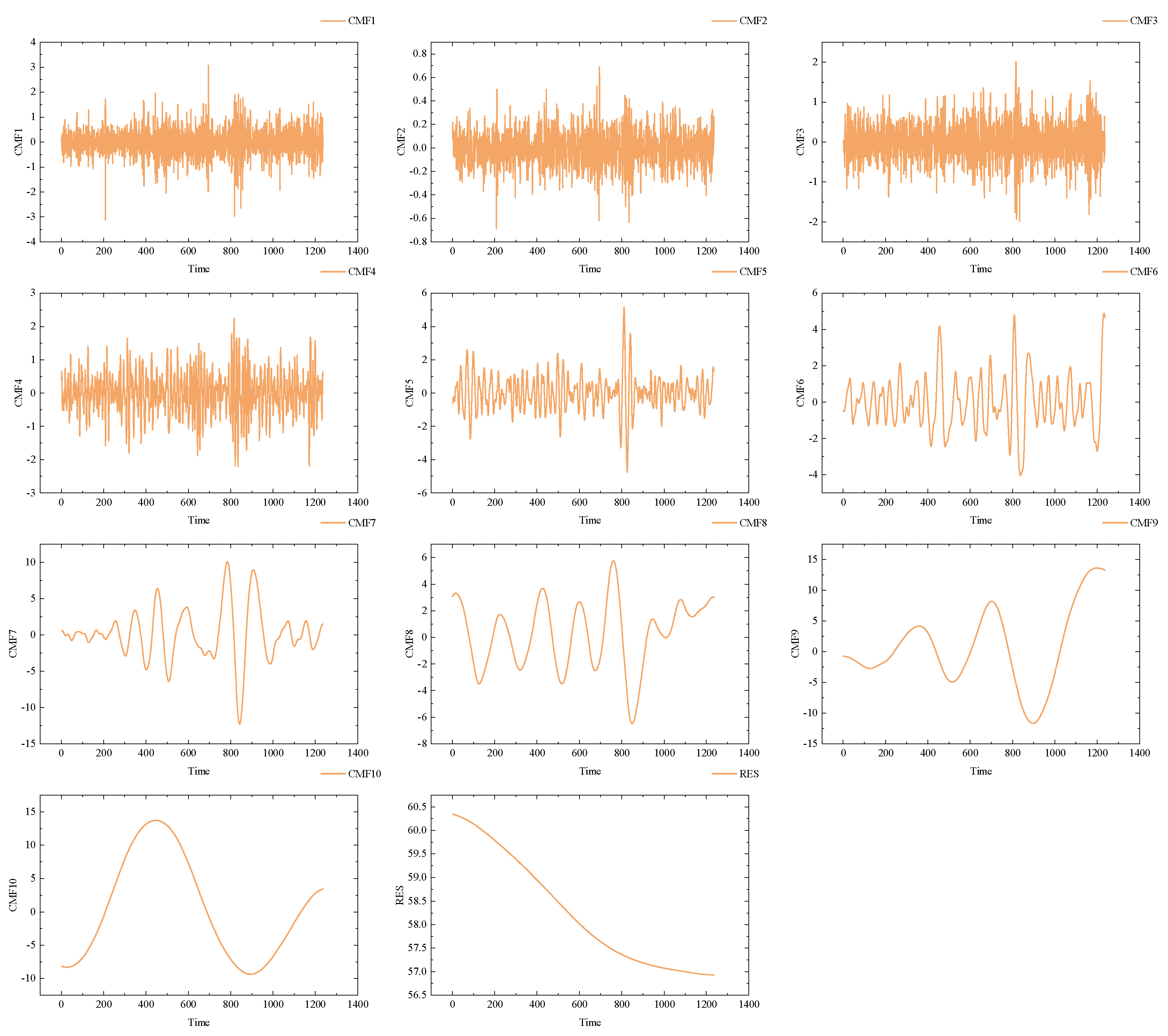
Table 6.
Interval projection indicator values.
| MSQ | KDE | Bootstrap | ||||||||
| PICP | PINAW | CWC | PICP | PINAW | CWC | PICP | PINAW | CWC | ||
| 1 | 100% | 0.0928 | 0.5568 | 91.67% | 0.0429 | 0.2574 | 85.42% | 0.043 | 0.358 | |
| Brent | 2 | 97.50% | 0.0606 | 0.3636 | 90.83% | 0.0447 | 90.83% | 86.66% | 0.0433 | 0.3598 |
| 3 | 95.83% | 0.0523 | 0.3138 | 92.08% | 0.0433 | 92.08% | 85.83% | 0.0435 | 0.361 | |
| 1 | 98.75% | 0.0914 | 0.5484 | 85.42% | 0.0542 | 0.4252 | 85.00% | 0.0531 | 0.4186 | |
| WTI | 2 | 97.48% | 0.0996 | 0.5976 | 85.42% | 0.0648 | 0.4888 | 85.42% | 0.0874 | 0.6244 |
| 3 | 96.67% | 0.1100 | 0.6600 | 85.00% | 0.0681 | 0.5086 | 86.25% | 0.0868 | 0.6208 |
Disclaimer/Publisher’s Note: The statements, opinions and data contained in all publications are solely those of the individual author(s) and contributor(s) and not of MDPI and/or the editor(s). MDPI and/or the editor(s) disclaim responsibility for any injury to people or property resulting from any ideas, methods, instructions or products referred to in the content. |
© 2025 by the authors. Licensee MDPI, Basel, Switzerland. This article is an open access article distributed under the terms and conditions of the Creative Commons Attribution (CC BY) license (https://creativecommons.org/licenses/by/4.0/).
Copyright: This open access article is published under a Creative Commons CC BY 4.0 license, which permit the free download, distribution, and reuse, provided that the author and preprint are cited in any reuse.


