Submitted:
18 August 2025
Posted:
19 August 2025
You are already at the latest version
Abstract
To address the time-series characteristics of financial data, this paper proposes a data preprocessing method based on Sliding Window–Variational Mode Decomposition (SW-VMD). The method decomposes and reconstructs stock index closing prices and return time series, transforming nonlinear and nonstationary sequences into linear and stationary data. The processed data is then used as input for a Long Short-Term Memory (LSTM) neural network to predict future stock index closing prices and returns. Empirical analysis adopts trend accuracy as the evaluation metric to reflect the model's capability in forecasting the upward or downward trends of the next day's closing price and return. Results indicate that, compared to models without data decomposition, the LSTM model enhanced with SW-VMD shows significant improvements in trend prediction accuracy.
Keywords:
sliding window
; variational mode decomposition
; long short-term memory neural network
; financial time series forecasting
1. Introduction
Financial time series forecasting refers to the use of historical data to build time series or other econometric models to predict key financial indicators such as prices, indices, returns, and volatility. Accurate forecasting of financial time series data enhances the understanding of market volatility, assists government agencies in risk control, and helps investors formulate more rational investment strategies using market fluctuation information.
Classical financial time series prediction methods primarily employ statistical models such as ARCH (Autoregressive Conditional Heteroskedasticity Model) and GARCH (Generalized ARCH), as well as their improved versions. These models describe features like heteroskedasticity and volatility clustering in financial markets [1,2].
With the advent of the deep learning era in the 21st century, numerous classic neural network models have emerged, such as Convolutional Neural Networks (CNN), Deep Belief Networks (DBN), Autoencoders (AE), and Recurrent Neural Networks (RNN). Among them, Long Short-Term Memory (LSTM) networks are particularly effective for processing sequential data. LSTM, proposed by Sepp Hochreiter and Jürgen Schmidhuber in 1997 [3], is a type of RNN that effectively captures long-term dependencies in time series by retaining relevant historical information within neurons.
LSTM has been widely applied in financial time series forecasting. For example, Jin Xuejun (2016) used LSTM to study whether China’s inflation level was affected by the expansionary monetary policy of the United States. He compared the results with a Value at Risk (VAR) model and concluded that LSTM outperformed VAR in economic analysis [4].
Xie Heliang et al. (2018) constructed an LSTM-based option pricing model and conducted empirical analysis using 50ETF call and put options. Their results showed that the LSTM model provided higher pricing accuracy than the classic Black-Scholes Monte Carlo method [5].
Li Ying and Wang Lulu (2020) proposed a GA-LSTM model, which integrates Genetic Algorithms to optimize LSTM parameters. They applied this to model complex, nonlinear time series data in the futures market and achieved improved prediction accuracy [6].
Chen Qiqi (2020) utilized CNNs to extract spatial structural features from data, followed by LSTM for sequential feature extraction. This CNN-LSTM hybrid model was shown to effectively predict short-term intraday stock highs [7].
Properly preprocessed datasets significantly enhance model performance. Effective decomposition techniques for time series include Empirical Mode Decomposition (EMD) [8] and Variational Mode Decomposition (VMD) [9], originally proposed for noise reduction in engineering signal processing. These methods have since been applied to financial data such as crude oil [10] and gold prices [11].
VMD is a recently proposed adaptive signal decomposition method based on variational principles. It formulates an optimization problem that minimizes the sum of bandwidths of each mode, decomposing the signal into multiple quasi-orthogonal intrinsic mode functions (IMFs) with reduced noise and redundancy.
Due to the nonlinear and nonstationary characteristics of financial time series data, direct application of historical closing prices and returns to LSTM models often results in lagged predictions. This compromises the accuracy of trend forecasts. To address this, we propose a Sliding Window Variational Mode Decomposition (SW-VMD) method to process Chinese stock index data. After extracting key features, LSTM networks are used to predict price and return trends. Comparative experiments are designed to validate the model’s effectiveness.
2. Related Work
Recent developments in financial time-series forecasting have significantly benefited from advanced deep learning models. Models built on convolutional neural networks (CNNs) have proven effective in extracting spatial features from stock volatility data, enhancing predictive accuracy in financial contexts [12]. Meanwhile, reinforcement learning methods have been successfully adapted for financial decision-making and scheduling, leveraging multi-agent strategies to navigate complex market dynamics [13]. Efforts to combine multimodal data sources through feedforward networks have also demonstrated promising results in improving the robustness of stock prediction models [14].
In the domain of financial text analysis, one-dimensional CNNs have enabled high-precision risk classification and auditing capabilities, underscoring the versatility of CNN-based architectures [15]. Reinforcement learning continues to show potential for nonlinear and dynamic risk control in volatile financial markets through nested temporal frameworks [16]. Enhancements to reinforcement learning algorithms, such as those based on the A3C model, have further contributed to more accurate market turbulence prediction and proactive risk management [17].
Outside of core financial forecasting, diffusion models have been introduced for interface generation, which—while outside traditional financial domains—offer insights into generative modeling applicable to data synthesis and scenario simulations [18]. Transfer learning methods for large language models have further introduced dynamic fine-tuning strategies that can support robust few-shot learning, critical for domains with sparse financial event data [19].
Graph-based learning has also been employed to detect transaction fraud by modeling network structures, supporting the idea of relational modeling in financial data streams [20]. In portfolio optimization, reinforcement learning methods such as QTRAN have been applied to dynamically allocate resources, providing a theoretical basis for strategic financial positioning [21].
Anomaly detection techniques based on global temporal attention and transformer models have emerged in video and sequential data, which can be translated into high-frequency trading data analysis [22]. Ensemble and data balancing methods have enhanced classification tasks such as credit card fraud detection [23], while heterogeneous graph attention networks have enabled deep fraud analytics in heterogeneous financial environments [24].
Probabilistic graphical models and variational inference have addressed class imbalance problems often found in financial classification datasets [25]. Advances in BERT-based compliance analysis have improved audit automation through contextual understanding [26], and deep anomaly detection systems have demonstrated efficacy in uncovering irregularities in high-frequency trading scenarios [27].
Causal representation learning has been proposed for market return forecasting, revealing the impact of hidden variables on prediction tasks [28]. Temporal graph learning frameworks and hybrid LSTM-Copula methods have contributed significantly to modeling user behavior and portfolio risk across evolving markets [29,30]. BiLSTM-CRF models, originally used in social text segmentation, offer transferable techniques for boundary detection in labeled financial sequences [31].
Further research on causal inference for return prediction across markets has refined the cross-domain forecasting capability of financial models [32], while multi-task learning architectures have been employed for macroeconomic forecasting, reinforcing the importance of domain fusion [33]. Decision-making dynamics in audit workflows have also been enhanced through deep Q-learning frameworks [34].
3. LSTM Neural Network Based on SW-VMD Data Decomposition
We first construct the sliding window VMD data decomposition algorithm and the LSTM network, then integrate the preprocessed data with the neural network to build separate models for stock index closing prices and returns.
3.1. Sliding Window–Variational Mode Decomposition Algorithm
The core concept of the Variational Mode Decomposition (VMD) algorithm is to transform the decomposition of the original time series into a constrained variational optimization problem. Under the condition that the sum of all intrinsic mode functions (IMFs) and the residual equals the original signal, the algorithm aims to minimize the estimated bandwidth of each mode. Based on this condition, the center frequency and bandwidth of each decomposed mode are determined, enabling adaptive frequency-domain partitioning and effective separation of the signal components. Through iterative optimization, the center frequencies and mode functions are continuously updated until multiple IMFs are obtained. The number of IMFs is predefined manually.
For the financial time series data in this study, each VMD decomposition result is influenced by the entire original signal. This means that if the entire time series is decomposed at once, the decomposition result at the current time point will contain information from future data. Consequently, this prevents valid predictive analysis based on current data decomposition.
To address this, we propose a sliding window-based VMD decomposition strategy. Specifically, a dataset of 32 days is treated as a window, and the decomposition is performed in a progressive manner. The detailed process is as follows: the data from Day 1 to Day 32 is decomposed using VMD, and the decomposition result of Day 32 is taken as the first input for the model to predict the closing price and return of Day 33. This process continues iteratively—i.e., the decomposition of data from Day to Day n yields the decomposition result of Day n, which serves as the input to the model to predict the day’s results.
The decomposition data construction process is illustrated in Figure 1.
In Figure 1, VMD_i () denotes the set of data undergoing VMD decomposition. VMD_i_j () represents the decomposed result of the day from the VMD operation. VMD_i indicates the input variable for the model, corresponding to the final item in the VMD result of the decomposition. That is, VMD32 = VMD_1_32, VMD33 = VMD_2_33, VMD34 = VMD_3_34, and so on until VMD_n = VMD_(n).
3.2. LSTM Network Structure
The Long Short-Term Memory (LSTM) neural network consists of three main components: an input layer, an output layer, and hidden layers. The number of hidden layers and the number of neurons in each layer determine the network’s depth and complexity. Analogous to biological neural networks, neurons are the smallest computational units capable of processing information. LSTM uses neurons to selectively allow sequence information to influence the network state at each training step. Activation functions such as tanh, sigmoid, and ReLU are used to output values between 0 and 1 as gates, which determine how much of the current input can pass through these "gates."
A "layer" refers to a group of neurons, and the overall network is formed by connecting these layers in a structured manner. The LSTM algorithm includes two processes: forward propagation and backpropagation. During forward propagation, information is processed through the forget gate, input gate, and output gate in order. In backpropagation, the chain rule is used to compute gradients of weights and biases in each neuron, which are iteratively updated using optimization algorithms until a suitable neural network model is trained.
Figure 2 shows the structure of an LSTM unit.
As illustrated in Figure 2, the LSTM network not only extracts useful information from the current data state in a sequence but also retains long-term dependencies from earlier computation steps that are far from the current state. This makes LSTM one of the ideal tools for solving time-series problems.
In summary, the specific algorithmic process of the LSTM time-series forecasting model based on SW-VMD data decomposition is as follows:
- Step 1: Apply Sliding Window–Variational Mode Decomposition to stock index closing price and return sequences of length n, generating input data of length with m intrinsic mode functions (IMFs).
- Step 2: Split the data into training, validation, and testing sets. The validation set covers 30 days, and the testing set spans 60 days.
- Step 3: During training, introduce the validation set after 1000 training steps. Perform validation every 30 steps and save the model that performs best on the validation set.
- Step 4: Input the test set into the best-performing saved model to predict stock index closing prices and returns. Evaluate and compare the effects of different models and datasets on prediction performance.
4. Empirical Analysis
Due to their strong representativeness in the stock market and relatively stable investment profile, this study selects the Shanghai Composite Index and the CSI 300 Index. Historical information prior to each time point is used to build LSTM neural network models to predict the next day’s stock index closing price and return trends.
To assess the effectiveness of the algorithm on datasets with different volatilities, both the relatively stable closing price and the highly volatile return series are decomposed for model construction. Models using raw data and those using SW-VMD decomposed data are compared to evaluate the impact of decomposition on model prediction performance.
The logarithmic return is calculated using adjacent closing prices as follows:
Based on the return sequence, the price trend is defined as:
The input variables for the LSTM model without data decomposition include closing price, highest price, lowest price, previous closing price, trading volume, and return. For the SW-VMD-based model, the number of intrinsic mode functions (IMFs) is set to 6, and both closing price and return data are decomposed per the process in Figure 1.
4.1. Stationarity and Memory Property Testing
ADF (Augmented Dickey-Fuller) tests are performed to assess the stationarity of the time series. A series is considered stationary if the test statistic is less than the critical values at 1%, 5%, or 10% levels. Table 1 shows the ADF results.
The Hurst exponent is then used to evaluate the memory properties of the time series before model training. Table 2 displays the results.
The results show that the return sequences fall in the range [0.45, 0.5], indicating long memory with weak anti-persistence. Closing price sequences have Hurst values above 0.5, indicating strong persistence—when prices rise, they tend to keep rising, and vice versa.
4.2. Data Processing and Decomposition
The SW-VMD algorithm is applied to decompose the closing price and return series of both indices into six IMFs. An example of the VMD decomposition for the CSI 300 closing price is shown in Figure 3.
4.3. Prediction Results and Analysis
The LSTM is implemented using the TensorFlow framework. Data is normalized using Z-score standardization. The model is configured with 3 hidden layers, each containing 128 neurons. Batch size is set to 256, time step to 1, and number of iterations to 5000. Dropout rate is 0.1 to avoid overfitting. Both L1 and L2 regularizations are applied with parameters 0.01.
A fixed step decay learning rate is used, starting at 0.0015 and decaying by 97.5% every 50 steps. The Adam optimizer is employed. The training loss function is defined by the mean squared error (MSE):
The total data lengths are 7207 (SSE) and 3264 (CSI 300). After applying a 32-day sliding window, usable lengths are 7176 and 3233. The last 60 entries are used as the test set, and the previous 30 as the validation set.
4.4. Validation and Performance Evaluation
Figure 6 and Figure 7 show the trend prediction accuracy on the validation set. In 180 validations, the SW-VMD-enhanced model outperformed the raw model 158 and 120 times for SSE and CSI 300 price prediction (87.78% and 66.67%). For returns, SW-VMD outperformed in 148 and 173 cases (82.22% and 96.11%).
Overall, SW-VMD improves trend accuracy by 5.28% for price and 12.65% for return. The method is especially effective on more volatile time series.
5. Conclusion
This paper proposes an optimized forecasting approach for financial time series based on the Sliding Window–Variational Mode Decomposition (SW-VMD) and LSTM neural network. Since VMD extracts intrinsic mode functions from an entire dataset, a sliding window approach ensures proper use of historical data without leaking future information.
The decomposed data not only exhibit linearity and stationarity but also enhance feature extraction and reuse. Deep learning models built on these inputs show superior performance compared to models using raw data.
Empirical results on two Chinese stock indices demonstrate that SW-VMD improves model convergence and predictive accuracy, especially on volatile return sequences. This confirms the proposed method’s advantage in forecasting high-volatility financial time series.
References
- Engle RF. Autoregressive conditional heteroscedasticity with estimates of the variance of United Kingdom inflation. Econometrica, 1982, 50(4): 987. [CrossRef]
- Bollerslev T. Generalized autoregressive conditional heteroskedasticity. J Econometrics, 1986, 31(3): 307–327. [CrossRef]
- Hochreiter S, Schmidhuber J. Long short-term memory. Neural Computation, 1997, 9(8): 1735–1780.
- Li Y, Ma W. Applications of artificial neural networks in financial economics: a survey. In: 2010 Int Symp on Computational Intelligence and Design, IEEE, 2010: 211–214.
- Hutchinson JM, Lo AW, Poggio T. A nonparametric approach to pricing and hedging derivative securities via learning networks. J Finance, 1994, 49(3): 851–889.
- Nelson DM, Pereira AC, De Oliveira RA. Stock market’s price movement prediction with LSTM neural networks. In: 2017 Int Joint Conf on Neural Networks (IJCNN), IEEE, 2017: 1419–1426.
- Chen K, Zhou Y, Dai F. A LSTM-based method for stock returns prediction: A case study of China stock market. In: 2015 IEEE Int Conf on Big Data, IEEE, 2015: 2823–2824.
- Huang NE, Shen Z, Long SR, et al. The empirical mode decomposition and the Hilbert spectrum for nonlinear and non-stationary time series analysis. Proc Royal Soc London A, 1998, 454(1971): 903–995.
- Dragomiretskiy K, Zosso D. Variational mode decomposition. IEEE Trans Signal Process, 2014, 62(3): 531–544.
- Jianwei E, Bao YL, Ye JM. Crude oil price analysis and forecasting based on variational mode decomposition and independent component analysis. Physica A, 2017, 484: 412–427. [CrossRef]
- Jianwei E, Shenggang L, Ye JM. A new approach to gold price analysis based on variational mode decomposition and independent component analysis. Acta Phys Pol B, 2017, 48(11): 2093. [CrossRef]
- Liu J. Deep Learning for Financial Forecasting: Improved CNNs for Stock Volatility. J Comput Sci Software Appl, 2025, 5(2).
- Wang B. Topology-aware decision making in distributed scheduling via multi-agent reinforcement learning. Trans Comput Sci Methods, 2025, 5(4).
- Wang Y. Stock Prediction with Improved Feedforward Neural Networks and Multimodal Fusion. J Comput Technol Softw, 2025, 4(1).
- Du X. Financial Text Analysis Using 1D-CNN: Risk Classification and Auditing Support. arXiv:2503.02124, 2025.
- Yao Y. Time-Series Nested Reinforcement Learning for Dynamic Risk Control in Nonlinear Financial Markets. Trans Comput Sci Methods, 2025, 5(1).
- Liu J, Gu X, Feng H, et al. Market Turbulence Prediction and Risk Control with Improved A3C Reinforcement Learning. In: 2025 8th Int Conf on Advanced Algorithms and Control Engineering (ICAACE), IEEE, 2025: 2634–2638.
- Duan Y, Yang L, Zhang T, et al. Automated UI Interface Generation via Diffusion Models. In: 2025 4th Int Symp on Computer Applications and Information Technology (ISCAIT), IEEE, 2025: 780–783.
- Cai G, Kai A, Guo F. Dynamic and Low-Rank Fine-Tuning of Large Language Models for Robust Few-Shot Learning. Trans Comput Sci Methods, 2025, 5(4).
- Guo X, Wu Y, Xu W, et al. Graph-Based Representation Learning for Identifying Fraud in Transaction Networks. In: 2025 IEEE 6th Int Seminar on AI, Networking and Information Technology (AINIT), IEEE, 2025: 1598–1602.
- Xu Z, Bao Q, Wang Y, et al. Reinforcement Learning in Finance: QTRAN for Portfolio Optimization. J Comput Technol Softw, 2025, 4(3).
- Liu J. Global Temporal Attention-Driven Transformer Model for Video Anomaly Detection. In: 2025 5th Int Conf on AI and Industrial Technology Applications (AIITA), IEEE, 2025: 1909–1913.
- Wang Y. A Data Balancing and Ensemble Learning Approach for Credit Card Fraud Detection. In: 2025 4th Int Symp on Computer Applications and Information Technology (ISCAIT), IEEE, 2025: 386–390.
- Sha Q, Tang T, Du X, et al. Detecting Credit Card Fraud via Heterogeneous Graph Neural Networks with Graph Attention. arXiv:2504.08183, 2025.
- Lou Y, Liu J, Sheng Y, et al. Addressing Class Imbalance with Probabilistic Graphical Models and Variational Inference. In: 2025 5th Int Conf on AI and Industrial Technology Applications (AIITA), IEEE, 2025: 1238–1242.
- Xu Z, Sheng Y, Bao Q, et al. BERT-Based Automatic Audit Report Generation and Compliance Analysis. In: 2025 5th Int Conf on AI and Industrial Technology Applications (AIITA), IEEE, 2025: 1233–1237.
- Bao Q, Wang J, Gong H, et al. A Deep Learning Approach to Anomaly Detection in High-Frequency Trading Data. In: 2025 4th Int Symp on Computer Applications and Information Technology (ISCAIT), IEEE, 2025: 287–291.
- Sheng Y. Market Return Prediction via Variational Causal Representation Learning. J Comput Technol Softw, 2024, 3(8).
- Liu X, Xu Q, Ma K, et al. Temporal Graph Representation Learning for Evolving User Behavior in Transactional Networks. Unpublished or forthcoming, 2025.
- Xu W, Ma K, Wu Y, et al. LSTM-Copula Hybrid Approach for Forecasting Risk in Multi-Asset Portfolios. Unpublished or forthcoming, 2025.
- Zhao Y, Zhang W, Cheng Y, et al. Entity Boundary Detection in Social Texts Using BiLSTM-CRF with Integrated Social Features. Unpublished or forthcoming, 2025.
- Wang Y, Sha Q, Feng H, et al. Target-Oriented Causal Representation Learning for Robust Cross-Market Return Prediction. J Comput Sci Software Appl, 2025, 5(5).
- Lin Y, Xue P. Multi-Task Learning for Macroeconomic Forecasting Based on Cross-Domain Data Fusion. J Comput Technol Softw, 2025, 4(6).
- Liu Z, Zhang Z. Modeling Audit Workflow Dynamics with Deep Q-Learning for Intelligent Decision-Making. Trans Comput Sci Methods, 2024, 4(12).
- Su X. Predictive Modeling of Volatility Using Generative Time-Aware Diffusion Frameworks. J Comput Technol Softw, 2025, 4(5).
- Zhang W, Xu Z, Tian Y, et al. Unified Instruction Encoding and Gradient Coordination for Multi-Task Language Models. Unpublished or forthcoming, 2025.
Figure 1.
Data Construction Process Based on Sliding Window and VMD
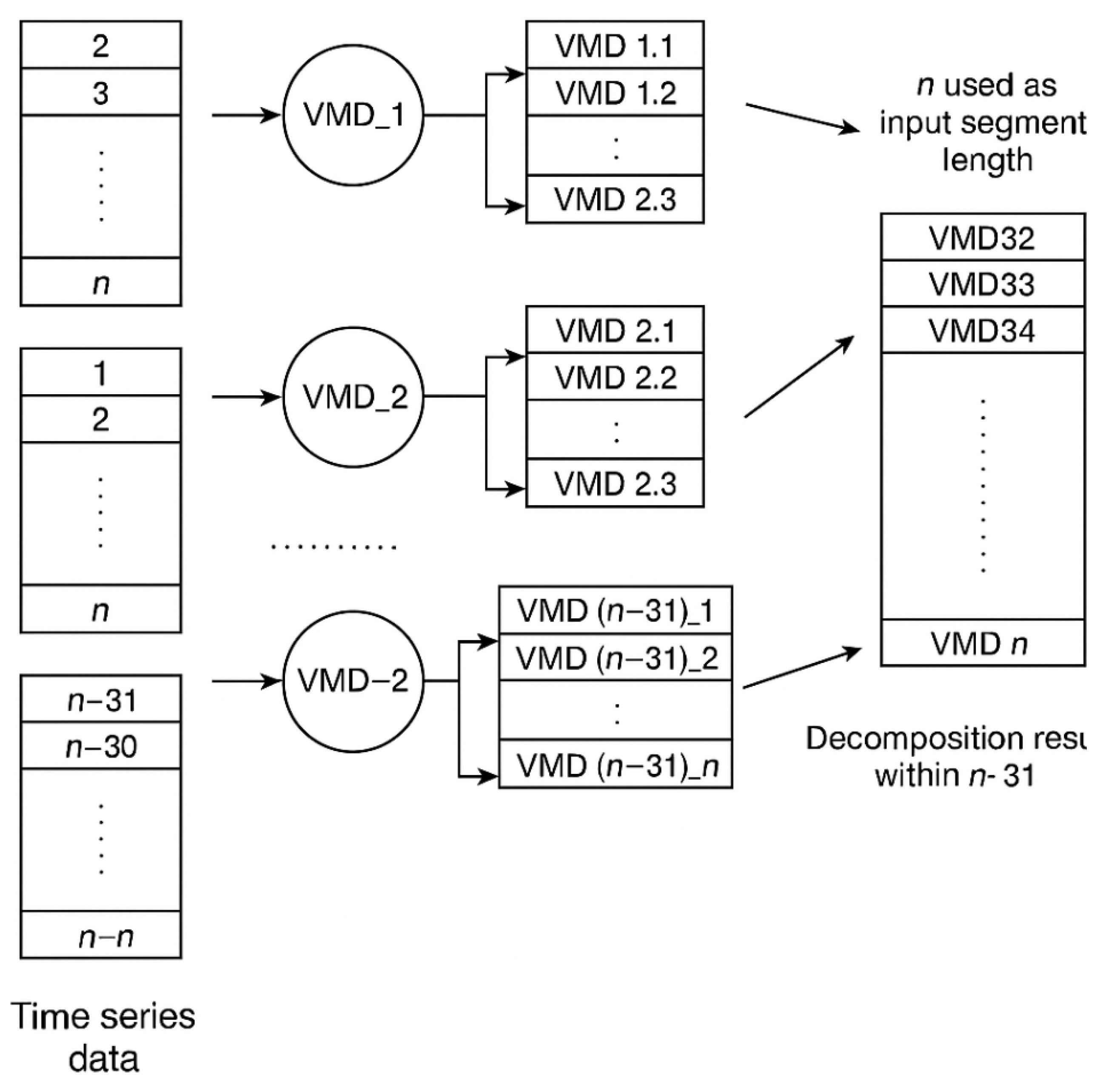
Figure 2.
Shows the structure of an LSTM unit
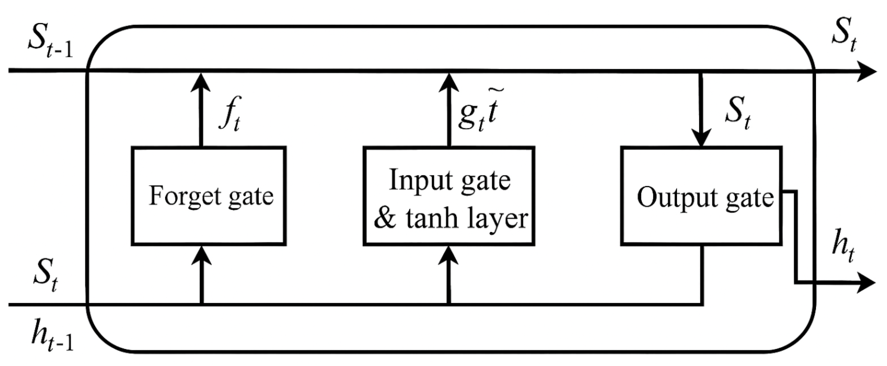
Figure 3.
VMD Decomposition of CSI 300 Closing Prices
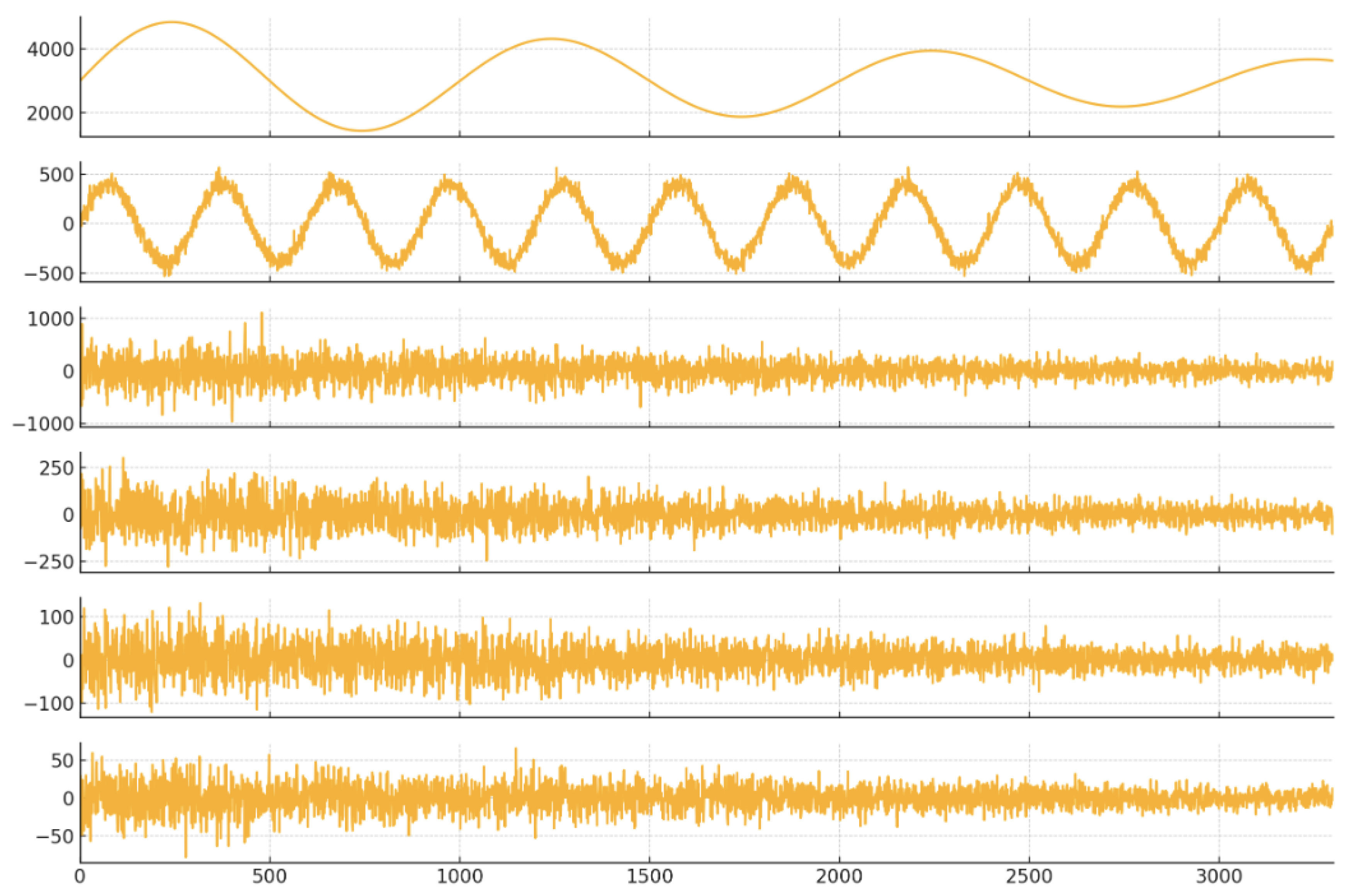
Figure 4.
Comparison of Training Loss for Price Prediction Models on SSE Index
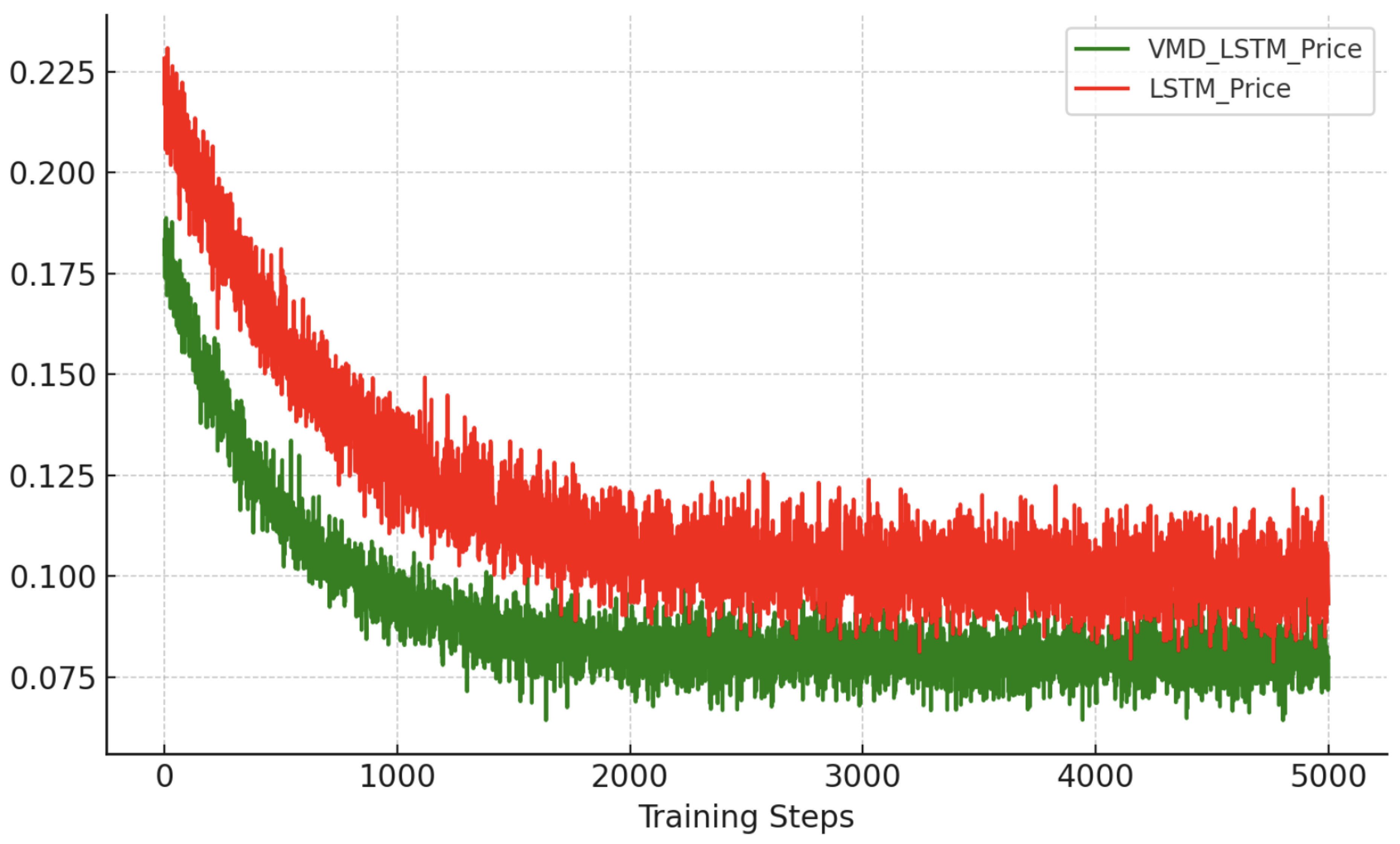
Figure 5.
Comparison of Training Loss for Return Prediction Models on CSI 300 Index
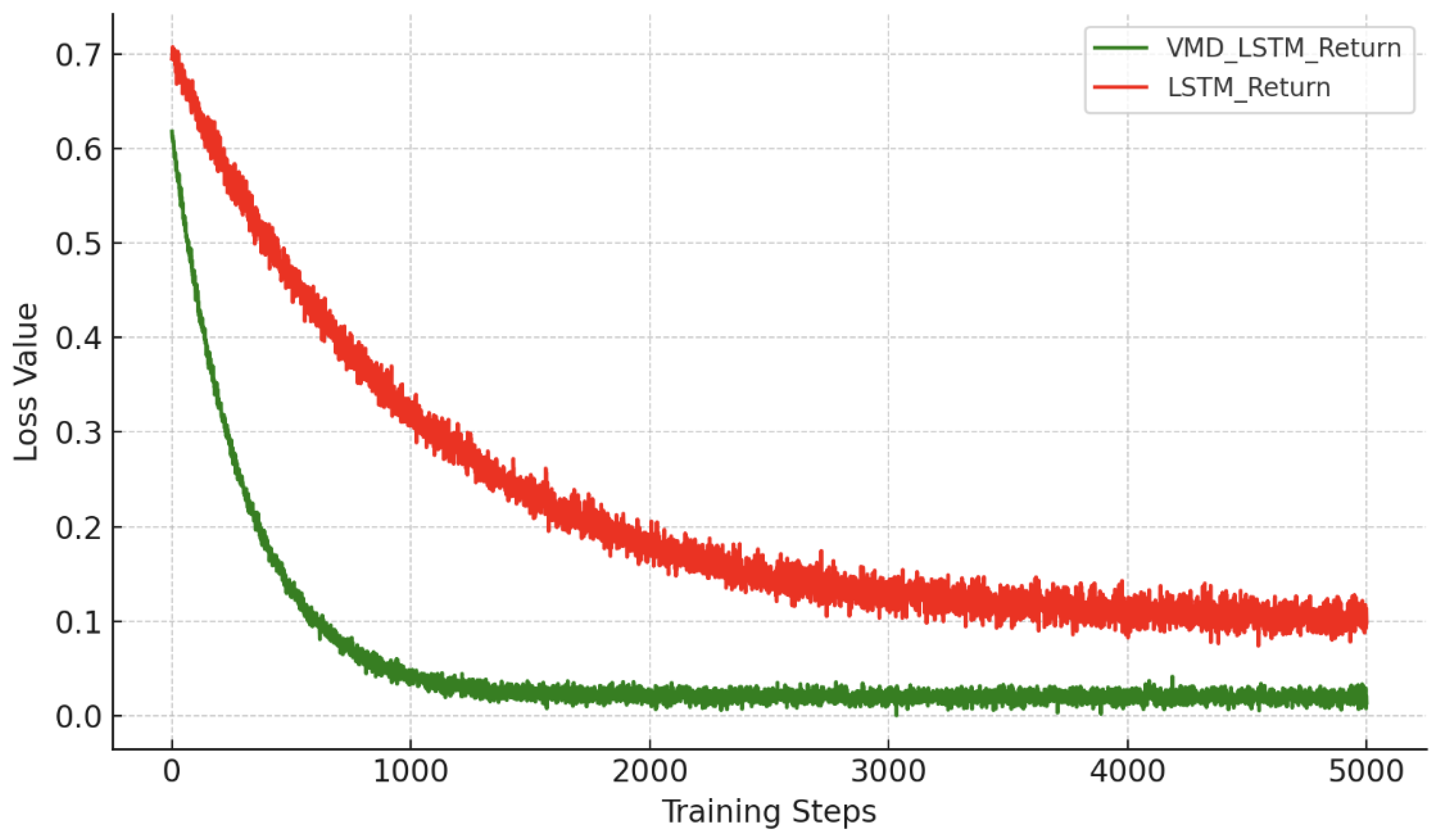
Figure 6.
Validation Accuracy Comparison of Price Prediction Models on SSE Index
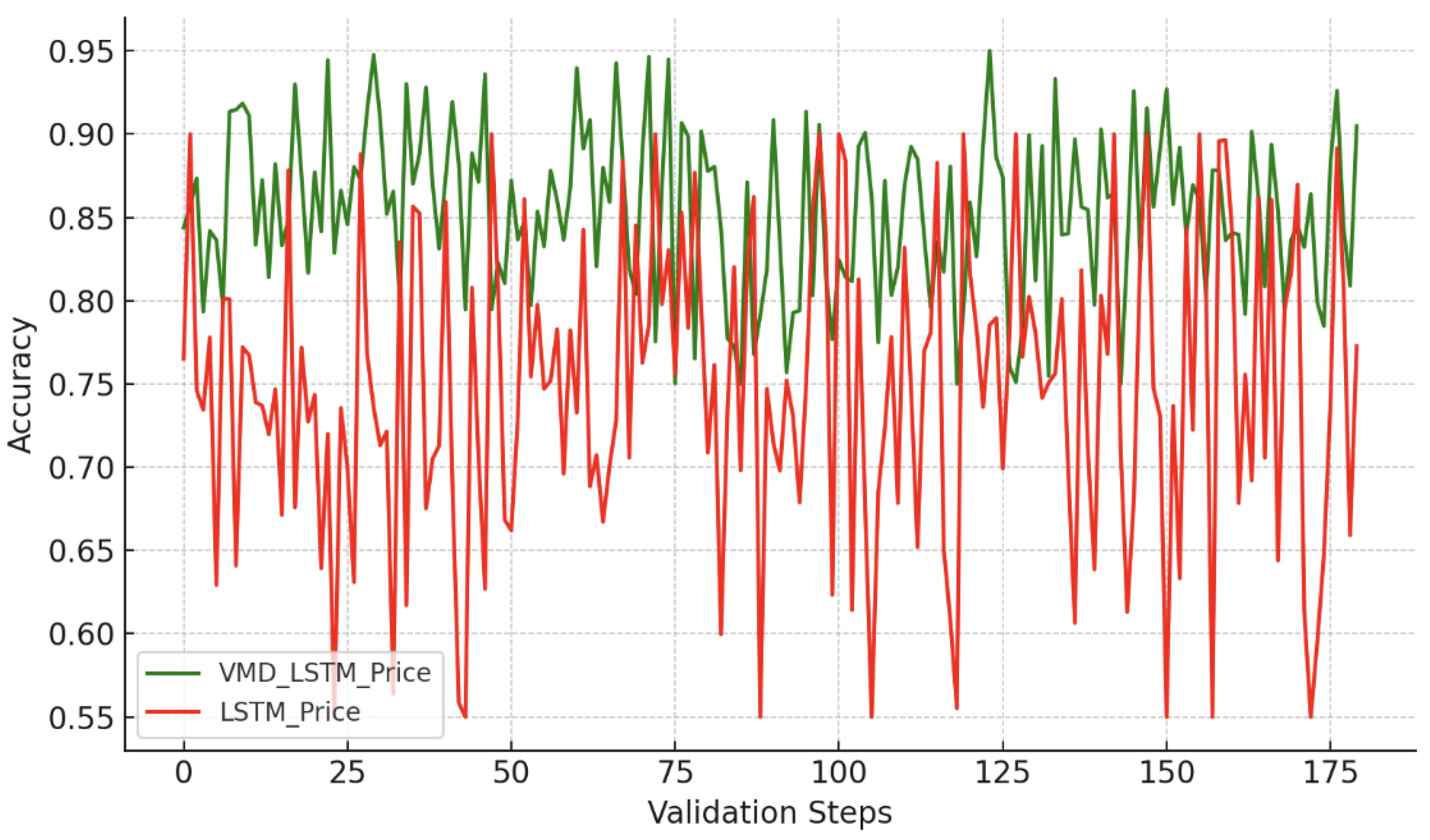
Figure 7.
Prediction Accuracy on the Validation Set for the Return Forecasting Model
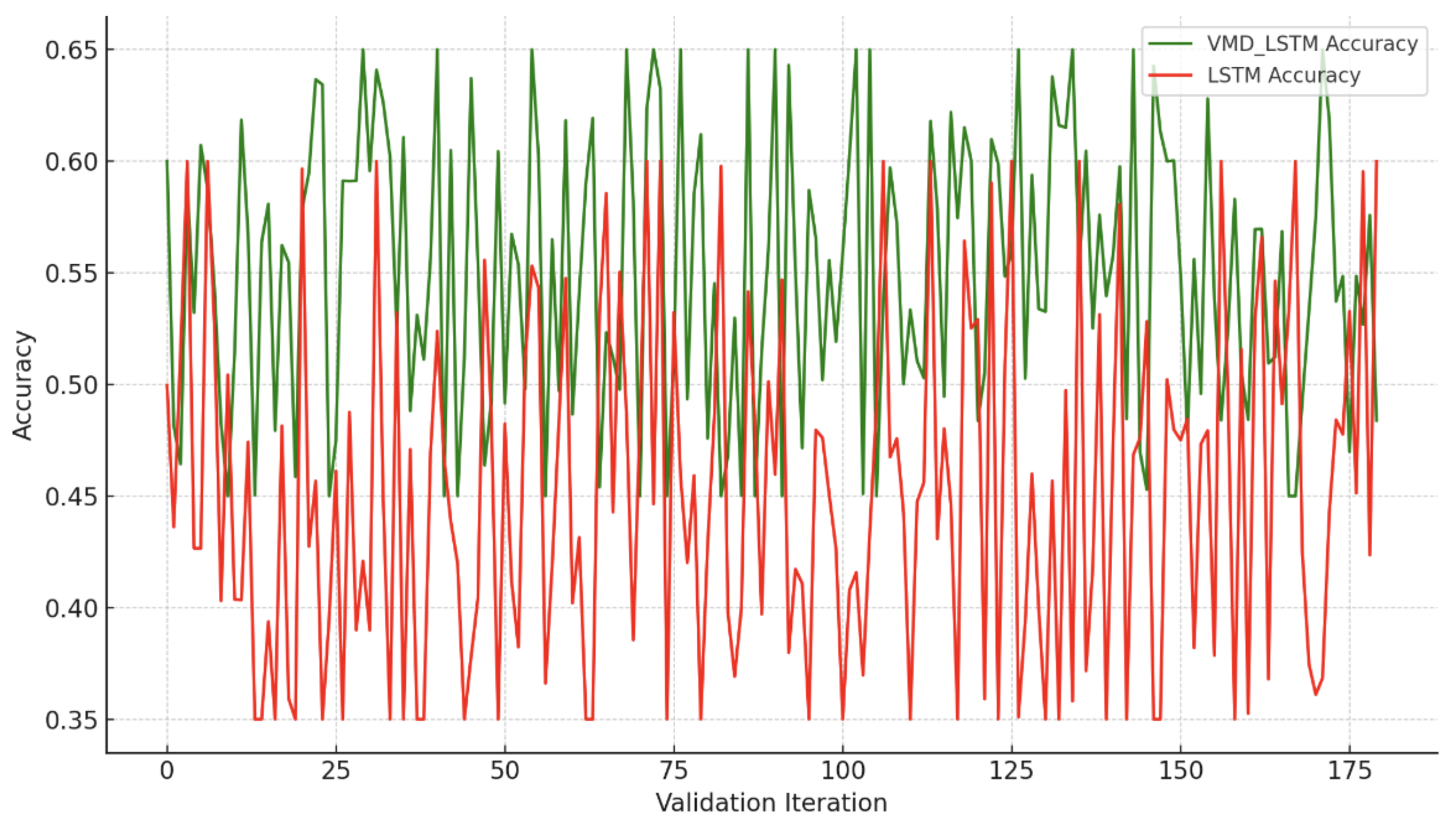

Table 1.
ADF Stationarity Test of the Two Stock Indices
| Series | ADF Statistic | p-value | 1% Level | 5% Level | 10% Level |
|---|---|---|---|---|---|
| SSE Closing Price | -2.2490 | 0.1889 | -3.437 | -2.864 | -2.568 |
| SSE Return | -15.423 | 3.0166 | -3.436 | -2.864 | -2.568 |
| CSI 300 Closing Price | -2.7361 | 0.0680 | -3.436 | -2.864 | -2.568 |
| CSI 300 Return | -13.318 | 6.5249 | -3.436 | -2.864 | -2.568 |
Table 2.
Hurst Exponent Test for Long Memory Property
Disclaimer/Publisher’s Note: The statements, opinions and data contained in all publications are solely those of the individual author(s) and contributor(s) and not of MDPI and/or the editor(s). MDPI and/or the editor(s) disclaim responsibility for any injury to people or property resulting from any ideas, methods, instructions or products referred to in the content. |
© 2025 by the authors. Licensee MDPI, Basel, Switzerland. This article is an open access article distributed under the terms and conditions of the Creative Commons Attribution (CC BY) license (http://creativecommons.org/licenses/by/4.0/).
Copyright: This open access article is published under a Creative Commons CC BY 4.0 license, which permit the free download, distribution, and reuse, provided that the author and preprint are cited in any reuse.


