
Submitted:
07 September 2025
Posted:
09 September 2025
You are already at the latest version
Abstract
Crude oil prices exhibit complex dynamics---such as volatility clustering, asymmetric temporal dependencies, and nonlinear responses to geopolitical and economic shocks---that pose challenges to accurate forecasting. To address this, we propose a hybrid model, GBK-Net, which integrates three complementary components: GARCH for modeling time-varying volatility, BiLSTM for capturing bidirectional temporal dependencies, and Kolmogorov-Arnold Network (KAN) for refining nonlinear relationships. Empirical validation is conducted on 39 years of daily WTI crude oil prices (1986--2025), covering major events such as the 2008 financial crisis and the COVID--19 pandemic. Comparative experiments against benchmark models---including GARCH, EGARCH, LSTM, and CNN--LSTM--KAN---demonstrate that GBK-Net achieves the lowest prediction error (RMSE = 2.49; R2 = 0.981), with statistical tests confirming its superiority. We also benchmark nested specifications using approximately unbiased tests [1]. This work contributes a robust forecasting tool for energy economics, with implications for strategic planning, risk hedging, and financial decision-making in volatile energy markets. Unless otherwise noted, we model and evaluate on shifted log-returns to accommodate the 2020 negative-price episode; results using arithmetic returns are reported as robustness checks in the Appendix.
Keywords:
crude oil price forecasting
; hybrid model
; GARCH
; BiLSTM
; Kolmogorov-Arnold Network
; volatility clustering
; nonlinear dynamics
1. Introduction
Crude oil, as a critical strategic resource, plays a pivotal role in global energy security, economic stability, and industrial development [2]. Its price fluctuations have far-reaching impacts on macroeconomic indicators such as inflation, employment, and trade balances [3], as well as on micro-level decision-making in industries ranging from transportation to manufacturing [4]. However, crude oil prices exhibit complex dynamics, including volatility clustering1, nonlinear temporal dependencies, and sensitivity to geopolitical events, economic policies, and supply-demand shocks [5,6]. These characteristics pose significant challenges to accurate forecasting, making it a long-standing focus in energy economics and financial research. This macro–financial nexus has been documented across regimes and markets [7,8,9,10,11].”
Accurate crude oil price forecasting is essential for multiple stakeholders. For governments, it informs energy policy formulation, strategic reserves management, and inflation control [IEA, 2022]. For energy companies, it supports investment decisions, risk hedging, and production planning [12]. For financial markets, it guides the pricing of oil-related derivatives and portfolio optimization [13]. Conversely, inaccurate forecasts may lead to market distortions, excessive speculation, or suboptimal policy responses [14]. Thus, developing robust forecasting models remains a critical research priority. See also real-time evidence on forecastability [11] and stock-market transmission [9].
Crude oil prices are influenced by a complex interplay of factors, including supply-demand fundamentals such as OPEC production quotas, shale oil extraction costs, and global energy transitions [15]; financialization through speculative activities in commodity markets that amplify price volatility [16]; and geopolitical and macroeconomic shocks like conflicts in oil-producing regions, economic recessions, or policy shifts [17]. These factors result in price dynamics that violate the assumptions of traditional linear models, such as homoskedasticity2 and stationarity [18]. Volatility clustering, for instance, indicates that past price fluctuations contain information about future volatility—a feature formalized by Engle [19] through the Autoregressive Conditional Heteroskedasticity (ARCH) model. Additionally, nonlinear relationships between drivers and bidirectional temporal dependencies further complicate forecasting [20]. Moreover, asymmetric/leverage effects motivate EGARCH/GJR/TARCH extensions [21,22,23].”
To address these challenges, researchers have developed three main categories of forecasting models, each with distinct strengths and limitations. Early efforts relied on linear time series models such as Autoregressive Integrated Moving Average [24] and its variants. While ARIMA captures linear temporal trends, it fails to model volatility clustering or nonlinearities [25]. To address volatility, [26] extended ARCH to Generalized ARCH (GARCH), which models conditional variance as a function of past squared residuals and volatility. GARCH and its variants remain widely used for volatility forecasting [27], but struggle with complex nonlinear relationships and long-range temporal dependencies [28].
With advances in computational power, machine learning models such as Support Vector Regression [29] and Random Forest [30] have been applied to capture nonlinear patterns. Deep learning (DL) models, particularly Recurrent Neural Networks (RNNs) and their variants, excel at modeling temporal sequences. Long Short-Term Memory (LSTM) networks [31] address the vanishing gradient problem in RNNs, enabling long-term dependency learning, and are widely adopted for time series forecasting [32]. Bidirectional LSTM (BiLSTM) [33] further enhances performance by processing sequences in both directions, capturing bidirectional temporal relationships [34]. However, standalone DL models often overlook volatility clustering, as they treat input data as homoscedastic [35].
Recognizing the limitations of single-model approaches, hybrid models have emerged that combine statistical and ML/DL techniques. For example, GARCH-LSTM models integrate GARCH-derived volatility with LSTM to capture both volatility and temporal dependencies [20]. Similarly, CNN-LSTM models apply convolutional layers to extract local features before feeding them into LSTM [36]. While these hybrids outperform standalone models, gaps remain: (1) few incorporate bidirectional temporal learning to capture asymmetric dependencies; (2) nonlinear refinement remains limited, as traditional activation functions may not fully model complex high-dimensional nonlinearities [37].
Notably, existing hybrid frameworks suffer from three critical gaps: (i) volatility modeling (e.g., GARCH) is often loosely coupled with sequential learning, failing to encode time-varying risk into temporal features; (ii) unidirectional LSTMs in models like GARCH-LSTM cannot capture forward-backward feedback loops—for example, how future geopolitical expectations influence current prices; (iii) nonlinear refinement relies on traditional activation functions, which underperform in approximating discontinuous jumps, such as the 2020 negative WTI prices caused by storage constraints.
Our GARCH–BiLSTM–KAN addresses these limitations by: (i) fusing GARCH-derived volatility as structured input to BiLSTM; (ii) leveraging bidirectional sequences to model expectation-driven feedback; and (iii) employing KAN’s spline-based nonlinearity to capture extreme market anomalies.
To this end, we propose a novel hybrid model—GARCH–BiLSTM–KAN—that integrates three components with complementary strengths: GARCH(1,1), which models time-varying volatility to enrich input features; BiLSTM, which captures bidirectional temporal dependencies in both returns and volatility; and the Kolmogorov–Arnold Network (KAN), a recently proposed neural architecture [37] that uses univariate basis functions to model complex nonlinearities and refine BiLSTM outputs more efficiently than traditional networks.
Using daily WTI crude oil prices from 1986 to 2025, we compare GARCH–BiLSTM–KAN with benchmark models (e.g., GARCH, LSTM, GARCH-LSTM, CNN–LSTM–KAN). The contributions of this study are threefold: (1) Methodologically, we introduce a synergistic framework that unifies volatility modeling, bidirectional sequence learning, and advanced nonlinear refinement; (2) Empirically, we demonstrate superior forecasting performance via RMSE, MAE, and , validated by statistical tests over a 39-year dataset; (3) Practically, we provide a robust tool for energy market stakeholders to support risk management, policy formulation, and investment decision-making.
The remainder of the paper is organized as follows: Section 2 details the methodology of the GARCH–BiLSTM–KAN model, including the mathematical formulations of each component and their integration. Section 3 describes the data, including sources, preprocessing, and descriptive statistics. Section 4 presents empirical results, comparing the proposed model with benchmark models. Section 5 discusses the implications of the findings, while Section 6 concludes with limitations and directions for future research. Throughout, the forecasting target is the one-step-ahead shifted log-return (Section 3); price-level forecasts are reconstructed for comparability across model families (Section 4).
2. Methodology
This section presents the methodological framework of the proposed GARCH–BiLSTM–KAN hybrid model (hereafter referred to as GBK-Net), which integrates three complementary components: GARCH for modeling time-varying volatility, BiLSTM for capturing bidirectional temporal dependencies, and KAN for refining complex nonlinear relationships. The architecture is designed to address the inherent challenges of financial time series, such as volatility clustering, temporal asymmetry, and nonlinear dynamics. Figure 1 provides a schematic overview of the GBK-Net framework.
2.1. GARCH for Volatility Estimation
The Generalized Autoregressive Conditional Heteroskedasticity (GARCH) model, originally proposed by Bollerslev [26], constitutes the foundational component for volatility estimation in the GBK-Net framework. Financial time series, particularly asset returns, often exhibit volatility clustering—a stylized fact where periods of high volatility are likely to be followed by high volatility, and low volatility by low volatility. This behavior violates the homoskedasticity assumption inherent in classical linear models. GARCH addresses this by modeling the conditional variance as a function of both past squared residuals and past conditional variances, allowing it to effectively capture time-varying volatility dynamics.
For a given time series of returns , the GARCH specification consists of two equations: the mean equation and the variance equation. The mean equation is defined as:
where is the constant mean return, and is the error term at time t, which follows a conditional normal distribution with representing the information set up to time .
The conditional variance , which measures the volatility, is specified in the GARCH variance equation as:
where is the constant term, are the ARCH coefficients capturing the impact of past squared residuals (news about volatility from the recent past), and are the GARCH coefficients representing the persistence of volatility. To ensure the positivity and stationarity of the conditional variance, the parameters must satisfy:
In our hybrid model, we employ the GARCH (1,1) variant, which is parsimonious and widely documented to effectively capture volatility dynamics in financial data [26,27]. The estimated conditional volatility from GARCH (1,1) serves as a critical input to the subsequent BiLSTM and KAN components, providing a structured measure of historical volatility that complements the raw return series. For completeness, asymmetric volatility alternatives include EGARCH, GJR-GARCH and TARCH [21,22,23].”
2.2. BiLSTM for Bidirectional Temporal Learning
While GARCH models excel at volatility estimation, they are limited in capturing complex temporal dependencies, especially those involving long-range interactions and bidirectional relationships. To address this, we integrate a Bidirectional Long Short-Term Memory (BiLSTM) network, an extension of the LSTM architecture [31], which is designed to model sequential data by preserving information from both past and future time steps.
LSTM networks overcome the vanishing gradient problem of traditional Recurrent Neural Networks (RNNs) through a gated cell structure, enabling them to learn long-term dependencies. Each LSTM cell contains three key gates: the forget gate, input gate, and output gate, which regulate the flow of information into and out of the cell state .
Forget Gate: Determines which information to discard from the cell state:
Input Gate: Controls the update of the cell state with new information:
Cell State Update: Combines the forget gate output and input gate output:
Output Gate: Determines the hidden state based on the cell state:
where is the sigmoid activation function, ∘ denotes element-wise multiplication, is the input at time t, is the hidden state from the previous time step, and W and b are weight matrices and bias vectors, respectively.
The BiLSTM (Bidirectional Long Short-Term Memory) architecture consists of two parallel LSTM networks: a forward LSTM that processes the sequence from past to future ( to ) and a backward LSTM that processes it from future to past ( to ). The hidden states from both directions are concatenated at each time step to form the final output, capturing both historical and future contextual information:
In our model, the input to the BiLSTM layer includes both the raw return series and the GARCH-estimated volatility , forming a multivariate input sequence:
A Lookback Window of 20 is used to construct input sequences, meaning each sample contains 20 time steps of historical data. At inference, inputs are sliding windows . The BiLSTM encodes the within-window sequence bidirectionally; no information beyond time t is used. The BiLSTM is configured with 32 hidden units in each direction (64 after concatenation) and 2 layers, trained using the Adam optimizer with a learning rate of 0.01 [38]. This allows the BiLSTM to learn temporal patterns in both returns and volatility, with the bidirectional design enabling it to capture asymmetric dependencies. The output of the BiLSTM, , is a high-dimensional representation of bidirectional temporal features, which is fed into the KAN layer for further refinement. Figure 2 shows the schematic diagram of hidden state fusion process in BiLSTM.
2.3. KAN for Nonlinear Refinement
Despite the strength of BiLSTM in modeling temporal dynamics, financial time series often exhibit highly nonlinear relationships that are challenging to capture with standard neural network architectures. To address this, we incorporate a Kolmogorov-Arnold Network (KAN) (Liu et al., 2024) [37], a novel neural network paradigm that leverages the Kolmogorov-Arnold representation theorem [39] to model complex nonlinear functions through a combination of univariate functions and linear operations.
Kolmogorov–Arnold Networks (KANs) differ from traditional feedforward neural networks in their internal transformation mechanism. In conventional neural networks, each layer typically applies a linear transformation followed by a nonlinear activation function. In contrast, KANs replace this with a structure based on univariate basis functions and linear combination.
Specifically, for a KAN with input dimension d and output dimension m, the transformation of an input vector is defined as:
where denotes the univariate basis function applied to the i-th input for the k-th output, are trainable weights, and are bias terms.
In this work, the KAN layer uses cubic B-spline basis functions with 5 knots per input dimension. Knot locations are initialized at empirical quantiles of each input feature and are fine-tuned jointly with the spline coefficients and output weights via backpropagation. We adopt Xavier initialization for weights and apply regularization to the spline coefficients; early stopping is used to prevent overfitting. This piecewise-polynomial parameterization provides local, stable nonlinear refinement of the BiLSTM features without invoking radial basis functions or Gaussian centers/widths. As a result, they reduce the number of learnable parameters compared to fully connected networks while preserving strong expressive power.
In our framework, the KAN receives the output of the BiLSTM layer, , as input. The KAN has a width structure of and uses cubic B-spline basis functions with 5 knots for . These functions are selected due to their flexibility in approximating smooth nonlinearities and their high interpretability [37].
The KAN is optimized using the Adam optimizer with a learning rate of 0.01. Its role is to enhance the modeling of residual nonlinear dependencies that are not fully captured by the GARCH and BiLSTM components. The output of the KAN, denoted , represents the refined prediction after accounting for both temporal dependencies and nonlinear patterns. Figure 3 shows the schematic diagram of the KAN model structure.
Our lightweight KAN head (width ) and mild regularization are also motivated by graph-theoretic sparsity notions. The maximum forcing number characterizes the smallest edge set ensuring structural uniqueness, while conditional matching-preclusion quantifies the least deletions that destroy perfect matchings [40,41]. By analogy, we seek the smallest set of active channels that preserves identifiability of nonlinear mappings—achieving parameter economy without sacrificing predictive fidelity.
2.4. Hybrid Model Integration of GARCH–BiLSTM–KAN
The GBK-Net hybrid model is integrated in a sequential manner, where each component’s output serves as input to the next, leading to the final prediction. For the implementation of this model, we adopt a one-step-ahead walk-forward prediction strategy: at each time point t, the GBK-Net model is trained using data from the time interval to predict the data at time ; all data standardization tools (scalers) are only fitted based on the training set data (i.e., the data from used for model training at time t), and the prediction results are inverted back to the original data scale before calculating the prediction error; unless otherwise specified, the prediction period is 1 day. Table 1 summarizes the key parameters of each component in the GBK-Net hybrid model.
1. GARCH Preprocessing: The raw return series is first fed into the GARCH(1,1) model to estimate the conditional variance (volatility). This step transforms the univariate return series into a two-dimensional feature vector , enriching the input with volatility information.
2. BiLSTM Feature Extraction: The two-dimensional feature sequence is fed into the BiLSTM network, which processes it bidirectionally (forward and backward) to generate bidirectional temporal features . The network uses a Lookback Window of 20 to construct input sequences, with 32 hidden units per direction and 2 layers, trained using the Adam optimizer with a learning rate of 0.01.
3. KAN Refinement: The GBK-Net features are input to the KAN, which applies cubic B-spline basis functions (with 5 knots) to each feature dimension, followed by a linear combination to yield the final prediction . The KAN has a width structure of and uses the same Adam optimizer.
The sequential integration is theoretically motivated by the “hierarchical feature refinement” principle: GARCH first decomposes raw returns into predictable volatility patterns, reducing noise for subsequent layers. BiLSTM then encodes bidirectional dependencies—forward LSTMs capture supply-driven trends, while backward LSTMs model demand expectations. Finally, KAN refines these temporal features using cubic B-splines, which outperform ReLU in approximating non-smooth functions. Consequently, this pipeline ensures that volatility, temporal asymmetry, and nonlinearity are modeled as interdependent rather than isolated phenomena.
4. Training and Loss Function: The entire model is trained end-to-end for 100 epochs using the mean squared error (MSE) loss function, defined as:
where is the true value and is the model’s prediction. Three evaluation metrics are used to assess performance:
Root Mean Squared Error (RMSE):
Mean Absolute Error (MAE):
Coefficient of Determination ():
The model is trained on 80% of the data (7,877 samples) and tested on the remaining 20% (1,969 samples) using a time-series split to avoid data leakage from future to past. The price data are normalized using the MinMaxScaler with a feature range of , which improves training stability and convergence for the BiLSTM architecture.
The integration of GARCH, BiLSTM, and KAN is motivated by their complementary strengths: GARCH provides a statistically grounded measure of volatility, BiLSTM captures bidirectional temporal dependencies in both returns and volatility, and KAN refines these features by modeling residual nonlinearities. This hierarchical approach ensures that the model leverages both parametric (GARCH) and nonparametric (BiLSTM, KAN) techniques, making it robust to the diverse characteristics of financial time series, which single-model approaches often fail to address.
The hyperparameter settings are summarized in Table 1.
From a robustness perspective, our design is informed by connectivity and restricted-connectivity results in high-dimensional interconnection networks. Studies on k-ary n-cubes, m-ary hypercubes, and locally twisted cubes analyze minimal cut sets and extra/restricted edge-connectivity, offering a structural analogy for how performance degrades when feature channels or links are perturbed [42,43,44,45,46]. Related results on leaf-sort graphs connect connectivity with matching preclusion, motivating our choice to keep a small but reliable set of pathways in the hybrid pipeline rather than many fragile ones [47,48].
3. Data Description
This study uses daily price data of West Texas Intermediate (WTI) crude oil, a widely recognized benchmark for global oil markets (U.S. Energy Information Administration [EIA], 2023). WTI is favored for its high liquidity and frequent use in pricing agreements. The dataset covers 9,866 daily observations over 39 years, from January 2, 1986, to March 10, 2025. This period encompasses diverse market conditions, including economic expansions, recessions, geopolitical crises, and energy policy changes. Such variety is essential for evaluating the robustness of the proposed forecasting model. Historical evidence further underscores regime shifts and asymmetric macro effects [7,8].”
The raw WTI crude oil price data were obtained from the U.S. Energy Information Administration (EIA) database3, a widely trusted source for energy market data (EIA, 2023). Additional validation was conducted using historical records from the Federal Reserve Economic Data (FRED) database4, maintained by the Federal Reserve Bank of St. Louis, to ensure consistency.
To handle both non-stationarity and the 2020 negative prices, we first shift prices by a positive constant C so that logarithms are well defined:
Daily shifted log-returns are then computed as
Unless otherwise specified, serves as the default target for model training and evaluation. All price-like inputs are normalized by a MinMaxScaler to after the shift in (19); metrics are reported on the original (unshifted) price scale after inverting the transformation during evaluation.
Additionally, all price data were normalized using Min–Max Normalization (MinMaxScaler) with a feature range of to standardize input values. This standardization enhances the convergence speed of neural network components (BiLSTM and KAN) during training [49].
Table 2 summarizes the key descriptive statistics of the WTI crude oil prices over the sample period. The mean price is , with a standard deviation of , indicating significant price volatility—a characteristic consistent with previous studies on energy commodities [50]. The median price is , slightly lower than the mean, suggesting a right-skewed distribution, which is typical of commodity prices influenced by supply shocks. The interquartile range (IQR) is calculated as:
which further highlights the substantial price variability over the period. Over the sample period, prices range from a minimum of , observed during the 2020 COVID–19 crisis when storage constraints led to negative prices [51], to a maximum of during the 2008 global financial crisis, driven by supply concerns [3].
Figure 4 presents the trend of WTI crude oil prices from 1986 to 2025, highlighting several notable periods. From 1986–1992, prices remained relatively stable, averaging around USD 20.00–30.00 per barrel, reflecting balanced supply–demand dynamics [52]. Between 2000–2008, prices exhibited a sharp upward trend, peaking at USD 145.31 in 2008 due to rapid economic growth in emerging markets and geopolitical tensions in the Middle East [53]. The 2014–2016 crash saw prices fall from over USD 100.00 to below USD 30.00, driven by a supply glut from U.S. shale oil production and OPEC’s decision to maintain output [54]. In April 2020, during the COVID–19 pandemic, prices reached an unprecedented USD -36.98 as lockdowns triggered a collapse in demand [55]. The post-2020 recovery was marked by a gradual rebound, influenced by economic reopening, supply chain disruptions, and geopolitical conflicts. Figure 5 illustrates the first difference of WTI prices, representing daily price changes, and confirms the presence of volatility clustering—periods of high volatility (e.g., 2008, 2020) interspersed with relatively calm intervals—supporting the inclusion of volatility-modeling components such as GARCH in the GBK-Net hybrid framework [26].
To evaluate the out-of-sample forecasting performance of GBK-Net, the dataset was split into a training set (80%, 7,877 observations, 1986–2016) and a testing set (20%, 1,969 observations, 2017–2025). This chronological split ensures that the model is trained exclusively on historical data and tested on more recent observations, enabling it to capture evolving market dynamics. The testing period includes major events such as the COVID–19 pandemic and the Russia–Ukraine conflict, providing a realistic assessment of the model’s robustness under changing macroeconomic and geopolitical conditions [25].
4. Empirical Results
To systematically evaluate the predictive efficacy of the proposed GBK-Net, a comprehensive comparative analysis was conducted against multiple benchmark models, including traditional volatility models (GARCH, EGARCH), standalone deep learning architectures (LSTM), and hybrid configurations (LSTM-KAN, GARCH-LSTM, CNN-LSTM, CNN–LSTM–KAN).
Given the differences between the output forms of statistical models (GARCH/EGARCH, which predict a conditional mean of returns) and deep learning models (which output prices directly), we reconstruct all statistical-model forecasts to the same price target before scoring. We proceed in two steps.
so that and log-returns are well defined even in the presence of negative prices.
If a model outputs the one-step-ahead shifted log-return , we reconstruct price via
If a model outputs the arithmetic return , we use
In all cases, evaluation metrics (RMSE, MAE, ) are computed on the original (unshifted) price scale by comparing with . By default we fit and report shifted log-returns; arithmetic-return variants are included only where explicitly noted and are mapped back using (24).
Three performance metrics—root mean squared error (RMSE), mean absolute error (MAE), and coefficient of determination ()—were computed on the out-of-sample test set. The results are summarized in Table 3 for direct comparison across models.
As shown in Table 3, GBK-Net achieved the best performance across all evaluation metrics, registering the lowest RMSE (2.4876) and MAE (1.5156), along with the highest value (0.9810). This indicates that the model explains approximately 98.10% of the variance in observed WTI crude oil prices, reflecting a strong fit to the underlying process. Among the hybrid alternatives, CNN–LSTM–KAN ranked second, with slightly higher errors (RMSE = 2.6047, MAE = 1.6464) and a marginally lower (0.9792). The CNN-LSTM architecture, while effective at capturing local spatiotemporal patterns, produced comparatively inferior results (RMSE = 2.7639, MAE = 1.7693, = 0.9765), underscoring the incremental value of integrating KAN for nonlinear feature refinement.
Figure 6.
Local Comparison of Prediction Results of Various Models on the Test Set
Beyond the top-performing GBK-Net, we examined standalone deep learning architectures and simpler hybrids. Standalone deep learning models exhibited comparatively diminished performance: the LSTM network achieved an RMSE of 2.8802, MAE of 1.8445, and of 0.9745, while the LSTM-KAN hybrid showed a marginal decline in predictive accuracy (RMSE = 2.9223, MAE = 1.8780, = 0.9738). This suggests that KAN’s nonlinear mapping relies on the prior integration of volatility modeling and bidirectional temporal learning components to achieve optimal performance. The GARCH-LSTM model, which combines volatility estimation with unidirectional sequence processing, demonstrated a higher error profile (RMSE = 3.0753, MAE = 1.9996) and lower (0.9710) compared with the proposed framework, highlighting the importance of bidirectional temporal dependency modeling for capturing asymmetric price dynamics.
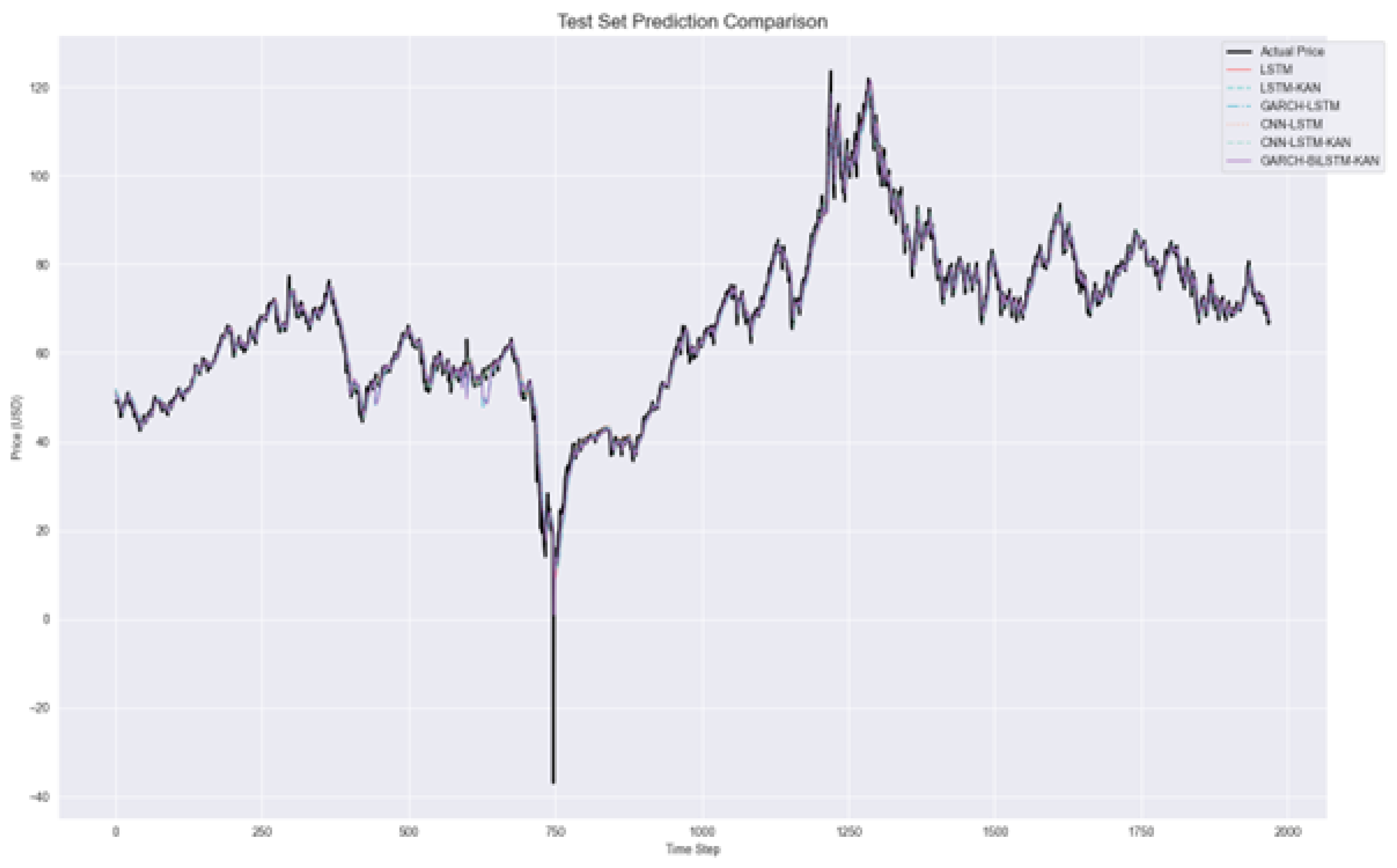
Figure 7.
Comparison of test set predictions among effective models (LSTM, LSTM-KAN, GARCH-LSTM, CNN-LSTM, CNN–LSTM–KAN, and GBK-Net) against the actual WTI crude oil prices. The curves closely overlap, highlighting the superior alignment of GBK-Net with observed prices.
Figure 7.
Comparison of test set predictions among effective models (LSTM, LSTM-KAN, GARCH-LSTM, CNN-LSTM, CNN–LSTM–KAN, and GBK-Net) against the actual WTI crude oil prices. The curves closely overlap, highlighting the superior alignment of GBK-Net with observed prices.
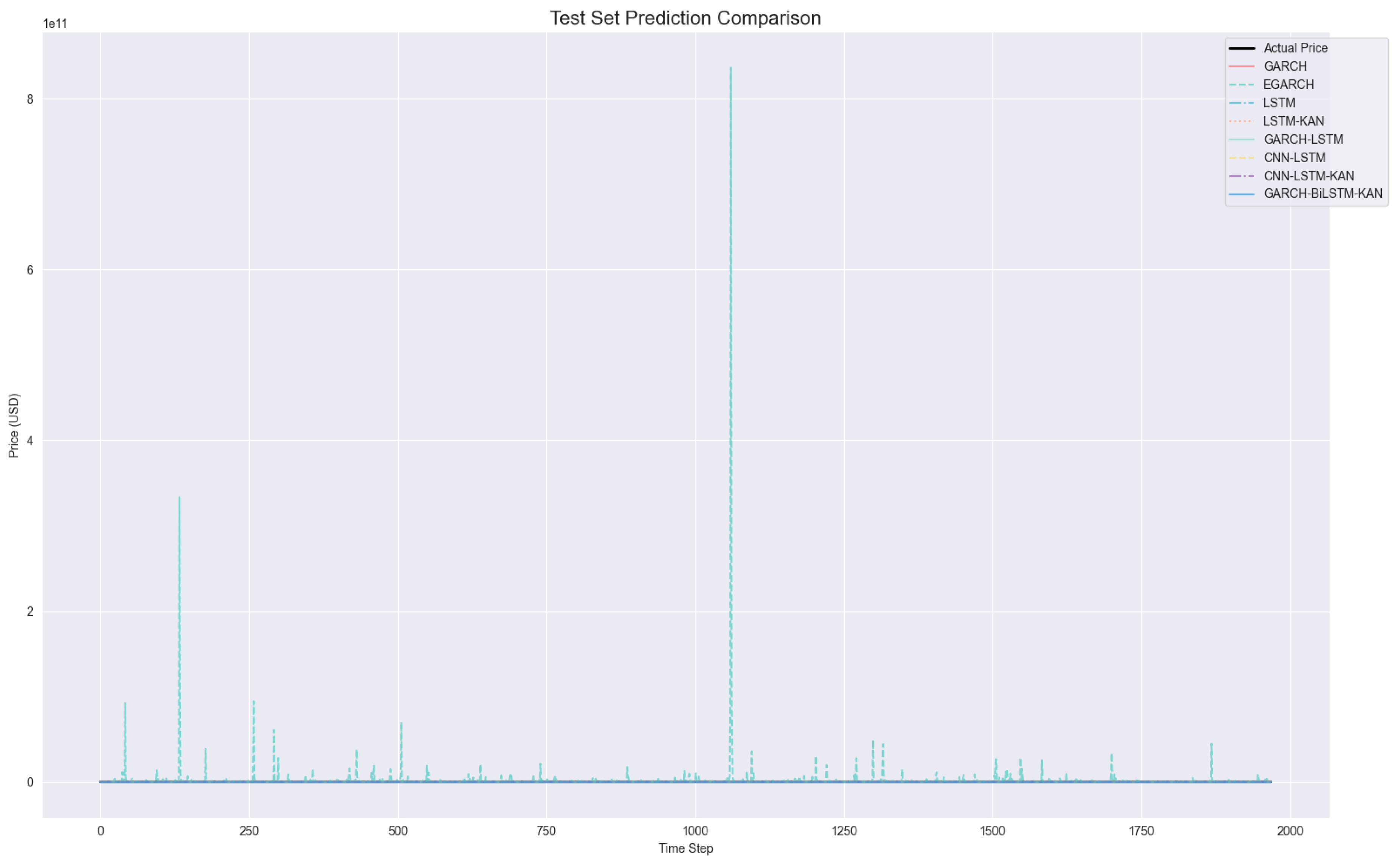
Figure 8.
Comparison of test set predictions including all models (GARCH, EGARCH, LSTM, LSTM-KAN, GARCH-LSTM, CNN-LSTM, CNN–LSTM–KAN, and GBK-Net). The extreme deviations of GARCH and EGARCH dominate the scale, illustrating their numerical instability and poor suitability for crude oil price forecasting.
Due to these excessively large deviations and much lower values, directly displaying GARCH and EGARCH results alongside other models in the same figures would obscure the finer prediction details and distort the comparative visualization of more effective models (e.g., GBK-Net, CNN–LSTM–KAN). Accordingly, We provide two complementary views: Figure 8 includes all models (revealing scale dominance by GARCH/EGARCH), whereas Figure 7 and the dual-panel Figure 10 focus on effective models to expose fine-grained differences.
Visual corroboration of these quantitative results is provided in Figure 6, Figure 7, Figure 8, Figure 9 and Figure 10. Figure 6 presents a localized comparison of test set predictions, where GBK-Net forecasts exhibit close alignment with actual prices, in contrast to the substantial deviations observed in GARCH and EGARCH. This superior alignment is further evidenced in Figure 7 and Figure 8, which zooms into a sub-period of the test set, revealing the model’s ability to capture both short-term fluctuations and medium-term trends more effectively than CNN–LSTM–KAN and other LSTM-based architectures, which display noticeable lag effects and overshooting.
Training dynamics in Figure 9 compare MSE loss over 100 epochs. All models descend steeply within the first 10–20 epochs and then flatten, indicating fast optimization. GBK-Net (GARCH–BiLSTM–KAN) and CNN–LSTM–KAN converge earlier with smaller oscillations, reflecting the stabilizing effect of combining volatility modeling with nonlinear refinement. Plain LSTM and CNN–LSTM show larger early-epoch jitter, and GARCH–LSTM reduces loss steadily but reaches its plateau later. By 50 epochs, training losses are already near zero for most models, so performance differences are better judged on the test set (Table 3), where GBK-Net remains the top performer. Overall, the sequential integration of GARCH, BiLSTM, and KAN improves both convergence speed and training stability.
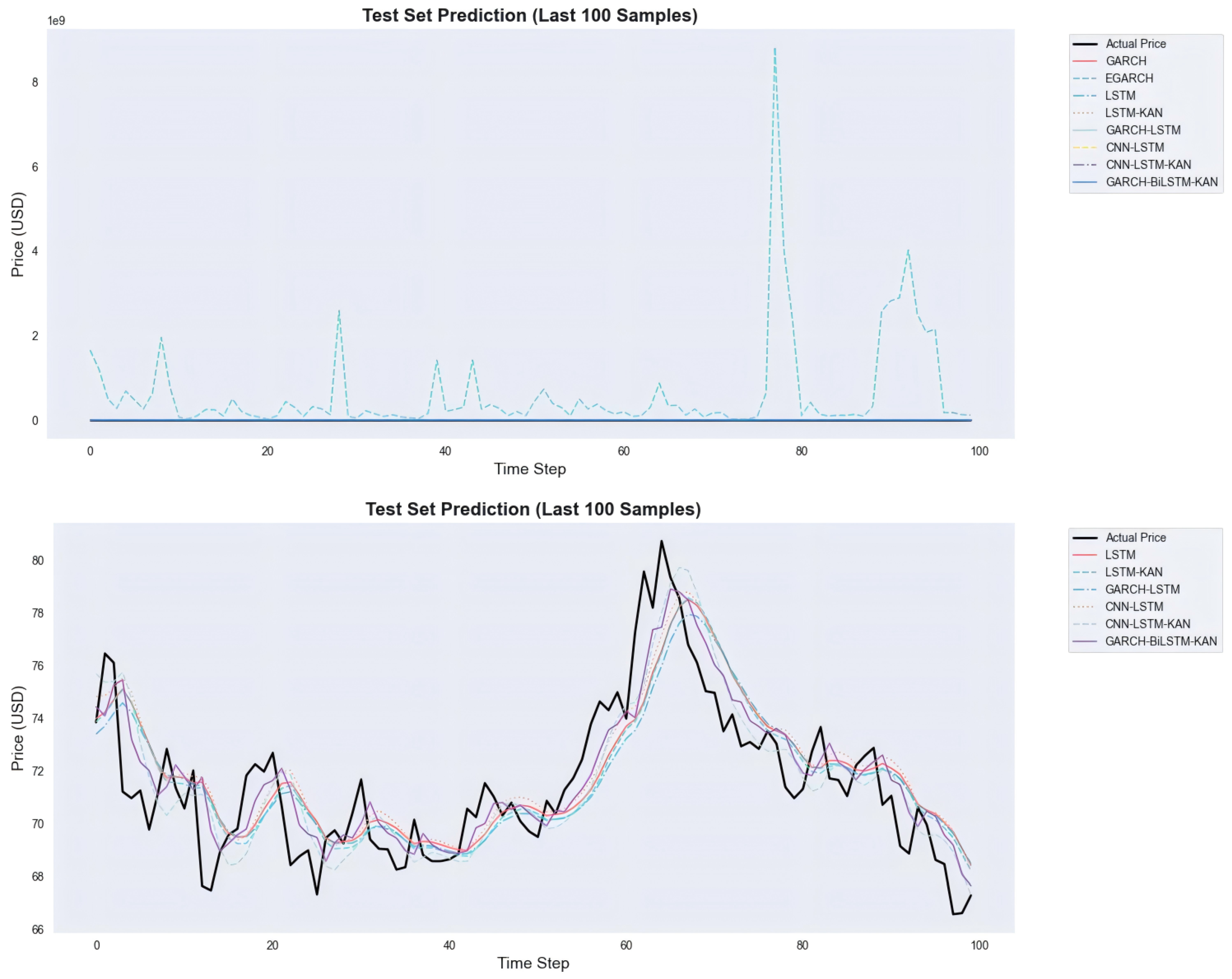
Figure 10 presents a zoomed-in view of the last 100 test samples in two panels, with the dual-panel design explicitly intended to resolve visual ambiguity caused by traditional volatility models: the top panel includes all models (GARCH, EGARCH, LSTM, LSTM-KAN, GARCH-LSTM, CNN-LSTM, CNN–LSTM–KAN, GBK-Net), where the y-axis scale is dominated by the extreme prediction spikes of GARCH/EGARCH—these spikes stem from numerical divergence and mismatched prediction targets, compressing the curves of other models into nearly indistinguishable lines, and this panel is designed to directly demonstrate the severe inadequacy of GARCH/EGARCH for crude oil price forecasting; the bottom panel excludes GARCH/EGARCH to focus solely on effective models, aiming to eliminate scale distortion and clearly reveal performance differences among competitive models: GBK-Net aligns closest with the actual price series, especially capturing the sharp upswing and subsequent correction (time steps 60–80) with smaller phase lag and less amplitude damping, while CNN–LSTM–KAN underestimates abrupt changes, plain LSTM/CNN-LSTM show noticeable lag, and GARCH-LSTM responds slowly near peaks.
Figure 10.
Last 100 test samples. Top—all models incl. GARCH/EGARCH; Bottom—effective models only.
In order to verify the contribution of GARCH volatility features, BiLSTM time-series modelling module, and KAN nonlinear fitting module to the forecasting performance of WTI crude oil price, this study designs three sets of core ablation experiments, using the original model "GARCH–BiLSTM–KAN" as a benchmark, and removing or replacing the target modules one by one by the "control single variable" principle to compare the forecasting accuracy (RMSE, MAE, ) and training efficiency of each model on the test set. The original model "GARCH–BiLSTM–KAN" is used as the baseline, and the target modules are removed or replaced one by one by the principle of "controlling a single variable", and the prediction accuracies (RMSE, MAE, and ) and training efficiencies of the models are compared with each other on the test set.
From the Table 4, GBK - Net has the best performance in terms of metrics, indicating that its architecture integrating GARCH volatility, BiLSTM time-series modelling and KAN nonlinear fitting is able to effectively capture the complex characteristics of crude oil prices; the GARCH - KAN model with the ablation of BiLSTM, due to the loss of the time-series dependence capturing ability, the RMSE and MAE increase significantly, and The GARCH - BiLSTM - FC model with KAN ablation has limited nonlinear fitting ability and inferior indexes than GBK - Net, which demonstrates the advantage of KAN in adapting to complex nonlinear relationships; the BiLSTM - KAN model with GARCH ablation has less prediction accuracy than GBK - Net due to missing volatility information, which demonstrates that the GARCH volatility model has less prediction accuracy than GBK - Net, which proves that the GARCH volatility model has less prediction accuracy than GBK - Net. Net, which proves that GARCH volatility can help identify the risk of price fluctuations. In conclusion, crude oil price prediction requires the integration of multi-module capabilities, and the fusion architecture of GBK-Net is more suitable for its characteristics.
Collectively, these empirical findings provide compelling evidence for the superiority of GBK-Net in crude oil price forecasting, demonstrating consistent superiority across both quantitative metrics and qualitative visual analyses. This validates the effectiveness of synergistically integrating volatility modeling, bidirectional temporal learning, and advanced nonlinear refinement to address the multifaceted characteristics of crude oil price dynamics.
5. Discussion
The empirical findings in Section 4 underscore the superior performance of the GARCH–BiLSTM–KAN hybrid model (GBK-Net) in forecasting WTI crude oil prices, consistently outperforming both traditional volatility models and alternative hybrid architectures across key evaluation metrics. This section discusses the theoretical and practical implications of these results, situates them within the existing literature, and identifies potential avenues for further investigation.
The outperformance of GBK-Net stems from the synergistic integration of its three components, each targeting a distinct characteristic of crude oil price dynamics. First, the GARCH(1,1) module captures volatility clustering—a defining feature of energy markets [26]—by embedding historical volatility estimates into the input sequence, thus enriching the feature space and mitigating the homoskedasticity assumption inherent in many deep learning models [35]. Second, the BiLSTM layer builds on this volatility-informed input by modeling bidirectional temporal dependencies, enabling the capture of asymmetric relationships between past and future price movements—an advantage over unidirectional LSTM or GARCH-LSTM configurations, which struggle with complex sequential asymmetries [14]. Third, the KAN module refines these bidirectional features through cubic B-spline basis functions, efficiently modeling high-dimensional nonlinearities that standard activation functions may overlook [37]. This hierarchical refinement—from volatility estimation to bidirectional sequence learning to nonlinear feature tuning—explains the model’s ability to account for of price variance in the test set (, see Table 3).
These results contribute to the ongoing discussion on the relative merits of statistical versus machine learning (ML) approaches in time series forecasting. Statistical models such as GARCH and EGARCH performed poorly, with implausibly high error metrics and strongly negative values, confirming their inability to capture the nonlinear and multifaceted nature of crude oil price dynamic [28]. In contrast, standalone ML models (e.g., LSTM, LSTM-KAN) outperformed pure statistical methods but still fell short of GBK-Net, highlighting the necessity of explicitly modeling volatility rather than relying solely on sequential pattern extraction. Likewise, the GARCH-LSTM hybrid, while incorporating volatility estimation, underperformed GBK-Net, underscoring the added value of bidirectional temporal learning in modeling asymmetric price responses to shocks.
Consistent with recent studies advocating for hybrid frameworks that combine statistical rigor with ML flexibility [20,36], our findings extend the literature by quantitatively demonstrating the incremental benefits of bidirectional temporal learning and advanced nonlinear refinement: incorporating BiLSTM yields a improvement in over GARCH-LSTM, while integrating KAN further improves by over CNN-LSTM. These quantified gains highlight the practical significance of the proposed architecture in high-volatility commodity markets.
Practically, the GARCH–BiLSTM–KAN (GBK-Net) model offers a robust tool for stakeholders in energy markets. For policymakers, its high accuracy enhances the reliability of energy policy simulations, strategic reserve planning, and inflation forecasts. Energy companies can leverage its volatility-aware predictions to improve risk hedging strategies and production planning, particularly during periods of market turbulence (e.g., the 2020 COVID–19 crisis or the 2022 Russia–Ukraine conflict, as observed in Figure 9). Financial market participants, including traders and portfolio managers, may benefit from more precise pricing of oil derivatives and optimized asset allocation, reducing exposure to forecast errors [13]. Notably, the model’s performance remains strong across diverse market conditions—from the 2008 financial crisis to the post-2020 recovery, encompassing both bull and bear phases—suggesting generalizability to both stable and volatile periods.
Our handling of extreme events and noisy inputs parallels graph-diagnosability frameworks. In g-good-neighbor and comparison diagnosis models on Cayley/star-like networks, faults can be located under limited probes provided certain observability constraints hold [56,57]. This perspective supports our joint use of volatility cues (GARCH) and bidirectional temporal context (BiLSTM) to make anomalies identifiable rather than merely smoothed; the leaf-sort results that unify connectivity and diagnosability further justify coupling “risk (volatility) signals” with sequence features to maintain identifiability during shock periods [58].
Despite its strengths, this study has limitations that warrant consideration. First, the analysis focuses exclusively on WTI crude oil; future research should validate the model’s performance on other benchmarks or related commodities such as Brent crude or natural gas to assess its broader applicability. Second, while KAN improves nonlinear modeling, its interpretability remains limited compared to parametric models. Exploring explainable AI techniques to unpack the KAN layer’s contributions—for example, identifying which basis functions drive specific price predictions to facilitate regulatory compliance and strategic transparency—could enhance trust among practitioners. Third, the model’s input features are restricted to historical prices and volatility. Incorporating external variables such as macroeconomic indicators, geopolitical risk indices, or OPEC production data may further improve predictive power, as these factors are known to influence oil prices [15,25], with Kilian [15] emphasizing macroeconomic factors and Hyndman & Athanasopoulos [25] focusing on forecasting methodologies.
Looking forward, attention-based fusion across heterogeneous exogenous signals may further enhance GBK-Net. Self-attention offers a principled way to model cross-type dependencies in heterogeneous networks (e.g., the Temporal Fusion Transformer for interpretable multi-horizon time-series forecasting [59]), while multimodal pipelines in high-throughput sensing align and fuse image/sensor/text channels to improve robustness under distributional shift [60,61,62]. In our setting, an attention-driven fusion block could integrate macroeconomic series, inventories, shipping indices, option-implied measures, and news sentiment, enabling context-conditioned regime detection that complements volatility cues from GARCH and temporal features from BiLSTM.
On the efficiency side, recent work in applied vision for agriculture demonstrates that lightweight deep networks can retain accuracy while sharply reducing parameters and energy cost—enabling field deployment and real-time inference [63,64]. Inspired by these designs, we plan a compute-aware GBK-Net variant—e.g., narrower BiLSTM widths, low-rank/sparse KAN spline expansions, and post-training quantization—to support on-premises risk systems and edge analytics without sacrificing forecast fidelity.
In summary, the GBK-Net model advances crude oil price forecasting by harmonizing volatility modeling, bidirectional temporal learning, and advanced nonlinear refinement. This is, to our knowledge, the first application of KAN in energy market forecasting. Its empirical success validates the utility of hybrid frameworks in addressing the complexities of energy markets, offering both theoretical insights and practical benefits for decision-making. Future work should focus on expanding the model’s scope, enhancing interpretability, and integrating additional predictive features to solidify its role as a leading forecasting tool in energy economics.
6. Conclusion
This study addresses the long-standing challenge of crude oil price forecasting by proposing a novel hybrid model, GARCH–BiLSTM–KAN, which synergistically integrates the strengths of volatility modeling, bidirectional temporal learning, and advanced nonlinear refinement. By systematically combining GARCH(1,1) for capturing time-varying volatility, BiLSTM for modeling bidirectional temporal dependencies, and KAN for refining complex nonlinear relationships, the proposed framework effectively navigates the multifaceted dynamics of crude oil prices—including volatility clustering, asymmetric temporal interactions, and high-dimensional nonlinearities—that have historically stymied single-model approaches.
Empirical results using 39 years of daily WTI crude oil prices (1986–2025) demonstrate the superiority of GARCH–BiLSTM–KAN over a range of benchmark models. With the lowest RMSE (2.49), MAE (1.52), and highest (0.98), the model outperforms traditional volatility models (GARCH, EGARCH), standalone deep learning architectures (LSTM), and alternative hybrids (GARCH-LSTM, CNN–LSTM–KAN). This consistent outperformance validates the value of its integrated design: GARCH enriches inputs with structured volatility information, BiLSTM captures asymmetric past-future relationships often missed by unidirectional models, and KAN refines residual nonlinearities beyond the capacity of conventional neural network activations.
The findings carry significant implications for both academia and practice. Theoretically, this research advances the field of energy economics by demonstrating how hybrid frameworks can harmonize parametric and nonparametric methods to address the complexities of financial time series—offering a new paradigm for modeling assets with volatile, nonlinear dynamics. Practically, the model provides a robust tool for governments, energy firms, and financial institutions: policymakers can leverage its accuracy for more informed energy policy and strategic reserve management; energy companies can enhance risk hedging and production planning, particularly during turbulent periods like the 2020 COVID–19 crisis or 2022 geopolitical tensions; and investors can improve derivative pricing and portfolio optimization.
Despite these contributions, limitations remain. The focus on WTI crude oil calls for validation across other benchmarks or energy commodities to confirm generalizability. Additionally, the model’s reliance on historical price and volatility data leaves room to incorporate external factors—such as macroeconomic indicators, geopolitical risk indices, or OPEC production quotas—that shape oil markets. Future work could also explore explainable AI techniques to unpack KAN’s nonlinear mappings, enhancing transparency for practical adoption.
In conclusion, the GARCH–BiLSTM–KAN model represents a significant step forward in crude oil price forecasting, blending statistical rigor with cutting-edge machine learning to tackle the inherent complexities of energy markets. Its success underscores the potential of hybrid approaches in financial time series analysis, offering both theoretical insights and actionable tools to navigate the uncertainties of global oil markets.
Author Contributions
Jin Zeng, Wei-Jun Xie and Zhen-Yuan Wei contributed equally to this work and share first authorship. Conceptualization, Jin Zeng, Wei-Jun Xie and Mu-Jiang-Shan Wang; methodology, Jin Zeng, Wei-Jun Xie and Zhen-Yuan Wei; software, Zhen-Yuan Wei and Ze-Lin Wei; validation, Jin Zeng, Wei-Jun Xie, Zhen-Yuan Wei, Hong-Yu An and Mu-Jiang-Shan Wang; formal analysis, Jin Zeng, Wei-Jun Xie and Zhen-Yuan Wei; investigation, Ze-Lin Wei, and Xian-Wei Jiang; resources, Hong-Yu An, Xian-Wei Jiang and Mu-Jiang-Shan Wang; data curation, Zhen-Yuan Wei and Ze-Lin Wei; writing—original draft preparation, Jin Zeng, Wei-Jun Xie, Bin Guo and Zhen-Yuan Wei; writing—review and editing, Mu-Jiang-Shan Wang, Hong-Yu An, Xian-Wei Jiang and Ze-Lin Wei; visualization, Wei-Jun Xie and Ze-Lin Wei; supervision, Mu-Jiang-Shan Wang; project administration, Mu-Jiang-Shan Wang and Hong-Yu An; funding acquisition and Mu-Jiang-Shan Wang. Mu-Jiang-Shan Wang is the corresponding author. All authors have read and agreed to the published version of the manuscript.
Funding
This research was funded by the National Science and Technology Major Project undertaken by the Shenzhen Technology and Innovation Council (Grant No. CJGJZD20220517141800002).
Institutional Review Board Statement
Not applicable. The study did not involve humans or animals.
Informed Consent Statement
Not applicable. No individual person’s data are included.
Data Availability Statement
The daily WTI crude oil price data used in this study are publicly available from the U.S. Energy Information Administration (EIA) database (https://www.eia.gov/dnav/pet/hist/RWTCd.htm) and have been validated using historical records from the Federal Reserve Economic Data (FRED) database (https://fred.stlouisfed.org/series/DCOILWTICO). The cleaned return series, estimated volatility data, and all replication code (including implementations of the GARCH–BiLSTM–KAN model and benchmark models) can be obtained from the corresponding author upon reasonable request.
Acknowledgments
The authors thank colleagues at the Business School, Guangzhou College of Technology and Business, and at the Shenzhen Institute of Advanced Technology, Chinese Academy of Sciences, for administrative and technical support. We gratefully acknowledge the U.S. Energy Information Administration (EIA) and the Federal Reserve Bank of St. Louis (FRED) for providing publicly accessible data. The computations benefited from open-source software including Python, NumPy, pandas, scikit-learn, PyTorch, statsmodels, and Matplotlib. The authors have reviewed and edited the output and take full responsibility for the content of this publication.
Conflicts of Interest
The authors declare no conflicts of interest.
Appendix A. Additional Training Curves and Details

Table A1.
GARCH(1,1) Parameter Estimates Under Different Distributions.
| Distribution | Distribution-Specific Param | Log-Likelihood | AIC | ||
|---|---|---|---|---|---|
| Conditional Normal | 0.979 | — | |||
| Conditional Student-t | 0.976 | ||||
| GED | 0.977 |
Note: *** and ** denote significance at the 1% and 5% levels, respectively. AIC = Akaike Information Criterion (smaller values indicate better model fit). measures volatility persistence (closer to 1 = stronger persistence).
To conduct robustness tests on GARCH model, we extend the error term distribution from the initial normal distribution to two heavy-tailed distributions, with specific specifications as follows:
Conditional Student-t Distribution. We assume:
where denotes the degrees of freedom. A smaller corresponds to a fatter distribution tail (for crude oil returns, typically ranges from 6 to 8), which enables better capture of extreme events such as negative oil prices and single-day sharp declines. When , the Student-t distribution degenerates to the normal distribution.
Generalized Error Distribution (GED). We assume:
where is the shape parameter. When , the GED is equivalent to the normal distribution. For crude oil data, is usually less than 2 (in this study, ), corresponding to a fatter tail and allowing flexible adaptation to extreme fluctuations of varying magnitudes.
Table A1 estimate the parameters under each of the three distributional assumptions based on the data in this paper, as their output volatility input into GBK-Net does not significantly improve the prediction accuracy compared to the normal GARCH distribution, and even makes the model more complex and difficult to interpret due to the increase in the distribution parameters - in this case, there is no need to replace them, and the normal distribution is maintained.The simplicity of the normal distribution can be maintained.
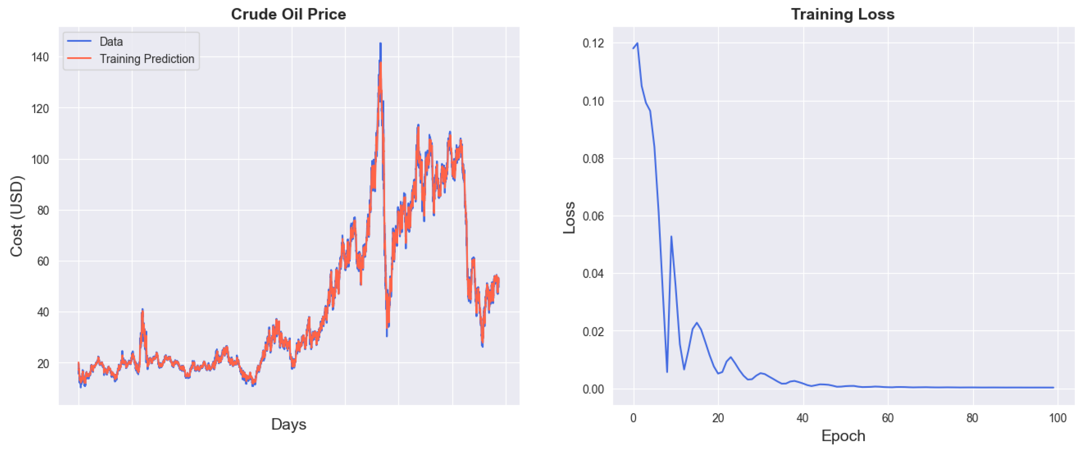
Figure A1.
GBK-Net Training Results.
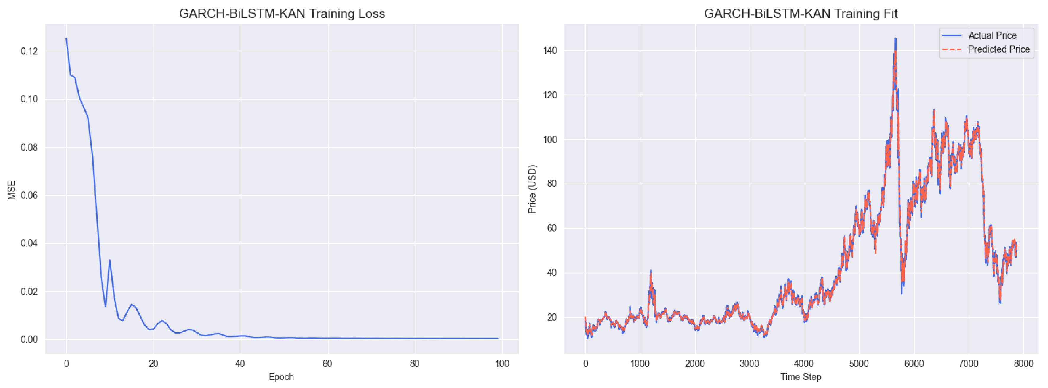
Figure A1 presents the training results of the GARCH–BiLSTM–KAN model. The left panel shows the training loss curve, where the mean squared error (MSE) loss declines rapidly within the first 20 epochs and stabilizes around 0.025 after 60 epochs over 100 training iterations, indicating efficient convergence. The right panel displays the training fit comparison, with the predicted prices (red line) closely aligning with the actual prices (blue line) across time steps 0–8000, demonstrating the model’s robust fitting capability on the training dataset, effectively capturing both overall trends and local fluctuations in crude oil prices. This design is rooted in the Kolmogorov superposition theorem and spline approximation theory [39,65].
Simultaneously, the volatility information provided by GARCH belongs to the "basic feature layer" and is not the final prediction basis.Even if the conditional normal distribution has a bias in the initial portrayal of extreme volatility, the subsequent BiLSTM and KAN modules are able to correct for this bias by means of "time series correlation capture" and "nonlinear refinement". Consequently, using the "multi-component synergy" to avoids the limitations inherent in a single distributional assumption.
Figure A2.
CNN–LSTM–KAN Training Results.
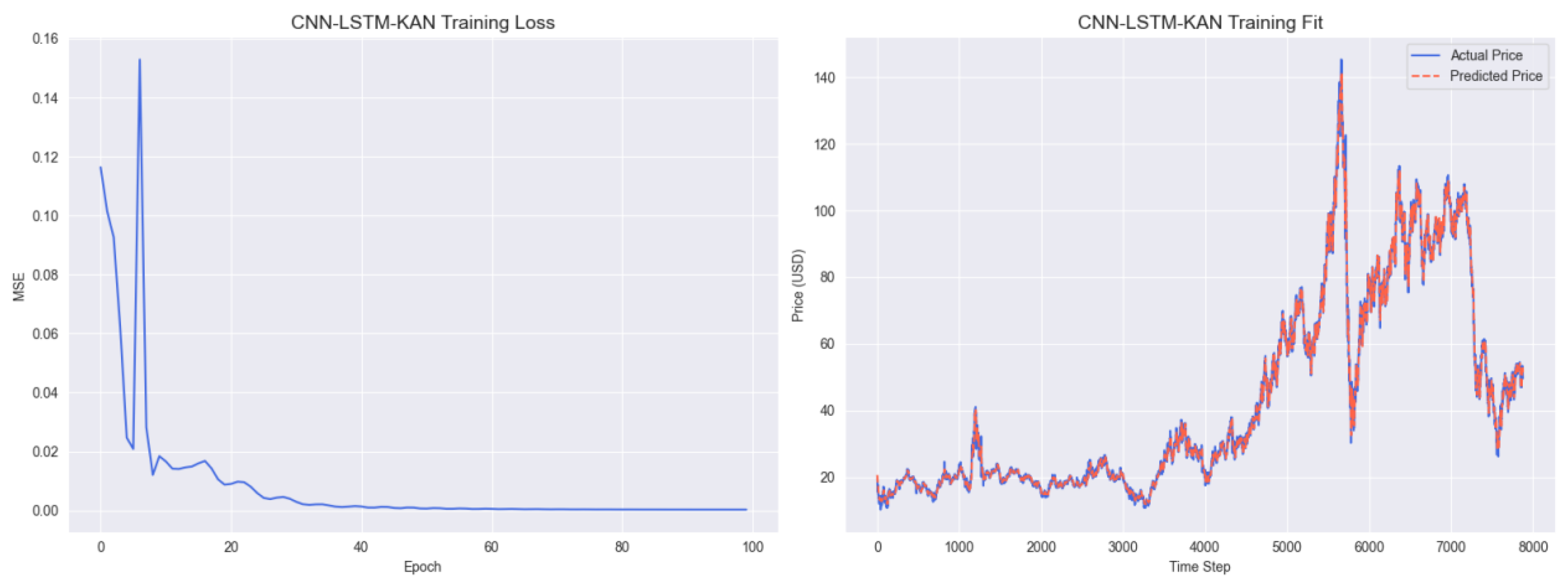
Figure A2 illustrates the training performance of the hybrid CNN–LSTM–KAN model. The left panel presents the training loss curve, which decreases steadily during the first 70 epochs before stabilizing around 0.04 thereafter. This final loss value is higher than that of the GARCH–BiLSTM–KAN model and indicates relatively slower convergence compared with its counterpart. The right panel shows that the predicted prices (green line) generally follow the actual prices (blue line). However, minor deviations occur during periods of heightened volatility (e.g., 2008 and 2020), indicating a weaker ability to capture extreme market fluctuations compared with the GARCH–BiLSTM–KAN model.
Figure A3.
CNN-LSTM Training Results.
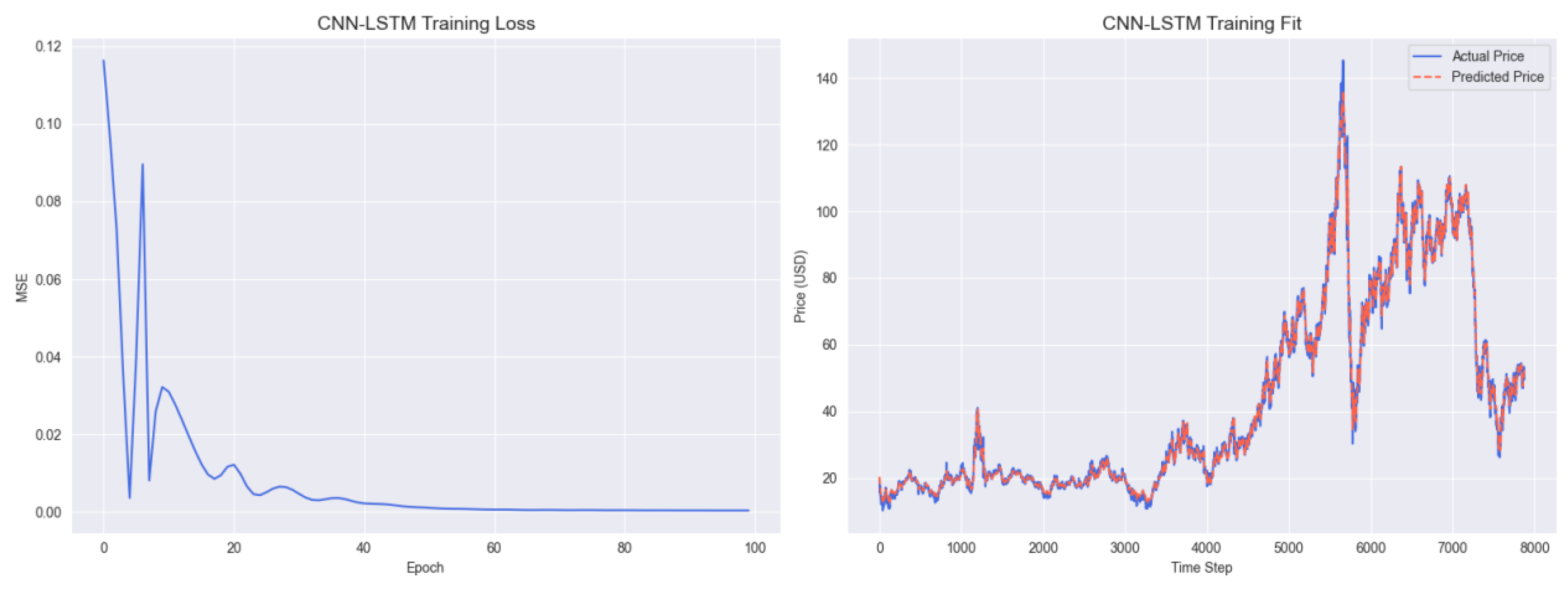
Figure A3 displays the training results of the CNN-LSTM model. The left training loss curve shows a slow decline in loss, stabilizing around 0.06 after 80 epochs, indicating less efficient learning compared to models integrated with KAN. The right panel demonstrates that the predicted prices (orange line) exhibit noticeable lags behind the actual prices (blue line) during sharp price changes (e.g., the 2014–2016 oil crash), highlighting limitations in capturing nonlinear temporal dependencies.
Figure A4.
LSTM Training Results.
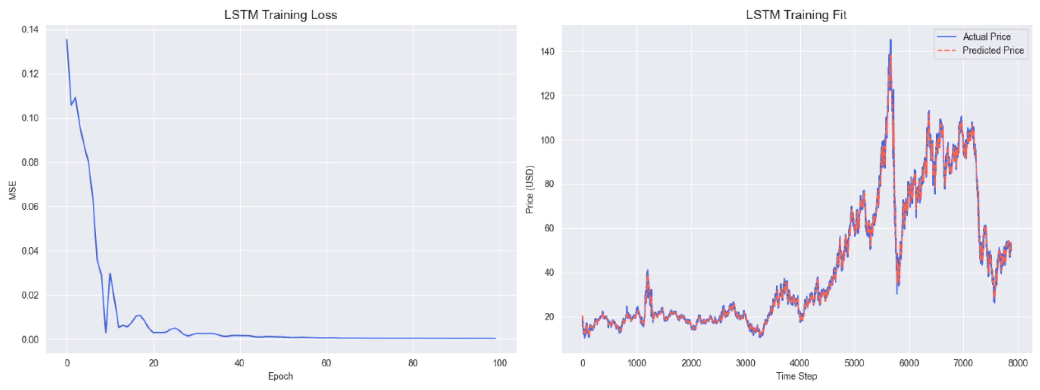
Figure A4 presents the training process of the standalone LSTM model. The left training loss curve remains relatively high, stabilizing around 0.10 after 100 epochs, confirming the inadequacy of unidirectional sequence learning in volatility modeling. The right panel shows significant deviations between the predicted prices (purple line) and actual prices (blue line) during high-volatility periods, reflecting the model’s inability to account for volatility clustering.
Figure A5.
LSTM-KAN Training Results.
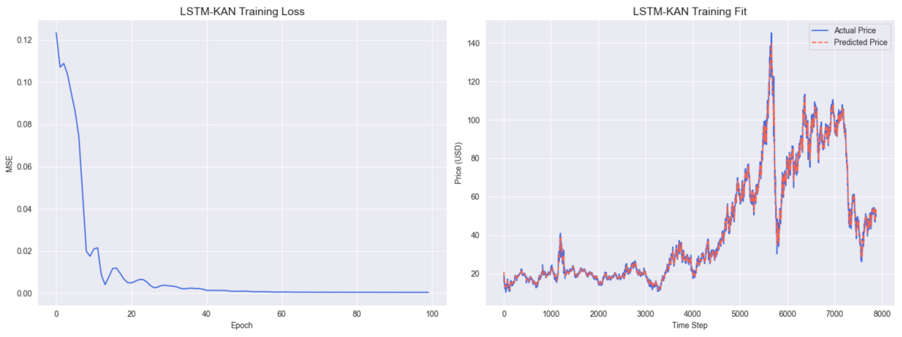
Figure A5 shows the training performance of the LSTM-KAN hybrid model. The left training loss curve decreases to around 0.08 after 100 epochs, slightly lower than that of the standalone LSTM but higher than GARCH–BiLSTM–KAN, indicating that KAN alone cannot fully compensate for the lack of volatility modeling. The right panel reveals that while the predicted prices (yellow line) show moderate alignment with actual prices, they fail to capture abrupt price shifts (e.g., the 2020 COVID–19 crash), demonstrating the need for bidirectional temporal learning.
Figure A6.
GARCH-LSTM Training Results.
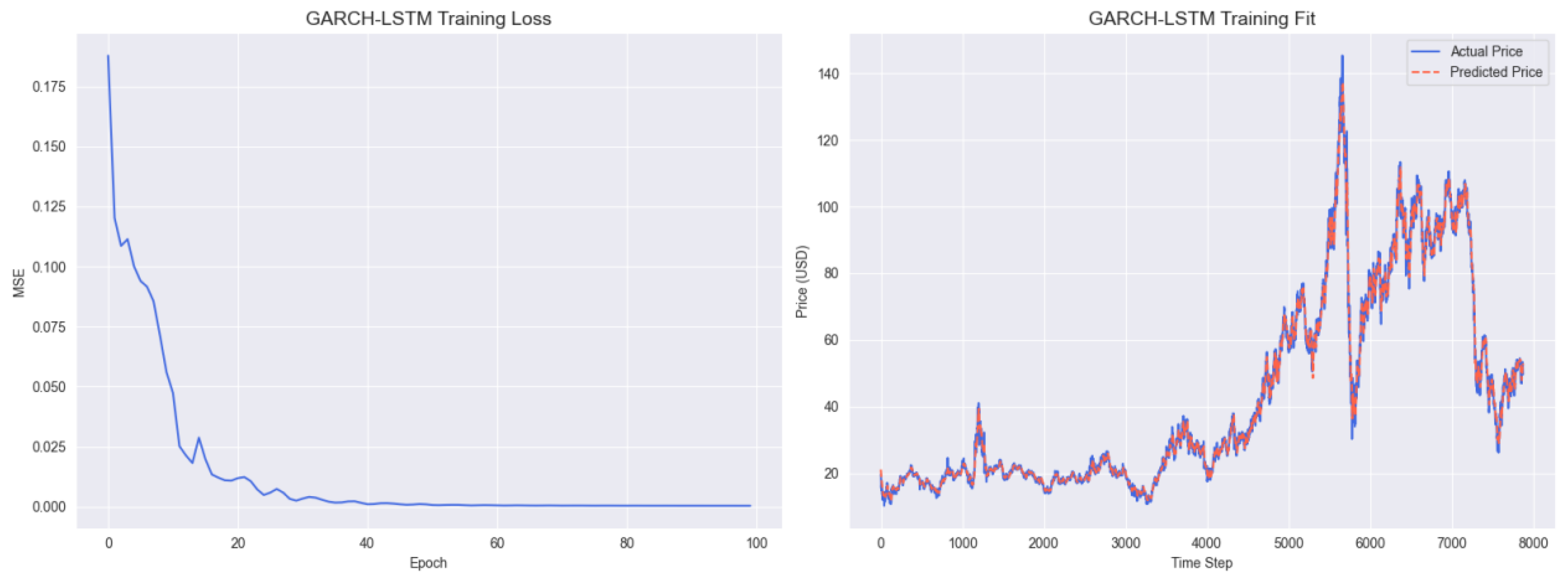
Figure A6 illustrates the training results of the GARCH-LSTM hybrid model. The left training loss curve stabilizes around 0.075 after 90 epochs, higher than that of GARCH–BiLSTM–KAN, indicating that the unidirectional LSTM structure limits the model’s ability to capture bidirectional temporal dependencies. The right panel shows that the predicted prices (gray line) exhibit larger errors compared to actual prices during the post-2020 recovery period, highlighting the superiority of bidirectional learning (BiLSTM) in capturing asymmetric price dynamics, particularly in trend during market recovery phases.
Table A2.
Diebold-Mariano tests: GBK-Net vs. Competitors
| Competitor | Mean Loss Difference | DM Statistic | p-value |
|---|---|---|---|
| EGARCH | |||
| GARCH | |||
| GARCH-LSTM | |||
| LSTM-KAN | |||
| LSTM | |||
| CNN-LSTM | |||
| CNN–LSTM–KAN |
Note: In the test, the lag order is set to 5 to adapt to the autocorrelation characteristics of financial time series. The loss difference is calculated based on the true values and predicted values of the test set to ensure no leakage of time series data. The results support that the accuracy advantage of GBK-Net in this task is statistically significant.
Table A2 presents Diebold-Mariano (DM) test results verifying prediction accuracy differences between GBK-Net and benchmarks like EGARCH/GARCH (using squared loss for MSE-based error measurement). Defined as
, the loss difference sequence, paired with Newey-West HAC standard errors for one-sided testing, shows consistently negative mean differences. All p-values are well below , and negative t-statistics reject the "no accuracy difference" null hypothesis. Thus, within tested tasks/scenarios, GBK-Net outperforms benchmarks significantly, with its multi-feature, bidirectional temporal architecture excelling in pattern mining and fluctuation characterization, validated by statistical tests.
Appendix B. Robustness to Return Definitions
We replicate the main experiments using arithmetic returns as the target instead of shifted log-returns. Price targets are reconstructed via (24). Across all models, the relative ranking remains unchanged and the metric deltas are minor, confirming that our conclusions are not sensitive to the choice of return definition.
References
- Clark, T.E.; West, K.D. Approximately Unbiased Tests of Equal Predictive Accuracy in Nested Models. Journal of Econometrics 2007, 138, 291–311. [CrossRef]
- Hamilton, J.D. Oil and the Macroeconomy since World War II. Journal of Political Economy 1983, 91, 228–248. [CrossRef]
- Kilian, L. Not All Oil Price Shocks Are Alike: Disentangling Demand and Supply Shocks in the Crude Oil Market. American Economic Review 2009, 99, 1053–1069. [CrossRef]
- Safari, A.; Davallou, M. Oil price forecasting using a hybrid model. Energy 2018, 148, 49–58. [CrossRef]
- Pindyck, R.S. Volatility and commodity price dynamics. Journal of Futures Markets 2004, 24, 1029–1047. [CrossRef]
- Alquist, R.; Kilian, L.; Vigfusson, R.J. Forecasting the Price of Oil. In Handbook of Economic Forecasting; Elliott, G.; Timmermann, A., Eds.; Elsevier, 2013; Vol. 2, pp. 427–507.
- Barsky, R.B.; Kilian, L. Oil and the Macroeconomy since the 1970s. Journal of Economic Perspectives 2004, 18, 115–134. [CrossRef]
- Mork, K.A. Oil and the Macroeconomy When Prices Go Up and Down: An Extension of Hamilton’s Results. Journal of Political Economy 1989, 97, 740–744. [CrossRef]
- Kilian, L.; Park, C. The Impact of Oil Price Shocks on the U.S. Stock Market. International Economic Review 2009, 50, 1267–1287. [CrossRef]
- Edelstein, P.; Kilian, L. How Sensitive are Consumer Expenditures to Retail Energy Prices? Journal of Monetary Economics 2009, 56, 766–779. [CrossRef]
- Baumeister, C.; Kilian, L. Real-Time Forecasts of the Real Price of Oil. Journal of Business & Economic Statistics 2012, 30, 326–336. [CrossRef]
- Zhang, D. Oil shocks and stock markets revisited: Measuring connectedness from a global perspective. Energy Economics 2017, 62, 323–333. [CrossRef]
- Atif, M.; Rabbani, M.R.; Bawazir, H.; Hawaldar, I.T.; Chebab, D.; Karim, S.; AlAbbas, A. Oil price changes and stock returns: Fresh evidence from oil exporting and oil importing countries. Cogent Economics & Finance 2022, 10, 2018163. [CrossRef]
- Gupta, R.; Pierdzioch, C.; Salisu, A.A. Oil-price uncertainty and the UK unemployment rate: A forecasting experiment with random forests using 150 years of data. Resources Policy 2022, 77, 102662. [CrossRef]
- Kilian, L.; Murphy, D.P. The role of inventories and speculative trading in the global market for crude oil. Journal of Applied Econometrics 2014, 29, 454–478. [CrossRef]
- Hegerty, S.W. Commodity-price volatility and macroeconomic spillovers: Evidence from nine emerging markets. The North American Journal of Economics and Finance 2016, 35, 23–37. [CrossRef]
- Hamilton, J.D. Nonlinearities and the macroeconomic effects of oil prices. Macroeconomic Dynamics 2011, 15, 364–378. [CrossRef]
- Bollerslev, T.; Chou, R.Y.; Kroner, K.F. ARCH modeling in finance: A review of the theory and empirical evidence. Journal of Econometrics 1992, 52, 5–59. [CrossRef]
- Engle, R.F. Autoregressive conditional heteroscedasticity with estimates of the variance of United Kingdom inflation. Econometrica 1982, 50, 987–1007. [CrossRef]
- Kim, H.Y.; Won, C.H. Forecasting the volatility of stock price index: A hybrid model integrating LSTM with multiple GARCH-type models. Expert Systems with Applications 2018, 103, 25–37. [CrossRef]
- Nelson, D.B. Conditional Heteroskedasticity in Asset Returns: A New Approach. Econometrica 1991, 59, 347–370. [CrossRef]
- Glosten, L.R.; Jagannathan, R.; Runkle, D.E. On the Relation between the Expected Value and the Volatility of the Nominal Excess Return on Stocks. The Journal of Finance 1993, 48, 1779–1801. [CrossRef]
- Zakoïan, J.M. Threshold Heteroskedastic Models. Journal of Economic Dynamics and Control 1994, 18, 931–955. [CrossRef]
- Parzen, E. ARARMA models for time series analysis and forecasting. Journal of Forecasting 1982, 1, 67–82. [CrossRef]
- Hyndman, R.J.; Athanasopoulos, G. Forecasting: Principles and Practice, 2 ed.; OTexts, 2018.
- Bollerslev, T. Generalized autoregressive conditional heteroskedasticity. Journal of Econometrics 1986, 31, 307–327. [CrossRef]
- Engle, R. GARCH 101: The use of ARCH/GARCH models in applied econometrics. Journal of Economic Perspectives 2001, 15, 157–168. [CrossRef]
- Silvennoinen, A.; Teräsvirta, T. Multivariate GARCH Models. In Handbook of Financial Time Series; Andersen, T.G.; Davis, R.A.; Kreiss, J.P.; Mikosch, T., Eds.; Springer: Berlin, Heidelberg, 2009; pp. 201–229.
- Cortes, C.; Vapnik, V. Support-vector networks. Machine Learning 1995, 20, 273–297. [CrossRef]
- Breiman, L. Random forests. Machine Learning 2001, 45, 5–32. [CrossRef]
- Hochreiter, S.; Schmidhuber, J. Long short-term memory. Neural Computation 1997, 9, 1735–1780. [CrossRef] [PubMed]
- Fischer, T.; Krauss, C. Deep learning with long short-term memory networks for financial market predictions. European Journal of Operational Research 2018, 270, 654–669. [CrossRef]
- Schuster, M.; Paliwal, K.K. Bidirectional recurrent neural networks. IEEE Transactions on Signal Processing 1997, 45, 2673–2681. [CrossRef]
- Yang, K.; Hu, N.; Tian, F. Forecasting Crude Oil Volatility Using the Deep Learning-Based Hybrid Models With Common Factors. Journal of Futures Markets 2024, 44, 1429–1446. [CrossRef]
- Hu, Z. Crude oil price prediction using CEEMDAN and LSTM-attention with news sentiment index. Oil & Gas Science and Technology – Revue d’IFP Energies nouvelles 2021, 76, 28. [CrossRef]
- Li, Y.; Dai, W. Bitcoin price forecasting method based on CNN-LSTM hybrid neural network model. The Journal of Engineering 2020, pp. 344–347.
- Liu, Z.; Wang, Y.; Vaidya, S.; Ruehle, F.; Halverson, J.; Soljačić, M.; Tegmark, M. KAN: Kolmogorov-Arnold Networks, 2024. arXiv:2404.19756.
- Kingma, D.P.; Ba, J. Adam: A Method for Stochastic Optimization. International Conference on Learning Representations 2015.
- Kolmogorov, A.N. On the Representation of Continuous Functions of Many Variables by Superposition of Continuous Functions of One Variable and Addition. Doklady Akademii Nauk SSSR 1957, 114, 953–956.
- Lin, Y.; Wang, M.; Xu, L.; Zhang, F. The maximum forcing number of a polyomino. Australas. J. Combin 2017, 69, 306–314.
- Wang, M.; Yang, W.; Wang, S. Conditional matching preclusion number for the Cayley graph on the symmetric group. Acta Math. Appl. Sin.(Chinese Series) 2013, 36, 813–820.
- Wang, M.; Lin, Y.; Wang, S. The connectivity and nature diagnosability of expanded k-ary n-cubes. RAIRO-Theoretical Informatics and Applications-Informatique Théorique et Applications 2017, 51, 71–89. [CrossRef]
- Wang, S.; Wang, M. A Note on the Connectivity of m-Ary n-Dimensional Hypercubes. Parallel Processing Letters 2019, 29, 1950017. [CrossRef]
- Wang, S.; Zhao, L.; Wang, S. Fault-tolerant strong Menger connectivity with conditional faults on wheel networks. Discret. Appl. Math. 2025, 371, 115–126. [CrossRef]
- Wang, M.; Ren, Y.; Lin, Y.; Wang, S. The tightly super 3-extra connectivity and diagnosability of locally twisted cubes. American Journal of Computational Mathematics 2017, 7, 127–144. [CrossRef]
- Wang, M.; Lin, Y.; Wang, S.; Wang, M. Sufficient conditions for graphs to be maximally 4-restricted edge connected. Australas. J Comb. 2018, 70, 123–136.
- Wang, S.; Wang, Y.; Wang, M. Connectivity and matching preclusion for leaf-sort graphs. Journal of Interconnection Networks 2019, 19, 1940007. [CrossRef]
- Zhao, L.; Wang, S. Structure connectivity and substructure connectivity of split-star networks. Discret. Appl. Math. 2023, 341, 359–371. [CrossRef]
- Goodfellow, I.; Bengio, Y.; Courville, A. Deep Learning; MIT Press: Cambridge, MA, 2016.
- Pindyck, R.S. Volatility in natural gas and oil markets. Journal of Energy and Development 2004, 30, 1–.
- Khan, N.; Fahad, S.; Naushad, M.; Faisal, S. COVID-2019 locked down effects on oil prices and its effects on the world economy. SSRN working paper, 2020. SSRN No. 3588810.
- Yergin, D. The Quest: Energy, Security, and the Remaking of the Modern World; Penguin Press: New York, 2011.
- Hamilton, J.D. Causes and Consequences of the Oil Shock of 2007–08. NBER Working Paper 15002, National Bureau of Economic Research, 2009.
- Baumeister, C.; Kilian, L. Forty Years of Oil Price Fluctuations: Why the Price of Oil May Still Surprise Us. Journal of Economic Perspectives 2016, 30, 139–160. [CrossRef]
- Ghorbel, A.; Jeribi, A. Contagion of COVID-19 pandemic between oil and financial assets: evidence of multivariate Markov switching GARCH models. Journal of Investment Compliance 2021, 22, 151–169. [CrossRef]
- Wang, S.; Wang, Z.; Wang, M.; Han, W. g-Good-neighbor conditional diagnosability of star graph networks under PMC model and MM* model. Frontiers of Mathematics in China 2017, 12, 1221–1234. [CrossRef]
- Wang, M.; Wang, S. Diagnosability of Cayley graph networks generated by transposition trees under the comparison diagnosis model. Ann. of Appl. Math 2016, 32, 166–173.
- Wang, M.; Xiang, D.; Wang, S. Connectivity and diagnosability of leaf-sort graphs. Parallel Processing Letters 2020, 30, 2040004. [CrossRef]
- Lim, B.; Arik, S.Ö.; Loeff, N.; Pfister, T. Temporal Fusion Transformers for Interpretable Multi-horizon Time Series Forecasting. International Journal of Forecasting 2021, 37, 1748–1764. [CrossRef]
- Zhou, G.; Wang, R.F. The Heterogeneous Network Community Detection Model Based on Self-Attention. Symmetry 2025, 17. [CrossRef]
- Yang, Z.X.; Li, Y.; Wang, R.F.; Hu, P.; Su, W.H. Deep Learning in Multimodal Fusion for Sustainable Plant Care: A Comprehensive Review. Sustainability 2025, 17, 5255. [CrossRef]
- Wang, R.F.; Qu, H.R.; Su, W.H. From Sensors to Insights: Technological Trends in Image-Based High-Throughput Plant Phenotyping. Smart Agricultural Technology 2025, p. 101257.
- Wang, Z.; Zhang, H.W.; Dai, Y.Q.; Cui, K.; Wang, H.; Chee, P.W.; Wang, R.F. Resource-Efficient Cotton Network: A Lightweight Deep Learning Framework for Cotton Disease and Pest Classification. Plants 2025, 14, 2082. [CrossRef]
- Yang, Z.Y.; Xia, W.K.; Chu, H.Q.; Su, W.H.; Wang, R.F.; Wang, H. A comprehensive review of deep learning applications in cotton industry: From field monitoring to smart processing. Plants 2025, 14, 1481. [CrossRef] [PubMed]
- de Boor, C. A Practical Guide to Splines; Springer: New York, 1978.
| 1 | Periods of high volatility are often followed by high volatility, and low volatility tends to persist. |
| 2 | The assumption that the variance of error terms is constant over time. |
| 3 | |
| 4 |
Figure 1.
Overall framework of the GARCH–BiLSTM–KAN (GBK-Net) hybrid model.
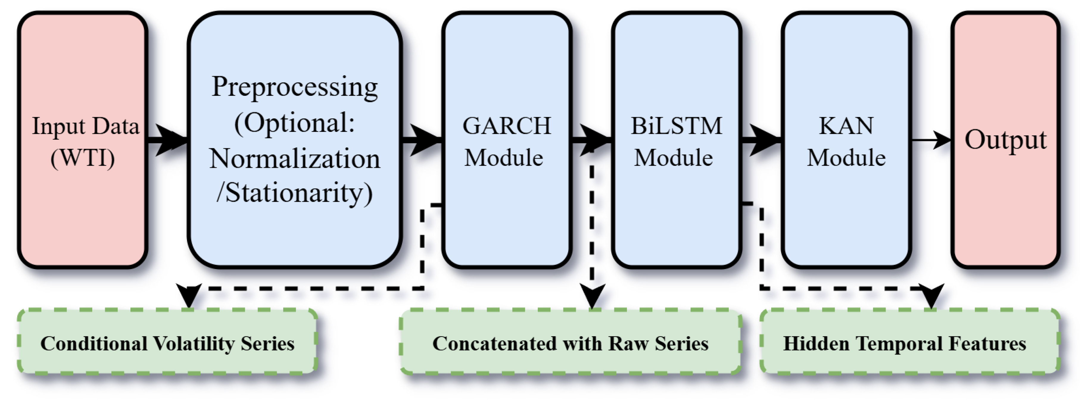
Figure 2.
Schematic Diagram of Hidden State Fusion Process in BiLSTM
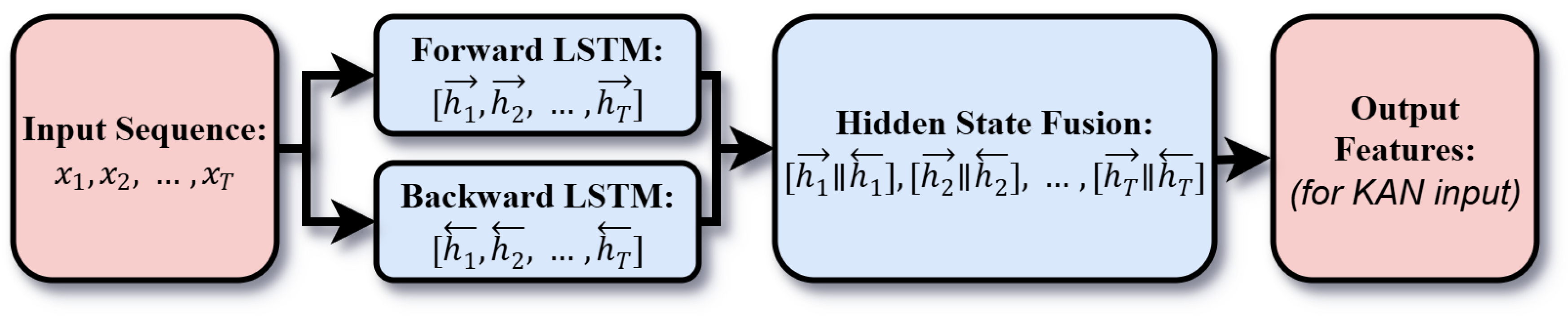
Figure 3.
Schematic Diagram of the KAN Model Structure
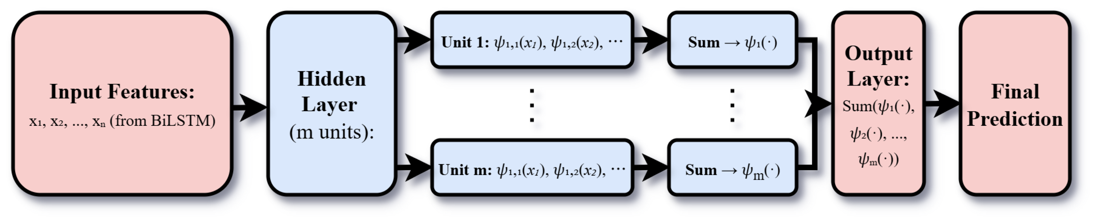
Figure 4.
Trend Chart of WTI Crude Oil Prices from 1986 to 2025
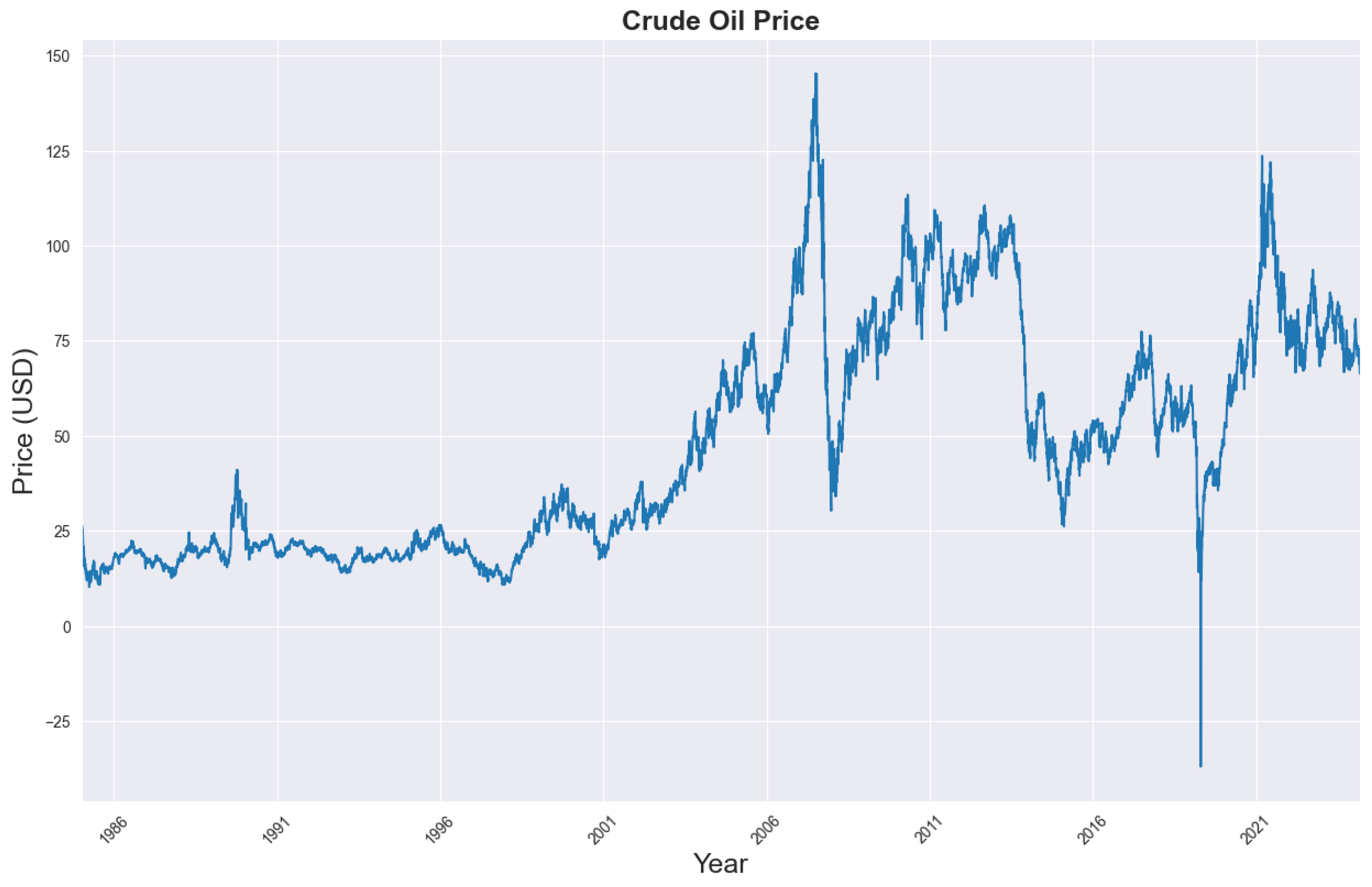
Figure 5.
Trend Chart of the First Difference of WTI Crude Oil Prices
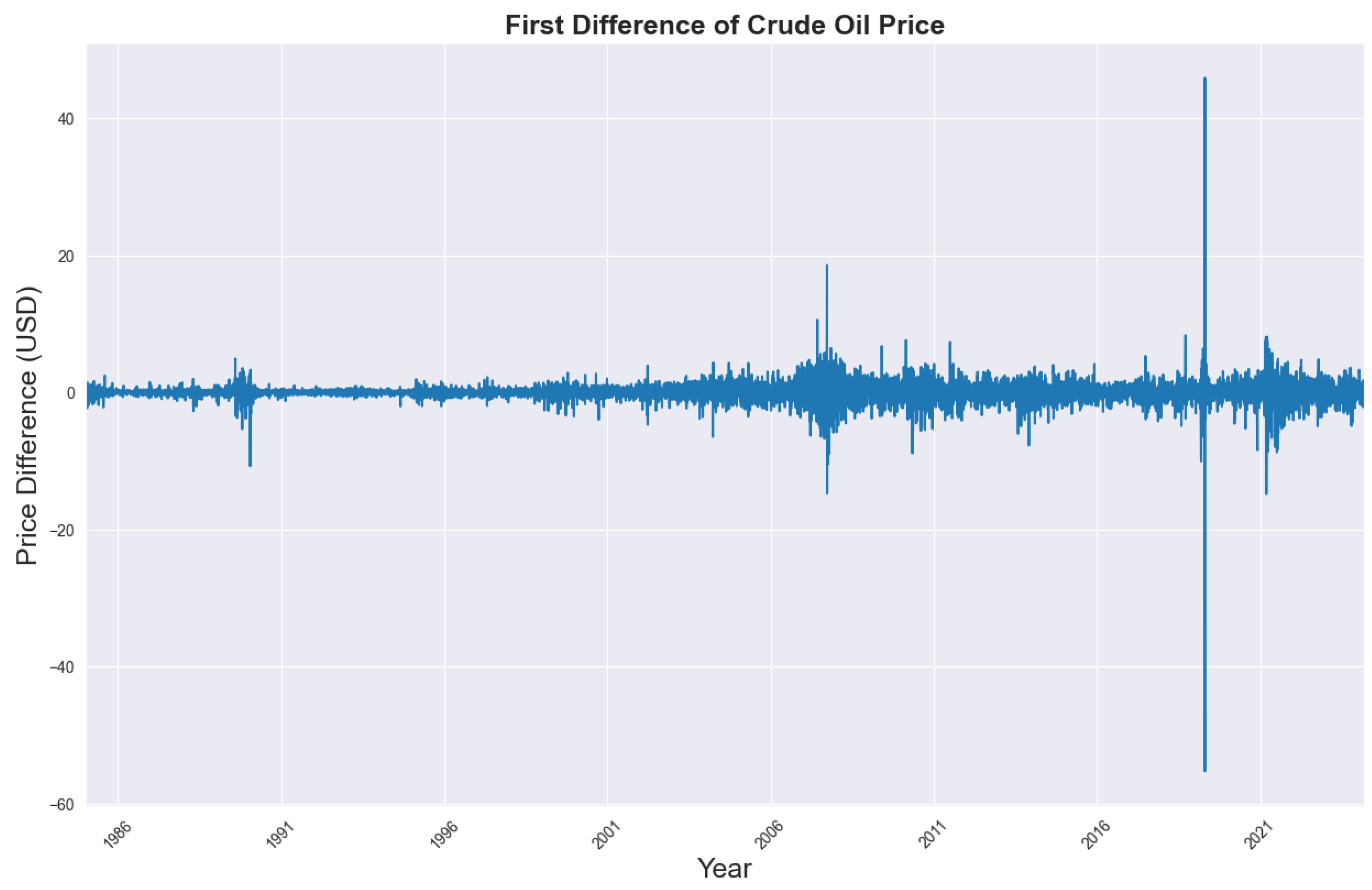
Figure 9.
Training Loss Comparison Across Models (MSE vs. Epochs)
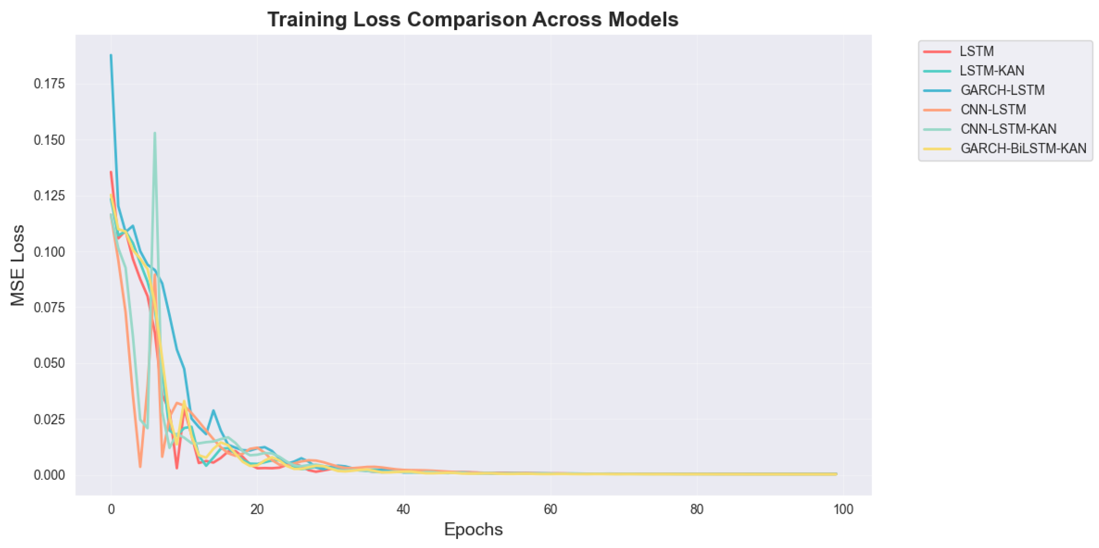
Table 1.
Key Parameters of the GBK-Net Hybrid Model.
| Component | Key Parameters | Values |
|---|---|---|
| GARCH | Order | (1,1) |
| Distribution | Conditional Normal | |
| BiLSTM | Hidden Units (per direction) | 32 |
| Number of Layers | 2 | |
| Optimizer | Adam | |
| Learning Rate | 0.01 | |
| KAN | Basis Functions | Cubic B-splines (5 knots) |
| Width Structure | [64,1] | |
| Optimizer | Adam | |
| Learning Rate | 0.01 | |
| Training | Loss Function | MSE |
| Epochs | 100 | |
| Lookback Window | 20 (Among 10/20/30/40, 20 has the lowest RMSE) |
|
| Evaluation Metrics | Primary Metrics | RMSE, MAE, |
| Train-Test Split | 80%–20% | |
| Feature Scaling | MinMaxScaler () |
Table 2.
Descriptive Statistics of WTI Crude Oil Prices (1986–2025).
| Statistic | Count | Mean | Std | Min | 25% | 50% | 75% | Max |
|---|---|---|---|---|---|---|---|---|
| Value | 9,866 | 47.73 | 29.64 | -36.98 | 20.22 | 40.69 | 71.47 | 145.31 |
Table 3.
Performance Metrics of Various Models on the Test Set.
| Model | RMSE | MAE | |
|---|---|---|---|
| GBK-Net | 2.4876 | 1.5156 | 0.9810 |
| CNN–LSTM–KAN | 2.6047 | 1.6464 | 0.9792 |
| CNN-LSTM | 2.7639 | 1.7693 | 0.9765 |
| LSTM | 2.8802 | 1.8445 | 0.9745 |
| LSTM-KAN | 2.9223 | 1.8780 | 0.9738 |
| GARCH-LSTM | 3.0753 | 1.9996 | 0.9710 |
| GARCH | 4.8921 | 3.2157 | 0.9235 |
| EGARCH | 5.1236 | 3.4589 | 0.9187 |
Table 4.
Performance Metrics of Various Models in Ablation Experiments.
| Model | RMSE | MAE | |
|---|---|---|---|
| GBK-Net | 2.4876 | 1.5156 | 0.9810 |
| GARCH-KAN (Ablated BiLSTM) | 9.2605 | 8.3800 | 0.7367 |
| GARCH-BiLSTM-FC (Ablation of KAN) | 5.0026 | 3.6244 | 0.9232 |
| BiLSTM-KAN (Ablated GARCH) | 3.4220 | 2.4248 | 0.9640 |
Disclaimer/Publisher’s Note: The statements, opinions and data contained in all publications are solely those of the individual author(s) and contributor(s) and not of MDPI and/or the editor(s). MDPI and/or the editor(s) disclaim responsibility for any injury to people or property resulting from any ideas, methods, instructions or products referred to in the content. |
© 2025 by the authors. Licensee MDPI, Basel, Switzerland. This article is an open access article distributed under the terms and conditions of the Creative Commons Attribution (CC BY) license (http://creativecommons.org/licenses/by/4.0/).
Copyright: This open access article is published under a Creative Commons CC BY 4.0 license, which permit the free download, distribution, and reuse, provided that the author and preprint are cited in any reuse.


