
Submitted:
08 July 2025
Posted:
09 July 2025
You are already at the latest version
Abstract
This study presents a novel alternative to the standardized credit risk assessment model currently mandated by Colombia's Superintendence of the Solidarity Economy (SES). Addressing critical limitations of the regulatory model, particularly its reliance on binary variables and limited contextualization of institutional heterogeneity, this study develops and evaluates explainable machine learning (ML) models aligned with the Internal Ratings-Based (IRB) approach under Basel II. The proposed framework integrates continuous behavioral and financial variables with model-agnostic interpretability via SHAP (SHapley Additive exPlanations). Our proposal represents the first empirical application of such techniques within the Colombian solidarity finance sector. The data set comprises over 17,000 individual credit histories, segmented into debit and non-debit loans. Performance evaluation of multiple regression models, including Ridge, Decision Tree, Random Forest, XGBoost, and LightGBM, demonstrated that LightGBM achieves superior accuracy. Beyond predictive gains, the model enables granular interpretability and supports compliance with governance and accountability standards. The results highlight the potential of adaptive machine learning (ML) models to complement regulatory frameworks, enhance credit decision-making, and optimize capital allocation strategies in solidarity-based financial institutions.
Keywords:
credit risk modeling
; explainable machine learning
; internal ratings-based approach
; LightGBM
; SHAP values
1. Introduction
Credit risk management is of fundamental importance in ensuring the stability of financial institutions, as it determines their capacity to absorb losses arising from credit defaults (Jorion, 2000). In this context, international standards, particularly those developed by the Basel Committee on Banking Supervision (2011), have played a pivotal role in the development of regulatory frameworks that guide the identification, measurement, and mitigation of financial risks. The Basel II Accord represented a significant milestone in the field of credit risk modeling, introducing three distinct approaches for this purpose. These were the standardized approach, the foundation internal ratings-based (IRB) approach, and the advanced IRB approach. Each method provides varying degrees of flexibility in estimating the components of expected loss probability of default (PD), loss given default (LGD), and exposure at default (EAD). The capital requirement is uniform for each risk segment under the standardized approach, with external credit ratings serving as the primary determinant of capital requirements. However, it is important to note that financial institutions typically gather extensive information during the origination and monitoring of loans, thereby creating opportunities to develop more granular and accurate credit risk estimates. The IRB approaches introduced under Basel II enable institutions to leverage this additional data to enhance the precision of expected loss modeling. The fundamental distinction between the foundation and advanced IRB methods lies in the degree of autonomy afforded to banks in estimating risk components. While the foundation approach delegates the estimation of LGD and EAD to regulatory authorities, the advanced approach grants full responsibility for these estimates to the institutions themselves. Although implementing advanced methodologies requires considerable investment in infrastructure and analytical capacity, the benefits are substantial. The implementation of more accurate models has been demonstrated to have a dual impact: firstly, it leads to a reduction in excess capital holdings, and secondly, it enhances institutions' ability to manage risk and support sustainable growth.
In the Colombian context, institutions supervised by the Superintendence of the Solidarity Economy (SES) are required to conduct continuous evaluations of the credit risk associated with their loan portfolios. This evaluation is to be conducted at the inception of the loan and regular intervals throughout the credit lifecycle, encompassing all lending modalities (consumer, housing, commercial, and microcredit). In response to the need for tools that enhance credit risk management, various regulatory models and indicators have been developed to analyze credit exposure and estimate default probabilities. It is noteworthy that the SES has developed a Reference Model that serves as a standardized guide for rating credit portfolios and estimating expected losses (Superintendencia de la Economía Solidaria, 2024). However, the model is constrained by its reliance on standardized regulatory frameworks. While these provide common guidelines, they exhibit significant limitations by failing to consider the unique operational, social, and financial characteristics of each solidarity-based entity. Cooperatives, employee funds, and mutual associations operate under heterogeneous dynamics in terms of size, coverage, governance, and member profiles — factors that directly influence their exposure and response to credit risk.
Furthermore, the current regulatory model adopts a generic approach, relying predominantly on binary variables (e.g., default/non-default, presence/absence of collateral). While operationally straightforward, this strategy significantly reduces the explanatory power of the models, limits the use of informative continuous variables (e.g., income, tenure, payment history, or debt level), and hinders the identification of complex patterns associated with default probability. These technical limitations directly impact credit decision-making by preventing a more nuanced assessment of applicants, which can lead to inefficiencies, financial exclusion, or overexposure to risk.
Given this scenario, there is a clear need to advance toward more adaptive and technically robust credit scoring models tailored to the operational realities of each institution. Accordingly, the objective of this research is to apply explainable machine learning models to credit risk rating in the Colombian solidarity sector and to propose an alternative methodology aligned with the principles of the Basel II IRB approach. To this end, the study applies a range of regression models—both linear and tree-based—on a dataset obtained from a cooperative within the solidarity sector. The dataset comprises a time series of 17,518 members constructed through the integration of monthly files containing relevant credit risk variables. Model performance was assessed using Root Mean Squared Error (RMSE) and the Coefficient of Determination (R²), which respectively measure prediction accuracy and explanatory power. Among the algorithms compared, LightGBM achieved the best performance, minimizing prediction error and yielding a superior R² value.
To ensure the interpretability of results, the SHAP (SHapley Additive exPlanations) technique was applied to identify the specific contribution of each variable to individual predictions. The findings demonstrate that models using continuous variables drawn from real institutional data can produce credit scores comparable to those generated by the SES regulatory model. Additionally, linear models were found capable of achieving acceptable accuracy levels using a reduced set of variables, thereby contributing to transparency and simplicity in the estimation process. LightGBM outperformed traditional linear models, such as Ridge regression, due to its superior ability to capture nonlinear relationships between variables. The SHAP analysis facilitates the interpretation of LightGBM-generated risk ratings, enabling cooperatives to identify the most influential risk factors based on real-time data and communicate them effectively to members, executives, regulators, and supervisory bodies. This interpretability, combined with high predictive performance, positions LightGBM as not only a technically sound alternative but also a governance-aligned tool that fulfills traceability and accountability standards required in modern risk management systems.
The remainder of the article is organized as follows: Section 2 presents the dataset, outlines the regulatory model used in the Colombian solidarity sector, and provides a brief introduction to the machine learning models employed. Section 3 evaluates the predictive performance of the models—regularized linear regression (Ridge), decision trees, random forests, and LightGBM—and analyzes the contribution of each variable to the prediction of default. Section 4 provides a brief discussion of recent regulatory reforms in the Colombian solidarity sector, illustrating how the proposed models align with the logic of the 2025 regulatory changes. Section 5 presents the conclusions.
2. Literature Review
Credit risk management is a fundamental process by which an entity evaluates, grants, and monitors the loans granted to its customers. This process is key to minimizing financial risks and ensuring the stability of the system (Zaragoza, 2018). Therefore, it is necessary to incorporate new techniques that contribute to its mitigation (Paucar, 2022). In this context, the use of Machine Learning (ML) models in the financial sector has gained relevance due to their predictive capabilities. These models have enabled the improvement of credit risk assessment methodologies, the optimization of processes, and the making of more informed decisions based on the results obtained (Castro, 2022).
In contrast, conventional credit risk scoring models, widely used in traditional banking, currently employ advanced techniques to calculate credit risk. These models typically integrate machine learning tools, such as neural networks and random forests, to improve predictive accuracy (Gatla, 2023). However, the complexity of these models often poses challenges in terms of interpretability and transparency, crucial aspects for regulation and user trust. (Yusheng, 2024).
As in banking, credit risk assessment in cooperatives and similar entities presents unique challenges due to their structure and objectives (Bussmann, Giudici, Marinelli, & Papenbrock, 2021). The integration of financial technologies (FinTech) and the use of alternative data are rapidly transforming credit risk assessment methodologies, offering new opportunities to improve accuracy and efficiency (Libda, 2024). Furthermore, the relationship between credit risk models and regulatory capital requirements, particularly in the context of the Basel Accords, highlights the importance of accuracy and comparability in these models (Jackson, 2020).
(Freire, 2024), developed various credit risk classification models using Machine Learning algorithms to evaluate their effectiveness in predicting defaults in a financial institution. To achieve this, he applied logistic regression models, both linear and nonlinear, which were optimized using Newton's method. The results showed that these tools can expedite decision-making related to loan granting and reduce the likelihood of default. For his part, Vasquez (2025) carried out a comparative analysis of Machine Learning algorithms to predict the delinquency of customers affiliated with the financial institution San Francisco de Mocupe. Similarly, Grau (2020) proposed measuring mortgage credit risk using Machine Learning techniques, applying logistic regression, decision trees, and Gradient Boosting to a line of mortgage loans to determine which model offered a more efficient analysis from a business perspective.
On the other hand, Valenzuela and R (2024) conducted a study aimed at identifying the most widely used and effective Machine Learning algorithms for credit risk management in the Peruvian financial system. In this analysis, several algorithms were compared, including decision trees, Support Vector Machines (SVMs), Random Forests, neural networks, Naive Bayes, K-nearest neighbors (KNNs), and logistic regression, among others. The results indicated that decision trees and SVM were the most effective in predicting payment defaults and managing credit risk among the analyzed entities. On the other hand, (Gonzalez and Coveñas de León) developed a credit scoring model using alternative data and artificial intelligence, implementing techniques such as XGBoost, logistic regression, and Random Forest to demonstrate the effectiveness of unconventional data in assessing credit risk.
Authors such as Machado and Karray (2022) investigate the use of hybrid machine learning models to improve the prediction of credit scores for commercial customers, utilizing data from a large US bank. They first group clients using unsupervised algorithms (k-Means and DBSCAN) and then apply supervised regression models, such as AdaBoost, Gradient Boosting, SVM, Decision Tree, Random Forest, and Neural Networks. The results show that hybrid models outperform individual models, especially those that combine k-Means with Decision Tree or Random Forest. Additionally, including historical credit score data enhances accuracy. The best individual models were RF, DT, and GB, while ANN had the worst performance.
In conclusion, hybrid models are more effective because pre-clustering reduces dimensionality and enhances prediction accuracy. (Gambacorta, Huang, Qiu, & Wang, 2024) Compare machine learning (ML) models with traditional statistical methodologies to predict credit losses and defaults using data from a leading fintech in China. The study evaluates three models: one based on machine learning (Model I), another using traditional variables (Model II), and a third that combines traditional and non-traditional variables (Model III). The data includes credit card information and users' digital activity. The results show that the ML model (Model I) outperforms the others in predictive capacity and stability, even in the face of a regulatory shock. The use of non-traditional data and machine learning (ML) techniques significantly improves accuracy. Although performance improves with a longer customer-bank relationship, the advantage of the ML model diminishes overtime. In conclusion, ML models are more accurate and resilient in the face of economic or regulatory changes, especially useful for evaluating customers with a low credit history.
Finally, Donovan, Jennings, Koharki, and Lee (2021) propose a new measure of credit risk, known as the TCR Score, which is based on qualitative information extracted from transcripts of conference calls and the Management Discussion and Analysis (MD&A) sections of annual reports. They utilize supervised machine learning (SVR, sLDA, and Random Forest) to correlate the language used in these disclosures with CDS spreads, thereby generating a continuous numerical measure of credit risk. The results show that the TCR Score is a better predictor of various future credit events (such as bankruptcies, downgrades, and price shocks) than traditional measures. Conference calls are especially useful for capturing the variation in risk within a company over time, while MD&A focuses more on differences between companies. Overall, the study demonstrates that narrative language contains valuable information that can enhance credit risk measurement, particularly in companies without traditional public measures.
3. Materials and Methods
3.1. Data Construction
The database used in this study comprises a total of 701,760 records and was constructed using proprietary information provided by a Colombian savings and credit cooperative within the solidarity-based financial sector. The dataset corresponds to a time series of 17,518 individual members and was generated through the systematic integration of multiple monthly files containing variables relevant to credit risk analysis. Specifically, 37 files corresponding to the individual credit portfolio reports were consolidated, covering the 36 months preceding the evaluation date as well as the evaluation month itself. In addition to the credit portfolio reports, the data integration process incorporated auxiliary files detailing information on members, employees, and debtors associated with the sale of goods and services, as well as the individual savings report and the individual member contributions report. In total, 40 different reports were merged into a unified data structure. The integration was executed using the unique loan identification number as the relational key across files, ensuring both consistency and data integrity throughout the process. The compiled data pertains exclusively to consumer loans, including both credit with debit and credit without debit, spanning an approximate three-year timeframe. For modeling purposes, the consolidated dataset was segmented into two distinct files: one corresponding to credits with debit consumer loans, comprising 6,660 records, and another for credits non-debit consumer loans, encompassing 10,858 records. Although the raw database initially included 96 variables, the selection of predictive features for the non-debit credits was guided by the 12 variables specified in the official regulatory model, as detailed in Appendix A. This methodological approach ensured both regulatory alignment and relevance in the construction of predictive models.
3.2. Regulatory Reference Model
This section presents the regulatory model proposed by the Superintendence of the Solidarity Economy (SES) for estimating credit risk ratings, as applied to both non-debit and debit consumer credit portfolios. (Superintendencia de la Economia Solidaria, 2024).
3.2.1. Regulatory Model in the Solidarity Sector: Non-Debit Consumer Credit Portfolio
Z= - 1.8017 – 0.3758 × EA – 1.1475 × AP + 0.4934 × REEST – 0.387 × CUENAHO – 1.0786 × CDAT – 0.0167 × PER + 0.3204 × ENTIDAD1 – 0.8419 × SALPRES +0.1271 × ANTIPRE1 – 0.3912 × ANTIPRE2 – 0.4892 × VIN2 + 0.7877 × MORA1230+ 2.5651 × MORA1260 + 0.696 × MORA2430 + 2.908 × MORA2460 + 0.8114 × MORA3615
3.2.2. Regulatory Model in the Solidarity Sector: Debit Consumer Credit Portfolio
Z = - 2.2504 – 0.8444 × EA- 1.0573 × AP + 1.0715 × T C – 1.3854 × COOC DAT + 0.7833 × ANTIPRE1 + 0.8526 × MORA15 + 1.4445 × MORA1230 + 1.3892 × MORA1260 + 0.2823 × MORA2430 + 0.7515 × MORA2460 – 0.6632 × SIN MORA + 1.2362 × MORTRIM
3.3. Proposed Models
Figure 1 shows the project workflow. We split the entire dataset into two sets: a training set and a testing set. We implemented a k-fold cross-validation to tune the hyperparameters of the regression models. The cross-validation also allowed us to validate the variability of the model's prediction for different training datasets. A randomized search function was used to perform the hyperparameter tuning by trying random combinations (in a defined range) instead of testing all possibilities.
Once the model is trained, we can use it to generate predictions on new data, such as the test dataset. We measure performance using the Root Mean Squared Error (RMSE) and R-squared (R2). Finally, we implemented SHAP (SHapley Additive exPlanations) to explain the contribution of each feature to an individual prediction.
The following models were implemented: Ridge linear regression, decision tree, Random Forest, XGBoost, and LightGBM.
3.3.1. Ridge
Ridge is an extension of linear regression that penalizes the sum of the squares of the coefficients using the L2-norm (McDonald, 2009). Before the implementation of Ridge, all the features were scaled by the power transformation method (Yeo, Johnson, & Deng, 2014). In the Ridge implementation, we tuned the hyperparameter alpha, which controls the regularization strength. It controls how much a machine learning model is penalized for being too complex, helping it avoid overfitting. For the randomized search, we use a sample from a log-uniform distribution between 10^ (-5) and 10^5. Small alpha values indicate minimal simplification of the model, while large values result in a model that becomes very simple to avoid overfitting. Randomized search helps efficiently find an alpha that best balances fitting the data well and keeping the model general (Bischl, et al., 2021).
3.3.2. Decision Trees
A decision tree is a model that predicts by splitting data into branches based on feature values. In this model, we tuned the Cost-Complexity Pruning Alpha hyperparameter (ccp_alpha). It controls how much a decision tree is pruned, which means cutting back the tree to make it simpler. We tuned it using a log-uniform distribution between 10^ (-5) and 10^5. A small ccp_alpha keeps the tree large and detailed, while a large ccp_alpha cuts off more branches, making the tree smaller and less complex. This process helps find the best balance between overfitting (being too complex) and underfitting (being too simple) (Friedman, Robert, & Trevor, 2009).
3.3.3. Random Forest
A Random Forest model builds many decision trees and combines their predictions to make more accurate and stable forecasts. In this setup, we are tuning two parameters: the number of trees we build (n_estimators, ranging from 1 to 200) and the degree of simplification of the trees by pruning them (ccp_alpha, varying between minimal and high values, with the same distribution used for the Decision Tree model). In this case, the hyperparameter tuning helps find the best balance between making detailed predictions and keeping the model general enough to work well on new data (Geurts, D., & Wehenkel L., 2006).
3.3.4. XGBoost
XGBoost is an optimized gradient-boosting framework that builds an ensemble of decision trees one stage at a time, sequentially and additively, using second-order gradient information for fast convergence and built-in regularization to reduce overfitting (Chen, & Guestrin, 2016). In this model, we tuned the following parameters: colsample_bytree, which controls the fraction of features randomly selected at each tree’s construction; gamma, which defines the minimum loss reduction required to make a further partition on a leaf node; and learning_rate, which controls the speed of learning; max_delta_step that restricts the maximum weight change allowed in a boosting step; max_depth which limits how deep the individual trees can grow; min_child_weight that sets the minimum sum of instance weights in a child node; n_estimators which specifies the total number of boosting rounds (trees); reg_alpha (L1) and reg_lambda (L2) which are regularization parameters; and finally, subsample which defines the fraction of training instances used to grow each tree.
3.3.5. LightGBM
LightGBM constructs models using multiple decision trees within a gradient-boosting framework, progressively and efficiently reducing prediction errors, leveraging histograms, leaf-based growth, and intelligent sampling and clustering techniques (Meng et al., 2017). In this model, we tuned some hyperparameters that are equivalent to those adjusted in XGBoost: colsample_bytree, learning_rate, max_depth, n_estimators, reg_alpha (L1 regularization), and reg_lambda (L2 regularization). Other adjusted hyperparameters included min_child_samples, which defined the minimum number of data points required in a leaf; num_leaves, which defined the maximum number of leaves per tree; and subsample, which defined the fraction of training data randomly sampled for each tree.
3.3.6. SHAP
SHAP (SHapley Additive exPlanations) is a machine learning tool that explains how much each feature contributes to the model's prediction. It helps understand which inputs are most important and whether they have a positive or negative impact on the prediction, making complex models easier to interpret and trust (Lundberg & Lee, 2017).
4. Results
4.1. Exploratory Analysis
The purpose of the exploratory data analysis (EDA) was to gain an initial understanding of the dataset's structural characteristics and to investigate the relationships between the independent variables and the target variable, Z (credit rating). To this end, univariate descriptive statistics were computed, and the distributions of variables were visualized through histograms and scatter plots. The associations between features and the target were assessed using the Spearman rank correlation coefficient, which is well-suited for detecting monotonic (including nonlinear) relationships.
Based on the results of this analysis, variables that contributed little to predictive performance were excluded. Specifically, the variables TipoCuota and Activo were removed from the debit consumer credit dataset, while Reestr was eliminated from the non-debit consumer credit dataset. This refinement of the feature space aimed to improve data quality for subsequent modeling steps and to mitigate issues such as multicollinearity and model overfitting.
The main objective of the EDA was to identify latent patterns, detect potential anomalies, and select meaningful predictors with high discriminative power to support the development and enhancement of credit risk prediction models. Descriptive statistics for the debit consumer credit dataset, which includes 6,660 instances, are presented in Table 1. It is important to note that the data at this stage were not standardized.
Descriptive statistics of the variables used in the model for the non-debit consumer credit dataset, which comprises 10,858 instances and 14 predictor variables, are presented in Table 2. It is important to note that the data were not standardized at this stage.
Figure 2 displays the heatmap corresponding to the Spearman correlation matrix. This visualization captures the monotonic relationships between all predictor variables and the target variable, Z (credit rating). As shown, the target variable does not exhibit strong correlations with most of the predictors; many of the correlation values are represented in light blue or white tones, indicating weak or negligible associations. Features EA and TC show near-zero correlation coefficients, suggesting that they have minimal or no direct influence on the target variable.
In contrast, a cluster of futures (MORA1230, MORA1260, MORA2430, MO-RA2460, MORTRIM, and MORA15) exhibit strong positive intercorrelations, as evidenced by the presence of deep red tones. This pattern suggests a high degree of co-movement among different default indicators: increases in default within a one-time window tend to be associated with increased default across other temporal ranges.
4.2. Data Preparation for Model Implementation
The selection of predictor variables was based on the regulatory model, which employs 12 variables for debit consumer credit and 14 for non-debit consumer credit. Unlike the regulatory approach, which predominantly uses binary variables, the proposed model utilizes their continuous values. This methodological shift enables a more nuanced characterization of individual financial behavior, thereby avoiding the loss of information inherent in variable binarization.
Two variables—TC (Credit Type) and EA (Active Status)—were excluded due to lack of variability. The EA variable is highly imbalanced, with 6,658 observations coded as 1 and only two as 0, while TC offers no meaningful differentiation across observations. Both were deemed irrelevant and removed from further analysis. Additionally, the delinquency-related variables (MORA1230, MORA1260, MORA2430, MORA2460, MORATRIM, and MORA15) exhibited strong positive intercorrelations, indicating significant redundancy among them. To address this, they were consolidated into a single variable, MORA12, representing the maximum delinquency recorded over the past 12 months. This transformation reduces multicollinearity while retaining the most informative aspect of recent payment behavior, thereby enhancing the model's representativeness.
A detailed description of all variables and the modifications applied is provided in Appendix A. However, the most relevant adjustments are summarized below.
For variables reflecting the member's financial relationship and solvency, the proposed model replaces binary indicators with continuous metrics. For example, instead of using a binary variable to indicate the presence of savings, contributions, or term deposits (CDATs), the model incorporates the actual balance at the time of evaluation, offering a more precise representation of the member's financial engagement with the institution. Regarding seniority, the model replaces categorical groupings with a continuous variable that measures the length of affiliation in months. This adjustment enhances the granularity of the analysis, allowing for a more accurate assessment of how tenure impacts credit behavior. For payment behavior, a continuous variable capturing the maximum delinquency observed during the evaluation period is used rather than classifying arrears into predefined risk thresholds as mandated by Supersolidaria. This approach yields a more detailed view of credit history and enhances the model's predictive accuracy. These refinements result in a reduction of the explanatory variables: from 12 to 9 in the debit consumer credit dataset and from 14 to 10 in the non-debit consumer credit dataset.
4.3. Models for Debit Consumer Credit
For this credit line, several regression models, including both linear and decision tree-based models, were evaluated. The best results obtained are presented below.
4.3.1. Linear Regression Model
The linear model with which the best results were obtained was a Ridge model with a λ of 0.010 and power transformation of the numerical variables. With this model, a validation RMSE of 0.338, a test RMSE of 0.344, and an R2 of 0.642 were obtained. The equation resulting from this model was:
Z = - 3.864 - 0.022*AP - 0.153*ANTI + 0.178*MORA12 – 0.154*COOCDAT - 0.800*SINMORA
All variables were transformed by the Yeo-Johnson method (Yeo & Johnson, 2000) except for SINMORA variable, which is binary.
As previously observed in Equations (1) and (2), the regulatory model incorporates a large number of explanatory features. In contrast, the model based on Ridge regression, developed using real historical data, presents a simpler structure, retaining only those variables that proved statistically significant under the L2 penalty.
The residuals of this model had a mean of 5.59 × 10⁻⁴ and a standard deviation of 0.344.
4.3.2. Tree-Based Models
With a single decision tree, the best model obtained, shown in Figure 2, had a complexity coefficient (ccp_alpha) of 1.317 × 10⁻². With this model, the validation RMSE was 0.248, the test RMSE was 0.248, and the test R-squared (R²) was 0.814. It is worth clarifying that neither this model nor any tree-based model was preprocessed for variables.
Figure 3.
Decision tree model for debit consumer credit.
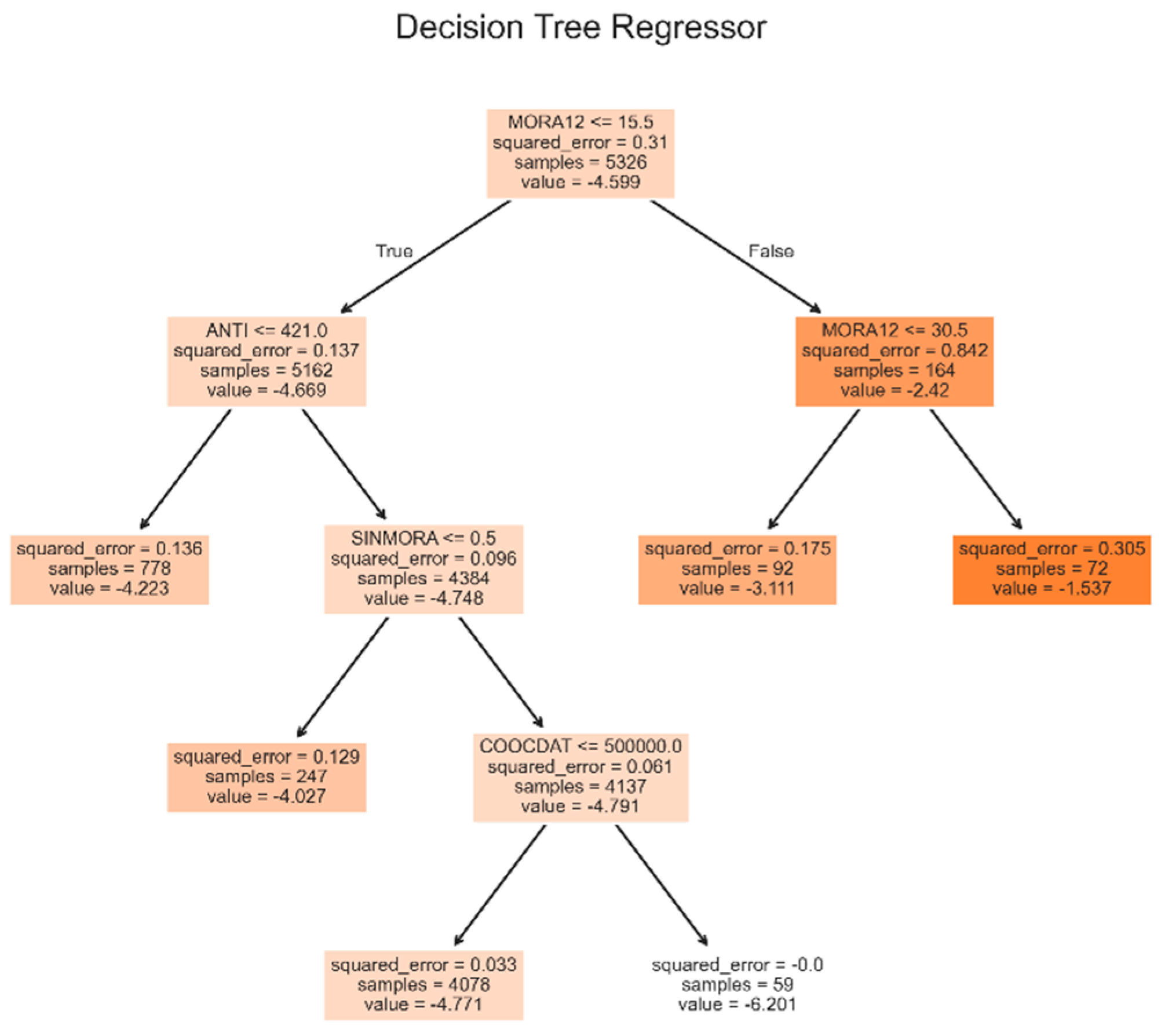
The most important feature of this model was MORA12, with a score of 0.674, followed by ANTI (score = 0.136) and SINMORA (score = 0.101). Finally, the COOCDAT score was 0.089, and the AP score was 0. The residuals of this model had a mean of 1.06 × 10⁻² and a standard deviation of 0.248.
Random forest models were also evaluated, with the best performer having 226 estimators and a ccp_alpha of 1.02 × 10⁻². With this model, the validation RMSE was 0.237, the test RMSE was 0.240, and the test R2 was 0.825. The most important feature of this model was MORA12, with a score of 0.673, followed by ANTI (score = 0.140) and SINMORA (score = 0.097). Finally, the COOCDAT score was 0.090, and the AP score was 0. The residuals of this model had a mean of 7.99 × 10⁻³ and a standard deviation of 0.24.
XGBoost models were also evaluated. Of these, the one with which the best results were obtained had the following hyperparameters: colsample_bytree: 0.755, gamma: 0.170, learning_rate: 0.156, max_delta_step: 2, max_depth: 4, min_child_weight: 8, n_estimators: 422, reg_alpha: 1.009 × 10⁻², reg_lambda: 4.787, subsample: 0.624. With this model, the validation RMSE was 0.216, the test RMSE was 0.226, and the test R2 was 0.845. In this model, the average of the residuals was 3.23 × 10⁻³, and the standard deviation was 0.227. The most important feature of this model was SINMORA, with a score of 0.593, followed by MORA12 (score = 0.170) and COOCDAT (score = 0.166). Lastly, the ANTI feature had a score of 0.054 and AP 0.018.
The last family of models evaluated was the LightGBM. Of these, the one that gave the best results had the following hyperparameters: colsample_bytree: 0.648, learning_rate: 0.071, max_depth: 13, min_child_samples: 30, n_estimators: 134, num_leaves: 74, reg_alpha: 1.592, reg_lambda: 0.277, subsample: 0.518. With this model, the validation RMSE was 0.216, the test RMSE was 0.221, and the test R2 was 0.852. In this model, the residuals had a mean of 4.27 × 10⁻³ and a standard deviation of 0.222. The most important variable in this model was MORA12 (normalized score = 0.541), followed by SINMORA (normalized score = 0.191) and ANTI (normalized score = 0.133). Finally, the COOCDAT score was 0.093, and the AP score was 0.043.
Table 1 summarizes the results of the metrics obtained with each model evaluated. It is observed that the model yielding the best results is LightGBM, although the other ensemble models evaluated (Random Forests and XGBoost) also provided satisfactory results.
Figure 4 shows the relative importance of the features in each assembly model evaluated. It is found that for 3 of these models, the most important feature is MORA12, and only for the XGBoost model is SINMORA. What all models do not agree on is that the AP feature is the least important, to the point that for decision tree models and random forests, it has no importance.
Although they are not directly comparable with the sizes of the coefficients of each feature in the linear Ridge model, it is interesting to note that in this model, the highest coefficient, in absolute value, corresponds to the SINMORA feature (0.800), followed by MORA12 (0.178) and COOCDAT (0.154), coinciding with the order of importance of the XGBoost model.
4.3.3. SHAP Global Analysis of the LightGBM Model
Given that the LightGBM model yielded the best results and that it is essential for the entity to understand how the model's characteristics influence its predictions, an interpretability analysis was conducted using SHAP. This analysis facilitates the justification of decisions to associates or users, thereby promoting trust and confidence among them.
First, a global interpretability analysis was conducted, the results of which are shown in Figure 5, to understand how the variables impact the predictions. Low values in the ANTI and SINMORA features result in an increased predicted value, indicating a higher risk. Additionally, high values in the MORA12 feature also increase the prediction value. Finally, high values in COOCDAT cause the prediction value to decrease; that is, subjects with high values in this feature tend to have a better risk rating.
A similar analysis, conducted only for high-risk loans (B rating or higher), reveals that, in this case, the most significant characteristics are MORA12 and SINMORA, with the other characteristics having a minor impact.
4.3.4. SHAP Local Analysis of LightGBM Model
With SHAP, local analysis can also be done, identifying how each characteristic influences a prediction. For example, Figure 6 illustrates the case of a subject with low risk. For this subject, the prediction was –4.823, which is a lower value than the base prediction, which is –4.6 (the base value corresponds to the average of the values of the target variable). It is observed that the lowest prediction is due to the values of the characteristics ANTI (2185, a high value), SINMORA (1, a high value), and MORA12 (0, a low value). On the other hand, the value of COOCDAT (0, a low value) causes the value of the prediction to rise; that is, it goes in the opposite direction of the final prediction.
Notably, the impact of each feature is not necessarily consistent with the relative importance of the features identified in the global analyses. Thus, in this case, it is observed that the ANTI feature has the most significant impact on prediction, while in global analyses, it is only the third most important.
4.4. Models for Non-Debit Consumer Credit
For debit consumer credit, several regression models, both linear and based on decision trees, were evaluated. For non-debit consumer credit, the best results obtained are presented below.
4.4.1. Linear Regression Model
The linear model that yielded the best results was a Ridge model with λ = 0.164, a power transformation of the numerical variables, and the elimination of outliers (observations above the 99th percentile) for the AP and SALPRES variables. With this model, a validation RMSE of 1.30, a test RMSE of 1.34, and an R2 of 0.768 were obtained.
The equation resulting from this model was:
Z = -0.733 + 2.104 x MORA12 + 0.098 x SALPRES – 0.245 x ANTI – 0.380 x AP - 1.421*ACTIVO
The residuals of this model had a mean of 3.01× 10⁻² and a standard deviation of 1.344.
4.4.2. Tree-Based Models
With a single decision tree, the best model obtained, as shown in Figure 7, had a complexity coefficient (ccp_alpha) of 2.21 × 10⁻². With this model, the validation RMSE was 0.486, the test RMSE was 0.476, and the test R-squared value was 0.971. It is worth clarifying that this model nor the following ones underwent any preprocessing of variables.
The most important variable in this model is MORA12, with a score of 0.974, followed by ANTI (score = 0.015) and AP (score = 0.012). Finally, the score of SALPRES and Active was 0. The residuals of this model had a mean of -1.50 × 10⁻² and a standard deviation of 0.476.
With random forest models, the one that gave the best results had 316 estimators and a ccp_alpha of 2.96e-4. With this model, the validation RMSE was 0.296, the test RMSE was 0.280, and the test RMSE was 0.990. In this model, the mean of the residuals was -5.24 × 10⁻⁴, and the standard deviation was 0.280. The most important feature of this model was MORA12, with a score of 0.955, followed by ANTI (score = 0.021) and Active (score = 0.009). Finally, the AP feature had a score of 0.008, and SALPRES had a score of 0.007.
With XGBoost models, the one that gave the best results had these hyperparameters: colsample_bytree: 0.982, gamma: 1.555, learning_rate: 0.152, max_delta_step: 4, max_depth: 9, min_child_weight: 8, n_estimators: 266, reg_alpha: 1.986× 10⁻³, reg_lambda: 2.616, subsample: 0.987. With this model, the validation RMSE was 0.332, the test RMSE was 0.294, and the test R2 was 0.989. In this model, the mean residuals were 6.80 × 10⁻⁵, and the standard deviation was 0.295. The most important feature of this model was MORA12, with a score of 0.918, followed by Active (score = 0.034) and AP (score = 0.021). Finally, the AP feature had a score of 0.021, and SALPRES had a score of 0.006.
The last model evaluated, and the one that gave the best results was a LightGBM regression model. With this model, the validation RMSE was 0.288, the test RMSE was 0.276, and the test R2 was 0.990. In this model, the mean residuals were 1.75 × 10⁻³, and the standard deviation was 0.272. The values of the hyperparameters tuned in this model were: colsample_bytree: 0.963, learning_rate: 0.245, max_depth: 11, min_child_samples: 16, n_estimators: 168, num_leaves: 47, reg_alpha: 6.660, reg_lambda: 0.938, subsample: 0.818. The most important feature of this model was MORA12, with a normalized score of 0.966, followed by ANTI (score = 0.017) and AP (score = 0.014). Lastly, the SALPRES feature had a score of 0.003, and Active had a score of 0.000.
Table 4 summarizes the results of the metrics obtained with each model evaluated. It is observed that the model yielding the best results is LightGBM, although the other ensemble models evaluated (Random Forests and XGBoost) also provided satisfactory results.
Figure 8 shows the relative importance of the features in each assembly model evaluated. It is found that in all these models, the most important feature is MORA12. It is also noted that, in general, all other features have little importance in the models.
Although they are not directly comparable with the sizes of the coefficients of each feature in the linear Ridge model, it is interesting to note that in this model, the highest coefficient, in absolute value, corresponds to the MORA12 feature (2.104), followed by Activo (1.421) and AP (0.380), coinciding (again) with the order of importance of the XGBoost model.
4.4.3. Global SHAP Analysis of LightGBM Model
Regarding the debit consumer portfolio, an interpretability analysis was conducted using SHAP. The global analysis (see Figure 9) shows that low values of MORA12 have a negative impact on the value of Z, and high values have a positive impact. Low values of ANTI and AP also have a positive impact, although not as significant as MORA12. However, low SALPRES values negatively impact the Z value.
On the other hand, for subjects with an elevated level of risk, it is observed that the most important characteristic remains MORA12. However, ANTI and AP exchange their positions, although the direction of the impacts remains the same as in the general case.
4.4.4. SHAP Local Analysis of LightGBM Model
Figure 10 corresponds to a SHAP waterfall plot visualization, which enables the decomposition and analysis of the prediction generated by the model for a particular individual, allowing for the accurate interpretation of the contribution of each explanatory feature to the model's result.
For example, we will present a local analysis conducted on a high-risk individual. The model has a base prediction expectation of –2.073. From this reference point, the marginal contributions of each customer feature are identified, which modify this prediction until a final value of 2.031 is reached. The feature with the most significant impact is MORA12 (whose value is 270 days (about 9 months) of default), which generates a positive contribution of +3.94 units to the prediction, evidencing a strong association between high levels of default in the last 12 months and the increase in the credit risk rating assigned by the model. This feature dominates the explanation of the result, suggesting that the history of recent defaults is the primary determinant of the risk profile in this case. Other features have marginal impacts: ANTI (permanence in the institution of 1360 days) increases the prediction by +0.22.
On the other hand, the AP feature (with a value of $216,274 in available contributions) has a mitigating effect, with a contribution of –0.12, a financial feature that reduces the perceived risk. Finally, SALPRES (Ratio of balance to loan value 0.778) provides a small positive contribution (+0.05) without significantly affecting the model's decision. The weighted sum of these effects enables the model to adjust its prediction from the average value to an individualized output, which, in this case, represents an adverse credit rating.
5. Discussion
Recent regulatory reforms in Colombia's solidarity sector reflect a global trend of alignment with the Basel II and III agreements. In particular, there is a significant transition between the reference model used in 2024 and the new model adopted in 2025 for credit risk assessment. The 2024 model, described in Section 3, using equations (1) and (2), incorporates multiple binary variables that represent the structural characteristics of the associate. On the other hand, the 2025 model, as seen in equations (5) and (6), focuses more clearly on variables related to credit behavior, especially those associated with non-performing loans.
Debit consumer credit 2025
Z = -1.523 -2.081×EA+2.495 × MORA1230 +3.062 × MORA1260 – 0.575 × SINMORA +0.319×MORA2430N+1.615 ×MORA3660
Non-Debit consumer credit 2025
Z = -1.523 -2.081×EA+2.495 × MORA1230 +3.062 × MORA1260 – 0.575 × SINMORA +0.319×MORA2430N+1.615 ×MORA3660
These models prioritize variables directly associated with the history of default, dropping some features. This simplification reflects a view more focused on the real payment behavior of the associate, which is consistent with the principles of the Basel II internal rating approach (IRB), which promotes models based on observed credit experience. In this context, the proposed model based on Ridge regression and continuous variables fits naturally and precisely into the new regulatory framework. Unlike traditional regulatory models, which transform variables into discrete indicators (e.g., presence or absence of default in ranges of days), the Ridge model preserves the richness of the original information by using continuous variables and aligns with the logic of regulatory changes implemented in 2025.
On the other hand, the advantage in terms of predictive accuracy of the LightGBM model is evident in the results obtained. For the debit consumer portfolio, LightGBM achieved an RMSE of 0.224 and an R² of 0.847; for the non-debit portfolio, it obtained an RMSE of 0.272 and an R² of 0.990. These values reflect a much higher fit than linear models or simple trees with the same variables. In other words, LightGBM captures much of the variability of loss that regulatory and traditional models leave unexplained. This finding is consistent with previous studies showing that tree-boosting methods (such as LightGBM or XGBoost) tend to outperform classical regression techniques in predictive performance. Additionally, the use of LightGBM provides flexibility in the face of future regulatory changes and facilitates internal auditing.
As a data-trained model, it can be periodically retrained with new information or easily incorporate additional indicators without waiting for regulatory reform. Although tree-based models are often considered complex ("black boxes"), this limitation was mitigated using the SHAP interpretability technique, which generates clear numerical explanations for each credit decision. In practice, this enables auditors and regulators to understand the factors that contributed to a low score or adverse rating while complying with the transparency requirements of financial supervision.
Given the above, the SES Reference Model offers a uniform and transparent scheme (collective approach with an A–E rating) that serves as a mandatory baseline. However, entities can leverage advanced techniques that are internally aligned with the Basel II Advanced Internal Ratings-Based (IRB) approach. An accurate internal model not only strengthens the management of one's own risk but also optimizes the use of capital: by better estimating the expected loss, the excess capital required by conservative standards is reduced. In this way, LightGBM does not contradict the regulation but rather complements it: it adheres to the basic guidelines of the Solidarity Superintendence while extracting additional value from the data to improve credit rating and domestic capital adequacy.
6. Conclusions
The LightGBM model demonstrates a superior ability to capture the complexity of credit behavior in solidarity sector cooperatives. In comparison, regulatory linear models. Ridge performs poorly on LightGBM, in part because it is unable to model nonlinear relationships between variables. One of the main strengths of this approach is the use of continuous financial variables, which enable the detection of subtle differences between partners. However, a key point to highlight in terms of practical applicability is the incorporation of SHAP analysis, which facilitates the interpretation of the risk scores generated by LightGBM. SHAP enables cooperatives to identify the variables that have the most significant impact on the risk of default based on real-time data and to communicate this information clearly to members, managers, control entities, and supervisors. This feature makes LightGBM not only a highly accurate model but also a tool aligned with the principles of governance, traceability, and accountability required in modern risk management systems.
This research opens multiple lines. Among these are the incorporation of alternative data (such as transactional information or digital behaviors), the use of deep learning models combined with interpretability based on SHAP, and the multicenter validation of the model using data from different cooperatives across the country. The development of complementary models that estimate the expected loss, integrating the dimensions of exposure to non-compliance and the severity of the loss, as well as the probability of non-compliance at the associate or segment level, based on the scores obtained by the current models.
Author Contributions
Conceptualization, M.A and L.M; methodology, M.A.; software, J.Q, A.O, L.U.; validation, J.Q, A.O, L.U ; formal analysis, M.A, L.M, J.Q, A.O, L.U investigation, M.A, L.M, J.Q, A.O, L.U.; resources, M.A, L.M, J.Q, A.O, L.U.; data curation, M.A, J.Q, L.U ,writing—original draft preparation, M.A, L.M, J.Q, A.O, L.U.; writing—review and editing, M.A, L.M, J.Q, A.O, L.U.; visualization, M.A, L.M, J.Q, A.O, L.U supervision, M.A.; project administration, M.A.; funding acquisition, M.A, L.M, J.Q, A.O, L.U. All authors have read and agreed to the published version of the manuscript.
Funding
This research received no external funding.
Informed Consent Statement
Not applicable.
Data Availability Statement
The data supporting the findings of this study are available from the corresponding author upon reasonable request.
Conflicts of Interest
The authors declare no conflicts of interest.
Appendix A. Definition of Variables

Table A1.
Variables Indicating the Member’s Relationship and Solvency.
| Variable | Regulatory Model Definition | Proposed Model |
|---|---|---|
| EA |
Corresponds to the member’s status in the evaluation month; it takes the value 1 if the member is “active”, otherwise it takes the value zero. | Corresponds to the member’s status in the evaluation month; it takes the value 1 if the member is “active”, otherwise it takes the value zero. |
| AP |
The debtor has contributions in the solidarity organization; it takes the value 1 if the amount of contributions is greater than zero, otherwise it takes the value zero. | Total contribution balance in the evaluation month |
| REEST |
It takes the value 1 if the loan is restructured, otherwise the value is zero. | Takes the value 2 or 4. |
| CUENAHO |
If the debtor has a “Savings Account” product with a balance >1 and active status in the solidarity organization, it takes the value 1, otherwise it takes the value zero. | Savings Account balance in the evaluation month |
| CDAT | If the debtor has an active “CDAT” product in the solidarity organization, it takes the value 1, otherwise it takes the value zero. | CDT balance in the evaluation month |
| COOCDAT |
If the organization type is “Savings and Credit Cooperative” and the member has an active CDAT with the Cooperative, it takes the value 1, otherwise the value is zero. | CDT balance in the evaluation month |
| PER |
If the debtor has “Permanent Savings” in the solidarity organization, it takes the value 1, otherwise it takes the value zero. | Permanent Savings balance in the evaluation month |
| SALPRES |
If the balance/loan ratio is less than 20% it takes the value 1, otherwise the value is zero. | Total balance/loan |
| TC |
Type of loan installment; it takes the value 1 if the installment is not fixed, otherwise it takes the value zero. | Not considered in the model since it is a constant |
Table A2.
Seniority Variables.
| Variable | Regulatory Model Definition | Proposed Model |
|---|---|---|
| ANTIPRE1 | Corresponds to the length of time the member has been affiliated with the organization at the date the loan was requested; if it is less than or equal to one month, it takes the value 1, otherwise it takes the value zero. | Corresponds to the length of time the member has been affiliated with the organization. |
| ANTIPRE2 | Corresponds to the length of time the member has been affiliated with the organization at the date the loan was requested; if it is more than 36 months, it takes the value 1, otherwise it takes the value zero. | Corresponds to the length of time the member has been affiliated with the organization. |
| VIN2 | Corresponds to the length of time the member has been affiliated with the solidarity organization; if it is more than 120 months, it takes the value 1, otherwise it takes the value zero. | Corresponds to the length of time the member has been affiliated with the organization. |
Table A3.
Variables maximum arrears.
| Variable | Regulatory Model Definition | Proposed Model |
|---|---|---|
| MORA1230 | If the maximum arrears in the last 12 months are between 31 and 60 days, it takes the value 1; otherwise, the value is zero. | Corresponds to the maximum arrears in the last 12 months. |
| MORA1260 | If the maximum arrears in the last 12 months are greater than 60 days, it takes the value 1; otherwise, the value is zero. | Corresponds to the maximum arrears in the last 12 months. |
| MORA15 | If the maximum arrears in the last 12 months are between 16 and 30 days, it takes the value 1; otherwise, it takes the value zero. | Corresponds to the maximum arrears in the last 12 months. |
| MORA2430 | If the maximum arrears in the last 24 months are between 31 and 60 days, it takes the value 1; otherwise, the value is zero. | Corresponds to the maximum arrears in the last 24 months. |
| MORA2460 | If the maximum arrears in the last 24 months are greater than 60 days, it takes the value 1; otherwise, the value is zero. | Corresponds to the maximum arrears in the last 24 months. |
| MORA2430N | If the maximum arrears in the last 24 months are between 31 and 60 days and MORA1230 is equal to 0, it takes the value 1; otherwise, the value is zero. | Corresponds to the maximum arrears in the last 24 months. |
| MORA3615 | If the maximum arrears in the last 36 months are between 1 and 15 days, it takes the value 1; otherwise, the value is zero. | Corresponds to the maximum arrears in the last 36 months. |
| MORA3660 | If the maximum arrears in the last 36 months are between 31 and 60 days, it takes the value 1; otherwise, the value is zero. | Corresponds to the maximum arrears in the last 36 months. |
| SINMORA | If the debtor did not present any arrears in the last 36 months, it takes the value 1; otherwise, the value is zero. | Takes the value 1 if the variable Max-arrears-36 is equal to zero; otherwise, it takes the value zero. |
| MORA315 | If the maximum arrears in the last 3 months are between 16 and 30 days, it takes the value 1; otherwise, the value is zero. | Corresponds to the maximum arrears in the last 3 months. |
| MORTRIM | Takes the value 1 if the debtor presented one or more delinquencies of between 31 and 60 days in the last 3 months; otherwise, it takes the value zero. | Corresponds to the maximum arrears in the last 3 months. |
References
- Aguilar-Valenzuela, G. R.; Vilca, E. M. Algoritmos para Machine Learning utilizados en la Gestión de Riesgo Crediticio en Perú: Machine Learning Algorithms used in Credit Risk Management in Peru. Micaela Revista de Investigación-UNAMBA 2024, 5(1), 30–35. [Google Scholar] [CrossRef]
- Bischl, B.; Binder, M.; Lang, M.; Pielok, T.; Richter, J.; Coors, S.; Boulesteix, A.-L. Hyperparameter Optimization: Foundations, Algorithms, Best Practices and Open Challenges. Reseñas interdisciplinarias de Wiley 2021. [Google Scholar] [CrossRef]
- Bussmann, N.; Giudici, P.; Marinelli, D.; Papenbrock, J. Explainable Machine Learning in Credit Risk Management. Computational Economics 2021, 57(1), 203–216. [Google Scholar] [CrossRef]
- Castro, J. Aplicación de machine learning en la gestión de riesgo de crédito financiero: Una revisión sistemática. Interfases 2022, 160–178. [Google Scholar] [CrossRef]
- Chen, T.; Guestrin, C. XGBoost: A Scalable Tree Boosting System. In Proceedings of the 22nd ACM SIGKDD International Conference on Knowledge Discovery and Data Mining; 2016; pp. 785–794. [Google Scholar]
- Comité de Supervisión Bancaria de Basilea. Basilea III: Marco regulatorio global para reforzar los bancos y los sistemas bancarios (versión revisada). Obtenido de Banco de Pagos Internacionales. 2011. Available online: https://www.bis.org.
- Donovan, J.; Jennings, J.; Koharki, K.; Lee, J. Measuring credit risk using qualitative disclosure. Review of Accounting Studies 2021, 815–863. [Google Scholar] [CrossRef]
- Freire, Z. G. Clasificación de riesgo crediticio mediante técnicas de Machine Learning para una institución financiera. ESPOL. FCNM. 2024. [Google Scholar]
- Friedman, J. H.; Robert, T.; Trevor, H. Elements of Statistical Learning; Universidad de Pennsylvania: Pennsylvania, 2009. [Google Scholar]
- Gambacorta, L.; Huang, Y.; Qiu, H.; Wang, J. How do machine learning and non-traditional data affect credit scoring? New evidence from a Chinese fintech firm. Journal of Financial Stability 2024, 73–101. [Google Scholar] [CrossRef]
- Gatla, T. R. Machine learning in credit risk assessment: analyzing how machine learning models are transforming the assessment of credit risk for loans and credit cards. Journal of Emerging Technologies and Innovative Research 2023, 10, k746–k750. [Google Scholar]
- Geurts, P.; D., E.; Wehenkel, L. Extremely randomized trees. Machine Learning 2006, 3–42. [Google Scholar] [CrossRef]
- Gonzalez, P. M.; Coveñas de León, M. Algoritmos para Machine Learning utilizados en la Gestión de Riesgo Crediticio en Perú: Machine Learning Algorithms used in Credit Risk Management in Peru. Micaela Revista de Investigación-UNAMBA s.f., 30–35. [Google Scholar]
- Grau, Á. J. Machine Learning y riesgo de crédito. Universidad pontificia comilla 2020. [Google Scholar]
- Jackson, P. Regulatory implications of credit risk modelling. Journal of Banking & Finance 24 2020, 1–14. [Google Scholar] [CrossRef]
- Jorion, P. Valor En Riesgo: El nuevo paradigma para el control de riesgos con derivados. Limusa. Obtenido de. 2000. Available online: https://books.google.com.co/books?id=bcnaPQAACAAJ.
- Libda, R. The Impact of Fintech on Credit Risk Management: An Applied Study on the Egyptian Banking Sector. Journal of Alexandria University for Administrative Sciences 2024, 61(5), 391–422. [Google Scholar] [CrossRef]
- Lundberg, S. M.; Lee, S. I. A unified approach to interpreting model predictions. Advances in neural information processing systems 2017, 1–11. [Google Scholar]
- Machado, M.; Karray, S. Assessing credit risk of commercial customers using hybrid machine learning algorithms. Expert Systems with Applications 2022. [Google Scholar] [CrossRef]
- McDonald, G. Ridge regression. In Wiley Interdisciplinary Reviews: Com-putational Statistics; 2009; pp. 93–100. [Google Scholar]
- Meng, K.; Finley, T.; Wang, T.; Chen, W.; Ma, W.; Liu, T. Y. Lightgbm: A highly efficient gradient boosting decision tree. Advances in neural information pro-cessing systems 2017, 30. [Google Scholar]
- Superintendencia de la Economia Solidaria. Sistema de Administración del Riesgo de Crédito, SARC. Sistema de Administración del Riesgo de Crédito, SARC, 2024. [Google Scholar]
- Valenzuela, A.; R, V. Algoritmos para Machine Learning utilizados en la Gestión de Riesgo Crediticio en Perú: Machine Learning Algorithms used in Credit Risk Management in Peru. Micaela Revista de Investigación-UNAMBA 2024, 5–30. [Google Scholar]
- Vasquez, C. D. Análisis comparativo de algoritmos de machine learning para predecir morosidad en clientes afiliados a la entidad financiera San Francisco de Mocupe. Universidad señor de Sipan 2025, 1–13. [Google Scholar]
- Yeo, I. K.; Johnson, R. A.; Deng, X. An empirical characteristic function approach to selecting a transformation to normality. Communications for Statistical Applications and Methods 2014, 213–224. [Google Scholar] [CrossRef]
- Yeo, I.; Johnson, R. A new family of power transformations to improve normality or symmetry. Biometrik 2000, 954–959. [Google Scholar] [CrossRef]
- Yusheng, L. A Hybrid Credit Risk Evaluation Model Based on Three-Way Decisions and Stacking Ensemble Approach. Computational Economics 2024, 1–24. [Google Scholar] [CrossRef]
- Zaragoza, J. Riesgo financiero en el sector minero informal: una visión práctica. Mineria y Finanzas 2018, 11–32. [Google Scholar]
Figure 1.
Project workflow.
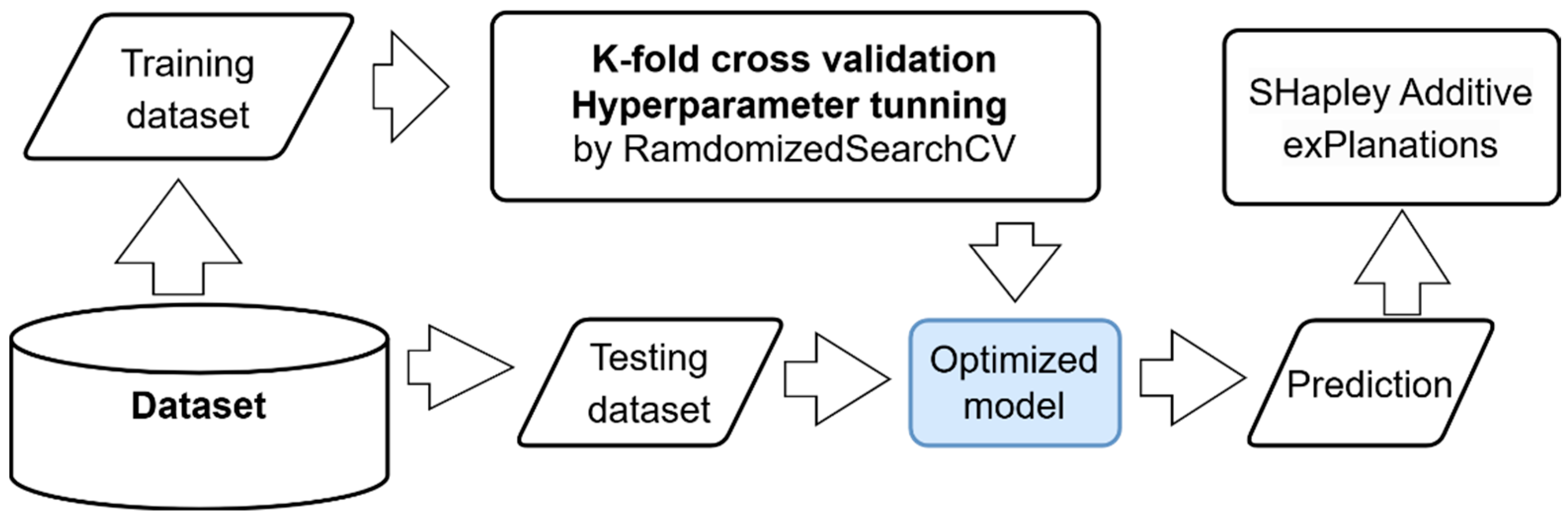
Figure 2.
A) Heatmap of Spearman correlation coefficients: B) Heatmap of Spearman correlation coefficients: debit consumer credit. non-debit consumer credit.
Figure 2.
A) Heatmap of Spearman correlation coefficients: B) Heatmap of Spearman correlation coefficients: debit consumer credit. non-debit consumer credit.
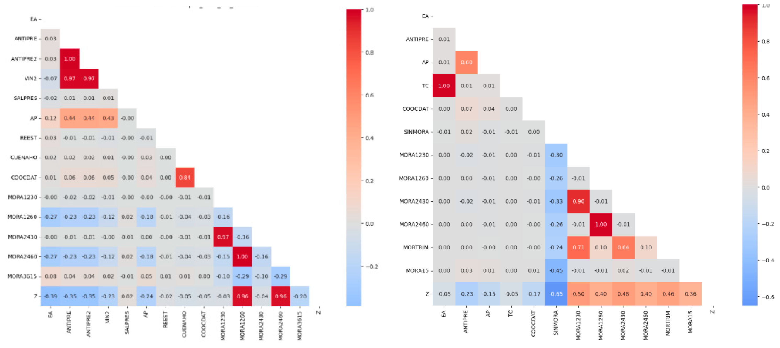
Figure 4.
Relative importance of each feature in the assembly models evaluated for the credit with debit modality.
Figure 4.
Relative importance of each feature in the assembly models evaluated for the credit with debit modality.
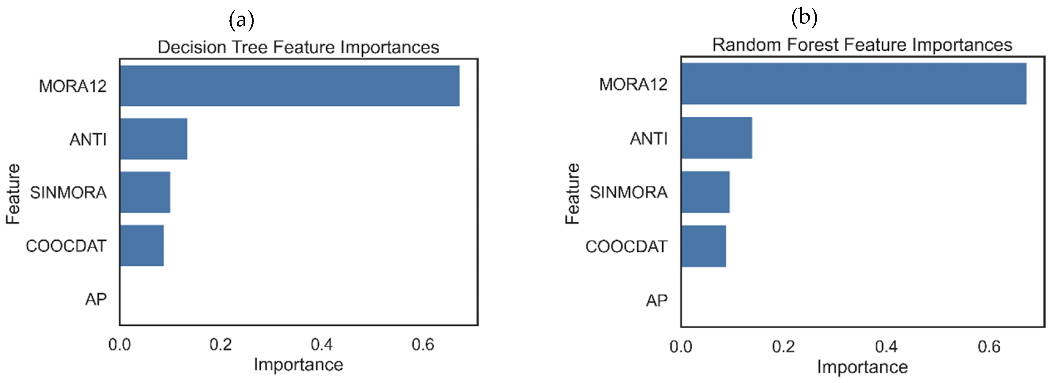
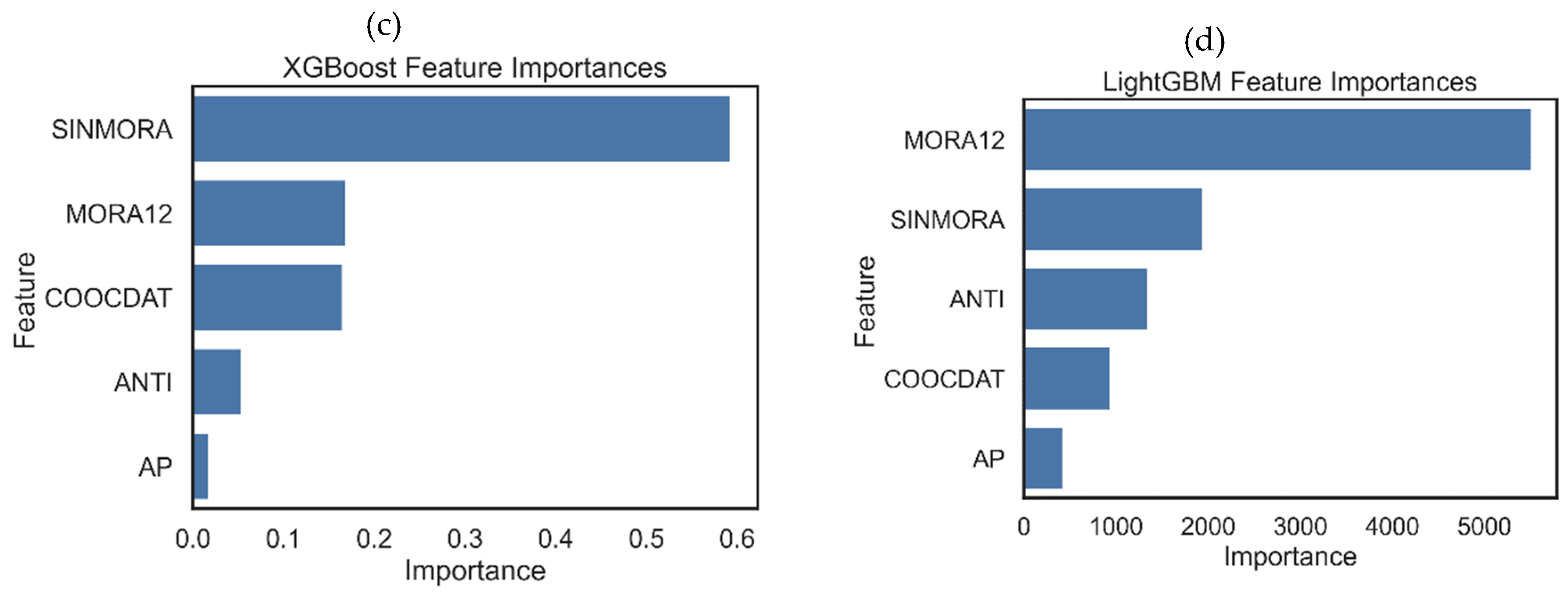
Figure 5.
Global SHAP analysis of the LightGBM model for debit consumer credit. (a) All subjects. (b) High-risk subjects (Grade B or higher).
Figure 5.
Global SHAP analysis of the LightGBM model for debit consumer credit. (a) All subjects. (b) High-risk subjects (Grade B or higher).
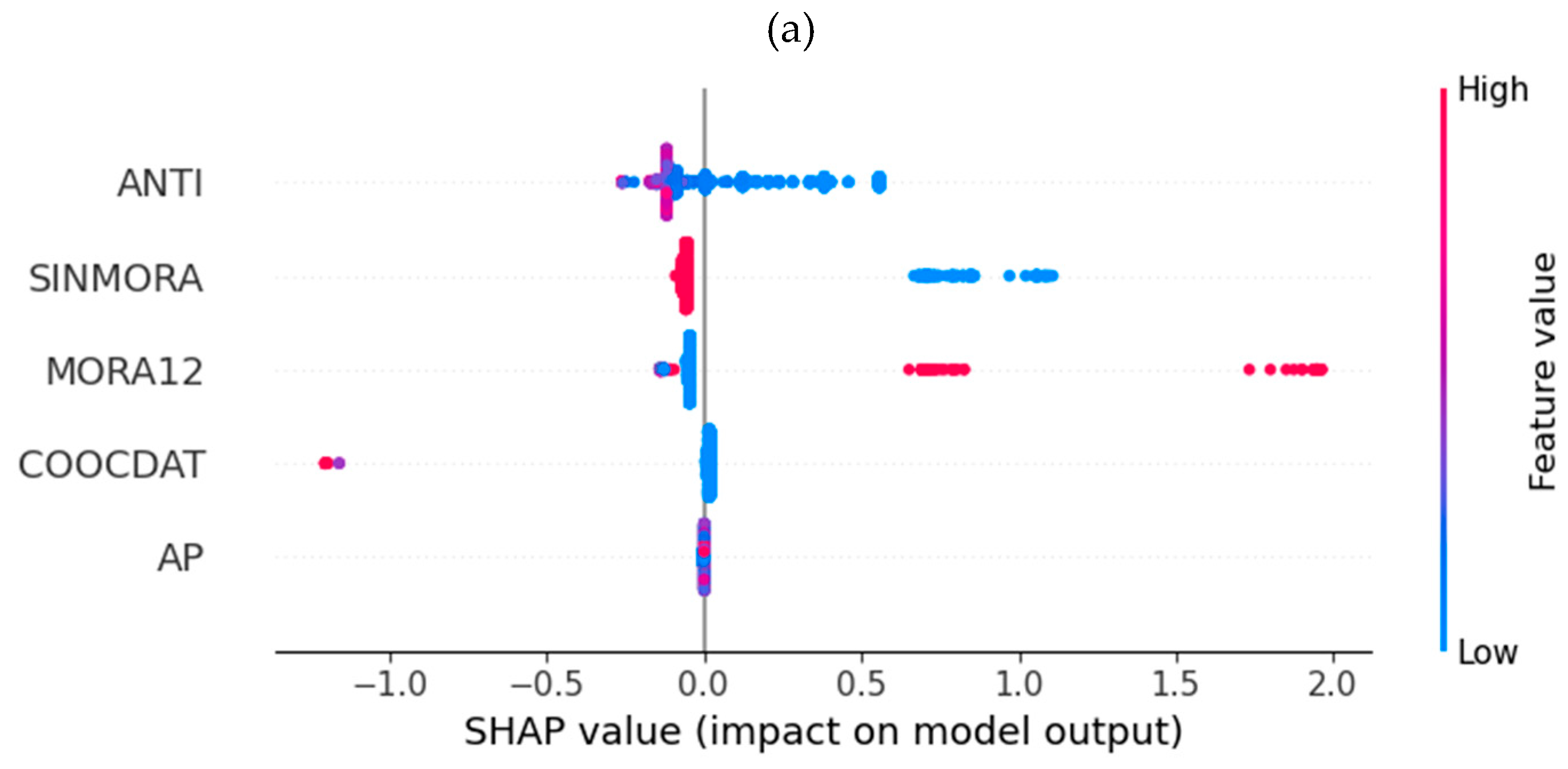
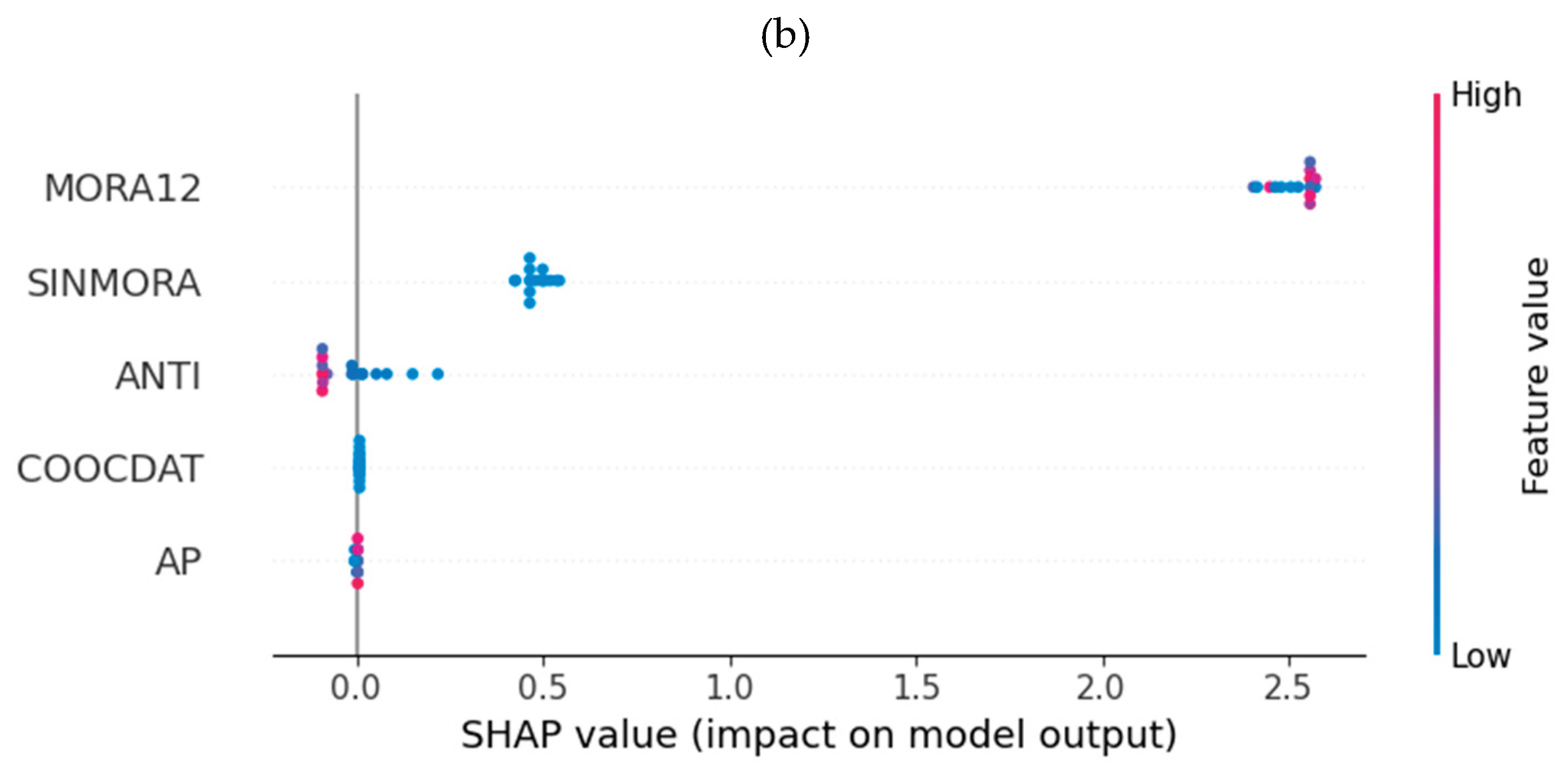
Figure 6.
SHAP local analysis of a low-risk subject in debit consumer credit.
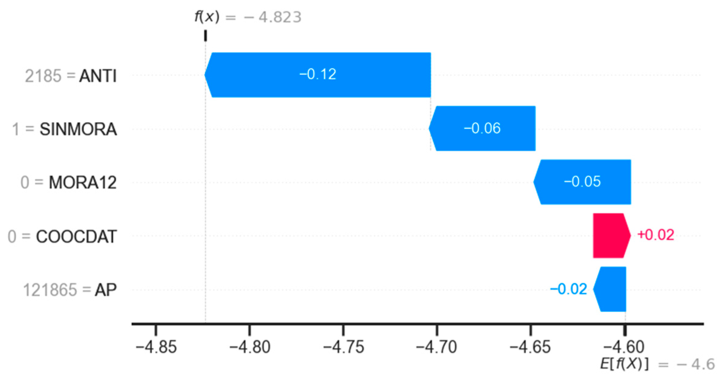
Figure 7.
Decision tree model.
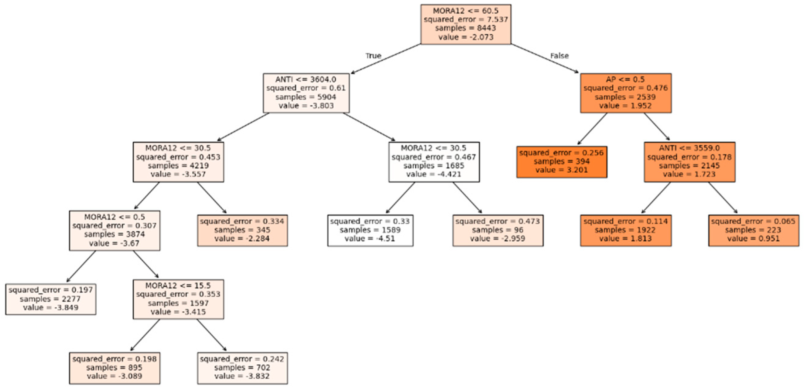
Figure 8.
Relative importance of each feature in the assembly models evaluated for non-debit credit.
Figure 8.
Relative importance of each feature in the assembly models evaluated for non-debit credit.
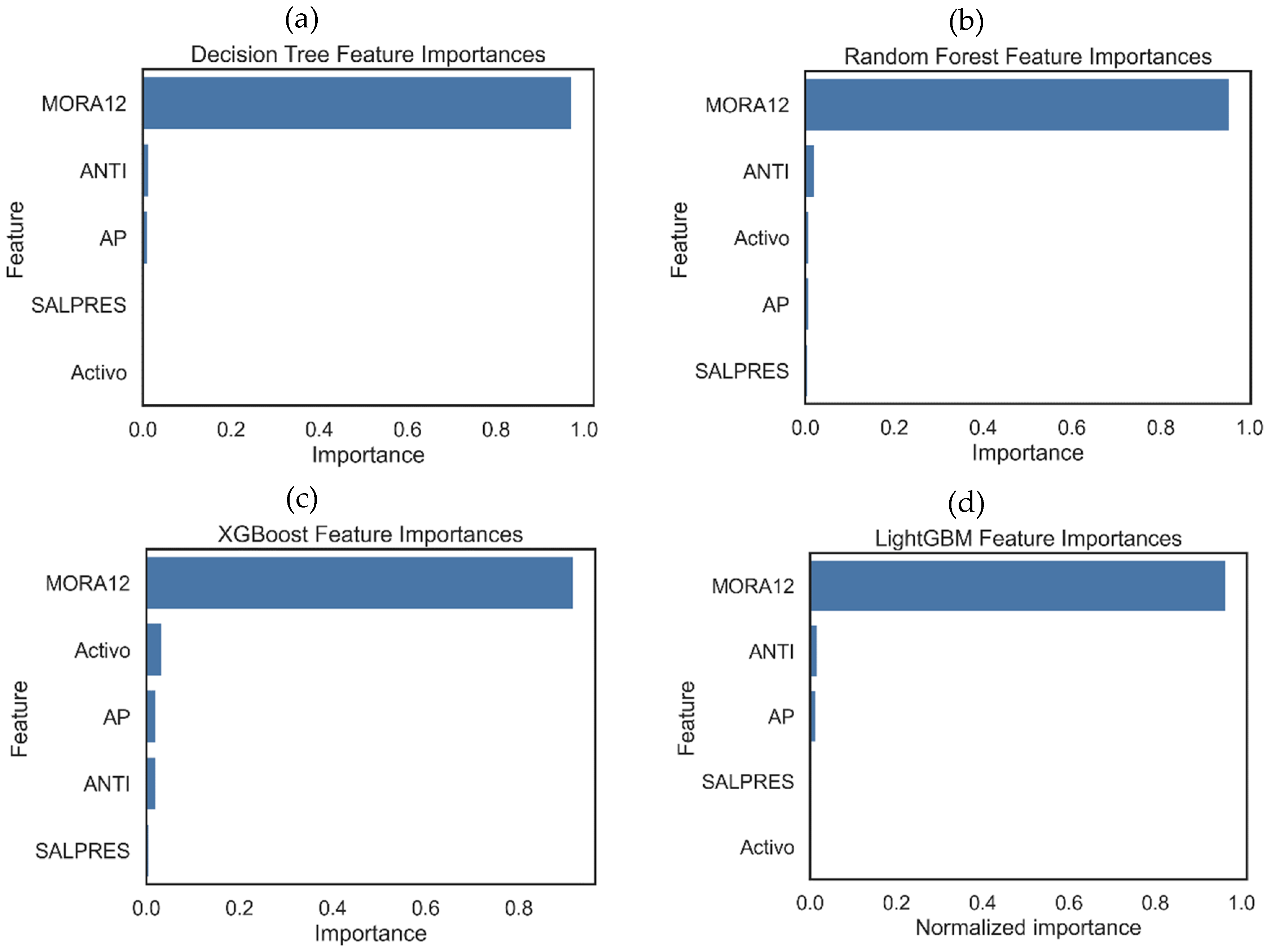
Figure 9.
Global SHAP analysis of LightGBM model for non-debit credits. (a) All subjects. (b) High-risk subjects (Grade B or higher).
Figure 9.
Global SHAP analysis of LightGBM model for non-debit credits. (a) All subjects. (b) High-risk subjects (Grade B or higher).
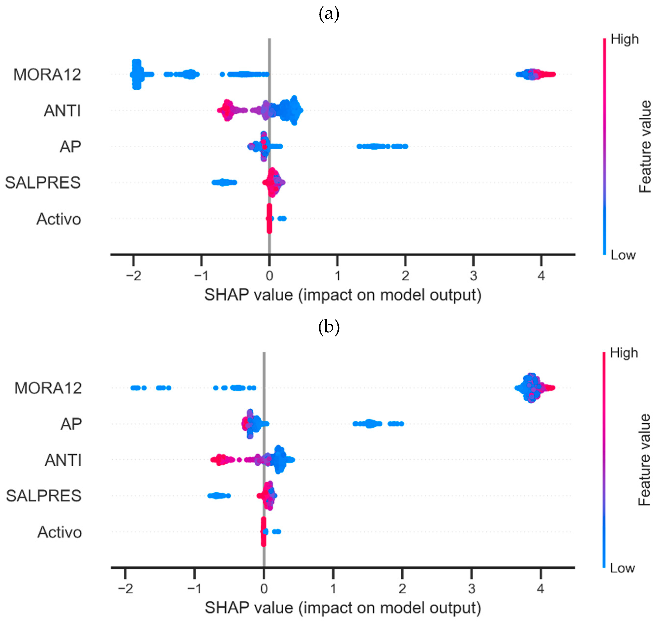
Figure 10.
SHAP local analysis of a high-risk subject in non-debit credit.
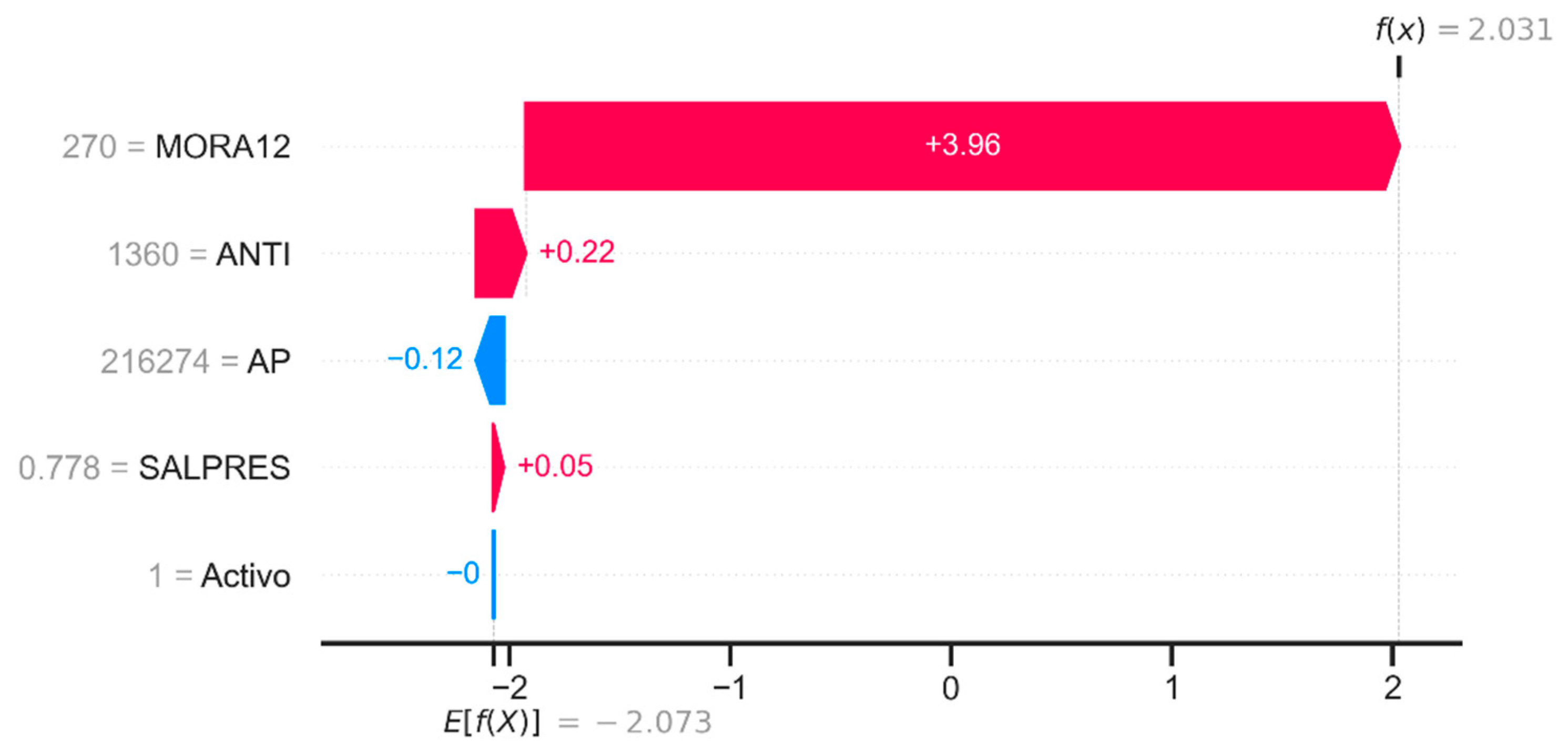
Table 1.
Metric values obtained by each of the models evaluated for debit consumer credit.
| Metric | Ridge | Decision Tree | Random Forest | XGBoost | LightGBM |
|---|---|---|---|---|---|
| Validation RMSE | 0.338 | 0.260 | 0.237 | 0.216 | 0.216 |
| Test RMSE | 0.344 | 0.248 | 0.240 | 0.226 | 0.221 |
| Test R² | 0.642 | 0.814 | 0.825 | 0.845 | 0.850 |
Table 4.
Metric values obtained by each of the models evaluated for the credits non-debit modality.
| Metric | Ridge | Decision Tree | Random Forest | XGBoost | LightGBM |
|---|---|---|---|---|---|
| Validation RMSE | 1.300 | 0.486 | 0.296 | 0.332 | 0.288 |
| Test RMSE | 1.340 | 0.476 | 0.280 | 0.294 | 0.276 |
| Test R² | 0.768 | 0.971 | 0.990 | 0.989 | 0.990 |
Disclaimer/Publisher’s Note: The statements, opinions and data contained in all publications are solely those of the individual author(s) and contributor(s) and not of MDPI and/or the editor(s). MDPI and/or the editor(s) disclaim responsibility for any injury to people or property resulting from any ideas, methods, instructions or products referred to in the content. |
© 2025 by the authors. Licensee MDPI, Basel, Switzerland. This article is an open access article distributed under the terms and conditions of the Creative Commons Attribution (CC BY) license (http://creativecommons.org/licenses/by/4.0/).
Copyright: This open access article is published under a Creative Commons CC BY 4.0 license, which permit the free download, distribution, and reuse, provided that the author and preprint are cited in any reuse.


