Submitted:
06 October 2025
Posted:
06 October 2025
You are already at the latest version
Abstract
Credit Scoring helps financial organizations to provide credit services where the advancement in computing has opened ways for credit scoring approaches with different Machine Learning (ML) techniques becoming increasingly useful. Although complex models provide better predictions, they tend to lack interpretability which is a concern for credit scoring where fairness in decision making is emphasized. This study addresses credit scoring, a vital aspect of financial risk management, by employing advanced machine learning techniques to three distinct datasets: Credit Risk Dataset (CRD), Econometric Analysis (EA), and Default of Credit Card Clients (DCC). A broad spectrum of individual classifiers, including Decision Trees, Logistic Regression, Random Forests, XGBoost, LightGBM, and CatBoost, are systematically trained and evaluated using metrics such as accuracy, F1-score, sensitivity, specificity, MCC, Cohen's Kappa, and ROC AUC. A key contribution is the Bayesian Optimized Stacking Ensemble (BO-StaEnsemble), which leverages Optuna for hyperparameter tuning of its base and meta-learners. Beyond predictive performance, we integrate statistical validation (paired t-tests, McNemar's tests) and Explainable AI (LIME, SHAP, Morris Sensitivity). Furthermore, t-SNE is utilized for visualizing model probability spaces. The BO-StaEnsemble consistently outperforms individual models across all datasets with AUC of 0.998 for CRD, 0.999 for EA, 0.974 for DCC, as well as, demonstrated consistently high agreement and classification reliability across all datasets, achieving Matthews Correlation Coefficient (MCC) and Cohen’s Kappa values of 0.9159 and 0.9147 on the CRD, 0.9903 and 0.9902 on the EA Datasets, respectively, demonstrating the power of ensemble learning, advanced optimization, and comprehensive interpretability for robust credit risk modeling.
Keywords:
BO-StaEnsemble
; Bayesian optimization
; LIME
; Morris sensitivity analysis
; t-SNE
1. Introduction
Credit Score denotes the creditworthiness of people, which helps financial organizations to provide credit services. Credit scoring is a set of decision models and their underlying techniques that aid credit lenders in the granting of credit [6,38]. It mainly focuses on classifying the credit applicants, whether they are creditworthy or non-creditworthy, based on financial data. Enhancing the performance of the credit scoring models may result in enabling credit access to an increased number of creditworthy people while reducing credit defaults. Increased financial credit access, especially from formal financial institutions, can bolster financial inclusion efforts. Limited access to formal credit access leads people to opt for rather informal sources of credit where they are compelled to pay a considerable amount of interest, particularly in the Global South context [39].
While different statistical techniques have been employed historically for credit scoring, global IT transformation and computing advancement have significantly impacted the credit scoring practices where different Machine Learning (ML) and Deep Learning (DL) techniques are becoming increasingly useful for the context of credit scoring. The effectiveness of such models has led researchers to explore this domain in depth and breadth, resulting in numerous approaches to evolve and become popular. Different learning models with single and ensemble classifiers, along with complex neural networks, are among the common approaches in Credit Scoring literature. Literature reviews have also cautioned about the interpretability of the models where more complex models result in less explainability of the predictions, which is a must to adhere to credit scoring guidelines [40]. It implies a dilemma of better prediction and explainability as more complex models seem to provide better but less interpretable predictions [10]. Researchers have experimented with different learning approaches, along with feature engineering techniques, to assess their performance. Stefan Lessmann et al., in their studies [5], assess and update the performance of state-of-the-art classification algorithms in the context of credit scoring and employ a comprehensive approach to benchmarking, evaluating a range of state-of-the-art classification algorithms like Decision Tree (DT), Support Vector Machines (SVM), Random Forests (RF), and Neural Networks (NN). The heuristic approach and ML methods are used by S. R. Islam [1] to predict potential credit default accounts from default credit card client data. Various ML models are applied in Ahmad Abd Rabuh et al.’s study [24] to generate insights into ML models while working with imbalanced datasets. While the existing research works provide suggestions for better performing models, the balance of interpretability with performance and institutional focus while granting loans are not explored. Although there are works employing Explainable AI (XAI) techniques for making the models explainable, they do not focus on the aspects of the balance between performance and interpretability of the model intermingled with the focus of the credit lenders.
The application of machine learning and deep learning to credit scoring has made significant progress yet multiple gaps persist. Most research studies analyze individual datasets or single-domain applications which restrict the ability to generalize their findings across different credit risk contexts. The predictive advantages of ensemble methods remain underexplored because researchers have not conducted systematic studies about optimizing both base learners and meta-learners through Bayesian optimization for maximum performance. The current research practice separates explainability from statistical validation when developing models instead of integrating these components during the development process. The current approaches lack both detailed model-agnostic interpretability features and rigorous hypothesis testing capabilities. The visualization technique t-SNE remains underutilized for providing clear insights about how models differentiate between creditworthy and non-creditworthy applicants. The contributions of this work are summarized as follows:
- We introduce a novel stacking framework in which both the base classifiers (Random Forest, XGBoost, Logistic Regression) and the meta-learner are jointly hyperparameter-tuned via Optuna, yielding AUCs of 0.998 (CRD), 0.999 (EA), and 0.974 (DCC) and consistently outperforming all individual and untuned ensemble baselines.
- Unlike prior work confined to a single dataset, our BO-StaEnsemble is rigorously evaluated on three famous credit-credit scoring datasets - CRD (Credit Risk Dataset), EA (Econometric Analysis) and DCC (Default of Credit card Clients), demonstrating robustness and generalizability across varied economic and demographic contexts.
- We embed paired t-tests and McNemar’s tests directly into the evaluation pipeline to assess whether observed performance differences are statistically significant, ensuring that reported gains reflect true model improvements rather than random variation.
- By combining model-agnostic techniques—LIME for local decision explanations, SHAP for global and per-instance importance, and Morris Sensitivity Analysis for feature interaction effects—we deliver fine-grained, transparent insights into the drivers of creditworthiness decisions.
- We used t-SNE to project high-dimensional model outputs into a two-dimensional space, clearly separating default vs. non-default clusters and illustrating how the ensemble synthesizes base-learner predictions into coherent, interpretable decision boundaries.
The paper follows this structure for its remaining sections: Section 2 provides an overview of the background study and Section 3 explains the materials and methods used in the research. The analysis of results appears in Section 4 followed by a conclusion in Section 5 which summarizes the findings and discusses field impact and future research directions.
2. Related Works
2.1. Comparison of Classification Approaches for Credit Scoring
Concurrent researchers have explored and compared the performance of different classification approaches for credit scoring. Stefan Lessmann et al., in their studies [5], assessed and updated the performance of state-of-the-art classification algorithms in the context of credit scoring. Their research employs a comprehensive approach to benchmarking and evaluating a range of state-of-the-art classification algorithms like Decision Trees, SVM, Random Forests, and Neural Networks. Various ML models like KNeighborsClassifier, SVC, NuSVC, Decision Tree, Random Forest, AdaBoost, XGBoost, Linear Discriminant Analysis, Naïve Bayes was applied in Ahmad Abd Rabuh et al.’s study [24] and results show XGBoost model achieved the highest accuracy. However, the lowest log loss is a big issue for that particular model, and Naïve Bayes shows improved accuracy. Yao Zou et al.’s study [25] introduced AugBoost-ELM, named a new method, a variant of Gradient Boosting Decision Trees (GBDT) that is used to improve the performance of credit scoring, which is also more efficient compared to using a Neural Network (NN). Besides these, this study examines statistical-based methods such as linear discriminant analysis (LDA) and logistic regression, artificial intelligence (AI)-based approaches such as Artificial Neural Network (ANN), Decision Tree, SVM, KNN, Naïve Bayesian model on four different datasets.
Different review papers have also assessed the performance of different models. Hayashi, in his paper [10], reviewed papers from 2015 to 2018 on Credit Scoring to prove deep belief networks (DBNs) can achieve higher accuracy than shallower networks in multiple datasets. These papers also represent replacing ML techniques with DL techniques. Elena Ivona et al., in their paper [11], proposed a high-performance and interpretable method called penalized logistic tree regression (PLTR) in 4 real-world credit scoring datasets, which can predict credit risk more accurately rather than Logistic Regression and also defines interpretability. Anton Markov et al., in their systematic review [13], found that popular baseline models for credit scoring include Logistic Regression, SVM, classifier/regression trees (CART), and Neural networks, which are widely used for more complex techniques. In contrast, ensemble models like bagging, boosting, and stacking are considered efficient alternatives. Ensuring users’ privacy through applying the Federated Learning technique is one of the main objectives of Adil Oualid et al.’s review paper from 2018 to 2022, and they used different papers on federated learning to ensure user privacy and trained models on decentralized data for their experiments [21].
Many researchers have also worked on various approaches to achieve better performance for credit scoring. The heuristic approach and ML methods are used by S. R. Islam to predict potential credit default accounts from the default credit card client dataset [1]. Extremely Random trees performed very well in terms of accuracy, precision, recall, and f1 score in that work. S. B. COŞKUN and M. TURANLI, in their paper [7], used CatBoost, XGBoost, and LightGBM models in the Home Credit Default Risk dataset from Kaggle, where almost the same results given by the models without hyperparameter tuning and model didn’t perform well in 1’s prediction. When they used Grid Search CV for hyperparameter tuning, LightGBM and XGBoost models performed well. On the other hand, Z. Qiu, Y. Li et al. [8], in their paper, used a polynomial approach, automatic approach, and manually crafted approach in the constructed dataset, including the Home Credit Default Risk dataset with Logistic Regression (LR), Random Forest, and LightGBM models where LightGBM gives the highest AUC score of 78%. Long Short Term Memory model (LSTM) is used to predict Missed payment, Purchase Estimation, and their Missed payment LSTM model compared to four classical ML algorithms: SVM, Random Forest, MLP, and Logistic Regression to help bank management in scoring credit card clients in multiple aspects [23]. The result leads to Missed payment LSTM, a neural network for consumer credit scoring, significantly performing better than conventional methods relying on feature extraction. Clement Fung et al., in their studies [2], proposed a brokered learning abstraction called TorMentor that allows it to contribute to a globally shared model. Also, the Federated Learning technique is applied for data privacy with Client API and Curator API. The case study of 007 Fenqi in China, which combines e-commerce with microloan services, offers micro-loans and installment-based retailing exclusively for college students, as observed by Carmen Leong, Barney Tan et al. [3]. Their development strategy includes facilitating peer-to-peer lending (P2P), extending customer life cycles, and building an ecosystem that gathers comprehensive data. Pranith K. Roy and Krishnendu Shaw, in their paper [14], proposed a model for Small and Medium Enterprises (SMEs) with techniques named Analytic Hierarchy Process (AHP) and TOPSIS, which can be useful for financial institutions, as claimed by Pranith K. Roy and Krishnendu Shaw. Sujatha, R et al. [47] in their study compares the predictive performance of XGBoost, CatBoost, LightGBM, and LSTM using PCA and random forest feature engineering on a corporate credit risk dataset. Results show that tree based ensembles perform best with random forest selected features while LSTM excels with PCA derived components, offering practical guidance for financial risk forecasting. Dang et al. [49] evaluates federated averaging for credit card fraud detection on the skewed European Credit Card dataset by training local models at individual banks and aggregating updates into a shared global model without exposing raw data. Experimental results demonstrate that the federated approach effectively leverages distributed data to detect fraudulent transactions while preserving privacy.
While researchers in this domain have employed various approaches to compare the performance of different classification approaches, not many have focused on the explainability of the better performing models.
2.2. Feature Selection and Explainability
There are several works in the credit scoring literature that primarily focused on explainability of the models or feature selection techniques. For example, Petter et al. identified the main contribution of their paper is to implement the explainable AI technique named SHAP to improve the reliability of the banking sector [9]. They also showed how LightGBM outperforms the bank’s current Logistic Regression model as a more accurate credit default prediction model. Reza et al. [35] demonstrated how LDA as a feature reduction technique can be useful for reducing the burden of the model’s complexity in credit scoring predictive systems. Swati Tyagi, in her paper [12], implemented different single classifiers and ensemble classifiers with sequential neural networks and found that ensemble classifiers and neural networks outperform other models. This paper also implemented the SHAP and LIME techniques for making the model interpretable in the P2P Lending Dataset. Using correlation networks and Shapley values, the model groups AI predictions based on similar underlying explanation methods applied to Niklas Bussmann et al.’s study [22] and introduces an explainable AI model for credit risk management in P2P lending. This study used the TreeSHAP method combined with XGBoost, and the Minimal Spanning Tree (a single linkage cluster) was used to simplify and interpret the structure among Shapley values. Carlos Serrano-Cinca et al.’s study [26] involves comparing two different methods for predicting whether someone will repay a loan; the first way is using a simple model called logistic regression, and it is more likely a straightforward formula, and the other one is an advanced ML algorithms, which are like complex computer programs and result conclude that the ML algorithms were better at making predictions, besides this an XAI technique named SHAP is used to deep dive to understand the how model making decision.
Additionally, influence of different feature selection techniques in the performance of the models have also gained attention of the researchers in this domain. Jasmina Nalić, Goran Martinović et al., in their paper [29], used different feature section techniques named Classifier feature evaluation (ClassFE), Correlation feature evaluator (CorrelationFE), Gain ratio feature evaluator (GainRFE), Information gain feature evaluator (InfoGainFE) and Relief feature evaluator (RefilefFE) in real-life dataset of a microfinance institution in Bosnia and Herzegovina with 32 features, where Generalized linear model and Decision Tree hybrid model gives the highest accuracy. In the paper [30], Pantelis Z. et al. used clustering and stratified k-fold cross-validation with k=10 in a German dataset with 1000 past credit applicants on 24 features. Four wrapper approaches including, ‘‘defaultGA+KNN’’, ‘‘altGA+KNN’’, ‘‘defaultGA+NB’’ and ‘‘altGA+NB’’ are used in this paper. Shrawan, in his paper [31], used different feature selection techniques: Information-gain, Gain-Ratio and Chi-Square in ML classifiers (Naïve Bayes, Random Forest, Decision Tree and SVM) on publicly available German Dataset, and this study evaluated classifiers using FNR. They found the combination of Chi-Square & Random Forest excelled at minimizing FNR, making it suitable for imbalanced data, comprising mainly retail and business data. A feature selection technique, Bolasso (Bootstrap-Lasso), is proposed in the paper [32], which shortlisted some important features. The paper applied this feature selection technique in three publicly available datasets (Lending Club, Loan Status, and German Dataset) with different ML techniques and found that Random forest with the Bolasso technique gives the highest accuracy overall. In the paper [33], they proposed a new feature selection technique, a two-stage multi-objective method that optimizes the number of features while improving the classification performance. Dalia Atif et al. [48] compares RFE RF, RFE SVM and penalized logistic regression as feature selection methods across logistic regression, random forest and linear SVM on the German Credit dataset, evaluating error rate, stability and runtime. Results show RFE RF yields the highest accuracy, RFE SVM delivers the best stability with the fastest runtime, and one stage selection matches or outperforms two stage approaches.
After a thorough review of previous work, it has been observed that, although prior studies have rigorously benchmarked individual and ensemble classifiers, introduced novel boosting variants, and explored a range of feature selection and explainability methods, they typically remain confined to single datasets or treat interpretability and statistical validation as peripheral add ons. What is missing is a unified, multi domain framework that jointly optimizes ensemble components for peak predictive performance, embeds rigorous hypothesis testing into the evaluation pipeline, and delivers fine grained, model agnostic explanations alongside intuitive visualizations of decision boundaries. Our work fills this gap by presenting a Bayesian optimized stacking ensemble that is validated across three distinct credit risk datasets, incorporates paired t tests and McNemar’s tests to ensure that performance gains are statistically sound, and leverages LIME, SHAP, Morris sensitivity analysis, and t SNE visualizations to provide comprehensive, granular insight into how creditworthiness decisions are made.
3. Methodology
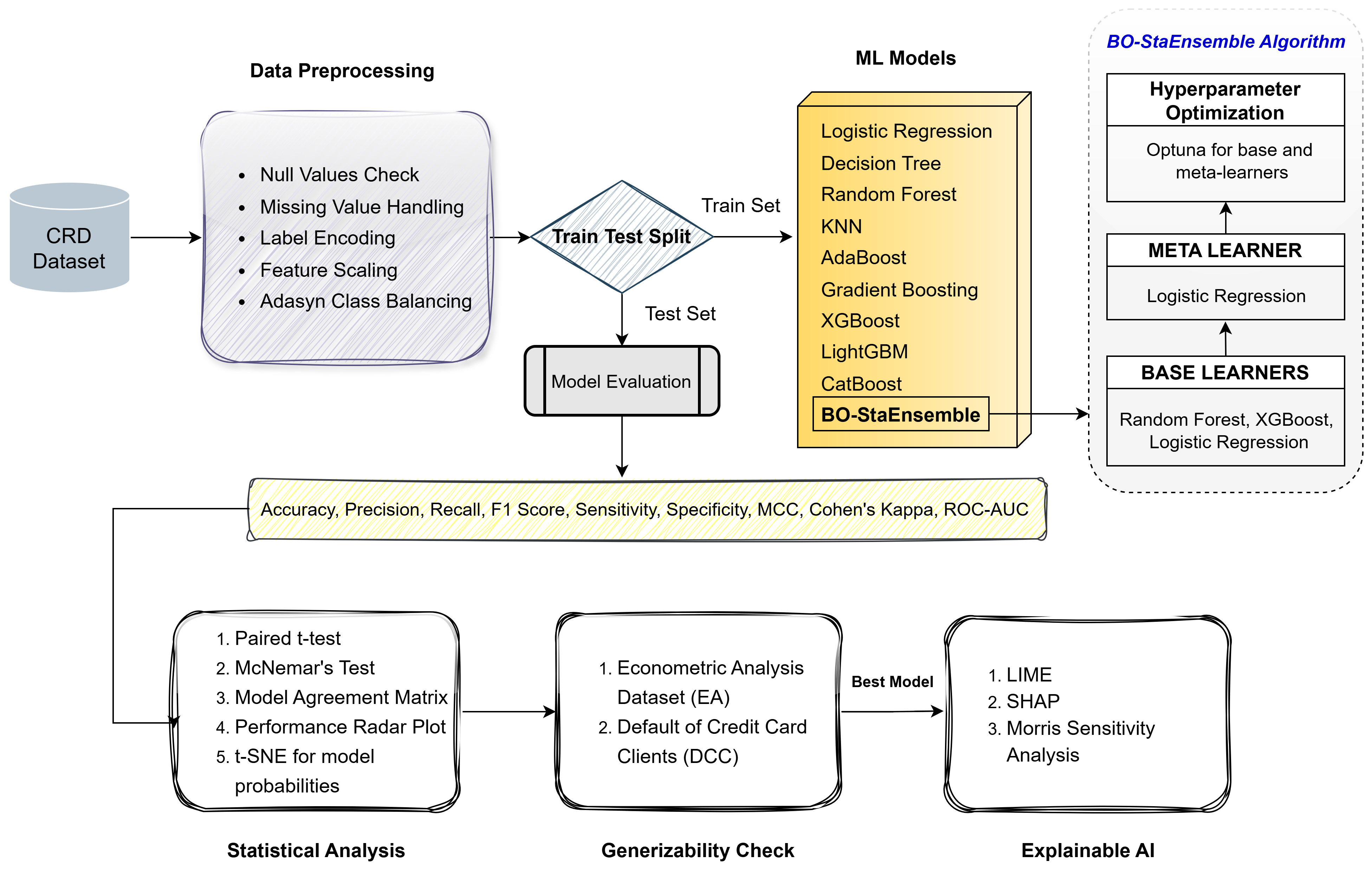
We gathered three publicly available datasets: Default of Credit Card Clients (DCC), Credit Card Data from book "Econometric Analysis” (EA), and Credit Risk Dataset (CRD). Next, we preprocessed the data to improve its cleanliness. The entire data of each dataset was then divided into two groups: the Train set (80%) and the Test set (20%). Next, we applied 10 machine learning classifiers, including our proposed BO-StaEnsemble. Five different evaluation metrics were used to evaluate the performance. Statistical Analysis with t-test, McNemar’s Test and t-SNE are used to assess the performance. Lastly, we used the Explainable AI (XAI) techniques - SHAP, Morris Sensitivity Analysis and LIME to explore the interpretability of the best performing model. The research method workflow illustrated in Figure 1, which provides the details of the research method employed in this research work.
3.1. Dataset Details
In this paper, we explored three public datasets and compared the performances of widely used ML models. Table 1 provides a description of the datasets used. All these datasets are real-world credit scoring datasets with different applications such as loans and credit cards. Although they are all credit scoring datasets, the variables they contain are different from one another. CRD contains columns simulating credit bureau data [43] having loan related features like loan intent, grade, amount, and interest, along with credit history related information like historical default and credit history length. Meanwhile, EA contains credit card data for simple econometric analysis like the number of dependents, months living at the current address, number of credit cards and accounts, and self-employment. Both CRD and EA have age, annual income, home ownership, and number of derogatory reports as common features. However, DCC, despite being a credit card dataset like EA, shares very few common features with either dataset. DCC has 23 features, most of which are regarding the payments made by the credit card clients, like the amount of bill statements, amount of previous payments, and history of past payments.
3.2. Data Preprocessing
After collecting the publicly available datasets, we applied different data preprocessing techniques. Firstly, we observed the distribution plot of target variables (shown in Figure 2). We found the datasets are quite imbalanced. Loan_status, with a value of 0, is substantially greater than 1 in the CRD dataset. However, in datasets EA and DCC, respectively, the card with "yes" and the default payment next month with a value of 0 are higher. These datasets have around one-fifth of the observations as defaults. We checked for null values and duplicate values in the dataset. EA and DCC datasets had no such values in the dataset. However, the CRD had 2 features ‘person_emp_length’ and ‘loan_int_rate,’ with 895 and 3116 entries with null values, respectively, in a total of 32581 entries. Both features are imputed with mean values. Then, we plotted histograms for all the numerical features. So, moving to the next part, we analyzed the barplot and count plot of categorical and numerical features, respectively, to observe the distribution of features. Generally, Dataset imbalance occurs due to the huge difference in the number of good borrowers and bad borrowers. So, to address this problem, we apply the ADASYN approach to the CRD, EA and DCC datasets (shown in Figure 3).
After checking all the distributions, we implemented Label Encoder to convert all the categorical features into a numerical format where CRD, EA, and DCC had 4, 2, and 9 categorical features, respectively. We applied Standard Scaler to scale the value of the feature between 0 and 1. To view the correlation coefficients between each attribute, we used correlation matrices for each dataset (shown in Figure 4). Because the variables essentially correspond with one another, we can observe in the above figures that the primary diagonal of all three datasets is 1. Positive correlations are found in the CRD dataset between cb_person_cred_hist_length and person_age, loan_int_rate and loan_grade, and loan_percent_income and loan_amnt. From the EA dataset, expenditure and share give a highly positive correlation. In conclusion, we found no further significant correlations; nevertheless, ’BILL_AMT1’, ’BILL_AMT2’, ’BILL_AMT3’, ’BILL_AMT4’, ’BILL_AMT5’, and ’BILL_AMT6’ give positive correlations in dataset DCC.
3.3. Models Applied and Evaluation Criteria
To evaluate how well the model generalizes to unseen data, we split all the datasets into 80% for training and 20% for testing. Then, we use K-fold validation with a 5-fold train set where the train set is divided into 5 equal-sized folds or subsets. In a total of 5 folds, the model will train 5 times, with a different test fold each time. 5-fold cross validation makes our model more robust and reduces the variance. In this paper, we applied 10 classification approaches such as Decision Tree (ID3), Gradient boosting, Logistic Regression, KNN, Random Forest, Ada boost, XGBoost, LightGBM, CatBoost, and also proposed an ensemble approach named BO-StaEnsemble.
Our suggested model’s classification performance was thoroughly assessed using a variety of indicators, each of which provided a distinct viewpoint on predictive power. By calculating the percentage of all predictions that are accurate, accuracy yields the overall correctness. We included precision, which measures the model’s ability to accurately identify only relevant positive instances, and recall (or sensitivity), which evaluates the model’s capacity to detect all genuine positive cases, because accuracy alone may be misleading in imbalanced datasets. The F1-score is particularly helpful in skewed datasets as it provides a fair assessment by taking into consideration both false positives and false negatives. It is the harmonic mean of precision and recall. We included specificity, which measures the percentage of true negatives among all actual negatives and emphasizes how well the model prevents false alarms, to further describe model performance. In order to provide a balanced assessment even in cases where class distributions are unequal, the Matthews Correlation Coefficient (MCC) [36], a single-valued statistic that accounts for true and false positives and negatives, was also employed. Finally, we calculated Cohen’s Kappa, which assesses the degree of agreement between actual and predicted categories while considering random agreement. This set of measures guarantees a comprehensive evaluation of reliability and prediction performance. The following equations are used to compare the overall performance of different models [37]:
where,
3.4. Proposed BO-StaEnsemble Approach
Bayesian Optimized Stacked Ensemble (BO-StaEnsemble) method is a powerful approach, which is designed to boost classification performance. It effectively blends automated hyperparameter tuning with the predictive power of several separate machine learning models ("base learners"). Training a "meta-learner" with the predictions made by many base learners is the fundamental concept underpinning stacking. We have selected Random Forest (RF), XGBoost (XGB), and Logistic Regression (LR) as our diverse collection of base learners in our particular BO-StaEnsemble. We once more take advantage of the ease of use and potency of Logistic Regression for the meta-learner. Making Out-of-Fold (OOF) forecasts is a critical first step in our process. This method ensures that our meta-learner is trained on really unknown material by preventing data leaks, which makes it crucial. The training dataset (, ) is divided into k stratified folds. For each fold i, our base learners are trained on the data from all other folds . They then predict probabilities, , for the samples residing in the current validation fold (). These predictions are then neatly compiled into the meta-feature matrix, :
The next area of focus is Bayesian Optimization (Optuna). All of our models, including the base learners and our meta-learner, have their hyperparameters properly adjusted by this efficient tool. Think n_estimators, max_depth for RF/XGB, or the C regularization parameter for LR as examples of the significant hyperparameter space that Optuna examines. The meta-learner, which is trained on the Z and Y trains, has a simple goal of maximizing its F1-score. Optuna proposes an entirely new set of hyperparameters for every experiment it runs. For instance, it might recommend a value for C_meta for the meta-learner.
Optuna aims to maximize the F1-score of this when predicting on . We move on to the final model creation after Optuna has finished the optimization and determined the ideal collection of hyperparameters, represented by . With these ideal hyperparameter settings, the base learners () are then retrained on the complete original training dataset . The final meta-feature matrices are built using their predictions, which were produced on both the entire and the hidden dataset.
Finally, our meta-learner () is trained using and its own optimal regularization parameter . With this final piece in place, it then makes the ultimate predictions, , on our meta-feature matrix . This systematic blend of diverse models and precisely tuned parameters enables our BO-StaEnsemble framework to deliver robust and high-performing classification results. The overall workflow of the BO-StaEnsemble algorithm is summarized in Algorithm 1. Table 2 shows the full hyperparameters for BO-StaEnsemble. The performance of BO-StaEnsemble surpasses standalone classifiers because it combines multiple modeling approaches while optimizing their hyperparameters.
| Algorithm 1:Pseudo code of proposed BO-StaEnsemble approach |
|
3.5. Statistical Analysis
In our statistical analysis, we employed the t-test, McNemar’s test, and t-SNE to gain diverse insights into our model’s performance and data structure.
The Paired t-test, also known as a dependent t-test or correlated t-test, is utilized to compare the means of two independent models, for instance, to determine if there’s a significant difference in evaluation metrics (e.g., F1-score) between our BO-StaEnsemble and another model. It assumes data are normally distributed and have equal variances. The t-statistic is calculated as:
where are sample means, are sample variances, and are sample sizes. A p-value is then derived to assess statistical significance.
McNemar’s test is a non-parametric test used to compare paired proportions, specifically for evaluating the change in classification accuracy of two models on the same set of samples. It’s ideal for comparing two classifiers on the same test set, focusing on instances where one model is correct and the other is incorrect.
t-Distributed Stochastic Neighbor Embedding (t-SNE) is a non-linear dimensionality reduction technique. Its main objective is to preserve the local structure while visualizing high-dimensional data by mapping it onto a lower-dimensional space, usually 2D or 3D. In order to minimize the Kullback-Leibler divergence between these probability distributions in the high-dimensional and low-dimensional spaces, it transforms high-dimensional Euclidean distances into conditional probabilities that represent similarities. This makes it possible to visually see patterns or clusters in the data that might not otherwise be visible. While there isn’t a single simple formula for its iterative optimization, its objective function minimizes:
where P is the joint probability distribution in high-dimensional space and Q is in the low-dimensional space.
3.6. Explainable AI
We applied Explainable AI (XAI) on three ML models: CatBoost, XGBoost, and Random Forests for every dataset. Through XAI, we tried to find which feature is important for models. We applied two XAI techniques, namely SHAP and LIME. SHAP (SHapley Additive exPlanations) is a method used to explain the predictions of an ML model by computing the average marginal contribution of each feature to the model’s output. SHAP values measure the impact of a feature on a particular prediction. Then, we applied LIME techniques. LIME explanations are local, which means they only explain a single prediction. This explanation will consist of a set of features. LIME can help you understand why a particular model made a specific prediction. LIME works under the assumption that the model you want to explain takes a set of features to make a prediction. It also assumes you can probe the model as often as needed. The process of finding a simple, interpretable surrogate model g that approximates the complex model f locally around a point of interest, weighted by , which emphasizes locality, then a formal representation of the optimization objective used in LIME:
In terms of Morris Sensitivity Anlaysis, this one-step-at-a-time (OAT) global sensitivity analysis, also referred to as the Morris method, adjusts the level (discretized value) of only one input on each run. The Morris technique is quick (fewer model executions) compared to other sensitivity analysis algorithms, but it has the drawback of not being able to distinguish between interactions and non-linearities. When determining whether inputs are significant enough for additional analysis, this method is frequently employed.
4. Results & Discussion
This section presents the experimental results of the proposed BO-StaEnsemble method alongside the performance of other classifiers. It also includes a generalizability assessment of the BO-StaEnsemble approach, statistical analyses using the t-test, McNemar’s test, and t-SNE visualization, as well as a discussion on model explainability.
4.1. Robustness of BO-StaEnsemble Approach
We evaluated nine base classifiers together with our Bayesian optimized stacked ensemble (BO-StaEnsemble) on three benchmark datasets: the Credit Risk Dataset (CRD, Table 3), the Econometric Analysis Dataset (EA, Table 4) and the Default of Credit Card Clients dataset (DCC, Table 5). Our objective was to evaluate predictive accuracy, class balance and overall robustness across different credit risk scenarios.
The CRD dataset results showed that Decision Tree and Logistic Regression achieved 87.70 percent and 70.31 percent accuracy with Matthews correlation coefficients of 0.7540 and 0.4061. The accuracy of Random Forest improved to 94.54 percent (MCC = 0.8911) and gradient based learners XGBoost (94.84 percent), LightGBM (94.77 percent) and CatBoost (95.34 percent) all exceeded 94.7 percent. CatBoost achieved high precision (specificity = 99.55 percent) and strong recall (sensitivity = 91.06 percent). The combination of these complementary strengths under our proposed framework ‘BO-StaEnsemble’ to achieve 96.00 percent accuracy with MCC 0.9159 and Cohen’s Kappa 0.9147 while maintaining balanced detection of defaulters (93.23 percent sensitivity) and non defaulters (98.22 percent specificity). This represents a 0.66 to 1.46 percentage point improvement over the best base learners.
Analysis of the EA dataset revealed a near-separable class structure. The K Nearest Neighbors classifier achieved 90.00% accuracy as the weakest model while all tree based ensembles reached at least 99.51 percent accuracy with MCC values around 0.99. Decision Tree achieved 98.78 percent accuracy while Logistic Regression reached 95.37 percent accuracy in their performance. The BO-StaEnsemble model achieved perfect classification results with 100.00 percent accuracy and MCC = 0.9903 and maintained perfect specificity while experiencing only a small decrease in sensitivity to 99.02 percent.
The DCC dataset analysis presented more difficulties because it contained severe class imbalance and intricate feature relationships. The accuracy of Logistic Regression reached 62.49 percent (MCC = 0.2496) but Random Forest achieved 85.72 percent (MCC = 0.7144). The accuracy of Gradient Boosting reached 79.34 percent (MCC=0.5927) but LightGBM and CatBoost restored their performance to 86.54 percent and 87.88 percent respectively. The K Nearest Neighbors model demonstrated strong asymmetry between its sensitivity at 92.57 percent and its specificity at 61.37 percent which suggested it learned patterns from the minority class. Yet, the BO-StaEnsemble achieved the highest 88.00 percent accuracy (MCC = 0.7597) with balanced sensitivity at 85.84 percent and specificity at 90.03 percent. The 0.12 percentage point improvement of Bayesian optimized stacking over CatBoost demonstrates its effectiveness in addressing overfitting and class imbalance problems in diverse risk environments. Across all datasets, our BO-StaEnsemble framework further improved performance, by 0.66–1.46 points on CRD and 0.12 points on DCC, and delivered a 0.24 point lift at the upper limit on EAD, validating its adaptability. A paired t-test confirmed these improvements at = 0.05. By harmonizing high recall and high precision base models through a Bayesian tuned meta learner, we achieved balanced sensitivity and specificity, a critical requirement in financial risk applications where false positives and negatives incur asymmetric costs. Figure 5, Figure 6 and Figure 7 present confusion matrices and ROC curves, and Radar Plot of proposed BO-StaEnsemble approach. The results show Bayesian optimized stacking provides a flexible high-performance system for credit risk and economic default prediction which delivers dependable and balanced classification results for different dataset complexities.
4.2. Statistical Analysis with t-Test, McNemar’s Test and t-SNE
Several statistical analyses, McNemar’s test, t-distributed stochastic neighbor embedding (t-SNE) and the paired t-test were conducted to assess the performance gains of the proposed BO-StaEnsemble relative to each individual base learner. First, pairwise McNemar’s tests ( = 0.05) were applied to the error distributions of BO-StaEnsemble versus each standalone classifier across the CRD, ECA, and DCC credit-risk datasets (Figure 8). The CRD dataset results showed that BO-StaEnsemble outperformed all other classifiers including Decision Tree, Logistic Regression, Random Forest, KNN, AdaBoost, Gradient Boosting, and XGBoost and also outperformed CatBoost with p = 0.020. The EA dataset showed that individual classifiers performed at similar levels (most ) except for the significant differences between Decision Tree and Logistic Regression (p=0.004) and between Decision Tree and KNN . The performance of BO-StaEnsemble matched the best individual models (all ) because it maintained top-tier results when no single learner stood out. The DCC dataset results showed that BO-StaEnsemble outperformed Logistic Regression, Random Forest, AdaBoost, Gradient Boosting, XGBoost, and CatBoost (each ) while being equivalent to KNN (p=0.970) which could be due to KNN’s natural robustness on this specific dataset but does not diminish the ensemble’s overall superiority.
To complement these statistical tests, we projected each dataset into two dimensions using t-distributed stochastic neighbor embedding (t-SNE) to assess how well BO-StaEnsemble’s learned representations separate the two borrower classes. The CRD dataset scatter (Figure 9a) shows the “non-default” group forming a pale crescent shape on the left side while the “default” cases form a deep-blue cloud on the right side with only minimal overlap at the interface—visually confirming the model’s 96.00% accuracy. The EA dataset’s plot (Figure 9a) shows a similar strong separation between light-shaded points on the left and dark-red points on the right which indicates almost perfect class distinction. The DCC embedding (Figure 9c) shows two distinct clusters that match the true labels even though Component 1 ranges from –100 to +75 and Component 2 stays within –0.8 to +0.8 which aligns with the model’s 100.00% accuracy. The Bayesian-optimized stacking mechanism creates a unified feature space through diverse learner integration which results in strong discriminative power and low-overlap clusters.
We performed paired t-tests ( = 0.05) on each dataset to verify that observed improvements were not random by summarizing the count of significant gains instead of listing every p-value. The CRD results showed that BO-StaEnsemble achieved significant performance improvements against eight out of nine competitors except for AdaBoost. The ensemble outperformed Logistic Regression and KNN significantly in EA dataset while achieving equivalent performance to other baselines and when mean scores were identical. BO-StaEnsemble achieved p<0.05 statistical significance against all nine individual classifiers in the DCC dataset. The number of statistically significant improvements made by BO-StaEnsemble in each dataset is presented in Table 6 to demonstrate that our Bayesian-tuned stacking framework produces meaningful and non-random performance enhancements. The overall results demonstrate that Bayesian-optimized stacking improves credit-risk dataset predictive accuracy through statistically robust and interpretable methods which makes BO-StaEnsemble a reliable framework for financial risk prediction.
4.3. Transperancy of the Model
Credit scoring is inherently sensitive, so it is critical to understand which input variables drive the model’s predictions. To that end, we applied three complementary explainable AI (XAI) methods: SHAP (SHapley Additive Explanations), LIME (Local Interpretable Model-agnostic Explanations), and Morris sensitivity analysis to our BO-StaEnsemble classifier.
4.3.1. Credit Risk Dataset (CRD)
The SHAP, LIME and Morris sensitivity analyses results for the Credit Risk Dataset appear in Figure 10 and Figure 11. The SHAP analysis demonstrates a risk hierarchy of features which indicate that Person_income feature as the strongest protective factor because higher incomes decrease default risk. The SHAP values indicate that loan_percent_income (debt to income ratio) produces the most significant risk amplification. The risk modulation effect of person_home_ownership appears in distinct clusters which separate renters from homeowners. The default probability increases with higher values of loan_grade, loan_int_rate and loan_amnt which confirms their importance for pricing strategies. The model’s lower global importance of borrower history indicators (cb_person_default_on_file, cb_person_cred_hist_length) and demographic factors (person_age, person_emp_length) reduces bias concerns.
The LIME explanation for a representative high-risk applicant (default probability=1.00) shows that the applicant’s short credit history (cb_person_cred_hist_length=–0.69, contribution=+0.21) and elevated interest rate (loan_int_rate=1.54, contribution=+0.17) are the main risk factors. These factors are compounded by younger age (person_age=–0.91, contribution=+0.08) and subprime loan grade (loan_grade=3.00, contribution=+0.08). The cumulative risk is not offset by the protective factors of extended employment length (person_emp_length=28.45, contribution=–0.15) and home ownership (person_home_ownership=3.00, contribution=–0.18). In this case, income level and prior default status have minimal importance, illustrating how local explanations complement global SHAP rankings by exposing context dependent decision logic.
The Morris sensitivity analysis determines how each feature affects the model output at a global level. The loan grade demonstrates the highest effect (u=0.35) while debt to income ratio and interest rate follow as the second and third most influential factors. The influence of borrower characteristics including person_income and person_home_ownership falls between moderate and low while age and employment length and prior defaults have minimal impact. The three XAI methods work together to enhance the model’s transparency and interpretability. The methods show debt burden and loan terms as the main factors for default risk while explaining how specific profiles differ from general patterns.
4.3.2. Econometric Analysis (EA) Dataset
The results of SHAP, LIME and Morris sensitivity analyses applied to the Econometric Analysis dataset are presented in Figure 12 and Figure 13. The SHAP analysis shows that expenditure is the main predictor in the econometric model, as higher expenditure values always increase the predicted risk (positive SHAP values). Credit share and income have significant but opposite effects on the predicted risk: a higher share increases the predicted risk, while a higher income decreases it. The credit-behaviour features (reports, active, majorcards) have moderate positive effects, which means that higher credit activity increases the model output. The demographic variables have complex effects: self-employment slightly increases the predicted risk, while home ownership slightly decreases it. Age and number of dependents have small effects and account tenure has no effect. This diagram puts direct financial behaviours above demographic characteristics while reducing bias by reducing sensitivity to age and dependency status.
LIME provides a case-level explanation for an applicant whose predicted probability of non-default is 1.00. A local surrogate model attributes the prediction predominantly to three positively weighted attributes: age (normalized value=0.29; weight=+0.04), minimal recent credit activity (active; weight=+0.04) and confirmed home ownership (owner=0; weight=+0.02). These contributions more than offset smaller negative influences arising from a high credit-to-limit ratio (share=–0.72; weight=–0.02), short credit history (months=–0.62; weight=–0.01) and below-median income (income=–0.57; weight=–0.01). This local explanation highlights a decision pattern in which demographic stability and low credit utilisation dominate the model’s inference for low-risk profiles and may diverge from global feature-importance rankings.
The Morris global sensitivity analysis produces a convergence index of 0.239 which shows that the elementary-effect estimates are stable (shown in Figure 13). The total sensitivity shows that expenditure stands as the most influential feature since it explains almost half of the total sensitivity. The second most important factor is Credit share because it shows that credit utilization strongly affects default risk at a worldwide level. The importance of Age and income falls between the most and least important factors because they demonstrate moderate effects throughout the input space. The effects of Number of credit reports and recent credit activity on output variability are smaller but still significant while dependents and self-employment status and account tenure and number of major cards and home ownership have minimal impact. The three analysis methods SHAP, LIME and Morris show that expenditure stands as the primary factor which drives the model’s output. The Credit-to-limit ratio (share) stands as a major factor in both SHAP and Morris and functions as a significant negative factor in LIME’s local explanation. Every analysis shows that demographic factors including age and dependents and home ownership have small effects on the model. The results demonstrate that the model depends mainly on direct financial behavior instead of demographic characteristics when viewed at both global and individual levels.
4.3.3. Default of Credit Card Clients (DCC) Dataset
The SHAP, LIME and Morris sensitivity analyses for the Default of Credit Card Clients dataset appear in Figure 14 and 15. The most recent repayment status (PAY_0) stands out as the primary factor which determines default risk according to SHAP analysis because higher delinquency values strongly increase the probability of default. The credit limit (LIMIT_BAL) and age (AGE) variables demonstrate secondary importance in the analysis because higher credit limits decrease risk while older age shows a moderate relationship with higher default risk. The repayment history variables PAY_2–PAY_6 show decreasing predictive power because behavioural indicators lose strength over time. The current payment amounts PAY_AMT 1 – PAY_AMT 3 provide stronger protection against default than the older payment amounts PAY_AMT 4 – PAY_AMT 6 demonstrate. The analysis shows that outstanding balances (BILL_AMT 1 – BILL_AMT 6) do not serve as effective risk indicators unless considered in the context of repayment behaviour. The findings confirm that credit risk models should focus on current delinquency status instead of static financial information and support industry approaches that focus on early intervention.
The LIME explanation for a single client whose predicted probability of non-default is 0.97 assigns local weights to individual features. Marital status (MARRIAGE=–1.06) contributes +0.03 toward non-default and a payment in month 3 (PAY_AMT3>–0.07) adds +0.01. Seven features each contribute +0.01 toward default, including education level (EDUCATION=0.19), delayed repayment in month 5 (PAY_5=0.23), payment patterns in months 0, 2 and 4 (PAY_0=0.01; PAY_AMT2=–0.09; PAY_AMT4=–0.05), delinquencies in month 6 (PAY_6=0.25) and a high outstanding balance in month 5 (BILL_AMT5=0.93). Age exerts no measurable influence. These findings indicate that stable marital status and timely recent payment outweigh other risk factors for this individual.
The Morris sensitivity analysis shows a convergence index of 0.130 which indicates that the estimates are stable. The PAY_0 variable remains the most influential input variable according to the mean absolute elementary effects. The education level and age variables are the second most important factors while the historical repayment variables (PAY_3–PAY_5) have moderate effects. The sensitivity of credit limit is lower than behavioural features even though it has a stronger SHAP impact. The sensitivity of demographic variables (SEX, MARRIAGE) and bill amounts is minimal which supports their limited predictive power.
Across all three XAI methods, recent repayment status consistently dominates model behaviour. Credit limit and age appear as important but secondary factors, and bill amounts remain of negligible influence. This convergence underscores the primacy of immediate repayment behaviour in predicting credit card default.
5. Conclusion
The fast expansion of credit-scoring literature because of computational advancements has resulted in more powerful predictive models. The development of state-of-the-art classification performance together with transparent decision-making remains difficult to achieve. The research presents BO-StaEnsemble as a Bayesian-optimized stacking framework which combines multiple base learners to improve credit-risk prediction across CRD, EAD and DCC benchmark datasets. The ensemble achieves consistent accuracy improvements of up to 1.46 percentage points through Bayesian optimization of meta-learner weights while producing better Matthews correlation coefficients and balanced sensitivity-specificity results than individual classifiers. The BO-StaEnsemble provides a strong interpretable high-performance solution for real-time credit-risk assessment and early-warning applications. The statistical tests of paired t-tests and McNemar’s tests demonstrate the importance of these gains while t-SNE visualizations show distinct separation between default and non-default cases. The Explainable AI methods SHAP, LIME and Morris sensitivity reveal that recent repayment status and current expenditure and credit activity serve as the main indicators for default risk. The credit-to-limit ratio and credit limit appear as secondary factors but demographic and static balance features demonstrate minimal impact. The concordance between global and local explanations underscores the importance of contemporary repayment behaviour in credit scoring and supports regulatory transparency and the design of early-warning systems.
This work has several limitations, such as contextual boundaries inherent in its empirical design. The datasets, based on economies like Singapore, Poland, and Taiwan, offer opportunities for future research to validate the findings across broader geographic contexts. The model’s performance would increase when macroeconomic indicators such as unemployment and inflation rates are added because these factors strongly affect credit risk cycles. Future research will solve these gaps through the use of wider geographic data samples and external economic indicators. This paper further opens up a discussion avenue for incorporating credit lenders’ focus and discusses the implications of different performance metrics in brief, as well as, exploration of assessing model performance according to credit scoring specific context through the use of different performance metrics tailored to institutional focus.
Compliance with Ethical Standards: This article does not contain any studies with human participants or animals performed by any of the authors.
Competing Interests: Not Available.
Author Contributions
Monirul Islam Mahmud and Md Shihab Reza led the conceptualization, formal analysis and design of the study. Farhana Elias, Kazi Aniya Ahmed, and Marjana Ahammad were responsible for data collection, preliminary analysis, and interpretation of results. Ifti Azad Abeer contributed to data analysis and the initial drafting of the manuscript. Nova Ahmed played a pivotal role in supervising the project, refining the writing, and guiding the editing process. All authors collaborated in shaping the final manuscript and approved its submission.
Funding
This project did not receive any funding.
Data Availability Statement
The datasets used for this project are publicly available online [43,44,45]. In the spirit of reproducible research, the code of this project can be found at GitHub repository: https://github.com/Monirules/BO_StaEnsemble–Bayesian-Optimized-Stacking-Ensemble-Approach-for-Credit-Scoring.
Conflicts of Interest
The authors declare that they have no known competing interests or personal relationships that could have appeared to infuence the work reported in this article.
References
- S. R. Islam. Credit default mining using combined machine learning and heuristic approach. arXiv preprint arXiv:1807.01176, July 2, 2018. URL: https://arxiv.org/abs/1807.01176.
- C. Fung. Dancing in the dark: Private multi-party machine learning in an untrusted setting. arXiv preprint arXiv:1811.09712, 2018. URL: https://arxiv.org/abs/1811.09712.
- C. Leong, B. C. Leong, B. Tan, X. Xiao, F. T. C. Tan, and Y. Sun. Nurturing a fintech ecosystem: The case of a youth microloan startup in China. International Journal of Information Management, 2017; 37, 92–97. [Google Scholar] [CrossRef]
- O. H. Fares, I. O. H. Fares, I. Butt, and S. H. M. Lee. Utilization of artificial intelligence in the banking sector: a systematic literature review. Journal of Financial Services Marketing, 2023; 28, 835–852. [Google Scholar] [CrossRef]
- S. Lessmann, B. S. Lessmann, B. Baesens, H.-V. Seow, and L. C. Thomas. Benchmarking state-of-the-art classification algorithms for credit scoring: An update of research. European Journal of Operational Research, 2015. [Google Scholar] [CrossRef]
- R. Njuguna and K. Sowon. Poster: A scoping review of alternative credit scoring literature. In Proceedings of the ACM SIGCAS Conference on Computing and Sustainable Societies (COMPASS), 2021. [CrossRef]
- S. B. Coşkun and M. Turanli. Credit risk analysis using boosting methods. JAMSI, 19(1), 2023.
- Z. Qiu, Y. Z. Qiu, Y. Li, P. Ni, and G. Li. Credit risk scoring analysis based on machine learning models. In 2019 6th International Conference on Information Science and Control Engineering (ICISCE), pages 220–224. IEEE, 2019. [CrossRef]
- P. E. De Lange, B. P. E. De Lange, B. Melsom, C. B. Vennerød, and S. Westgaard. Explainable AI for credit assessment in banks. Journal of Risk and Financial Management, 2022; 15, 556. [Google Scholar] [CrossRef]
- Y. Hayashi. Emerging trends in deep learning for credit scoring: A review. Electronics, 2022; 11, 3181. [CrossRef]
- E. I. Dumitrescu, S. E. I. Dumitrescu, S. Hué, C. Hurlin, and S. Tokpavi. Machine learning for credit scoring: Improving logistic regression with non-linear decision-tree effects. European Journal of Operational Research, 2022; 294, 1178–1192. [Google Scholar] [CrossRef]
- S. Tyagi. Analyzing machine learning models for credit scoring with explainable AI and optimizing investment decisions. arXiv preprint arXiv:2209.09362, 2022. URL: https://arxiv.org/abs/2209.09362.
- A. Markov, Z. A. Markov, Z. Seleznyova, and V. Lapshin. Credit scoring methods: Latest trends and points to consider. The Journal of Finance and Data Science, 2022; 8, 180–201. [Google Scholar] [CrossRef]
- P. K. Roy and K. Shaw. A credit scoring model for SMEs using AHP and TOPSIS. International Journal of Finance and Economics, 2021; 28, 372–391. [CrossRef]
- G. Wang, J. G. Wang, J. Ma, L. Huang, and K. Xu. A review of machine learning for credit scoring in financial risk management. Journal of Risk and Financial Management, 2020; 13, 60. [Google Scholar] [CrossRef]
- J. Crook, D. J. Crook, D. Edelman, and L. Thomas. Recent developments in consumer credit risk assessment. European Journal of Operational Research, 2007; 183, 1447–1465. [Google Scholar] [CrossRef]
- D. J. Hand and W. E. Henley. Modelling consumer credit risk. IMA Journal of Management Mathematics, 2001; 12, 139–155. [CrossRef]
- R. Anderson. The Handbook of Credit Scoring. Global Professional Publishing, 2007.
- L. C. Thomas. Consumer credit models: Pricing, profit and portfolios. Oxford University Press, 2009.
- E. I. Altman. Financial ratios, discriminant analysis and the prediction of corporate bankruptcy. The Journal of Finance, 1968; 23, 589–609. [CrossRef]
- A. Oualid, Y. A. Oualid, Y. Maleh, and L. Moumoun. Federated learning techniques applied to credit risk management: A systematic literature review. EDPACS, 2023; 68, 42–56. [Google Scholar]
- N. Bussmann, P. N. Bussmann, P. Giudici, D. Marinelli, and J. Papenbrock. Explainable machine learning in credit risk management. Computational Economics, 2020; 56, 203–216. [Google Scholar] [CrossRef]
- M. Ala’raj, M. F. M. Ala’raj, M. F. Abbod, M. Majdalawieh, and L. Jum’a. A deep learning model for behavioural credit scoring in banks. Neural Computing and Applications, 2022; 34, 5839–5866. [Google Scholar] [CrossRef]
- A. Abd Rabuh. Social networks in credit scoring: a machine learning approach. University of Portsmouth, 2023. URL: https://researchportal.port.ac.uk/en/publications/social-networks-in-credit-scoring-a-machine-learning-approach.
- Y. Zou and C. Gao. Extreme learning machine enhanced gradient boosting for credit scoring. Algorithms, 2022; 15, 149. [CrossRef]
- C. Serrano-Cinca and B. Gutiérrez Nieto. The use of profit scoring as an alternative to credit scoring systems in peer-to-peer (P2P) lending. Decision Support Systems, 2016; 89, 113–122. [CrossRef]
- R. Muñoz-Cancino, C. R. Muñoz-Cancino, C. Bravo, S. A. Ríos, and M. Graña. On the dynamics of credit history and social interaction features, and their impact on creditworthiness assessment performance. Expert Systems with Applications, 2023; 119599. [Google Scholar] [CrossRef]
- M. M. Smith and C. Henderson. Beyond thin credit files. Social Science Quarterly, 2017; 99, 24–42. [CrossRef]
- J. Nalić, G. J. Nalić, G. Martinović, and D. Žagar. New hybrid data mining model for credit scoring based on feature selection algorithm and ensemble classifiers. Advanced Engineering Informatics, 2020; 1011. [Google Scholar] [CrossRef]
- P. Z. Lappas and A. N. Yannacopoulos. A machine learning approach combining expert knowledge with genetic algorithms in feature selection for credit risk assessment. Applied Soft Computing, 2021; 107391. [CrossRef]
- S. K. Trivedi. A study on credit scoring modeling with different feature selection and machine learning approaches. Technology in Society, 2020; 101413. [CrossRef]
- N. Arora and P. D. Kaur. A Bolasso based consistent feature selection enabled random forest classification algorithm: An application to credit risk assessment. Applied Soft Computing, 2020; 105936. [CrossRef]
- G. Kou, Y. G. Kou, Y. Xu, Y. Peng, F. Shen, C. Yang, K. S. Chang, and S. Kou. Bankruptcy prediction for SMEs using transactional data and two-stage multi objective feature selection. Decision Support Systems, 2021; 113429. [Google Scholar] [CrossRef]
- L. C. Thomas, D. B. L. C. Thomas, D. B. Edelman, and J. N. Crook. Credit Scoring and Its Applications, 2002. [Google Scholar]
- M. S. Reza, M. I. M. S. Reza, M. I. Mahmud, I. A. Abeer, and N. Ahmed. Linear discriminant analysis in credit scoring: A transparent hybrid model approach. In 2024 27th International Conference on Computer and Information Technology (ICCIT), pages 56–61. IEEE, 2024. [CrossRef]
- M. I. Mahmud, M. S. M. I. Mahmud, M. S. Reza, and S. S. Khan. Optimizing stroke detection: An analysis of different feature selection approaches. In Companion of the 2024 ACM International Joint Conference on Pervasive and Ubiquitous Computing, pages 142–146. ACM, 2024.
- F. Elias, M. S. F. Elias, M. S. Reza, M. Z. Mahmud, S. Islam, and S. R. Alve. Machine learning meets transparency in osteoporosis risk assessment: A comparative study of ML and explainability analysis. arXiv preprint arXiv:2505.00410, arXiv:2505.00410, 2025. [CrossRef]
- F. Louzada, A. F. Louzada, A. Ara, and G. B. Fernandes. Classification methods applied to credit scoring: Systematic review and overall comparison. Survey of Operations Research and Management Science, 2016; 21, 117–134. [Google Scholar]
- M. N. Khatun. What are the drivers influencing smallholder farmers access to formal credit system? Empirical evidence from Bangladesh. Asian Development Policy Review, 2019; 7, 162–170. [CrossRef]
- World Bank. Credit scoring approaches guidelines (final). Technical report, 2020. URL: https://thedocs.worldbank.org/en/doc/935891585869698451-0130022020/original.
- D. Tripathi, D. R. D. Tripathi, D. R. Edla, A. Bablani, A. K. Shukla, and B. R. Reddy. Experimental analysis of machine learning methods for credit score classification. Progress in Artificial Intelligence, 2021; 217–243. [Google Scholar] [CrossRef]
- M. Řezáč and F. Řezáč. How to measure the quality of credit scoring models. Finance a úvěr: Czech Journal of Economics and Finance, 61(5):486–507, 2011. URL: https://is.muni.cz/do/econ/soubory/konference/vasicek/20667044/Rezac.pdf.
- Kaggle. Credit risk dataset, June 2020. URL: https://www.kaggle.com/datasets/laotse/credit-risk-dataset.
- Kaggle. Credit card data from book “Econometric Analysis”, October 2017. URL: https://www.kaggle.com/datasets/dansbecker/aer-credit-card-data/data.
- UCI Machine Learning Repository. Default of credit card clients [dataset]. URL: https://archive.ics.uci.edu/ml/datasets/default+of+credit+card+clients, n.d.
- Kaggle. Lending club loan data, June 2021. URL: https://www.kaggle.com/datasets/adarshsng/lending-club-loan-data-csv.
- R. Sujatha, D. R. Sujatha, D. Kavitha, B. U. Maheswari, et al. Ensemble machine learning models for corporate credit risk prediction: A comparative study. SN Computer Science, 2025; 6, 514. [Google Scholar] [CrossRef]
- D. Atif and M. Salmi. The most effective strategy for incorporating feature selection into credit risk assessment. SN Computer Science, 2023; 4, 96. [CrossRef]
- T. K. Dang and T. Ha. A comprehensive fraud detection for credit card transactions in federated averaging. SN Computer Science, 2024; 5, 578. [CrossRef]
Figure 1.
Overall Workflow Diagram.
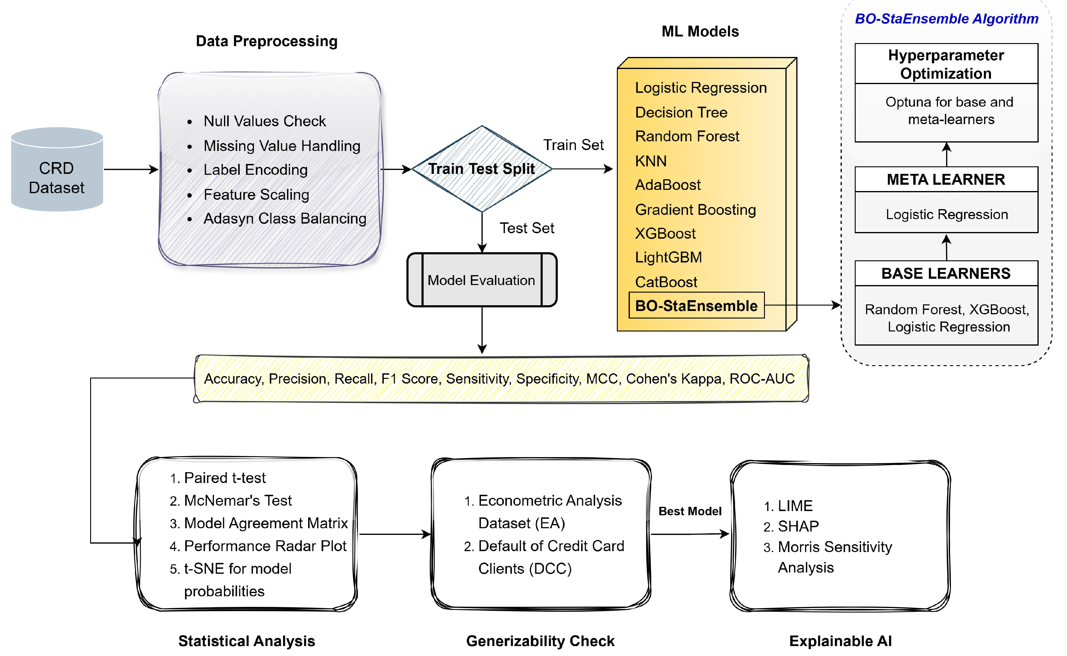
Figure 2.
Class distribution across (a) Credit Risk Dataset (CRD), (b) Econometric Analysis (EA), and (c) Default of credit card clients (DCC).
Figure 2.
Class distribution across (a) Credit Risk Dataset (CRD), (b) Econometric Analysis (EA), and (c) Default of credit card clients (DCC).
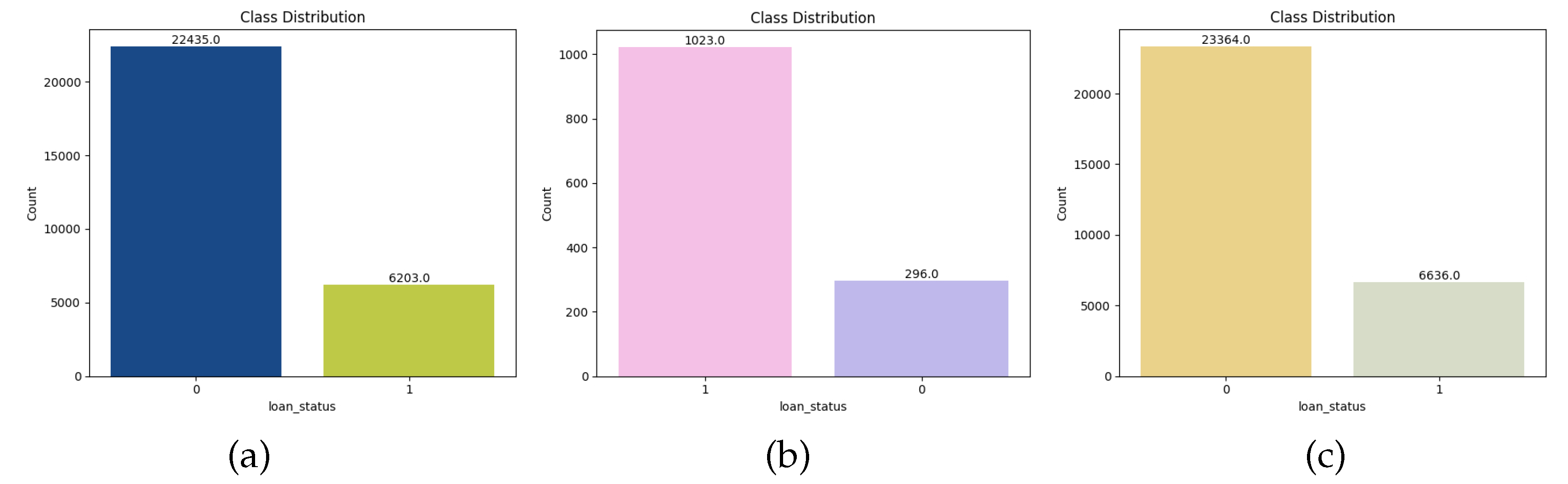
Figure 3.
Class distribution after applying ADASYN across (a) Credit Risk Dataset (CRD), (b) Econometric Analysis (EA), and (c) Default of credit card clients (DCC).
Figure 3.
Class distribution after applying ADASYN across (a) Credit Risk Dataset (CRD), (b) Econometric Analysis (EA), and (c) Default of credit card clients (DCC).
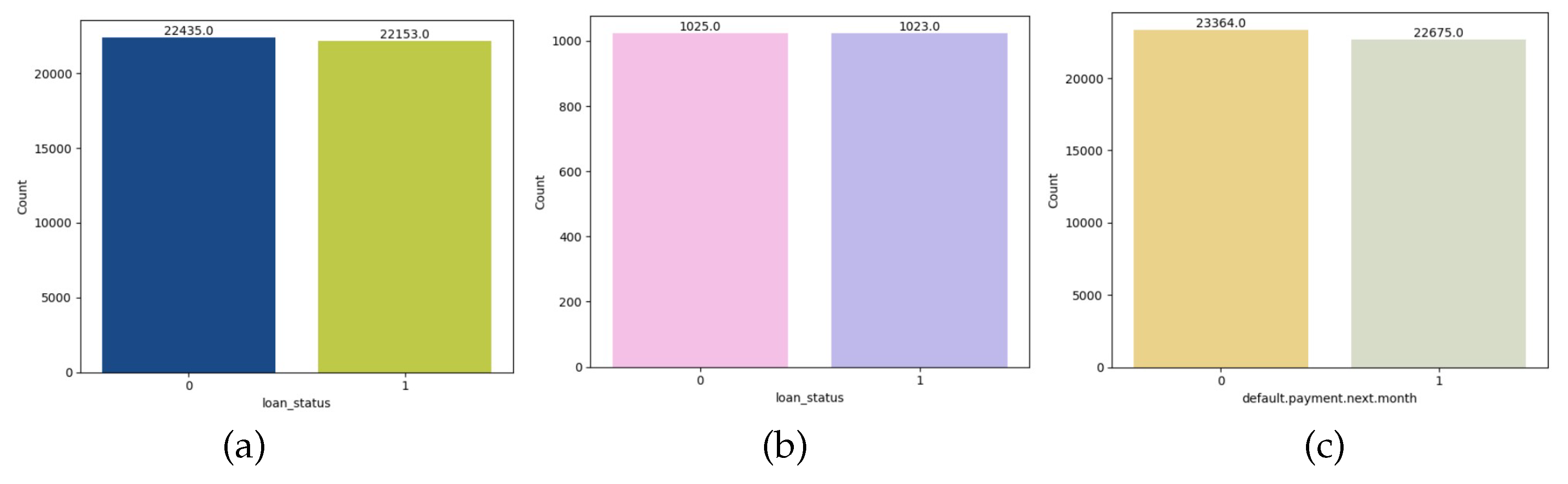
Figure 4.
Correlation Metrics of (a) Credit Risk Dataset (CRD), (b) Econometric Analysis (EA), and (c) Default of credit card clients (DCC).
Figure 4.
Correlation Metrics of (a) Credit Risk Dataset (CRD), (b) Econometric Analysis (EA), and (c) Default of credit card clients (DCC).
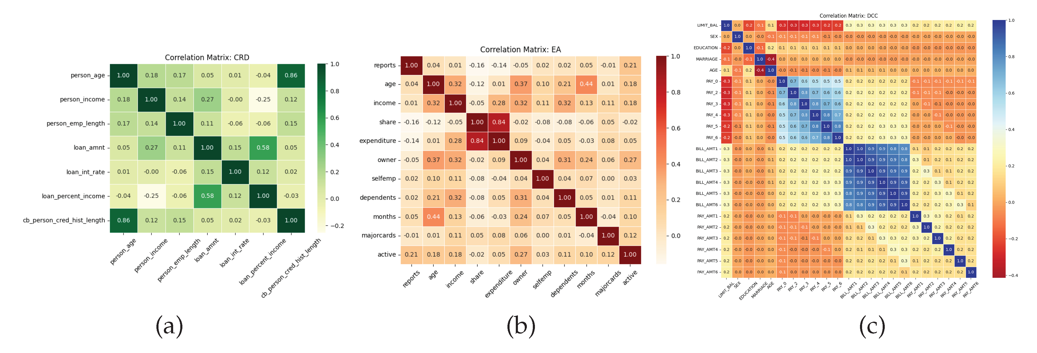
Figure 5.
Confusion Metrics of BO-StaEnsemble approach in (a) Credit Risk Dataset (CRD), (b) Econometric Analysis (EA), and (c) Default of credit card clients (DCC).
Figure 5.
Confusion Metrics of BO-StaEnsemble approach in (a) Credit Risk Dataset (CRD), (b) Econometric Analysis (EA), and (c) Default of credit card clients (DCC).
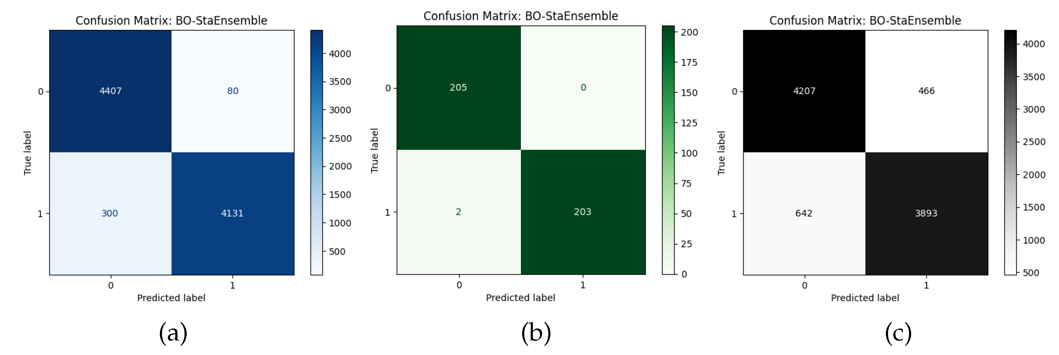
Figure 6.
ROC Curve of BO-StaEnsemble approach in (a) Credit Risk Dataset (CRD), (b) Econometric Analysis (EA), and (c) Default of credit card clients (DCC).
Figure 6.
ROC Curve of BO-StaEnsemble approach in (a) Credit Risk Dataset (CRD), (b) Econometric Analysis (EA), and (c) Default of credit card clients (DCC).
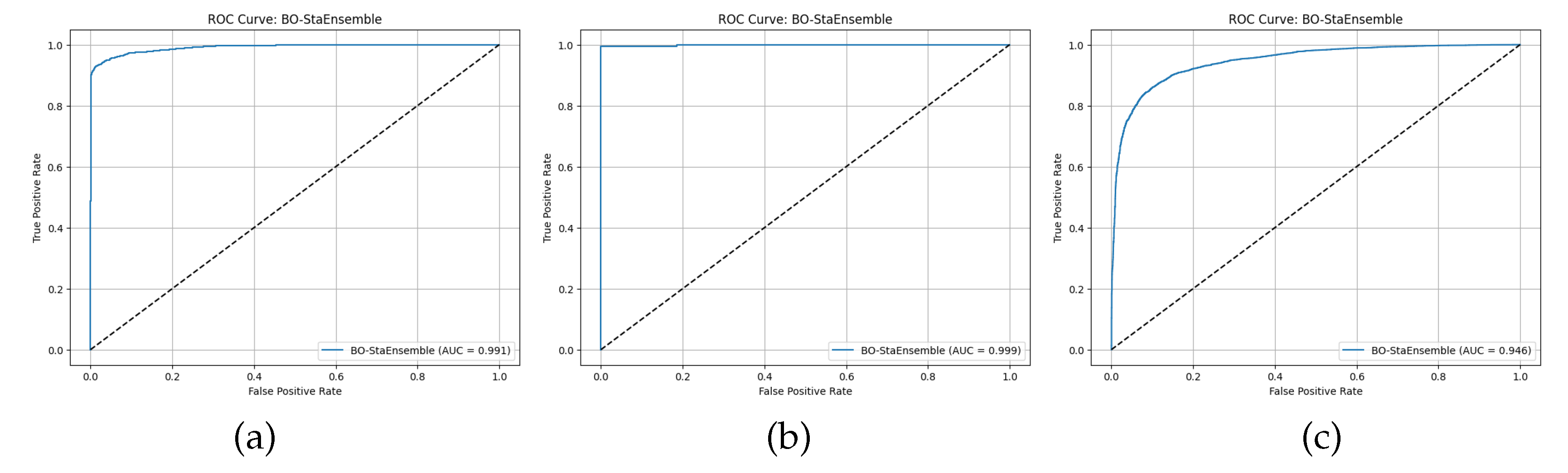
Figure 7.
Radar Plot of BO-StaEnsemble approach in (a) Credit Risk Dataset (CRD), (b) Econometric Analysis (EA), and (c) Default of credit card clients (DCC).
Figure 7.
Radar Plot of BO-StaEnsemble approach in (a) Credit Risk Dataset (CRD), (b) Econometric Analysis (EA), and (c) Default of credit card clients (DCC).
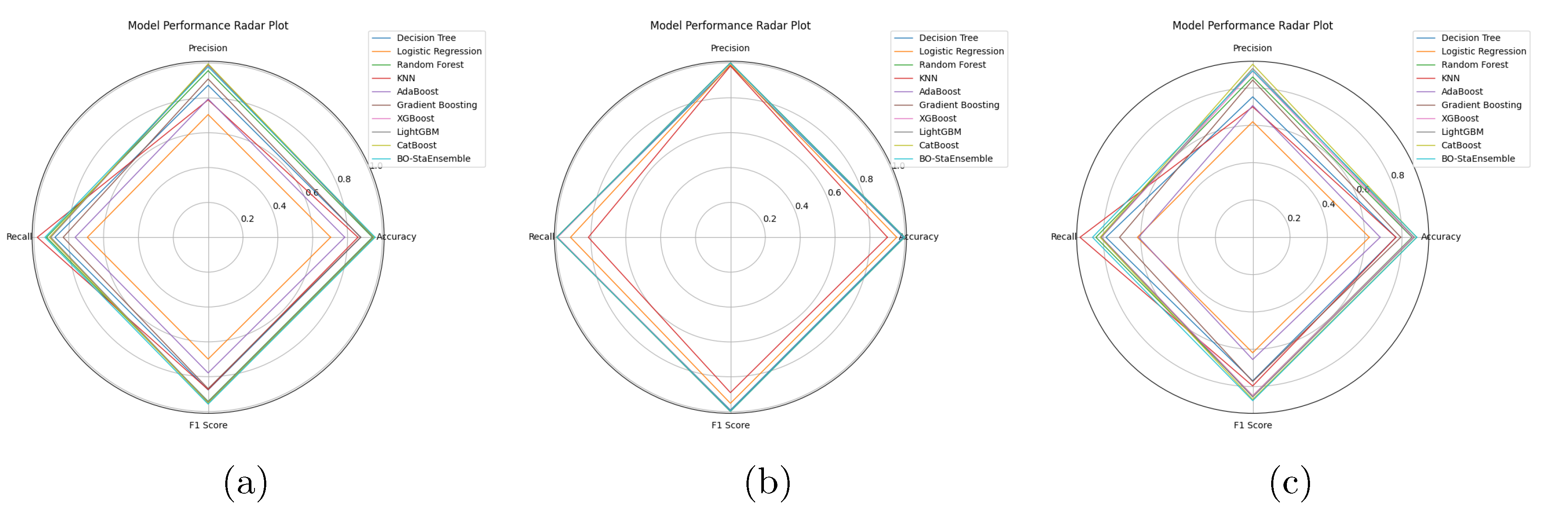
Figure 8.
McNemar’s Test analysis of (a) Credit Risk Dataset (CRD), (b) Econometric Analysis (EA), and (c) Default of credit card clients (DCC).
Figure 8.
McNemar’s Test analysis of (a) Credit Risk Dataset (CRD), (b) Econometric Analysis (EA), and (c) Default of credit card clients (DCC).
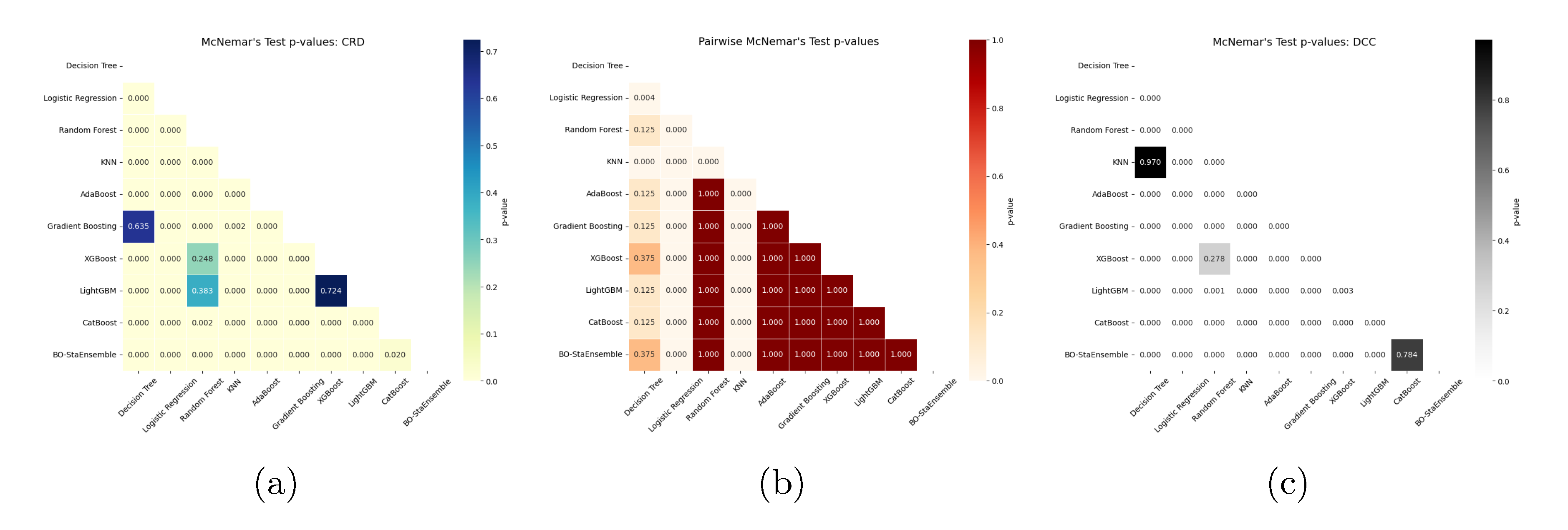
Figure 9.
t-SNE analysis of BO-StaEnsemble approach in (a) Credit Risk Dataset (CRD), (b) Econometric Analysis (EA), and (c) Default of credit card clients (DCC).
Figure 9.
t-SNE analysis of BO-StaEnsemble approach in (a) Credit Risk Dataset (CRD), (b) Econometric Analysis (EA), and (c) Default of credit card clients (DCC).
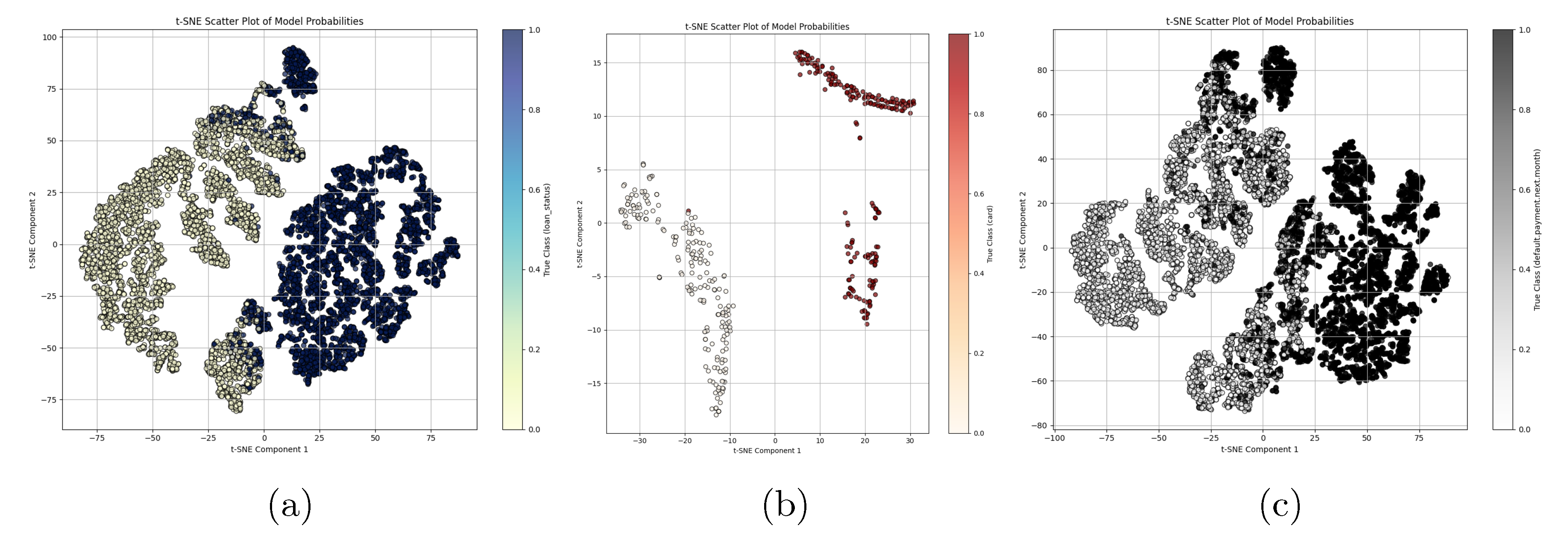
Figure 10.
SHAP (a) and LIME (b) Analysis of Credit Risk Dataset (CRD)
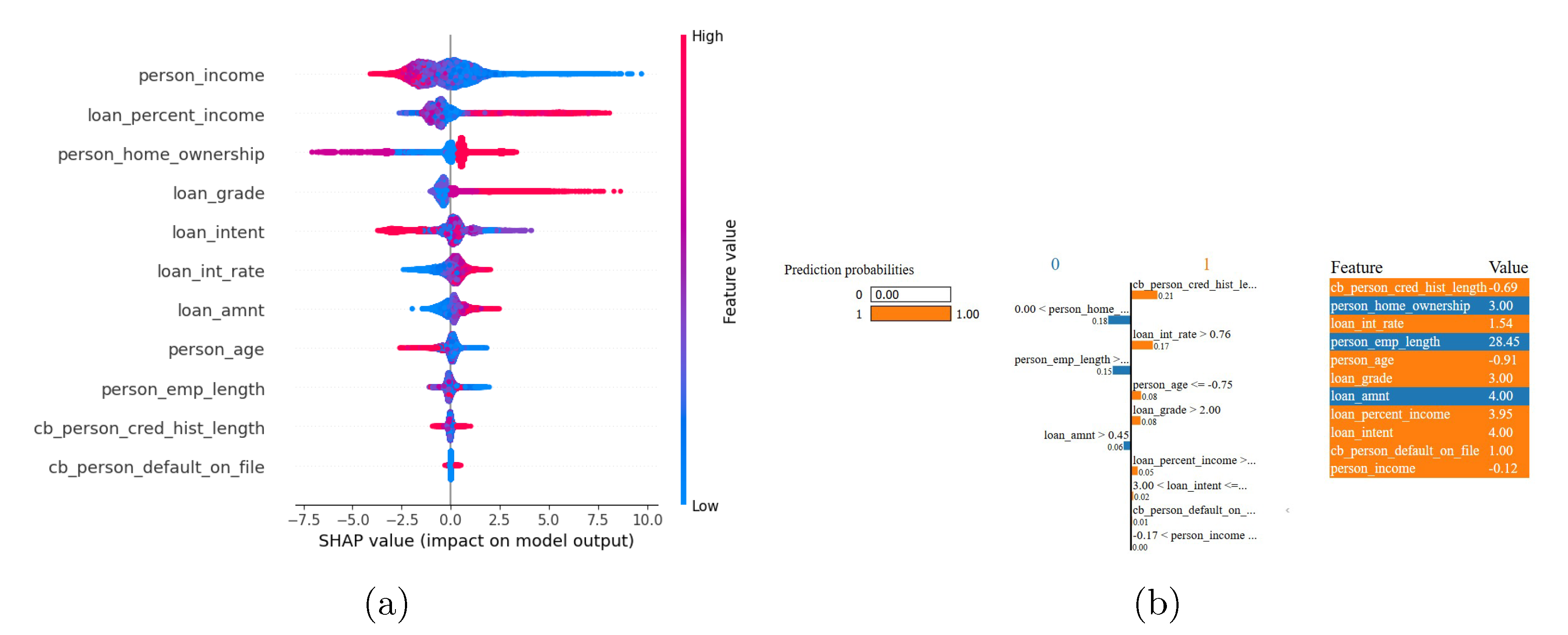
Figure 11.
Morris Sensitivity Analysis of Credit Risk Dataset (CRD).
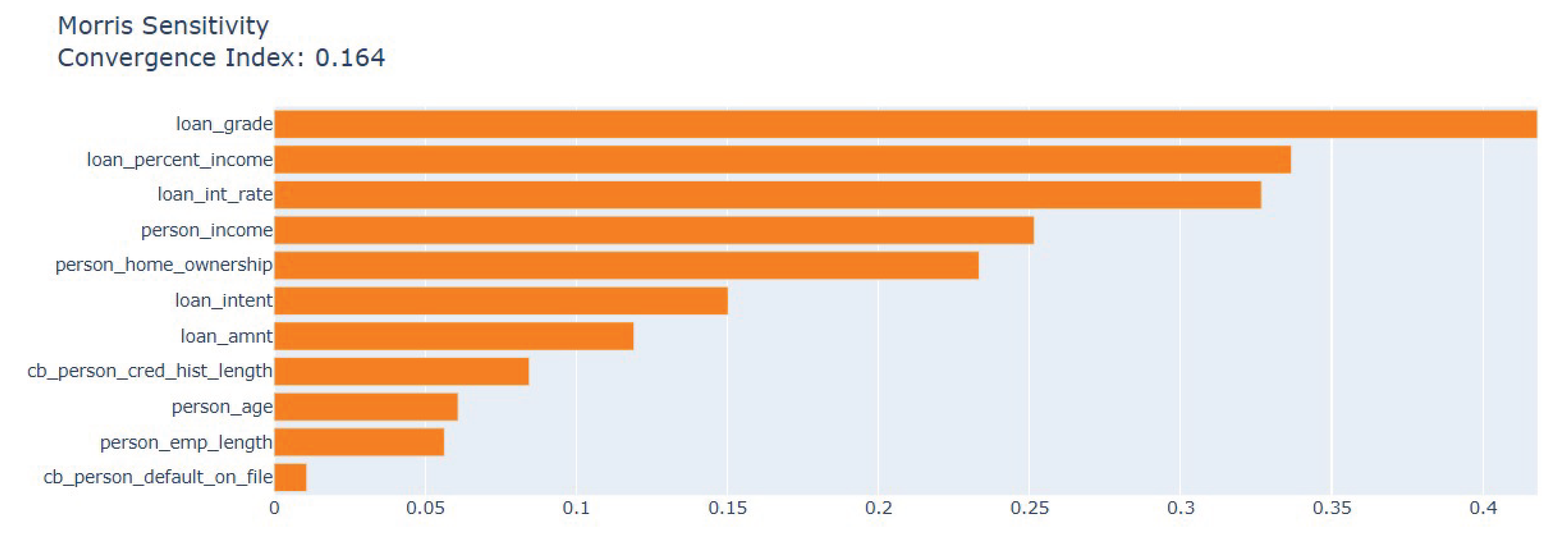
Figure 12.
SHAP (a) and LIME (b) Analysis of Econometric Analysis (EA).
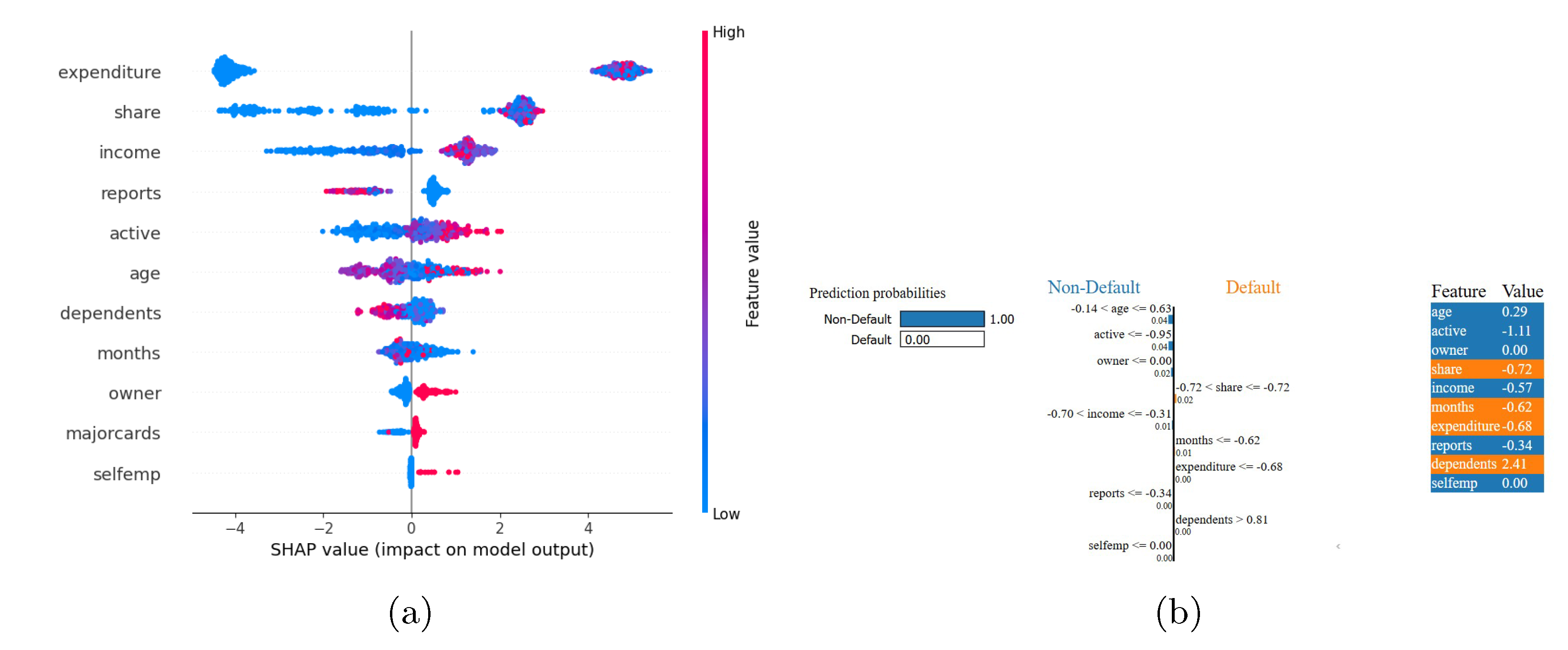
Figure 13.
Morris Sensitivity Analysis of Econometric Analysis (EA).
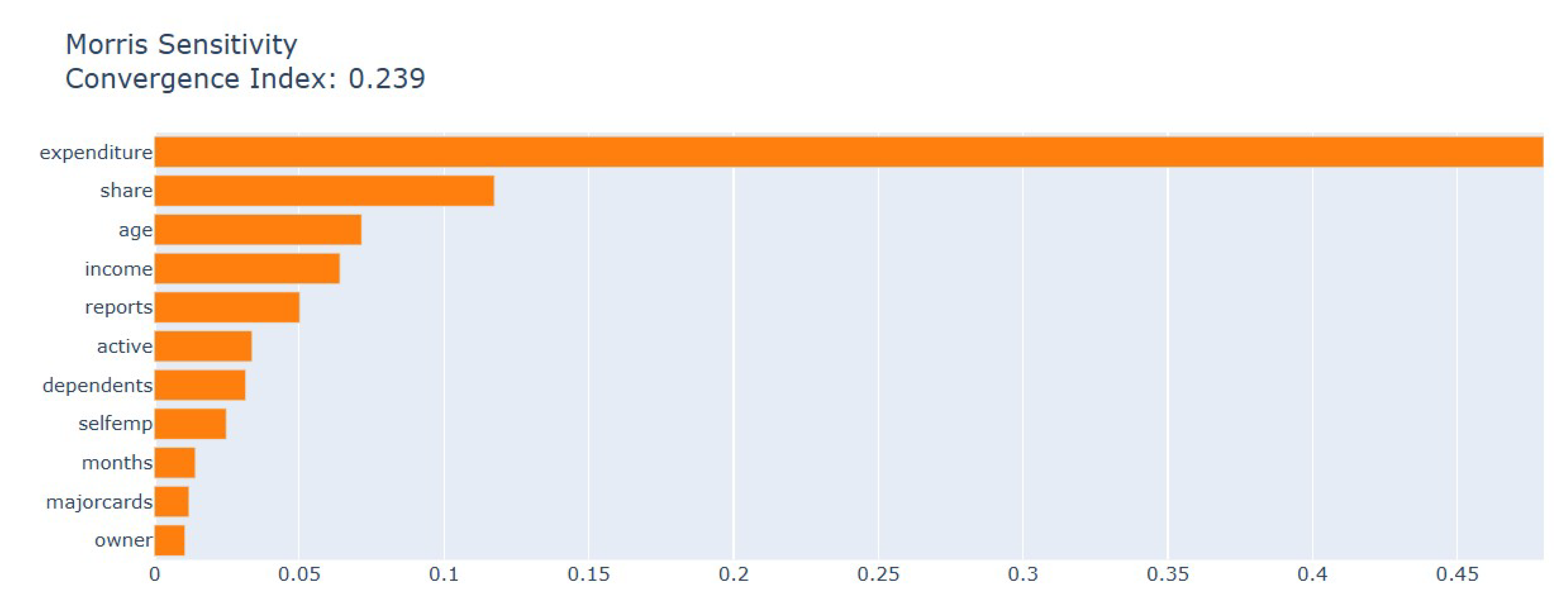
Figure 14.
SHAP (a) and LIME (b) Analysis of Default of credit card clients (DCC).
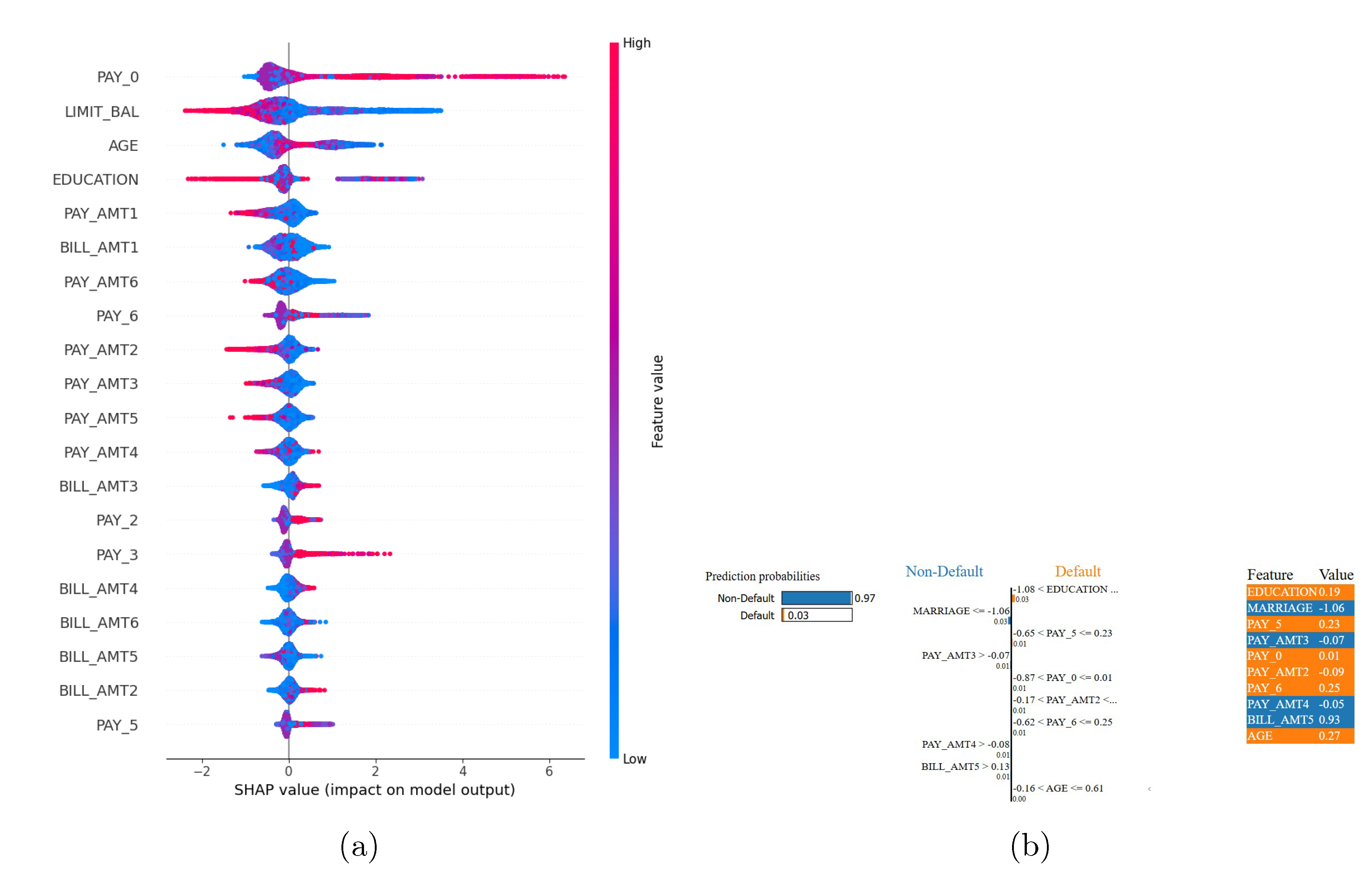
Figure 15.
Morris Sensitivity Analysis of Default of credit card clients (DCC).


Table 1.
Description of the Datasets Used.
| Dataset | Total Instances | Percentage of Defaults | Num of Features | Source |
|---|---|---|---|---|
| Credit Risk Dataset (CRD) | 32,581 | 21.82% | 11 | Kaggle [43] |
| Credit Card Data from ‘Econometric Analysis’ (EA) | 1,319 | 22.44% | 11 | Kaggle [44] |
| Default of credit card clients (DCC) | 30,000 | 22.12% | 23 | UCI [45] |
Table 2.
Hyperparameters for BO-StaEnsemble Components Across Datasets.
| Component | Hyperparameter | CRD | Econometric | DCC |
|---|---|---|---|---|
| Random Forest | n_estimators | 197 | 93 | 146 |
| max_depth | 16 | 11 | 14 | |
| min_samples_split | 9 | 5 | 5 | |
| min_samples_leaf | 1 | 1 | 1 | |
| max_features | sqrt | sqrt | sqrt | |
| XGBoost | n_estimators | 268 | 66 | 278 |
| max_depth | 17 | 6 | 20 | |
| learning_rate | 0.0777 | 0.0798 | 0.0562 | |
| subsample | 0.7569 | 0.7561 | 0.7343 | |
| colsample_bytree | 0.8033 | 0.8407 | 0.9077 | |
| gamma | 0.1 | 0.1 | 0.2 | |
| reg_alpha | 0.01 | 0.01 | 0.05 | |
| Logistic Regression | C | 0.2870 | 0.0252 | 1.1999 |
| penalty | l2 | l2 | l2 | |
| solver | lbfgs | lbfgs | liblinear | |
| Meta-Learner (LR) | C | 0.5677 | 0.1931 | 0.1117 |
| fit_intercept | True | True | True | |
| Bayesian Optimization | Trials | 30 | 30 | 30 |
| Acquisition Function | EI | EI | EI | |
| Initial Points | 10 | 10 | 10 |
sqrt: Square root of total features; EI: Expected Improvement acquisition function.; Default values were applied for non-optimized parameters.
Table 3.
Performance on the Credit Risk Dataset (CRD)
| Model | Accuracy | Sensitivity | Specificity | MCC | Cohen’s |
|---|---|---|---|---|---|
| Decision Tree | 0.8770 | 0.8820 | 0.8721 | 0.7540 | 0.7540 |
| Logistic Regression | 0.7031 | 0.6933 | 0.7127 | 0.4061 | 0.4061 |
| Random Forest | 0.9454 | 0.9318 | 0.9588 | 0.8911 | 0.8908 |
| K-Nearest Neighbour | 0.8597 | 0.9804 | 0.7406 | 0.7418 | 0.7199 |
| AdaBoost | 0.7840 | 0.7635 | 0.8043 | 0.5684 | 0.5679 |
| Gradient Boosting | 0.8749 | 0.8319 | 0.9173 | 0.7522 | 0.7496 |
| XGBoost | 0.9484 | 0.9102 | 0.9862 | 0.8993 | 0.8968 |
| LightGBM | 0.9477 | 0.9030 | 0.9920 | 0.8990 | 0.8954 |
| CatBoost | 0.9534 | 0.9106 | 0.9955 | 0.9099 | 0.9067 |
| BO-StaEnsemble | 0.9600 | 0.9323 | 0.9822 | 0.9159 | 0.9147 |
Table 4.
Performance on the Econometric Analysis Dataset (EA)
| Model | Accuracy | Sensitivity | Specificity | MCC | Cohen’s |
|---|---|---|---|---|---|
| Decision Tree | 0.9878 | 0.9951 | 0.9805 | 0.9757 | 0.9756 |
| Logistic Regression | 0.9537 | 0.9171 | 0.9902 | 0.9098 | 0.9073 |
| Random Forest | 0.9976 | 0.9951 | 1.0000 | 0.9951 | 0.9951 |
| K-Nearest Neighbour | 0.9000 | 0.8146 | 0.9854 | 0.8119 | 0.8000 |
| AdaBoost | 0.9976 | 0.9951 | 1.0000 | 0.9951 | 0.9951 |
| Gradient Boosting | 0.9976 | 0.9951 | 1.0000 | 0.9951 | 0.9951 |
| XGBoost | 0.9951 | 0.9902 | 1.0000 | 0.9903 | 0.9902 |
| LightGBM | 0.9976 | 0.9951 | 1.0000 | 0.9951 | 0.9951 |
| CatBoost | 0.9976 | 0.9951 | 1.0000 | 0.9951 | 0.9951 |
| BO-StaEnsemble | 1.0000 | 0.9902 | 1.0000 | 0.9903 | 0.9902 |
Table 5.
Performance on the Default of Credit Card Clients (DCC)
| Model | Accuracy | Sensitivity | Specificity | MCC | Cohen’s |
|---|---|---|---|---|---|
| Decision Tree | 0.7649 | 0.7837 | 0.7466 | 0.5305 | 0.5300 |
| Logistic Regression | 0.6249 | 0.6183 | 0.6313 | 0.2496 | 0.2496 |
| Random Forest | 0.8572 | 0.8430 | 0.8710 | 0.7144 | 0.7142 |
| K-Nearest Neighbour | 0.7674 | 0.9257 | 0.6137 | 0.5661 | 0.5369 |
| AdaBoost | 0.6831 | 0.6110 | 0.7530 | 0.3681 | 0.3648 |
| Gradient Boosting | 0.7934 | 0.7138 | 0.8707 | 0.5927 | 0.5859 |
| XGBoost | 0.8576 | 0.8106 | 0.9033 | 0.7176 | 0.7148 |
| LightGBM | 0.8654 | 0.8123 | 0.9170 | 0.7342 | 0.7304 |
| CatBoost | 0.8788 | 0.8179 | 0.9379 | 0.7623 | 0.7571 |
| BO-StaEnsemble | 0.8800 | 0.8584 | 0.9003 | 0.7597 | 0.7591 |
Table 6.
Count of statistically significant improvements by BO-StaEnsemble ().
| Dataset | Significant Improvements | Total Comparisons |
|---|---|---|
| CRD | 8/9 | 9 |
| ECA | 2/4 | 4 |
| DCC | 9/9 | 9 |
Disclaimer/Publisher’s Note: The statements, opinions and data contained in all publications are solely those of the individual author(s) and contributor(s) and not of MDPI and/or the editor(s). MDPI and/or the editor(s) disclaim responsibility for any injury to people or property resulting from any ideas, methods, instructions or products referred to in the content. |
© 2025 by the authors. Licensee MDPI, Basel, Switzerland. This article is an open access article distributed under the terms and conditions of the Creative Commons Attribution (CC BY) license (http://creativecommons.org/licenses/by/4.0/).
Copyright: This open access article is published under a Creative Commons CC BY 4.0 license, which permit the free download, distribution, and reuse, provided that the author and preprint are cited in any reuse.


