
Submitted:
15 May 2025
Posted:
16 May 2025
You are already at the latest version
Abstract
Small and Medium Enterprises (SMEs) often face challenges in obtaining credit due to their per-ceived high credit risk. This study aims to develop a deep learning model using the stacking ensemble technique to enhance the accuracy of credit risk assessment for SMEs. The research utilizes a dataset from the Ministry of Industry, consisting of 14 quantitative and qualitative variables. Due to data imbalance, four data balancing techniques are applied: Synthetic Minority Over-sampling Technique (SMOTE), Adaptive Synthetic Sampling (ADASYN), a combination of SMOTE and Edited Nearest Neighbors (SMOTEENN), and a combination of SMOTE and Tomek Links (SMOTETomek). The study compares the performance of nine machine learning models: Decision Tree, Support Vector Machines (SVM), Gradient Boosting, K-Nearest Neighbors (KNN), Naïve Bayes, Logistic Regression with Meta-Learning, Gradient Boosting with Meta-Learning, Extreme Gradient Boosting with Meta-Learning, and Multi-layer Perceptron Neural Network with Meta-Learning. Model performance is evaluated based on Accuracy, Precision, Recall, F1-score, and Area Under the ROC Curve (AUCs). Results indicate that the stacking ensemble technique, particularly the Multi-layer Perceptron Neural Network with Meta-Learning, achieves the highest performance, with an F1-score of 0.953 and an AUCs of 0.990. Logistic Regression with Meta-Learning and Gradient Boosting with Meta-Learning also yield strong results, outper-forming baseline models such as standard Gradient Boosting. Furthermore, applying Stepwise Feature Selection reduces the number of variables without compromising model performance. Overall, the combination of stacking ensemble models, data balancing techniques, and optimal feature selection significantly enhances the accuracy of credit risk assessment for SMEs.
Keywords:
credit risk models
; decision tree
; support vector machine
; logistic regression
; adaptive boosting model
; AdaBoost
; NPL
; status of installment payments
; creditworthiness
; stacking ensemble technique
1. Introduction
Small and medium-sized enterprises (SMEs) are pivotal in driving the global economy through job creation and the stimulation of economic growth [1,2]. However, SMEs often encounter challenges in securing credit from financial institutions due to their perceived higher credit risk, particularly during economic downturns or crises such as the COVID-19 pandemic, which can lead to reduced revenue while operational costs remain relatively fixed [3,4]. These financial constraints elevate the risk of business closures, compelling SMEs to seek external funding sources more frequently [5]. In response to the potential for increased Non-Performing Loans (NPLs), financial institutions have tightened their lending criteria, underscoring the need for more accurate and unbiased Credit Risk Assessment (CRA) methodologies [6,7]. In this context, machine learning (ML) has emerged as a promising tool for analyzing borrower data, enabling financial institutions to assess the creditworthiness of SMEs more efficiently and with greater impartiality [8,9], thereby potentially balancing effective risk management with enhanced access to credit for viable businesses [10].
Our prior work [11] directly addressed the challenges associated with credit risk assessment for SMEs through a series of investigations leveraging machine learning techniques. In particular, [12] conducted a comparative study of several fundamental classification algorithms, emphasizing the performance improvements achieved through data balancing methods—most notably the Synthetic Minority Over-sampling Technique (SMOTE). This study highlighted the potential of Gradient Boosting in enhancing prediction outcomes once class imbalance was effectively addressed. These earlier investigations collectively underscored two critical challenges in SME credit risk modeling: the difficulty in attaining high predictive performance and the pronounced impact of class imbalance inherent in credit datasets.
In this article, we focus on developing a machine learning model utilizing the Stacking ensemble technique to analyze 14 key factors associated with credit risk. The dataset comprises secondary data obtained from the Ministry of Industry, encompassing variables such as the applicant's age (Age), the number of family or business members involved in the loan request (Member), incoming business debt (IN_debt), outgoing business debt (OUT_debt), number of employees (Num_Emp), annual expenses (Expenses_Y), the ratio of new customers to total customers (ratio_CCus/TCus), the business growth rate over three years (Growth_rate_3Y), net income from the previous year (Net_income_LY), incoming debt specifically from business operations (IN_debt_Bus), outgoing debt specifically from business operations (OUT_debt_Bus), the loan amount requested from financial institutions (Loan_Amount), the loan term (period), and the target variable (Target: 0 = non-NPL, 1 = NPL) [13]. To address the class imbalance between default and non-default cases, four resampling techniques are applied: SMOTE, Adaptive Synthetic Sampling (ADASYN), SMOTE-Edited Nearest Neighbors (SMOTEENN), and SMOTE-Tomek Links (SMOTETomek), which are known to enhance classification performance [14,15].
The study compares the performance of nine distinct models: Decision Tree, Support Vector Machine (SVM), Gradient Boosting, K-Nearest Neighbors (KNN), Naïve Bayes, a meta-classifier using Logistic Regression, a meta-classifier using Gradient Boosting, a meta-classifier using Extreme Gradient Boosting (XGBoost), and a meta-classifier using a Multi-layer Perceptron (MLP) Neural Network [16,17]. Performance evaluation will be based on metrics including Accuracy, Precision, Recall, F1-score, and the Area Under the Receiver Operating Characteristic Curve (AUC). The computational analysis is conducted using Google Colaboratory [18].
2. Materials and Methods
2.1. Data
2.1.1. Data Acquisition
To analyze the borrower database of the Revolving Fund from the Fund for the Promotion of Household Industry and Handicrafts (FPHIH), operating under the Department of Industrial Promotion (DIP), Ministry of Industry, Thailand, this study utilizes data specifically focused on individual borrowers. While the dataset contains records for both individual and legal entity borrowers, the present study concentrates exclusively on individuals, as they represent the primary customer group and account for a substantial share of Non-Performing Loan (NPL) cases. The FPHIH provides financial support to community-level entrepreneurs and craftspeople nationwide, aiming to strengthen grassroots economic resilience through accessible credit schemes.
The selection of variables was guided by their relevance to prior research and data completeness. Variables with a high proportion of missing values were excluded to maintain analytical integrity. Data consistency was verified, and outliers were carefully examined and treated as necessary to enhance data quality. Table 1 and Table 2 present the selected features and their descriptive statistics, respectively, while Figure 1 provides a pairwise visualization of the numerical variables included in the analysis.
The dataset includes 1,014 individual borrower records, consisting of 742 non-NPL cases (approximately 73.2%) and 272 NPL cases (approximately 26.8%). This distribution reveals a significant class imbalance, which poses challenges for classification algorithms and necessitates special handling during model development. Techniques such as oversampling, undersampling, and Synthetic Minority Oversampling Technique (SMOTE) will be employed in subsequent stages to address this imbalance and improve model performance.
2.1.2. Data Exploration
To examine the distribution of each variable and explore potential relationships among features, a pair plot was generated, as shown in Figure 1. This graphical representation displays scatter plots for all possible combinations of numerical variables, with each diagonal element illustrating the univariate distribution of a corresponding feature. This enables a clear view of the data structure, including skewness, clustering, and potential outliers.

Table 1.
Variable Names from the Fund for the Promotion of Household Industry and Handicrafts of Thailand.
Table 1.
Variable Names from the Fund for the Promotion of Household Industry and Handicrafts of Thailand.
| Variable name | Description |
| Age | Age (years) at the time of loan application. |
| Member | Number of family members at the time of loan application. |
| IN_debt | Total debt with all formal financial institutions that are not related to business at the time of loan application. |
| OUT_debt | Total amount of informal debt that is not related to business at the time of loan application. |
| Num_Emp | Number of employees. |
| Exprenses_Y | Expenses per year (Baht). |
| Ratio_CCus-TCus | Rate of change in total employee expenses during the 3 years before the time of loan application (%). |
| Growth_rate_3Y | Average annual growth rate of income for the past 3 years at the time of loan application (% per year). |
| Net-income_LY | Last year's net profit rate at the time of loan application (%). |
| IN_debt_BUS | The total amount of debt borrowed from financial institutions in the system for use in business at the time of loan application. |
| OUT_debt_BUS | Total debt of informal loans borrowed for use in business at the time of loan application. |
| Loan_Amount | The loan amount received at the time of loan application. |
| period | The period for repaying the loan at the time of loan application. |
| Target (Dependent variable) | Current installment payment status. |
Table 2.
Descriptive Statistics.
| Variable name | Mean | SD | Median | Max | Min |
| Age | 44.62 | 9.87 | 45.00 | 74.00 | 20.00 |
| Member | 1.21 | 1.30 | 1.00 | 10.00 | 0.00 |
| IN_debt | 587,794.00 | 1,280,888.00 | 144,835.00 | 19,834,280.00 | 0.00 |
| OUT_debt | 16,617.84 | 257,638.80 | 0 | 7,214,728.00 | 0.00 |
| Num_Emp | 6.56 | 9.31 | 4.00 | 201.00 | 0.00 |
| Exprenses_Y | 708,148.10 | 904,281.70 | 520,000.00 | 18,540,000.00 | 0.00 |
| Ratio_CCus-TCus | 52.36 | 23.38 | 50.00 | 225.00 | 0.00 |
| Growth_rate_3Y | 21.38 | 18.41 | 20.00 | 100.00 | -10.00 |
| Net-income_LY | 23.51 | 17.15 | 20.00 | 100.00 | -60.00 |
| IN_debt_BUS | 407,685.90 | 1,033,702.00 | 0.00 | 19,834,280.00 | 0.00 |
| OUT_debt_BUS | 2,393.02 | 43,475.00 | 0.00 | 1,300,000.00 | 0.00 |
| Loan_Amount | 253,024.70 | 650,243.40 | 200,000.00 | 20,000,000.00 | 0.00 |
| period | 56.70 | 16.50 | 60.00 | 116.00 | 0.00 |
This visualization not only supports the detection of data irregularities but also serves as a foundation for identifying redundant variables and guiding feature selection for the predictive modeling phase.
The pair plot reveals various levels of interaction between variables. For example, the variable Growth_rate_3Y exhibits a significantly skewed distribution, indicating that most borrowers experienced low to moderate growth, with a few outliers achieving substantially higher growth. Similarly, Ratio_CCus.TCus and Period show distinct value ranges that may reflect differences in borrower behavior or loan structure. Some variable pairs exhibit weak to moderate linear relationships, suggesting the potential for multicollinearity, which could affect model interpretability.
2.2. Feature Selection and Multicollinearity Diagnosis
2.2.1. Stepwise Selection Method
Feature selection plays a critical role in improving model generalizability, especially when working with a moderate number of input variables. In this study, Stepwise Selection was chosen due to its balance between simplicity and effectiveness, particularly in datasets where statistical relationships exist among variables. This method systematically adds (Forward Selection) and removes (Backward Elimination) features based on statistical criteria, optimizing model performance by retaining only the most informative predictors while reducing unnecessary complexity.
2.2.2. Generalized Linear Model (GLM) Results
The feature selection process was conducted using R, applying stepwise procedures on a Generalized Linear Model (GLM) with the binary target variable (NPL or non-NPL). The model identified the following variables as statistically significant: Age, Member, Num_Emp, Ratio_CCus.TCus, Growth_rate_3Y, Net.income_LY, Period These predictors were retained for further modeling, and their regression coefficients and significance levels are presented in Table 3
2.2.3. Variance Inflation Factor (VIF) Analysis
To assess the degree of multicollinearity among the selected predictors, the Variance Inflation Factor (VIF) was computed for each variable. Multicollinearity can distort the estimation of regression coefficients and undermine model reliability. The VIF results, as shown in Table 4, confirm that all included variables exhibit acceptable levels of multicollinearity (VIF < 5), consistent with standard statistical thresholds.
This indicates that the model’s coefficients are interpretable and statistically robust, forming a reliable foundation for subsequent machine learning-based classification tasks.
2.3. Machine Learning Models and Algorithms
2.3.1. Decision Trees
Decision Trees are non-parametric, supervised learning models used for both classification and regression. These models operate by recursively splitting the data based on feature values, resulting in a tree-like structure where each internal node represents a decision rule, each branch corresponds to an outcome of the rule, and each leaf node signifies a predicted class or value. The model learns to approximate the target function in a piecewise constant manner, enabling it to capture simple nonlinear patterns in the data. Decision trees are particularly interpretable and require minimal data preprocessing [19,20].
2.3.2. Support Vector Machine (SVM)
Support Vector Machines are robust supervised learning algorithms particularly effective for classification tasks in high-dimensional spaces. SVMs identify the optimal separating hyperplane that maximizes the margin between data points of different classes. The classification of new data points is determined based on their distance from this hyperplane. Furthermore, by employing kernel functions, SVMs can efficiently handle non-linearly separable data by implicitly mapping it into higher-dimensional feature spaces. Their ability to generalize well and tolerate outliers makes them a reliable choice for various complex tasks [21,22,23,24].
2.3.3. Adaptive Boosting Model (AdaBoost)
AdaBoost, short for Adaptive Boosting, is an ensemble technique that constructs a strong classifier by combining several weak learners, often shallow decision trees (also known as decision stumps). During training, AdaBoost iteratively adjusts the weights of incorrectly classified instances, forcing subsequent learners to focus more on challenging cases. This adaptive nature enhances the model’s overall accuracy and robustness. The final prediction is made through a weighted majority vote of all learners. For implementation specifics and theoretical foundations, see [25].
2.3.4. K-Nearest Neighbors (KNN) Classification Method
K-Nearest Neighbors is a lazy learning algorithm based on the assumption that similar data instances exist in close proximity. When classifying a new sample, the algorithm computes its distance (commonly Euclidean or Manhattan) to all points in the training dataset and selects the ‘k’ closest neighbors. The class most frequent among these neighbors determines the predicted label. KNN is straightforward and non-parametric, making it useful for exploratory analysis, but it can become computationally expensive and memory-intensive, particularly with large datasets or high-dimensional features [26,27].
2.3.5. Naïve Bayes
Naïve Bayes classifiers are probabilistic models based on Bayes' Theorem with the simplifying assumption that input features are conditionally independent given the class label. Despite this strong assumption, Naïve Bayes often performs well in practice, especially in high-dimensional settings such as text classification and spam detection. The classifier computes posterior probabilities for each class and assigns the class label with the highest probability. Its efficiency, scalability, and interpretability make it an attractive option for large-scale classification problems [28,29,30,31].
2.3.6. Logistic Regression
Logistic regression is a statistical method commonly applied to binary classification tasks. It models the relationship between a set of independent variables and a binary dependent variable using the logistic function (sigmoid), which maps linear combinations of inputs into probability estimates between 0 and 1. This probability can be interpreted as the likelihood of an event occurring (e.g., Y = 1 for success, Y = 0 for failure). Logistic regression is widely used due to its interpretability, ease of implementation, and ability to handle both numerical and categorical predictors [32,33].
2.3.7. Gradient Boosting
Gradient Boosting is an advanced ensemble learning method that combines multiple weak learners—typically decision trees—into a strong predictive model. It operates in a sequential manner, where each model attempts to correct the residual errors of its predecessor. Optimization is performed through gradient descent on a chosen loss function, allowing the model to iteratively minimize prediction error. Gradient Boosting is highly effective in capturing complex data patterns and is extensively used in domains such as financial forecasting, medical diagnosis, and fraud detection due to its superior accuracy and flexibility [34,35,36,37,38].
2.3.8. Multi-Layer Perceptron Neural Network
A Multi-layer Perceptron is a type of artificial neural network composed of an input layer, one or more hidden layers, and an output layer. Each neuron processes inputs through weighted connections and nonlinear activation functions, and the network is trained via backpropagation to minimize a loss function. The MLP is capable of approximating complex, non-linear functions, making it suitable for a wide range of prediction tasks. An enhanced version, META-MLP, incorporates meta-learning techniques that optimize hyperparameters and improve performance across diverse datasets. This approach is particularly advantageous in domains requiring robust generalization, such as financial modeling and time series prediction [39,40,41,42].
2.4. Confusion Matrix and Evaluation Metrics
2.4.1. Confusion Matrix
The confusion matrix is a foundational tool used to visualize and assess the performance of a classification model by comparing predicted outcomes against actual values. It provides a summary of prediction results in terms of four distinct categories:
Table 5.
Confusion matrix.
| Actual | |||
|---|---|---|---|
| Positive | Negative | ||
| Predicted | Positive | True Positive (TP) | False Positive (FP) |
| Negative | False Negative (FN) | True Negative (TN) | |
- -
- True Positive (TP): Instances where the model correctly predicts the presence of the positive class.
- -
- True Negative (TN): Instances where the model correctly predicts the absence of the positive class (i.e., the negative class).
- -
- False Positive (FP): Cases where the model incorrectly predicts the positive class when the actual class is negative. This is also referred to as a Type I error.
- -
- False Negative (FN): Cases where the model fails to identify the positive class and instead predicts it as negative. This is also known as a Type II error.
These components are arranged in a matrix form, facilitating the computation of various performance metrics and enabling a structured evaluation of model efficacy [43]. In this study, we apply standard performance measures derived from the confusion matrix, including accuracy, precision, recall, F-measure, and the Receiver Operating Characteristic (ROC) curve, to evaluate the predictive power of our classification models [44].
2.4.2. Accuracy
Accuracy is one of the most commonly used evaluation metrics in classification tasks. It is defined as the proportion of correct predictions (both true positives and true negatives) among the total number of predictions. Mathematically, it is expressed as:
While widely adopted, accuracy may be misleading in imbalanced datasets where the number of instances in each class differs significantly.
2.4.3. Precision
Precision measures the proportion of correctly identified positive instances among all instances that were predicted as positive. It reflects the reliability of positive predictions made by the model and is calculated as:
A high precision indicates a low false positive rate, making it a valuable metric in contexts where false alarms are costly.
2.4.4. Recall
Recall evaluates the model's ability to correctly identify all relevant instances of the positive class. It measures the proportion of actual positives that were correctly predicted, as given by:
This metric is critical in applications where missing a positive instance (i.e., a false negative) has severe consequences, such as in medical diagnosis or fraud detection.
2.4.5. F-Measure
The F-measure, or F1-score, combines precision and recall into a single metric by computing their harmonic mean. It provides a balanced evaluation, particularly useful when there is a trade-off between precision and recall:
The F1-score is especially informative in imbalanced classification scenarios, offering a more nuanced view of model performance than accuracy alone.
2.4.6. The Receiver Operating Characteristic (ROC) Curve
The ROC curve is a graphical representation used to assess the performance of a binary classifier across various discrimination thresholds. It plots the True Positive Rate (Recall) against the False Positive Rate (1 - Specificity). The curve illustrates the trade-off between sensitivity and specificity, providing insight into the model's discriminative ability. The Area Under the Curve (AUC) is often used as a scalar measure of this performance, where a value closer to 1 indicates better classification capability.
2.5. Experiments
2.5.1. Development of the Stacking Model with Balanced Data
This study focuses on enhancing the performance of credit risk assessment by applying a two-step model combination technique known as Stacked Generalization or Stacking. This approach integrates multiple models to strengthen their individual predictive capabilities. The original dataset exhibits a significant class imbalance between NPL (Non-Performing Loans) and Non-NPL instances, which can bias model training and reduce accuracy in detecting the minority class.
The overall workflow of the model development and evaluation process is illustrated in Figure 2. It outlines the end-to-end steps from data loading and preprocessing to the generation of base/meta features and final performance evaluation.
To mitigate the class imbalance issue, four data balancing techniques were applied:
- (1)
- SMOTE (Synthetic Minority Oversampling Technique): Generates synthetic samples to increase the representation of NPL cases to balance with Non-NPL
- (2)
- ADASYN (Adaptive Synthetic Sampling Approach): Focuses on generating synthetic data near decision boundaries, helping the model learn more complex patterns.
- (3)
- SMOTEENN or SMOTE + ENN (Edited Nearest Neighbors): A hybrid technique that combines SMOTE to oversample the minority class with ENN, which removes ambiguous instances based on their neighborhood consistency. ENN filters out majority class samples (and occasionally noisy minority ones) that conflict with their nearest neighbors, helping to reduce class overlap and improve decision boundary clarity.
- (4)
- SMOTETomek or SMOTE + Tomek Links: A hybrid method combining SMOTE for oversampling and Tomek Links to remove borderline instances.
Stacking leverages the strengths of multiple base models by combining their outputs into a second-level learner, thereby reducing individual model bias and variance. This hierarchical learning structure enhances generalization by capturing diverse decision boundaries from heterogeneous learners.
2.5.1.1. Data Splitting and Cross-Validation
The balanced dataset was split into a training set and a test set using an 80:20 ratio via stratified sampling to maintain class proportions. The test set remained untouched during the cross-validation process and was used solely for the final evaluation of the trained ensemble model.
Model performance was evaluated using Stratified K-Fold Cross-Validation (K=5) on the training set to ensure model stability and reduce variance in evaluation results.
Five base models were selected and trained:
- (1)
- Decision Tree.
- (2)
- Support Vector Machine (SVM).
- (3)
- Gradient Boosting.
- (4)
- K-Nearest Neighbors (KNN)
- (5)
- Naïve Bayes
Each model was trained on different folds of the data and produced probability estimates for each class, which were then used as new features in the next stage. Using probabilities instead of hard class labels allows the meta-model to capture nuanced differences and model uncertainty more effectively.
2.5.1.2. Training the Meta-Model
The predicted probabilities from the base learners were used as input features for training the meta-model. This approach enables the meta-learner to capture uncertainty and subtle differences in model predictions, leading to improved final classification.
Multiple meta-models were tested to evaluate their effectiveness in combining base model outputs:
- (1)
- Logistic Regression was selected as a baseline meta-model due to its interpretability and computational efficiency.
- (2)
- Gradient Boosting and XGBoost (Extreme Gradient Boosting) were included for their strong ensemble capabilities and ability to handle non-linear relationships via gradient-based optimization.
- (3)
- Multilayer Perceptron (MLP) was incorporated to explore non-linear decision boundaries through deep learning, as it can model complex interactions between input features.
2.5.1.3. Model Evaluation and Conclusion
Model performance was evaluated using the average metrics from Stratified K-Fold Cross-Validation (K=5). The key performance indicators included Accuracy, Precision, Recall, F1-Score, and AUC-ROC to measure classification performance across both NPL and Non-NPL classes.
All performance metrics were calculated per fold and averaged using the macro average strategy to ensure balanced evaluation across both classes, regardless of their frequency in the dataset.
3. Results
This study aimed to develop a learning model using the Stacking technique to analyze key factors associated with credit risk. A total of 14 factors were considered using secondary data obtained from the Ministry of Industry. The dataset was balanced using four techniques: SMOTE, ADASYN, SMOTEENN, and SMOTETomek. The performance of nine predictive methods was compared: Decision Tree, Support Vector Machine (SVM), Gradient Boosting, K-Nearest Neighbors (KNN), Naïve Bayes, Improved Logistic Regression, Improved Gradient Boosting, Improved Extreme Gradient Boosting, and Multilayer Perceptron Neural Network. Model performance was evaluated using Accuracy, Precision, Recall, F-measure, and Area Under the ROC Curve (AUC).
These metrics were selected due to their ability to capture classification performance under class imbalance. Particularly, F1-score reflects a trade-off between Precision and Recall, while AUC evaluates the model’s ability to discriminate between the two classes across all thresholds.
Compared to the baseline accuracy of 0.734—achieved by predicting the majority class only—the stacking-based models showed substantial improvement in both detection of the minority class and overall balance of performance metrics.
The entire model development process, including resampling, cross-validation, and stacking, is visualized in Figure 2 for clarity and reproducibility.
3.1. Results of Stacking-Based Learning Models
The original dataset used in this study was imbalanced. The target variable had two classes: Class 0 (Non-NPL) with 742 instances and Class 1 (NPL) with 272 instances, showing a significant imbalance that could lead to model overclassification toward the majority class, as illustrated in Figure 3.
To address the class imbalance issue, four resampling methods were applied: SMOTE, ADASYN, SMOTE+ENN, and SMOTE+Tomek. The outcomes are shown in Table 6 and Figure 4. After balancing, SMOTE+ENN not only increased the sample size for the minority class but also removed potentially confusing instances, which helped improve model performance. The effectiveness of each technique varies depending on the nature of the data and the objective of analysis.
The study implemented the Stacking technique to enhance model performance by combining base learners. These models were trained on resampled datasets using SMOTE, ADASYN, SMOTEENN, and SMOTETomek. Evaluation metrics included Accuracy, Precision, Recall, F-measure, and AUC.
The base models were selected to cover a variety of learning biases: Decision Tree for interpretability, SVM for margin-based classification, Gradient Boosting for capturing non-linear interactions, KNN for instance-based learning, and Naïve Bayes for probabilistic modeling.
The stacking-based meta-learners—META-LR, META-GB, META-XGB, and META-MLP—demonstrated improved performance across all metrics, with better balance between Recall and Precision compared to base models, as shown in Table 7, Table 8, Table 9 and Table 10.
Logistic Regression was selected as a baseline meta-model due to its interpretability and efficiency, while Gradient Boosting and XGBoost provide powerful ensemble capabilities with gradient optimization. The Multilayer Perceptron (MLP) was included to explore non-linear decision boundaries through deep learning. The outputs used for training the meta-model were probability estimates from each base model rather than discrete class labels. This approach enables the meta-learner to capture uncertainty and subtle differences in model predictions, leading to improved final classification.
All reported performance metrics represent the average values across five folds using Stratified K-Fold Cross-Validation to ensure robust and unbiased evaluation. The test set remained untouched during the cross-validation process and was used solely for the final evaluation of the trained ensemble model.
Under SMOTE, meta-models consistently outperformed traditional base models across all evaluation metrics. META-MLP and META-LR achieved the highest Accuracy (0.808 and 0.805) and AUC (0.890), with full feature sets providing a better balance between Precision and Recall. In contrast, stepwise selection enhanced performance in META-GB, improving Accuracy to 0.795 and AUC to 0.850. Among base models, stepwise selection notably improved Recall and AUC for Decision Tree, SVM, and Naïve Bayes. Despite lower Precision, these models demonstrated enhanced sensitivity. Overall, meta-models under SMOTE showed strong robustness, particularly when combined with full feature sets.
Under ADASYN, meta-models outperformed base models across all performance metrics. META-MLP and META-LR full models achieved the highest Accuracy (0.831 and 0.814), F-measure (0.837 and 0.814), and AUC (0.910 and 0.900), demonstrating a strong balance between Precision and Recall. Stepwise selection slightly improved META-GB’s Accuracy (0.777) and META-XGB’s AUC (0.830), though gains were marginal. Among base models, stepwise variants improved Recall and AUC, particularly for Naïve Bayes and SVM. However, Precision remained low across all base models. Overall, full models under ADASYN showed greater robustness, especially in meta-learning architectures.
SMOTEEN significantly enhanced model performance, especially for meta-learners. Stepwise variants of META-MLP, META-GB, and META-XGB achieved top-tier results, with META-MLP Stepwise recording the highest Accuracy (0.942), Recall (0.990), F-measure (0.953), and AUC (0.990). META-LR Full Model also performed well, with slightly lower but comparable metrics. Base models showed moderate gains in Recall and AUC using Stepwise, particularly for SVM and Naïve Bayes. However, they continued to lag in Precision and overall balance. Overall, SMOTEEN combined with Stepwise feature selection proved especially effective for meta-models.
SMOTETomek showed significant improvement in model performance, especially in meta-learners. META-LR Full Model achieved the highest Accuracy (0.852), Precision (0.833), Recall (0.878), F-measure (0.855), and AUC (0.920). Stepwise selection improved performance for META-GB and META-XGB, with the former showing better Accuracy (0.835) and Recall (0.859) than the Full Model. META-MLP showed balanced performance, with slight gains in Recall and F-measure in the Stepwise variant. Base models generally improved Recall with Stepwise, but still underperformed in Precision and AUC. In conclusion, SMOTETomek favored meta-models, particularly for boosting overall accuracy and recall while maintaining strong AUC values.
The comparison chart illustrates the performance of the best base model (Gradient Boosting) against various META models under the SMOTEENN balancing technique Figure 4. The results highlight the superior predictive capability of the META-MLP model, which achieved the highest scores across most evaluation metrics. This demonstrates the effectiveness of Stacking in enhancing model performance, particularly in handling imbalanced data. The integration of multiple models through Stacking significantly improves accuracy and robustness in predicting credit risk.
These findings suggest that META-MLP has strong potential in identifying non-performing loans (NPLs) more accurately. However, an interesting question arises: could the model’s performance be further improved by incorporating additional data types, such as time-series payment behavior? Future research may explore this direction to expand the model's predictive depth and practical applicability, as shown in Figure 5, Figure 6, Figure 7, Figure 8 and Figure 9.
3.2. Comparison of Model Performance Before and After Feature Selection
A comparison was made between the performance of models using all variables (Full Model) and those using variables selected through the Stepwise Selection method (Stepwise Model). The objective was to evaluate the impact of reducing the number of variables on the predictive capability for credit risk assessment. Both model groups were tested in conjunction with various data balancing techniques such as Random Over-Sampling, SMOTE, SMOTEENN, and SMOTETomek to enhance accuracy and mitigate bias caused by class imbalance.
The analysis results revealed that the Stepwise Models generally performed as well as or better than the Full Models in many cases, particularly when considering performance metrics such as Accuracy, Recall, F1-score, and AUC, which indicate the model’s ability to correctly classify data. A notable difference was that the Stepwise Models tended to yield higher F1-scores and AUC values than the Full Models, especially when used with the SMOTEENN technique, which enhances the quality of training data.
Moreover, the use of selected variables in the Stepwise Models helped eliminate unnecessary features, reduce the risk of multicollinearity, and lower model complexity without significantly compromising overall performance. This also facilitated clearer interpretation of the results and made the models more applicable in policy-making contexts. In summary, variable selection prior to model construction is an important step in improving model performance. It also contributes positively to real-world applicability in terms of accuracy, simplicity, and interpretability of the outcomes.
3.3. Comparison of Model Performance with Baseline Approach (Non-Model)
In this subsection, we compare the performance of all models against a baseline approach that predicts the dependent variable by always selecting the most frequent class (Non-NPL).
Table 11 presents the performance comparison between baseline approach and all models under the SMOTEENN resampling technique, using variables selected via Stepwise Selection. The baseline approach (mode classifier) achieved an Accuracy of 0.734 but was unable to provide meaningful values for Precision, Recall, F1-score, or AUC due to predicting a single class only.
Among the base models, Support Vector Machine and Naïve Bayes showed relatively high Recall (0.870 and 0.889, respectively) but had low Precision and F-measure, reflecting a high false positive rate. Gradient Boosting outperformed other base models in overall balance.
In contrast, all Stacking-based models (META-LR, META-GB, META-XGB, and META-MLP) significantly outperformed the base models and baseline approach across all metrics. META-MLP achieved the highest performance, with an Accuracy of 0.942, F-measure of 0.953, and AUC of 0.990, indicating a strong ability to distinguish between NPL and non-NPL cases effectively and consistently.
4. Discussion
Understanding the key factors contributing to credit risk is crucial, as it enables the development of more accurate, interpretable, and efficient predictive models. This study employed a statistical variable selection method based on the Stepwise Selection approach, which systematically incorporates variables through forward selection and backward elimination. The learning models were then trained and evaluated using both the original and resampled datasets, allowing for an in-depth analysis of how class imbalance affects model performance.
The original dataset exhibited a clear class imbalance: Class 0 (non-NPL cases) comprised 742 records, whereas Class 1 (NPL cases) comprised only 272. This significant disparity posed a challenge to model learning, often resulting in models biased toward the majority class. To address this issue, four resampling techniques—SMOTE, ADASYN, SMOTEENN, and SMOTETomek—were applied. These techniques not only increased the representation of the minority class but, in the case of hybrid methods like SMOTEENN, also removed noisy or ambiguous samples, thereby improving overall model generalization.
The baseline model, which always predicted the majority class (non-NPL), achieved an Accuracy of 0.734. While this may appear high, it lacked any meaningful predictive ability for minority class instances and could not produce valid Precision, Recall, or F1-score values for the NPL class. Therefore, any model that surpassed this baseline in both Accuracy and class-sensitive metrics could be considered to possess true discriminative power.
Performance metrics including Accuracy, Precision, Recall, F1-score, and AUC were used to evaluate the models. Initial results indicated that certain base models, such as Base-GB, struggled to produce strong F1-scores and AUC values due to the imbalanced nature of the data. Notably, several base models—including Decision Tree and Naïve Bayes—demonstrated Accuracy values lower than the baseline, which reinforces the limitations of applying conventional classifiers to imbalanced data without adequate preprocessing. On the other hand, meta-models trained using Stacking techniques demonstrated considerable performance improvements across all evaluation metrics.
Among the meta-models, META-MLP achieved the highest performance, with an F1-score of 0.953 and an AUC of 0.990—demonstrating exceptional capability in balancing Precision and Recall. META-LR and META-GB also showed strong results, with AUC and Recall values reaching 0.980 and 0.973, respectively. These findings suggest that meta-models, particularly when enhanced by data balancing and model stacking, can capture complex patterns more effectively and handle class imbalance with greater robustness than base learners. All Stacking-based models not only exceeded the baseline Accuracy of 0.734, but also achieved substantial improvements in Recall, F1-score, and AUC, clearly demonstrating their ability to capture the minority class signal more effectively.
In terms of Accuracy, META-LR and META-MLP outperformed other models, especially when combined with SMOTEEN, achieving a maximum Accuracy of 0.941. Additionally, META-GB and META-XGB achieved the highest F1-scores and AUCs in some cases, indicating that these models offer a strong trade-off between sensitivity and specificity. The performance gain of Stacking models can be attributed to their ability to integrate multiple decision boundaries from diverse base learners, thereby reducing overfitting and capturing more nuanced patterns across feature interactions.
Lastly, the comparison between full models and those developed using Stepwise Selection revealed that the latter could significantly reduce the number of features without sacrificing overall performance. In some cases, such as with META-GB and META-XGB, Stepwise Selection even led to slight improvements in AUC, highlighting its potential to enhance model efficiency while maintaining predictive accuracy.
Overall, this study underscores the effectiveness of combining data balancing techniques with ensemble learning strategies such as Stacking. It also demonstrates the value of thoughtful variable selection in optimizing credit risk assessment models, especially when working with real-world, imbalanced financial datasets.
5. Conclusions
This study aimed to develop a predictive model for SME credit risk assessment using the Stacking technique in combination with data balancing strategies. The dataset exhibited significant class imbalance (73.2% non-NPL, 26.8% NPL), with a baseline accuracy of 0.734 achieved by predicting the majority class. Through the application of SMOTEENN and Stepwise Feature Selection, the Stacking-based models—META-MLP, META-LR, META-GB, and META-XGB—consistently outperformed all base models across every performance metric.
Among all models, META-MLP demonstrated the strongest performance, with an Accuracy of 0.942, F1-score of 0.953, Recall of 0.990, and AUC of 0.990—highlighting its exceptional ability to detect high-risk borrowers in imbalanced data settings. These results underscore the effectiveness of combining resampling methods with ensemble learning to handle class imbalance and extract complex patterns. Additionally, the use of Stepwise Feature Selection reduced model complexity while maintaining or improving predictive accuracy.
In real-world applications, such as SME credit risk evaluation, the proposed models—particularly META-MLP—offer reliable and interpretable solutions for identifying high-risk borrowers and supporting informed credit decision-making.
However, this study has some limitations. It relied on a single dataset from one government agency, which may affect the generalizability of the findings. Moreover, the models were trained using offline data, without considering temporal or behavioral dynamics that may evolve over time.
Future work may explore more advanced feature selection techniques, alternative ensemble strategies (e.g., Voting, Blending), and deep learning architectures to further enhance model performance and adaptability in real-world financial settings.
Author Contributions
For research articles with several authors, a short paragraph specifying their individual contributions must be provided. The following statements should be used “Conceptualization, S.I., W.P. and P.W.; methodology, S.I., and W.P.; software, S.I., and W.P.; validation, W.P., S.I., and P.W.; formal analysis, W.P., and S.I.; investigation, W.P., S.I., and P.W.; resources, W.P., S.I., and P.W.; data curation_, W.P., S.I. and P.W.; writing—original draft preparation, W.P., S.I., and P.W.; writing—review and editing, W.P., S.I. and P.W.; visualization, S.I.; supervision, W.P., and S.I.; project administration, W.P.; funding acquisition, P.W. All authors have read and agreed to the published version of the manuscript.”
Funding
This research was funded by Suansunandha Rajabhat University.
Institutional Review Board Statement
Not applicable
Informed Consent Statement
Not applicable
Data Availability Statement
Not applicable
Acknowledgments
The authors would like to express my sincere thanks to the Department of Industrial Promotion, Ministry of Industry for support data.
Conflicts of Interest
The authors declare no conflict of interest. The funders had no role in the design of the study; in the collection, analyses, or interpretation of data; in the writing of the manuscript; or in the decision to publish the results.
References
- Abdulsaleh, A. M.; Worthington, A. C. Small and medium-sized enterprises financing: A review of literature. Int. J. Bus. Manag. 2013, 8(14), 36. [Google Scholar] [CrossRef]
- Lu, Y.; et al. A novel framework of credit risk feature selection for SMEs during industry 4.0. Ann. Oper. Res. 2022, 1, 1–28. [Google Scholar] [CrossRef]
- Kithinji, A. M. Credit risk management and profitability of commercial banks in Kenya. 2010.
- Akwaa-Sekyi, E. K.; Bosompra, P. Determinants of business loan default in Ghana. J. Sci. Res. 2015, 1(1), 10–26. [Google Scholar]
- Alfaro, R.; Gallardo, N. The Determinants of Household Debt Default. Rev. Anal. Econ. 2012, 27(1), 55–70. [Google Scholar] [CrossRef]
- McCann, F.; McIndoe-Calder, T. Determinants of SME Loan Default: The Importance of Borrower-Level Heterogeneity. Res. Tech. Pap. Cent. Bank Irel. 2012, 06/RT/12.
- Liu, X.; Fu, H.; Lin, W. A modified support vector machine model for credit scoring. Int. J. Comput. Intell. Syst. 2010, 3(6), 797–804. [Google Scholar]
- Wang, G.; et al. A comparative assessment of ensemble learning for credit scoring. Expert Syst. Appl. 2011, 38(1), 223–230. [Google Scholar] [CrossRef]
- Goh, R. Y.; Lee, L. S. Credit Scoring: A Review on Support Vector Machines and Metaheuristic Approaches. Adv. Oper. Res. 2019, 2019, 1–30. [Google Scholar] [CrossRef]
- Li, Y.; Chen, W. A comparative performance assessment of ensemble learning for credit scoring. Mathematics 2020, 8(10), 1756. [Google Scholar] [CrossRef]
- Wongwiwat, P.; Chairojwattana, A.; Phaphan, W. Machine Learning Approaches for Credit Risk Assessment in SMEs. Thail. Stat. 2025, 23 (4), in press.
- Sornthun, I.; Jitpattanakul, A.; Mekruksavanich, S.; Wongwiwat, P.; Phaphan, W. Classification Models and Variable Selection for SME Credit Risk Assessment in Balanced Datasets. Proceedings of the 10th International Conference on Digital Arts, Media and Technology (DAMT) and the 8th ECTI Northern Section Conference on Electrical, Electronics, Computer and Telecommunications Engineering (NCON), Chiang Mai, Thailand, 2025; pp 493–498.
- So, Y. S.; Hong, S. K. Random effects logistic regression model for default prediction of technology credit guarantee fund. Eur. J. Oper. Res. 2007, 183(1), 472–478. [Google Scholar]
- Dahiya, S.; Handa, S. S.; Singh, N. P. Credit scoring using ensemble of various classifiers on reduced feature set. Industrija 2015, 43(4), 163–172. [Google Scholar] [CrossRef]
- Gunnarsson, B. R.; et al. Deep learning for credit scoring: Do or don’t? Eur. J. Oper. Res. 2021, 295(1), 292–305. [Google Scholar] [CrossRef]
- Aneta, P. C.; Anna, M. Application of the random survival forests method in the bankruptcy prediction for small and medium enterprises. Argum. Oeconomica 2020, 1(44), 127–142. [Google Scholar]
- Breiman, L.; et al. Classification and Regression Trees; Chapman and Hall/CRC: New York, 1984. [Google Scholar]
- Noriega, J. P.; Rivera, L. A.; Herrera, J. A. Machine Learning for Credit Risk Prediction: A Systematic Literature Review. Data 2023, 8, 169. [Google Scholar] [CrossRef]
- Bhowmik, R. Detecting Auto Insurance Fraud by Data Mining Techniques. CIS J. 2011, 2(4), 156–162. [Google Scholar]
- Patchanok, S.; Wararit, P. Using Ensemble Machine Learning Methods to Forecast Particulate Matter (PM2.5) in Bangkok, Thailand. In Proc. Int. Conf. Multi-disciplinary Trends Artif. Intell. 2022, 204–215. [CrossRef]
- Vapnik, V. N. The Nature of Statistical Learning Theory; Springer-Verlag: New York, 1998. [Google Scholar]
- Zhang, T. An introduction to support vector machines and other kernel-based learning methods. AI Mag. 2001, 22(2), 103–103. [Google Scholar]
- Zhang, L.; Hu, H.; Zhang, D. A credit risk assessment model based on SVM for small and medium enterprises in supply chain finance. Financ. Innov. 2015, 1(1), 1–21. [Google Scholar] [CrossRef]
- Zan, H.; et al. Credit rating analysis with support vector machines and neural networks: a market comparative study. Decis. Support Syst. 2004, 37(4), 543–558. [Google Scholar]
- Friedman, J. H. Stochastic gradient boosting. CSIRO CMIS 1999, 1–10. [Google Scholar] [CrossRef]
- Mukid, M. A.; et al. Credit scoring analysis using weighted k nearest neighbor. J. Phys. Conf. Ser. 2018, 1025(1), 012114. [Google Scholar] [CrossRef]
- Henley, W. E.; Hand, D. J. A k-nearest-neighbour classifier for assessing consumer credit risk. J. R. Stat. Soc. Ser. D 1996, 45(1), 77–95. [Google Scholar] [CrossRef]
- Botchey, F. E.; et al. Mobile money fraud prediction—A cross-case analysis on the efficiency of support vector machines, gradient boosted decision trees, and naïve Bayes algorithms. Information 2020, 11(8), 383. [Google Scholar] [CrossRef]
- Ginting, S. L. B.; et al. The development of bank application for debtors’ selection by using Naïve Bayes Classifier technique. IOP Conf. Ser. Mater. Sci. Eng. 2018, 407(1), 012177. [Google Scholar]
- Mittal, L.; et al. Prediction of credit risk evaluation using naive Bayes, artificial neural network and support vector machine. IIOAB J. 2016, 7(2), 33–42. [Google Scholar]
- Teles, G.; et al. Artificial neural network and Bayesian network models for credit risk prediction. J. Artif. Intell. Syst. 2020, 2(1), 118–132. [Google Scholar] [CrossRef]
- Harrell, F. E. Binary Logistic Regression. In Regression Modeling Strategies; Springer Series in Statistics; Springer: New York, 2001; pp. 215–267. [Google Scholar]
- Simmachan, T.; Manopa, W.; Neamhom, P.; Poothong, A.; Phaphan, W. Detecting Fraudulent Claims in Automobile Insurance Policies by Data Mining Techniques. Thail. Stat. 2023, 21(3), 552–568. [Google Scholar]
- Wang, Y.; Zhang, Y.; Liu, X. Interpretable credit scoring based on an additive extreme gradient boosting. Chaos Solitons Fractals 2025, 180, 113706. [Google Scholar]
- Hu, T. Financial fraud detection system based on improved random forest and gradient boosting machine (GBM). arXiv 2025, arXiv:2502.15822. [Google Scholar]
- Thakkar, S. Credit risk assessment with gradient boosting machines. Int. J. Creat. Res. Thoughts 2021, 9(11), 887–893. [Google Scholar]
- Altaher, A. A.; Malebary, S. J. An intelligent approach to credit card fraud detection using an optimized light gradient boosting machine. IEEE Access 2020, 8, 25579–25587. [Google Scholar]
- Petropoulos, A.; Siakoulis, V.; Stavroulakis, E.; Klamargias, A. A robust machine learning approach for credit risk analysis of large loan level datasets using deep learning and extreme gradient boosting. Bank Greece 2018. [Google Scholar]
- Lazcano, A.; Jaramillo-Morán, M. A.; Jaramillo, J. E. Back to Basics: The Power of the Multilayer Perceptron in Financial Time Series Forecasting. Mathematics 2024, 12(12), 1920. [Google Scholar] [CrossRef]
- Jeyalakshmi, J.; Gowtham, C. Adapting Generative Models with Meta Learning for Financial Applications. In Generative AI in FinTech: Revolutionizing Finance Through Intelligent Algorithms; Springer: Cham, 2025; pp. 235–255. [Google Scholar]
- Geoghegan, W. Meta-Regularized Deep Learning for Financial Forecasting. CS330: Deep Multi-Task and Meta Learning, Stanford University 2020.
- Khedr, A. E.; El Bannany, M. A Multi-Layer Perceptron Approach to Financial Distress Prediction. Autom. Control Comput. Sci. 2020, 54(6), 537–543. [Google Scholar]
- Vakili, M.; Ghamsari, M.; Rezaei, M. Performance Analysis and Comparison of Machine and Deep Learning Algorithms for IoT Data Classification. arXiv 2020, arXiv:2001.09636. [Google Scholar]
- Tiwari, K. K.; Somani, R.; Mohammad, I. Determinants of Loan Delinquency in Personal Loan. Int. J. Manag. 2020, 11(11), 2566–2575. [Google Scholar]
- Zhang, Z.; Niu, K.; Liu, Y. A deep learning based online credit scoring model for P2P lending. IEEE Access 2020, 8, 177307–177317. [Google Scholar] [CrossRef]
- Zhu, Y.; et al. Forecasting SMEs' credit risk in supply chain finance with an enhanced hybrid ensemble machine learning approach. Int. J. Prod. Econ. 2019, 211, 22–33. [Google Scholar] [CrossRef]
- Murphy, K. P. Machine Learning: A Probabilistic Perspective; MIT Press: Cambridge, MA, 2012. [Google Scholar]
- Russell, S.; Norvig, P. Artificial Intelligence: A Modern Approach, 4th ed.; Pearson: Boston, MA, 2021. [Google Scholar]
- Fantazzini, D.; Figini, S. Random survival forests models for SME credit risk measurement. Methodol. Comput. Appl. Probab. 2009, 1, 29–45. [Google Scholar] [CrossRef]
- Cristianini, N.; Taylor, J. S. An Introduction to Support Vector Machines and Other Kernel-Based Learning Methods; Cambridge University Press: Cambridge, UK, 2000. [Google Scholar]
- Drucker, H.; Burges, C. J. C.; Kaufman, L.; Smola, A. J.; Vapnik, V. N. Support vector regression. In Advances in Neural Information Processing Systems 1996, 9, 155–161. [Google Scholar]
- Xie, R.; et al. Evaluation of SMEs’ credit decision based on support vector machine-logistics regression. J. Math. 2021, 2021, 1–10. [Google Scholar] [CrossRef]
- Walusala, W. S.; Rimiru, D. R.; Otieno, D. C. A hybrid machine learning approach for credit scoring using PCA and logistic regression. Int. J. Comput. 2017, 27(1), 84–102. [Google Scholar]
- Noriega, J. P.; Rivera, L. A.; Herrera, J. A. Machine Learning for Credit Risk Prediction: A Systematic Literature Review. Data 2023, 8, 169. [Google Scholar] [CrossRef]
- Si, Z.; Niu, H.; Wang, W. Credit Risk Assessment by a Comparison Application of Two Boosting Algorithms. In Fuzzy Systems and Data Mining VIII; Tallón-Ballesteros, A. J., Ed.; IOS Press: Amsterdam, 2022; pp. 34–40. [Google Scholar]
Figure 1.
Pairwise Plot of Selected Numerical Features.
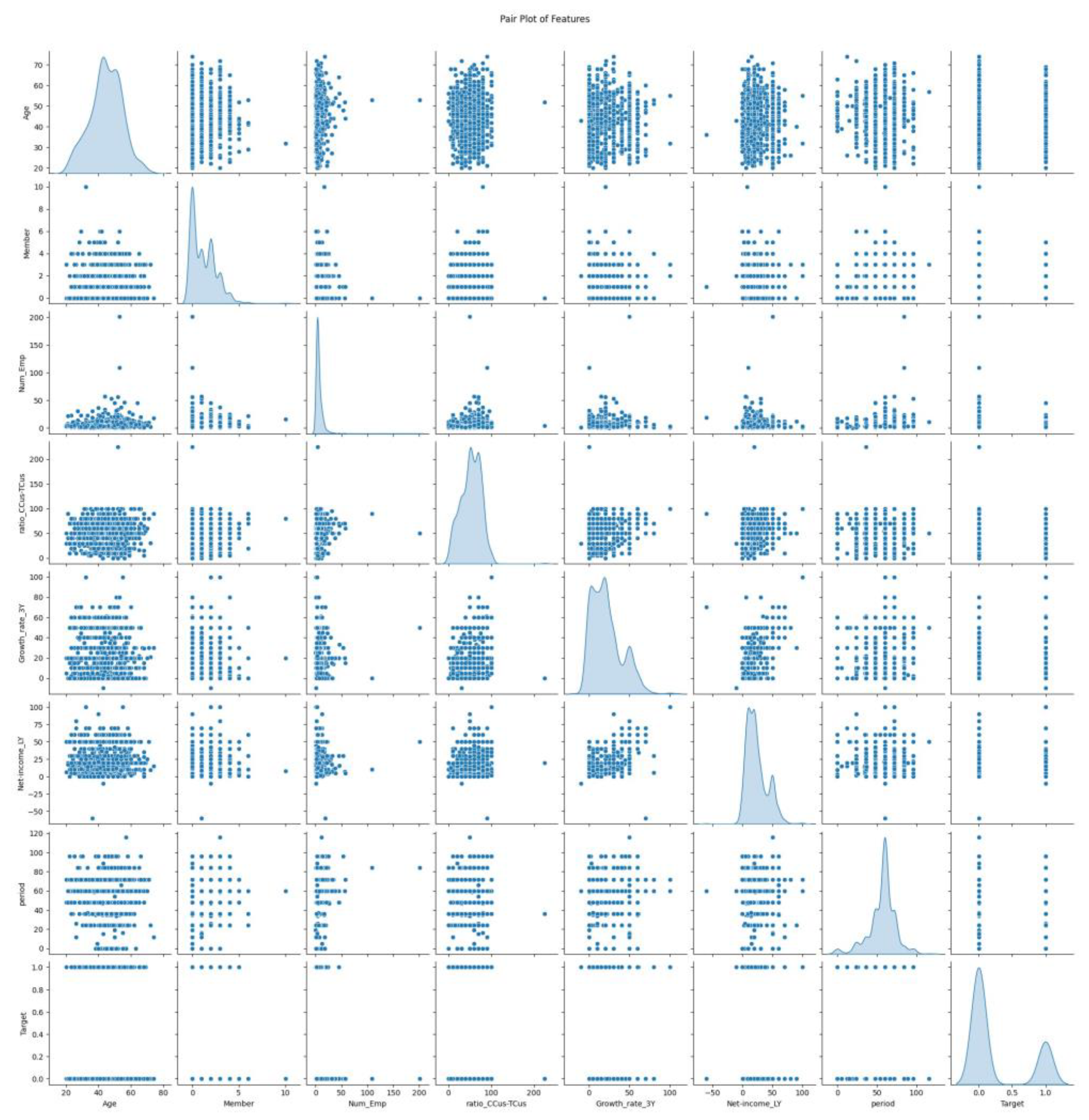
Figure 2.
Workflow of Stacking Model Development, from data preprocessing to final evaluation using stratified cross-validation.
Figure 2.
Workflow of Stacking Model Development, from data preprocessing to final evaluation using stratified cross-validation.
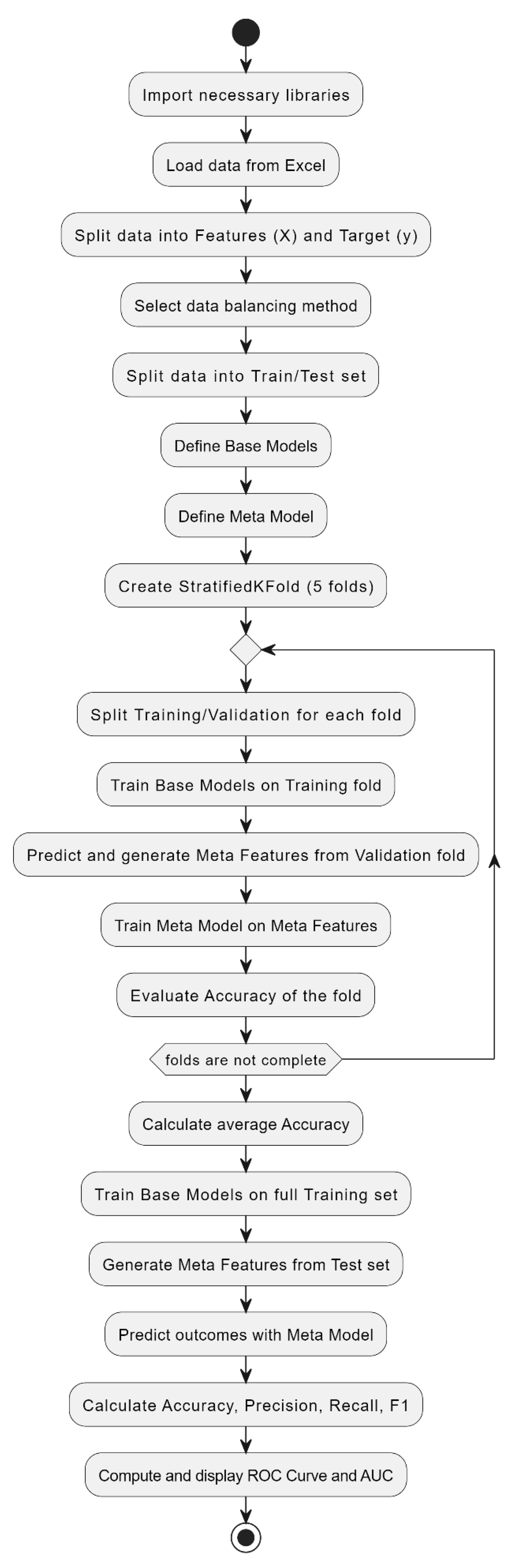
Figure 3.
The problem of class imbalance in the target variable.
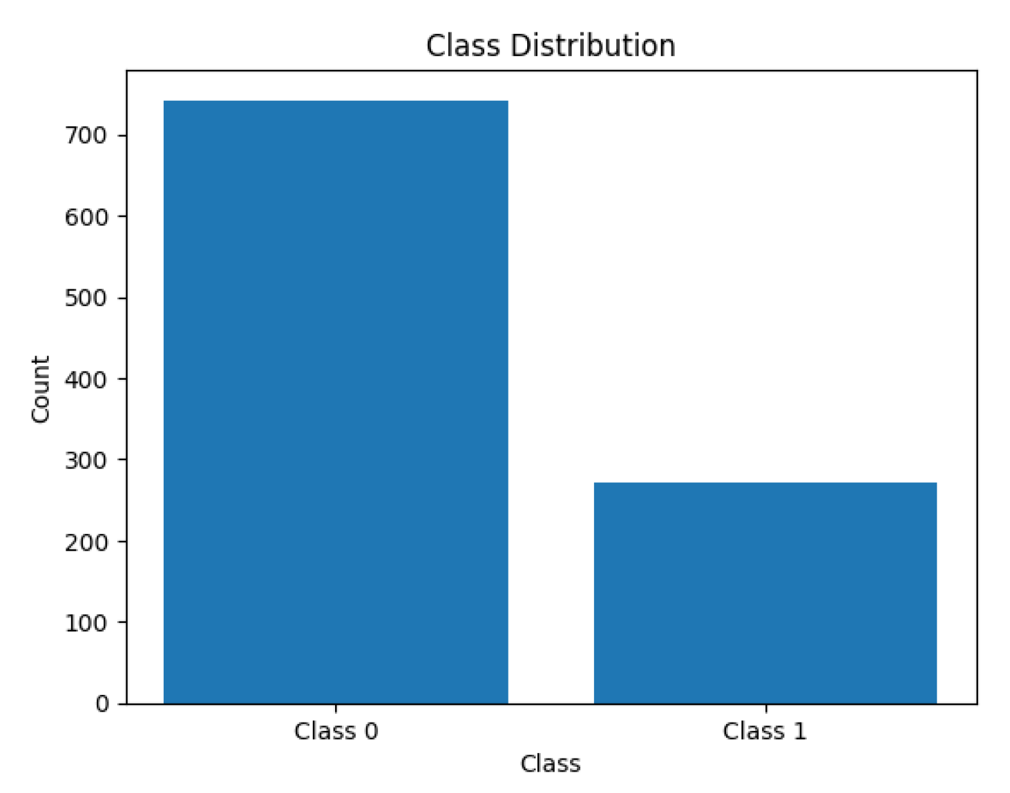
Figure 4.
A comparison of class distributions before and after applying balancing techniques.
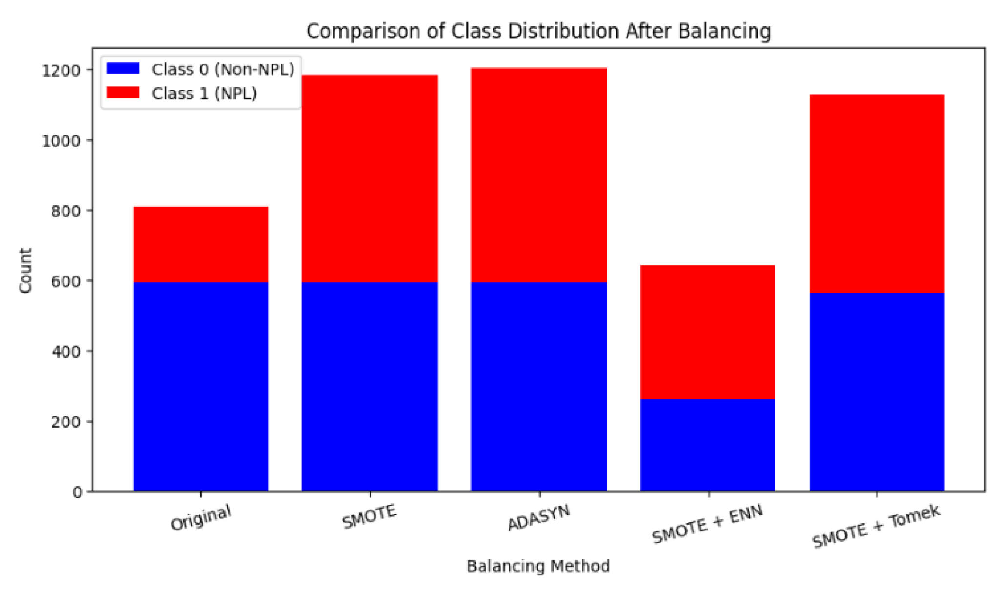
Figure 5.
Performance Comparison Between Full Model vs. Stepwise Model Using SMOTE Technique for Data Balancing.
Figure 5.
Performance Comparison Between Full Model vs. Stepwise Model Using SMOTE Technique for Data Balancing.
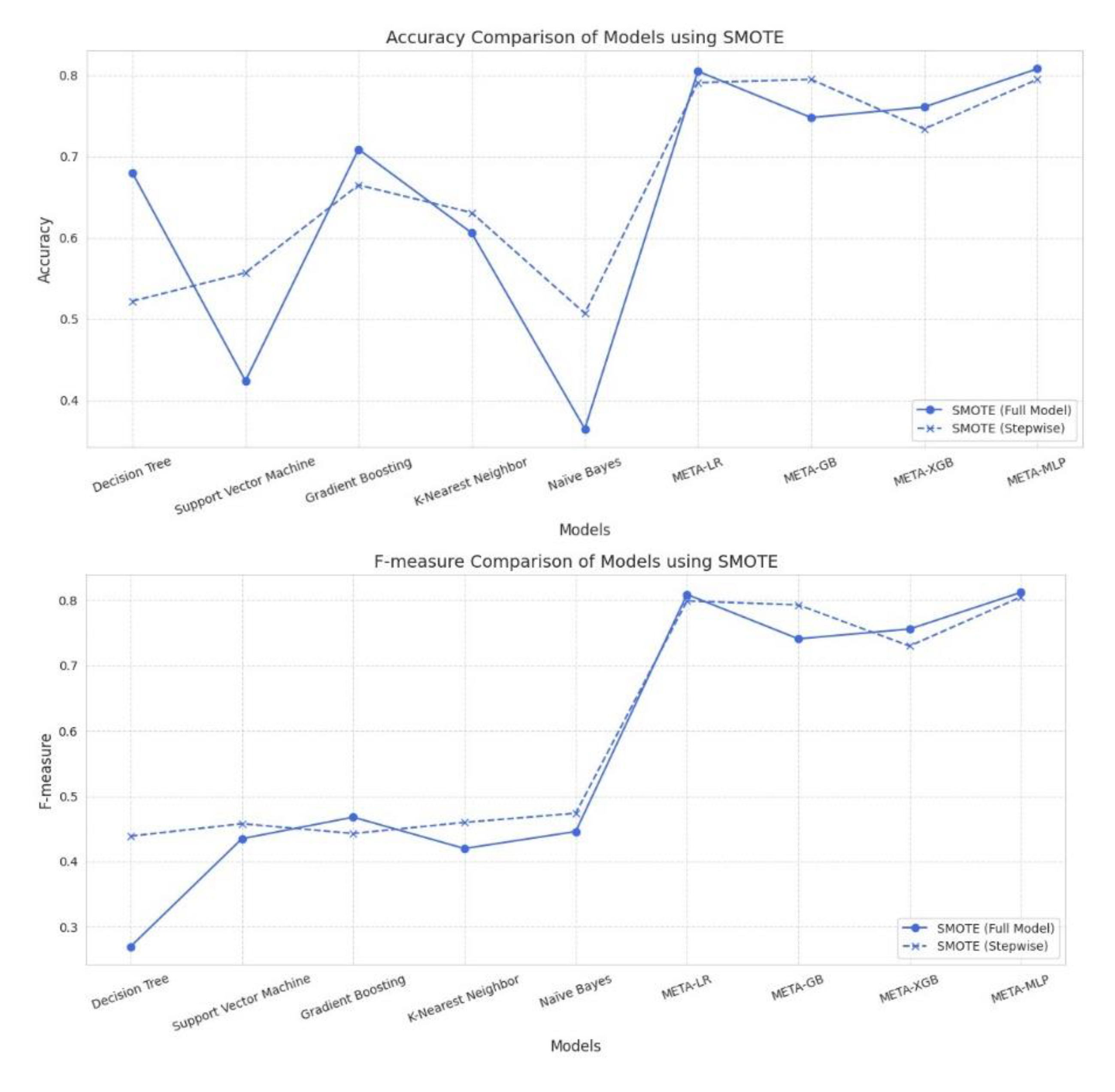
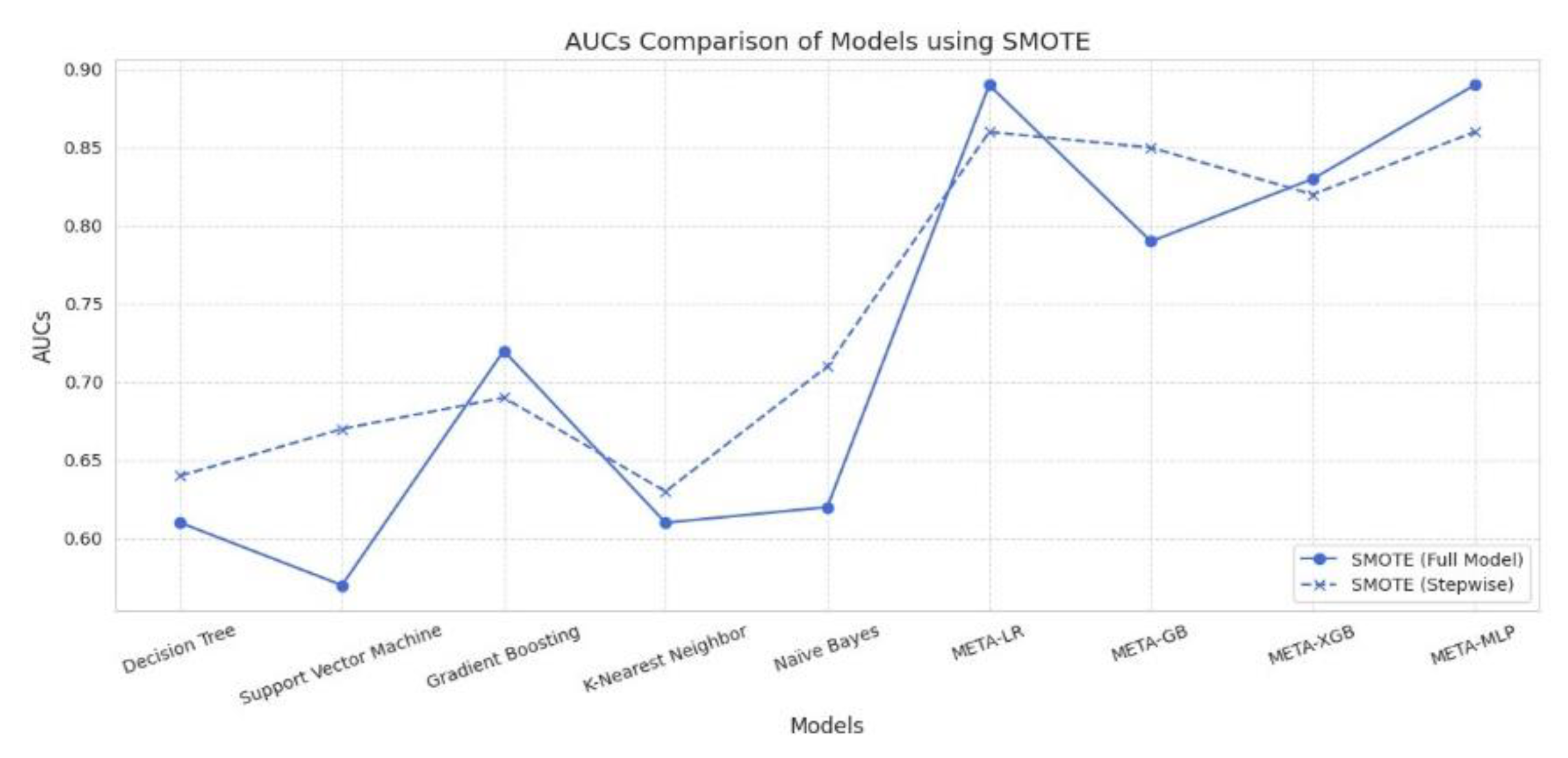
Figure 6.
Performance Comparison Between Full Model vs. Stepwise Model Using ADASYN Technique for Data Balancing.
Figure 6.
Performance Comparison Between Full Model vs. Stepwise Model Using ADASYN Technique for Data Balancing.
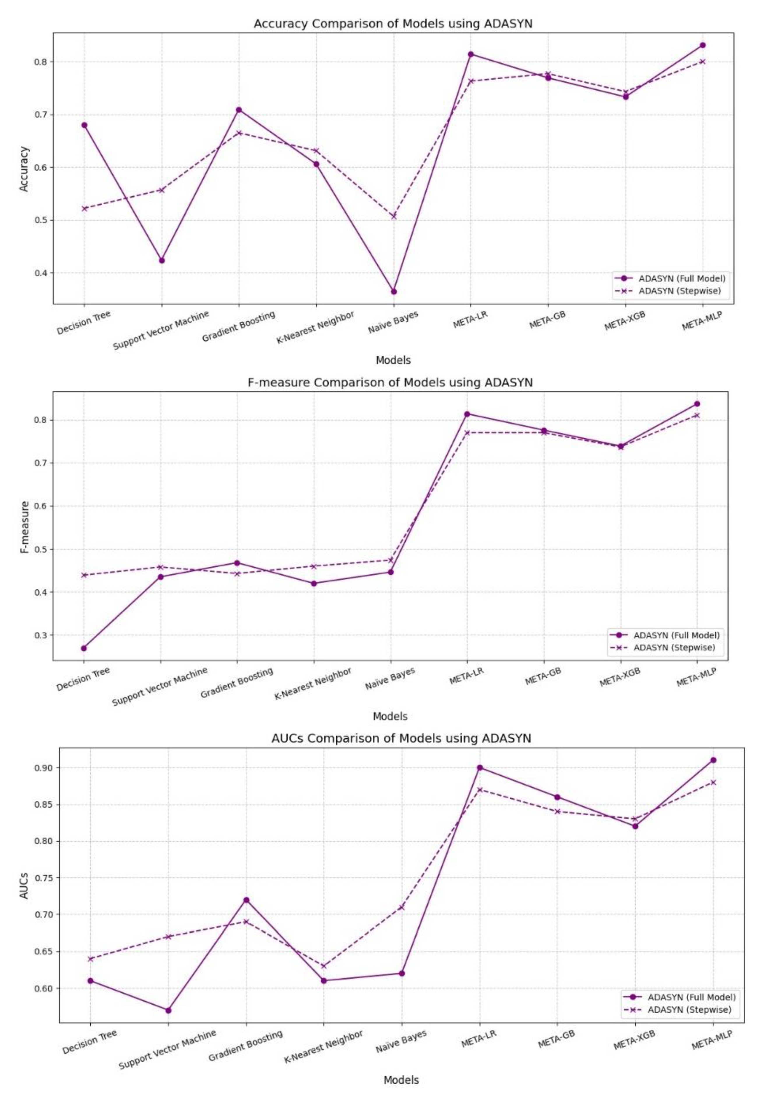
Figure 7.
Performance Comparison Between Full Model vs. Stepwise Model Using SMOTEENN Technique for Data Balancing.
Figure 7.
Performance Comparison Between Full Model vs. Stepwise Model Using SMOTEENN Technique for Data Balancing.
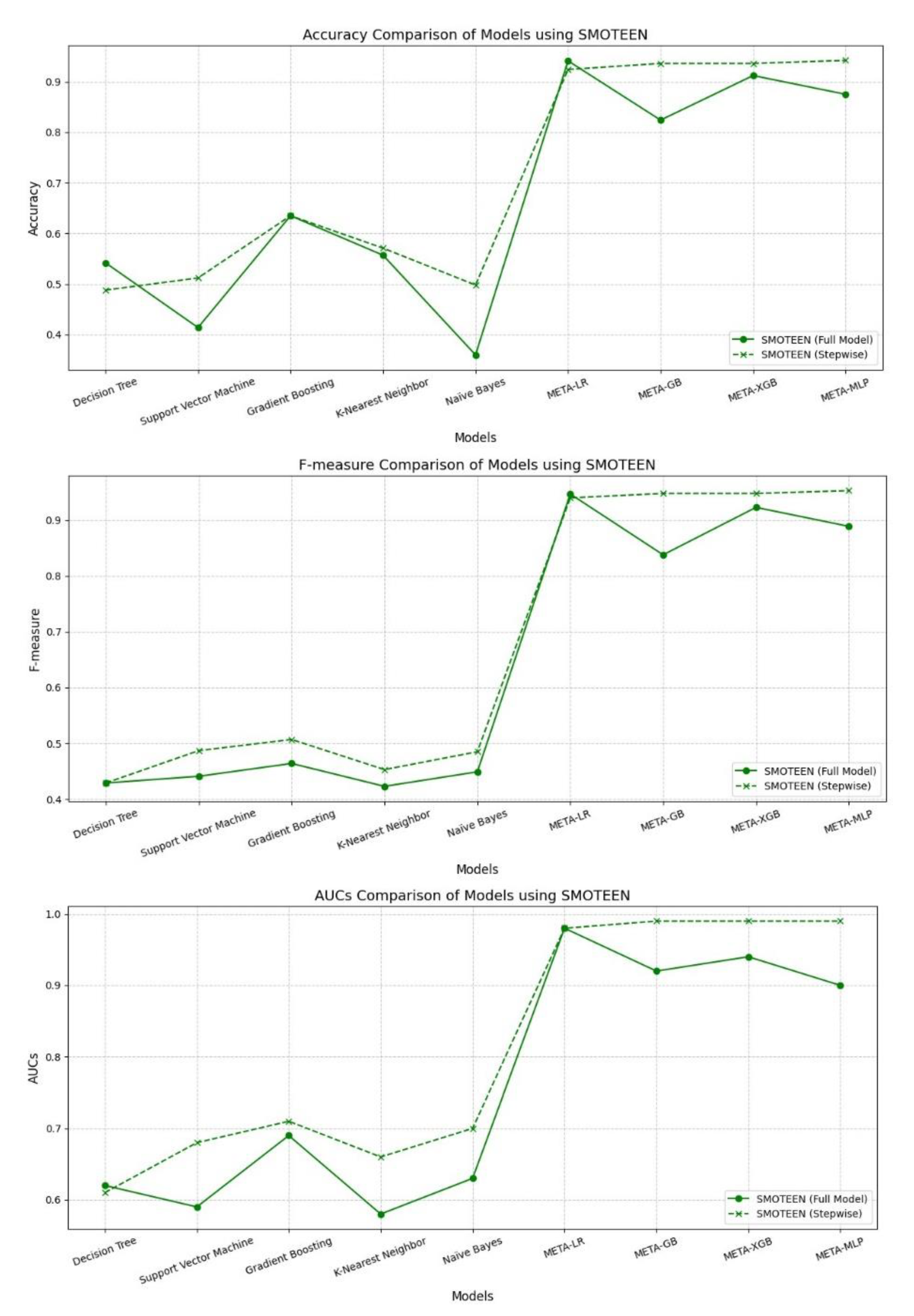
Figure 8.
Performance Comparison Between Full Model vs. Stepwise Model Using SMOTETomek Technique for Data Balancing.
Figure 8.
Performance Comparison Between Full Model vs. Stepwise Model Using SMOTETomek Technique for Data Balancing.
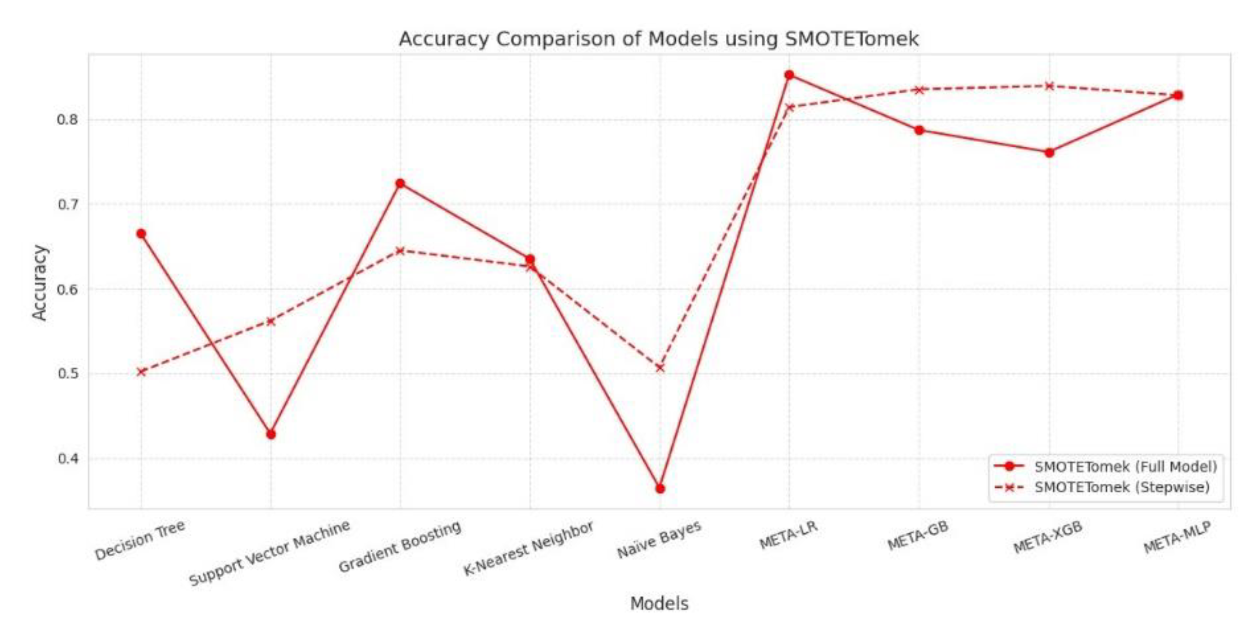
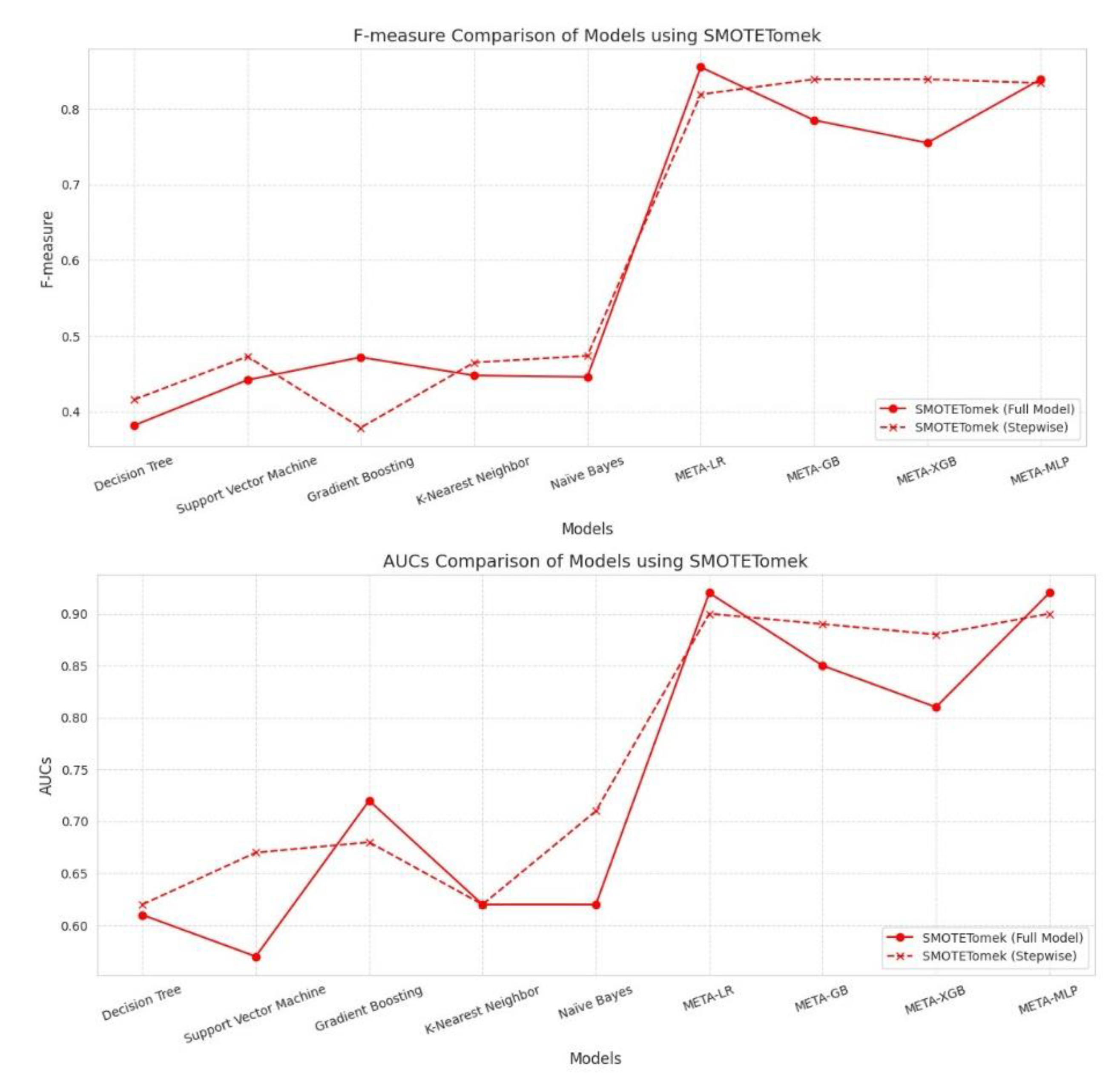
Figure 9.
Performance Comparison Performance Indicators Included Accuracy, Precision, Recall, F1-Score, and AUC-ROC.
Figure 9.
Performance Comparison Performance Indicators Included Accuracy, Precision, Recall, F1-Score, and AUC-ROC.
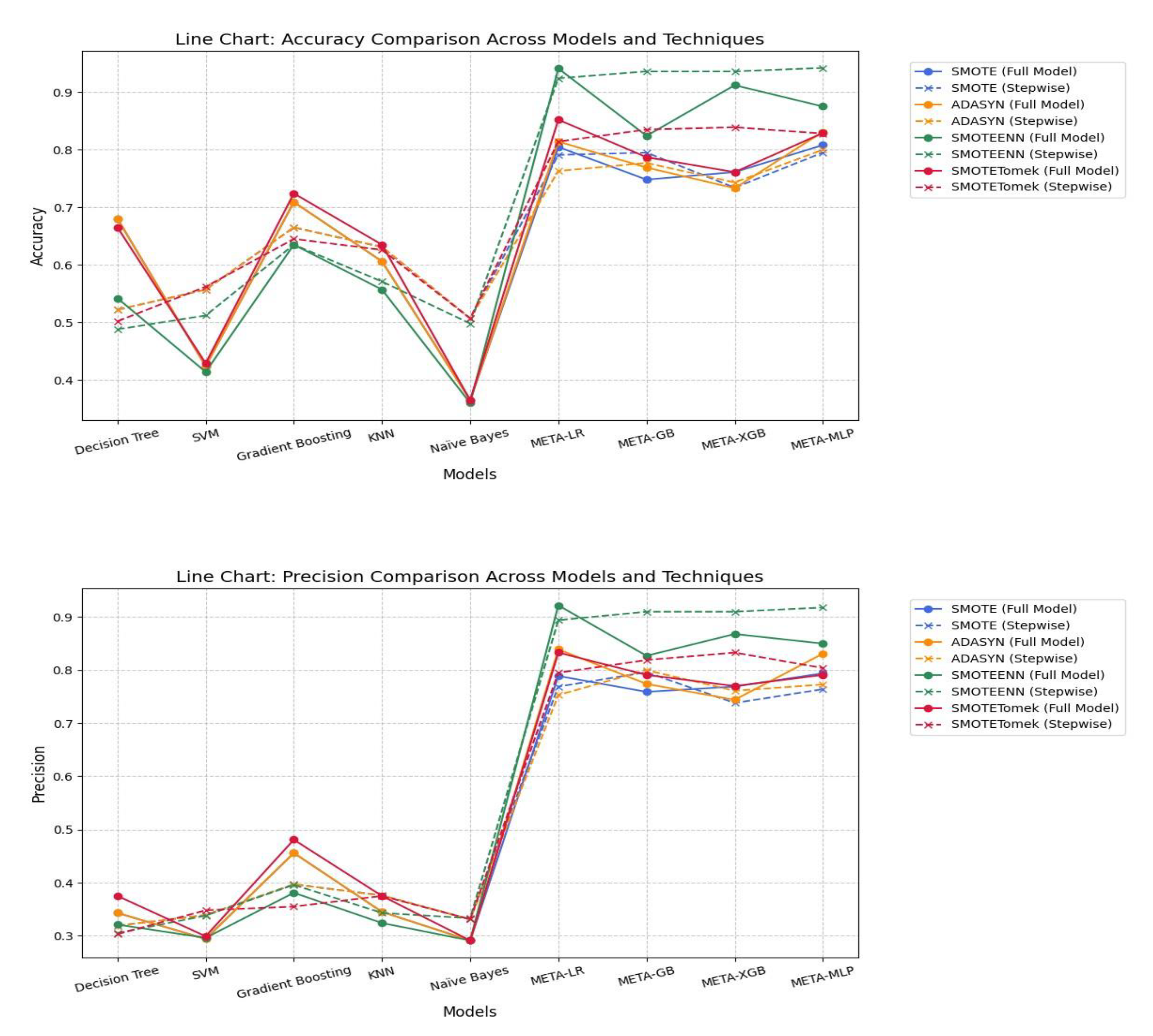
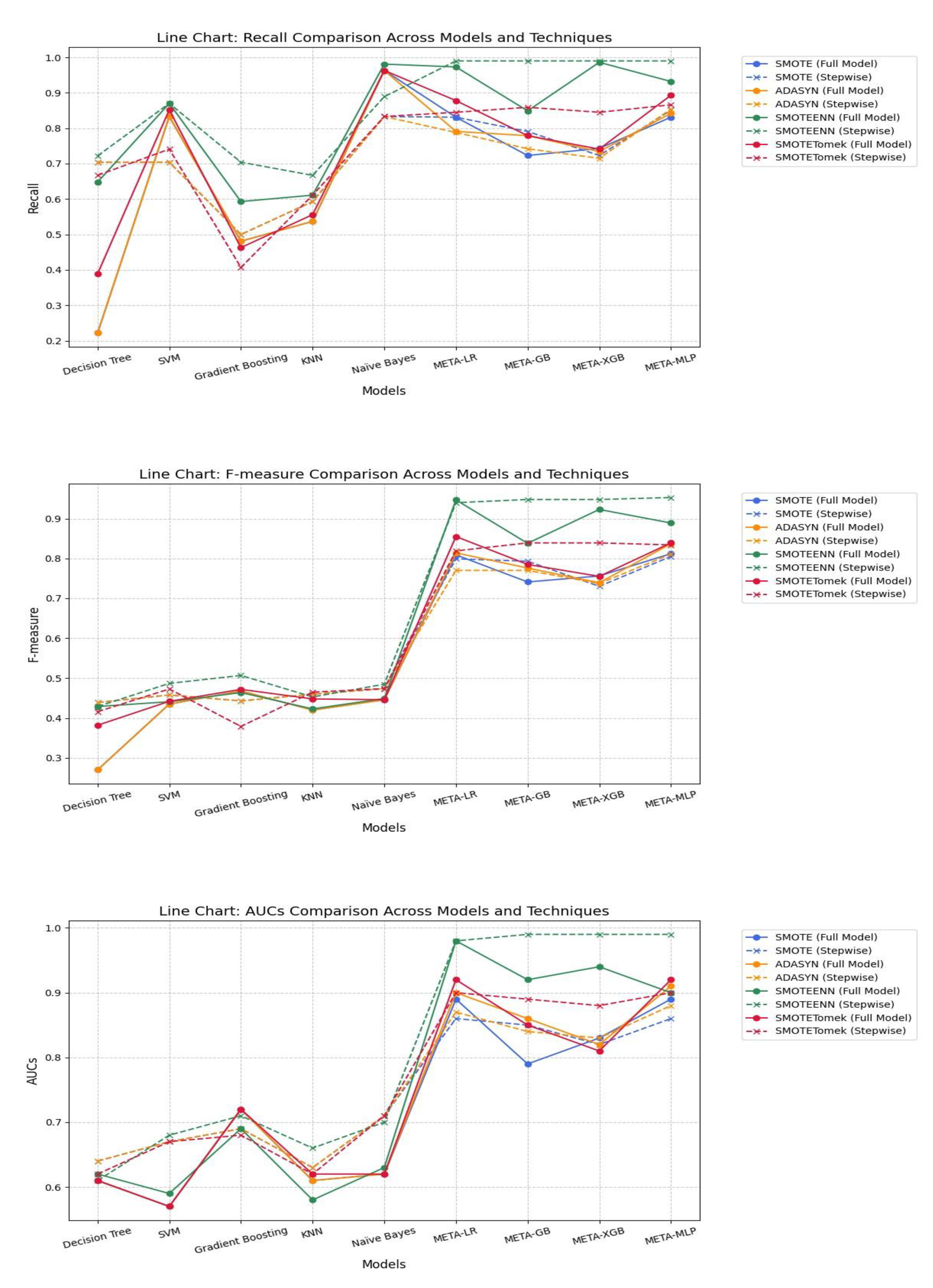
Table 3.
Results of Generalized Linear Regression Model Analysis.
| Variable | Coefficient | S.D. | t | P |
|---|---|---|---|---|
| (Intercept) | 0.7049 | 0.0853 | 8.263 | <0.001*** |
| Age | -0.0035 | 0.0014 | -2.527 | 0.0117* |
| Member | 0.0151 | 0.0104 | 1.45 | 0.1474 |
| Num_Emp | -0.0022 | 0.0015 | -1.491 | 0.1362 |
| ratio_CCus.TCus | 0.0006 | 0.0006 | -2.123 | 0.034* |
| Growth_rate_3Y | -0.0058 | 0.001 | -5.551 | <0.001*** |
| Net.income_LY | 0.0023 | 0.0011 | 2.062 | 0.0394* |
| period | -0.0025 | 0.0008 | -3.126 | 0.0018 |
| *** Statistically Significant at Level. 001 | ||||
| ** Statistically Significant at Level. 01 | ||||
| * Statistically Significant at Level. 05 | ||||
Table 4.
Results of Variance Inflation Factor (VIF) Analysis.
| Variable | Age | Member | Num_Emp | ratio_CCus.TCus | Growth_rate_3Y | Net.income_LY | period |
|---|---|---|---|---|---|---|---|
| VIF | 1.021 | 1.019 | 1.040 | 1.095 | 2.037 | 1.947 | 1.060 |
Table 6.
The number of instances in each class is presented.
| Method | Class 0 | Class 1 | Total |
|---|---|---|---|
| Original | 593 | 272 | 1014 |
| SMOTE | 593 | 593 | 1186 |
| ADASYN | 593 | 611 | 1204 |
| SMOTEENN | 262 | 381 | 643 |
| SMOTETomek | 564 | 564 | 1128 |
Table 7.
Comparison of Model Performance: Baseline vs. META Models Using SMOTE and Full/Stepwise Variables.
Table 7.
Comparison of Model Performance: Baseline vs. META Models Using SMOTE and Full/Stepwise Variables.
| SMOTE | ||||||
|---|---|---|---|---|---|---|
| Model | Accuracy | Precision | Recall | F-measure | AUCs | |
| Decision Tree | Full Model | 0.680 | 0.343 | 0.222 | 0.270 | 0.610 |
| Stepwise | 0.522 | 0.319 | 0.704 | 0.439 | 0.640 | |
| Support Vector Machine | Full Model | 0.424 | 0.294 | 0.833 | 0.435 | 0.570 |
| Stepwise | 0.557 | 0.339 | 0.704 | 0.458 | 0.670 | |
| Gradient Boosting | Full Model | 0.709 | 0.456 | 0.481 | 0.468 | 0.720 |
| Stepwise | 0.665 | 0.397 | 0.500 | 0.443 | 0.690 | |
| K-Nearest Neighbor | Full Model | 0.606 | 0.345 | 0.537 | 0.420 | 0.610 |
| Stepwise | 0.631 | 0.376 | 0.593 | 0.460 | 0.630 | |
| Naïve Bayes | Full Model | 0.365 | 0.291 | 0.963 | 0.446 | 0.620 |
| Stepwise | 0.507 | 0.331 | 0.833 | 0.474 | 0.710 | |
| META-LR | Full Model | 0.805 | 0.789 | 0.831 | 0.809 | 0.890 |
| Stepwise | 0.791 | 0.769 | 0.831 | 0.799 | 0.860 | |
| META-GB | Full Model | 0.748 | 0.759 | 0.723 | 0.741 | 0.790 |
| Stepwise | 0.795 | 0.796 | 0.791 | 0.793 | 0.850 | |
| META-XGB | Full Model | 0.761 | 0.769 | 0.743 | 0.756 | 0.830 |
| Stepwise | 0.734 | 0.738 | 0.723 | 0.730 | 0.820 | |
| META-MLP | Full Model | 0.808 | 0.794 | 0.831 | 0.812 | 0.890 |
| Stepwise | 0.795 | 0.764 | 0.851 | 0.805 | 0.860 | |
Table 8.
Comparison of Model Performance: Baseline vs. META Models Using ADASYN and Full/Stepwise Variables.
Table 8.
Comparison of Model Performance: Baseline vs. META Models Using ADASYN and Full/Stepwise Variables.
| ADASYN | ||||||
|---|---|---|---|---|---|---|
| Model | Accuracy | Precision | Recall | F-measure | AUCs | |
| Decision Tree | Full Model | 0.680 | 0.343 | 0.222 | 0.270 | 0.610 |
| Stepwise | 0.522 | 0.319 | 0.704 | 0.439 | 0.640 | |
| Support Vector Machine | Full Model | 0.424 | 0.294 | 0.833 | 0.435 | 0.570 |
| Stepwise | 0.557 | 0.339 | 0.704 | 0.458 | 0.670 | |
| Gradient Boosting | Full Model | 0.709 | 0.456 | 0.481 | 0.468 | 0.720 |
| Stepwise | 0.665 | 0.397 | 0.500 | 0.443 | 0.690 | |
| K-Nearest Neighbor | Full Model | 0.606 | 0.345 | 0.537 | 0.420 | 0.610 |
| Stepwise | 0.631 | 0.376 | 0.593 | 0.460 | 0.630 | |
| Naïve Bayes | Full Model | 0.365 | 0.291 | 0.963 | 0.446 | 0.620 |
| Stepwise | 0.507 | 0.331 | 0.833 | 0.474 | 0.710 | |
| META-LR | Full Model | 0.814 | 0.839 | 0.791 | 0.814 | 0.900 |
| Stepwise | 0.763 | 0.753 | 0.788 | 0.770 | 0.870 | |
| META-GB | Full Model | 0.769 | 0.774 | 0.779 | 0.776 | 0.860 |
| Stepwise | 0.777 | 0.800 | 0.742 | 0.770 | 0.840 | |
| META-XGB | Full Model | 0.733 | 0.744 | 0.734 | 0.739 | 0.820 |
| Stepwise | 0.743 | 0.761 | 0.715 | 0.737 | 0.830 | |
| META-MLP | Full Model | 0.831 | 0.831 | 0.842 | 0.837 | 0.910 |
| Stepwise | 0.800 | 0.773 | 0.854 | 0.811 | 0.880 | |
Table 9.
Comparison of Model Performance: Baseline vs. META Models Using SMOTEENN and Full/Stepwise Variables.
Table 9.
Comparison of Model Performance: Baseline vs. META Models Using SMOTEENN and Full/Stepwise Variables.
| SMOTEEN | ||||||
|---|---|---|---|---|---|---|
| Model | Accuracy | Precision | Recall | F-measure | AUCs | |
| Decision Tree | Full Model | 0.542 | 0.321 | 0.648 | 0.429 | 0.620 |
| Stepwise | 0.488 | 0.305 | 0.722 | 0.429 | 0.610 | |
| Support Vector Machine | Full Model | 0.414 | 0.296 | 0.870 | 0.441 | 0.590 |
| Stepwise | 0.512 | 0.338 | 0.870 | 0.487 | 0.680 | |
| Gradient Boosting | Full Model | 0.635 | 0.381 | 0.593 | 0.464 | 0.690 |
| Stepwise | 0.635 | 0.396 | 0.704 | 0.507 | 0.710 | |
| K-Nearest Neighbor | Full Model | 0.557 | 0.324 | 0.611 | 0.423 | 0.580 |
| Stepwise | 0.571 | 0.343 | 0.667 | 0.453 | 0.660 | |
| Naïve Bayes | Full Model | 0.360 | 0.291 | 0.981 | 0.449 | 0.630 |
| Stepwise | 0.498 | 0.333 | 0.889 | 0.485 | 0.700 | |
| META-LR | Full Model | 0.941 | 0.922 | 0.973 | 0.947 | 0.980 |
| Stepwise | 0.924 | 0.894 | 0.990 | 0.940 | 0.980 | |
| META-GB | Full Model | 0.824 | 0.827 | 0.849 | 0.838 | 0.920 |
| Stepwise | 0.936 | 0.910 | 0.990 | 0.948 | 0.990 | |
| META-XGB | Full Model | 0.912 | 0.868 | 0.986 | 0.923 | 0.940 |
| Stepwise | 0.936 | 0.910 | 0.990 | 0.948 | 0.990 | |
| META-MLP | Full Model | 0.875 | 0.850 | 0.932 | 0.889 | 0.900 |
| Stepwise | 0.942 | 0.918 | 0.990 | 0.953 | 0.990 | |
Table 10.
Comparison of Model Performance: Baseline vs. META Models Using SMOTETomek and Full/Stepwise Variables.
Table 10.
Comparison of Model Performance: Baseline vs. META Models Using SMOTETomek and Full/Stepwise Variables.
| SMOTETomek | ||||||
|---|---|---|---|---|---|---|
| Model | Accuracy | Precision | Recall | F-measure | AUCs | |
| Decision Tree | Full Model | 0.665 | 0.375 | 0.389 | 0.382 | 0.610 |
| Stepwise | 0.502 | 0.303 | 0.667 | 0.416 | 0.620 | |
| Support Vector Machine | Full Model | 0.429 | 0.299 | 0.852 | 0.442 | 0.570 |
| Stepwise | 0.562 | 0.348 | 0.741 | 0.473 | 0.670 | |
| Gradient Boosting | Full Model | 0.724 | 0.481 | 0.463 | 0.472 | 0.720 |
| Stepwise | 0.645 | 0.355 | 0.407 | 0.379 | 0.680 | |
| K-Nearest Neighbor | Full Model | 0.635 | 0.375 | 0.556 | 0.448 | 0.620 |
| Stepwise | 0.626 | 0.375 | 0.611 | 0.465 | 0.620 | |
| Naïve Bayes | Full Model | 0.365 | 0.291 | 0.963 | 0.446 | 0.620 |
| Stepwise | 0.507 | 0.331 | 0.833 | 0.474 | 0.710 | |
| META-LR | Full Model | 0.852 | 0.833 | 0.878 | 0.855 | 0.920 |
| Stepwise | 0.814 | 0.795 | 0.845 | 0.819 | 0.900 | |
| META-GB | Full Model | 0.787 | 0.791 | 0.779 | 0.785 | 0.850 |
| Stepwise | 0.835 | 0.819 | 0.859 | 0.839 | 0.890 | |
| META-XGB | Full Model | 0.761 | 0.770 | 0.741 | 0.755 | 0.810 |
| Stepwise | 0.839 | 0.833 | 0.845 | 0.839 | 0.880 | |
| META-MLP | Full Model | 0.829 | 0.791 | 0.893 | 0.839 | 0.920 |
| Stepwise | 0.828 | 0.804 | 0.866 | 0.834 | 0.900 | |
Table 11.
Performance comparison of baseline approach and all models under SMOTEENN and Stepwise Feature Selection.
Table 11.
Performance comparison of baseline approach and all models under SMOTEENN and Stepwise Feature Selection.
| Model | Accuracy | Precision | Recall | F-measure | AUCs |
|---|---|---|---|---|---|
| Baseline Approach (Mode) | 0.734 | - | - | - | - |
| Decision Tree | 0.488 | 0.305 | 0.722 | 0.429 | 0.610 |
| Support Vector Machine | 0.512 | 0.338 | 0.870 | 0.487 | 0.680 |
| Gradient Boosting | 0.635 | 0.396 | 0.704 | 0.507 | 0.710 |
| K-Nearest Neighbor | 0.571 | 0.343 | 0.667 | 0.453 | 0.660 |
| Naïve Bayes | 0.498 | 0.333 | 0.889 | 0.485 | 0.700 |
| META-LR | 0.924 | 0.894 | 0.990 | 0.940 | 0.980 |
| META-GB | 0.936 | 0.910 | 0.990 | 0.948 | 0.990 |
| META-XGB | 0.936 | 0.910 | 0.990 | 0.948 | 0.990 |
| META-MLP | 0.942 | 0.918 | 0.990 | 0.953 | 0.990 |
Disclaimer/Publisher’s Note: The statements, opinions and data contained in all publications are solely those of the individual author(s) and contributor(s) and not of MDPI and/or the editor(s). MDPI and/or the editor(s) disclaim responsibility for any injury to people or property resulting from any ideas, methods, instructions or products referred to in the content. |
© 2025 by the authors. Licensee MDPI, Basel, Switzerland. This article is an open access article distributed under the terms and conditions of the Creative Commons Attribution (CC BY) license (http://creativecommons.org/licenses/by/4.0/).
Copyright: This open access article is published under a Creative Commons CC BY 4.0 license, which permit the free download, distribution, and reuse, provided that the author and preprint are cited in any reuse.


