
Submitted:
28 July 2025
Posted:
06 August 2025
You are already at the latest version
Abstract
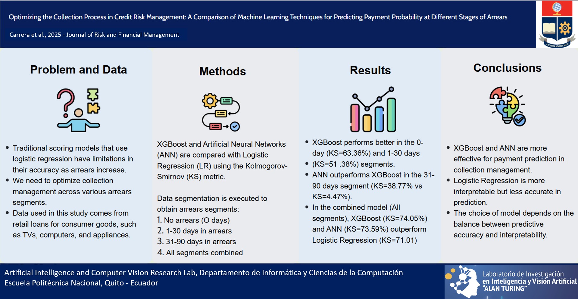
In credit risk, scoring models based on logistic regression have been developed to optimize the default risk assessment. However, these models require complex feature engineering and their accuracy worsens as the arrear progresses.
This study proposes the use of machine learning techniques (XGBoost and Artificial Neural Networks) to generate scores in different arrear segments (No Arrears Segment, Segment 1-30 days of arrears, Segment 31-90 days of arrears, and All Segments). The Kolmogorov-Smirnov (KS) metric is used to assess the efficiency and predictive power of the models. To ensure the accuracy and reliability of the models, a five-step methodology is employed. It starts with the formulation of the problem, followed by the selection of a data sample and definition of the target variable, then a descriptive analysis of the data is performed to facilitate the data cleaning. Subsequently, the models are trained and tested, and finally, the results are analyzed and the models obtained are interpreted. The results show that both XGBoost and Artificial Neural Networks models outperform logistic regression in most of the arrears segments. In the No Arrears Segment, XGBoost model is the best with KS=63.36%. In the Segment 1-30, XGBoost is also the best with KS=51.38%. In the Segment 31-90, Artificial Neural Networks model is the best with KS=38.77%. Finally, with all segments of arrears, XGBoost model
again is the best with KS=74.05%.
Keywords:
XGboost
; artificial neural networks
; logistic regression
; credit scoring
; credit risk management
1. Introduction
1.1. Problem Statement
In mass credit management, scoring models have proven to be the most valuable tool for the past two decades. By analyzing historical data, these models provide predictions of future behavior, which help control portfolios with greater accuracy and less uncertainty. A scoring model considers numerous variables simultaneously, which helps to establish a pattern and group members together based on their likelihood of experiencing an event. These models work best when dealing with large volumes of data with relatively homogeneous values. It is important to note that scoring models are designed to identify patterns and groupings, rather than to provide precise predictions for individual cases. (see Figure 2)
Due to its ease of interpretation, logistic regression is the favorite in this kind of problems. However, with the increase in available information, the growth over time of debtors, and more lenders, obtaining a score with a high predictive capacity becomes a much more complex task.
1.2. Scoring Models for Credit Collection
Effective collections management is a critical aspect of managing large credit portfolios. It affects not only customer interactions, but also collections operations. Without access to agile and effective tools, negative reactions from customers to their payment obligations are likely to occur. In the credit world, it is commonly understood that as the age of arrears increases, the chances of recovering funds decrease. It is therefore imperative to develop effective strategies to prevent this situation from occurring.
Typically, collections management relies on portfolio segmentation and customer contact channels to determine the appropriate actions based on the number of days in arrears, the type of product and the likelihood of payment. This approach may involve a variety of methods such as phone calls, field visits, text messages, emails or letters to encourage customers to meet their obligations and ensure a positive outcome. (see Figure 1)
When implementing scoring models for collections, it is crucial to consider the number of days that have passed since the loan was due, to determine whether it is still recoverable. Hence, it is recommended to segment the portfolio into 30 or 15-day arrears ranges, based on the loan disbursement terms. Therefore, the following arrears segments are possible:
- 0 - No Arrears segment
- 1 - 30 segment
- 31 - 60 segment
- 61 - 90 segment
- 91 - 120 segment
- More than 120 segment
Where More than 120 is considered as a loss segment.
When arrears increase, it is crucial to differentiate between each segment and design a scoring model to distinguish reliable payers from those who default on payments. It is essential to keep in mind that as arrears increase, the number of individuals decreases, which may impact the model’s ability to predict. However, thankfully, we can measure the scoring model’s ability to discriminate using the Kolmogorov-Smirnoff (KS) metric.
1.3. Literature Review
This section reviews some efforts to predict the probability of client default to make informed lending decisions. We explore various modeling techniques, including logistic regression, XGBoost, and artificial neural networks, and evaluate their performance using the Kolmogorov-Smirnov (KS) statistic.
1.3.1. Credit Scoring with Logistic Regression
Logistic regression is a frequently utilized statistical method in the credit rating industry because of its capability to model the likelihood of a binary event, such as a credit default [23]. This model is renowned for its interpretability and predictive accuracy. Recent research has shown that logistic regression has achieved remarkably high accuracy in forecasting credit risk, reaching up to 99% in certain instances [22].
1.3.2. Credit Scoring with XGBoost
XGBoost, a decision tree-based machine learning algorithm, is widely acclaimed for its exceptional performance in classification and regression tasks. This model excels at uncovering intricate patterns in data and has demonstrated successful applications in credit risk prediction [4]. However, there have been instances where XGBoost has underestimated credit risk, indicating the necessity for further refinements and validations [27].
1.3.3. Credit Scoring with Artificial Neural Networks
Artificial neural networks are adept at capturing non-linear and complex relationships between variables, making them well-suited for predicting credit defaults [25] [8]. In comparative studies, neural networks have demonstrated performance comparable to logistic regression, achieving an accuracy of 71% in training and 72% in testing [25].
1.3.4. Performance Evaluation
The Kolmogorov-Smirnov (KS) statistic is a metric utilized to evaluate the predictive performance of scoring models. It measures the difference between the cumulative distributions of good and bad payers’ scores, indicating the degree of distinction between the two sets of scores. Recent studies have incorporated KS alongside other metrics like the area under the ROC curve and the GINI test to evaluate and compare the effectiveness of various models [23] [20].
1.3.5. Comparison of Models
In comparing models for credit risk prediction, logistic regression, neural networks, and XGBoost have all been identified as suitable techniques. Each method has its own strengths and weaknesses. Logistic regression is highly interpretable and exhibits high accuracy in predicting credit extension [23] [22]. XGBoost, on the other hand, delivers high performance and can handle large amounts of data, although it may require additional adjustments to prevent underestimating risk [6]. While neural networks are complex, they can capture non-linear relationships and have demonstrated performance comparable to logistic regression [25] [8].
In sum, selecting the most suitable modeling technique for credit scoring and collections depends on various factors such as interpretability, data volume, and predictive capability. Viable techniques include logistic regression, XGBoost, and artificial neural networks, each with their distinct advantages and limitations. Evaluating performance using metrics like the Kolmogorov-Smirnov statistic is essential for assessing the efficacy of each model in predicting credit risk.
This study, unlike previous studies, explores the effectiveness of conventional logistic regression compared to two machine learning techniques, Extreme Gradient Boosting (XGBoost) and artificial neural networks (ANNs), in predicting the ability to pay at different delinquency levels of a large retail loan portfolio. Using the KS metric, the performance of each model at each arrear segment is measured.
Figure 2.
Credit Scoring Scheme.
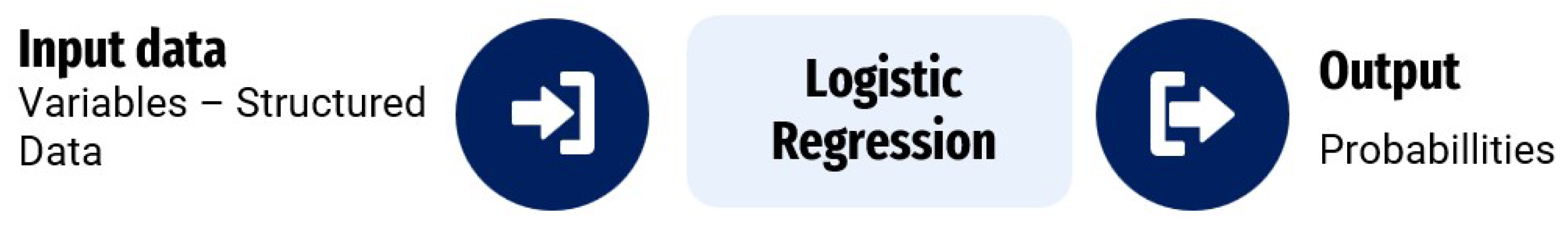
Currently, efforts are focused on feature engineering to find better predictors to maximize the discrimination of logistic regression-based models. The objective is often to estimate the probability that a customer will pay off his debt, determine his risk level in case of loan approval, or assess the cost-effectiveness of offering several products to the same person.
In this paper, we focus on maximizing the predictive power of the model by testing different supervised learning techniques in the recovery phase of loans at different arrears segments.
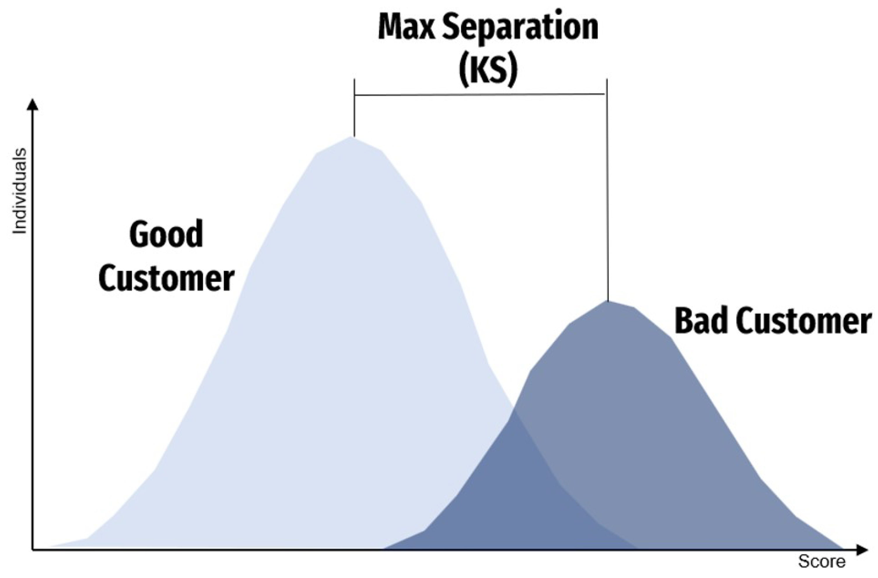
Figure 3.
Representation of the separation or divergence of two probability distributions.
2. Methodology
2.0.1. Kolmogorov-Smirnov Tests
The K-S test, or Kolmogorov-Smirnov test, is a non-parametric method utilized to assess the similarity of two distinct continuous distributions. It evaluates the hypothesis of whether or not they are identical. The KS statistic is computed by employing the cumulative empirical distribution function [1].
Consider two samples and of size and respectively, with cumulative distribution functions and of a continuous random variable X. The KS test is used to test hypotheses:
Based on the use of the empirical cumulative distribution function (1), the KS statistic is used to test the null hypothesis . Its value is obtained using the following expression:
The notation represents the empirical accumulation function of and represents the empirical distribution function of . If the KS statistic is greater than the critical value for a given significance level , we reject the null hypothesis . In [18], you can find a table of critical values for different sample sizes.
Then, the KS statistic is a measure of divergence between the distributions of two variables. It is the maximum distance between and , and its value ranges between 0 and 1. Values close to 0 indicate that the distributions of and are identical, while values close to 1 indicate that the distributions of and differ. Therefore, the KS statistic is useful for distinguishing the differences between two distributions.
In our current project, we aim to determine the classification technique that achieves the highest KS value. We will compare the results of logistic regression, Extreme Gradient Boosting, and Artificial Neural Networks. The predicted score values for individuals who are categorized as good customers with 0 will be represented by , while the predicted score values for individuals who are categorized as bad customers with 1 will be represented by .
2.1. Data Sample Selection
When building a scoring model, it is important to collect as much information as possible that has been generated during the life of the loan. At the collection stage, it is especially essential to have data on payment behavior at the lending institution, information on the social and demographic profile of the customer, and data on collection performance. Sometimes it may also be useful to include information on payment behaviour at other financial institutions.
For our study, we have focused on loans granted directly to consumers in the retail sector, which includes credit for items such as televisions, computers, technology, household appliances, and other consumer goods. To explain the information needed to develop the scoring models, consider Figure 4. The period of time prior to the observation point is called the ‘behavioural window’, which cannot be longer than 36 months according to the provision of the superintendence of banks and insurance of Ecuador.
Figure 4.
Historic Data Selection.
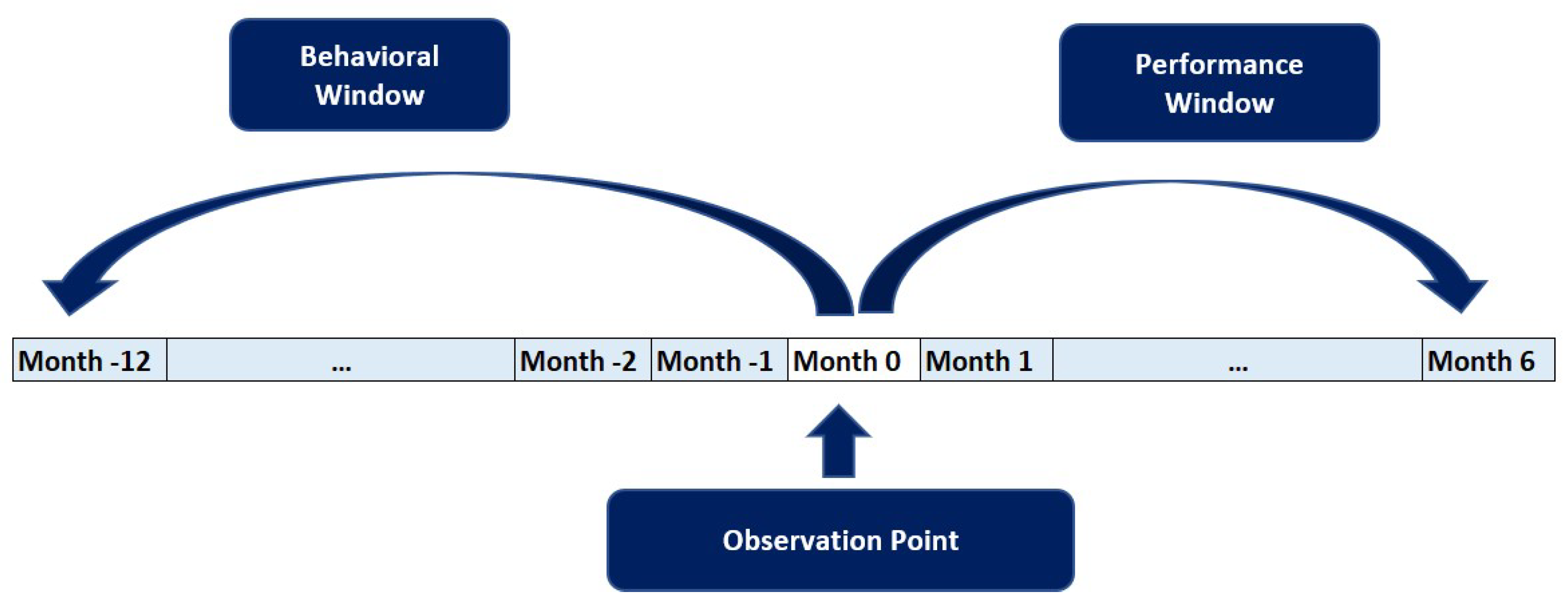
Normally, a 36-month history is used when scoring models are created. However, during the collection phase, using such a long history can be counterproductive. This is because the collection stage is much more dynamic and unpredictable, and mistakes can be made by considering ancient payment behavior that may not reflect the current situation. As a result, it can be difficult to predict your next payment, so we use 12 months of history. During this period, variables related to the individual’s credit history are generated, such as payment and borrowing habits, maximum and average delinquency, open transactions, telephone transactions, actual telephone contacts, card payments, consumption amounts, etc. At the observation point, socio-demographic variables such as age, marital status, province, region, etc. are generated.
After the observation point, we evaluate an individual’s payment behavior during a period called the "performance window". This window provides crucial information that helps us define good and bad individuals (dependent variable Y). Since payments are made monthly, we use a one-month window to determine whether a payment has been made or not. After that, we evaluate the individual’s payment behavior over a period of 6 months.
2.2. Dependent Variable Setting
The dependent variable Y is binary, with a value of 1 assigned to individuals marked as "Good Customer" and 0 assigned to those identified as "Bad Customer". We will be using two different definitions to evaluate performance. The first is based on payment events within a one-month performance window, while the second is based on monthly payment behavior within a 6-month performance window.
Definition 2.1.
Payment Event
Definition 2.2.
Monthly Payment Behavior
With , the aim is to have as few clients as possible switch to higher arrears ranks. This definition will be used in each arrears range to discriminate between good and bad clients. On the other hand, with , the aim is to control the deterioration of the portfolio in the medium term, to avoid excessive losses.
3. Train and Test Models
A scoring model is created by identifying patterns within the predictor variables, which can be used to classify individuals into good and bad categories based on the event to be predicted. In machine learning, this model is developed through supervised learning, where the model is trained with data that is different from the data used in the training phase.
It is crucial to have a diverse dataset during the training phase to ensure that the model is trained on a wide range of information. In order to achieve this, the data needs to be randomly split into three datasets. The first dataset, comprising 60% of the data, is used for training. The second dataset, containing 25% of the data, is used for testing. Finally, the remaining 15% of the data is used for validation.
Table 1 the distribution of the training, testing, and validation samples. Meanwhile, Table 2 indicates the distribution of customers classified as good and bad, for and .
3.1. Logistic Regression Training
Logistic regression is a widely used technique for predicting a categorical variable using a set of explanatory variables. It is a parametric method that is formulated as follows.
Consider N quantitative variables . For each combination of these variables, the response variable Y follows a Bernoulli distribution [21].
We are interested in modelling the conditional expectation.
The multiple logistic regression model for Y in terms of the values of the variables X, can be modelled as:
with and
In matrix terms it would be
with and
Finally, a linear model for the logit transformation is obtained.
3.1.1. Unbalanced Problem
In some cases where we use logit, probit or linear probability models, the number of observations in one group is much smaller than in the other. For instance, in lending, the number of bad clients is expected to be much smaller than the number of good clients because if both were equal, the financial institution would face bankruptcy. Therefore, to reach accurate predictions, we need either a large dataset or a balanced sample containing equal proportions of both groups. In this case, we would consider all bad customers and sample the good customers to achieve a 50/50 ratio.
The question arises as to how we can analyze data in such cases. We suggest using a weighted logit (or probit or linear probability) model, similar to weighted least squares. If the logit model is used for estimating the coefficients of the explanatory variables, the different sample sizes for the two groups do not affect the coefficients [17].
Let and be the sample proportions of the two groups, with . Since is the probability that an observation belonging to the first group is selected, and is the probability that an observation belonging to the second group is selected, when the samples are disproportionate the logistic function is shifted as follows:
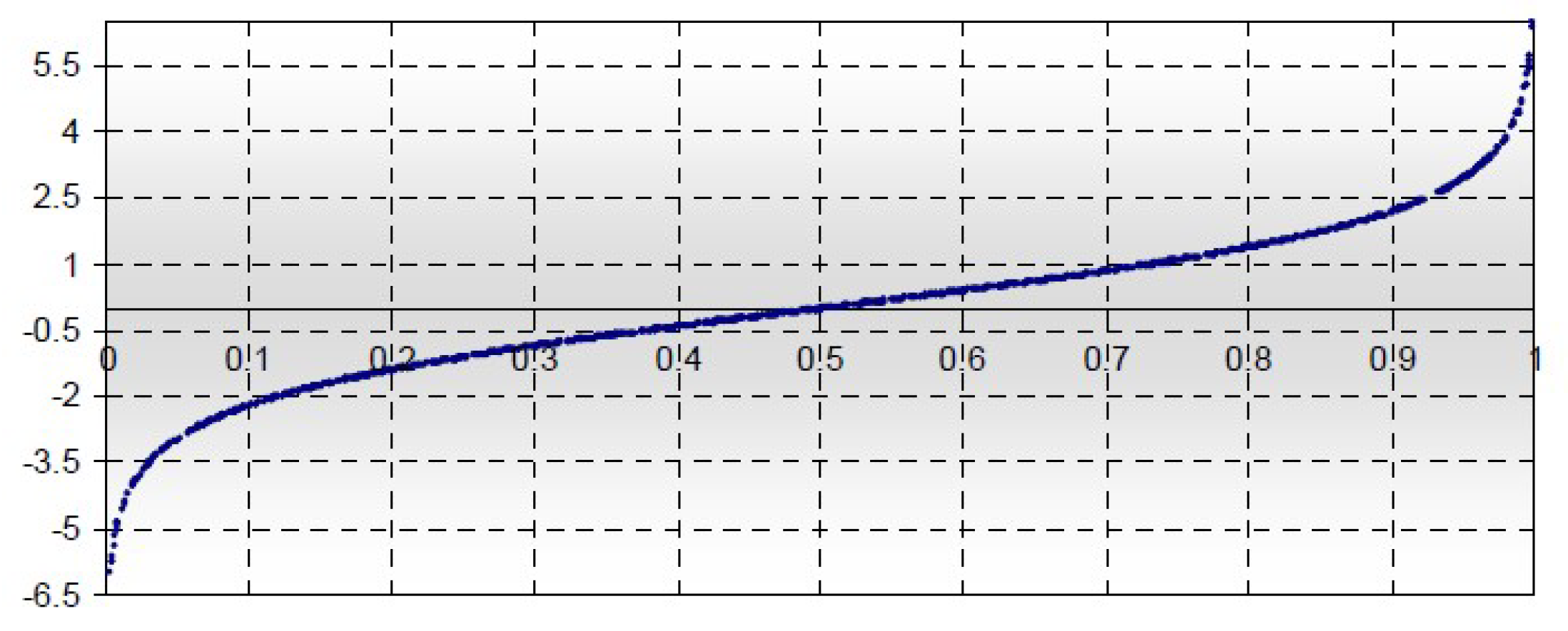
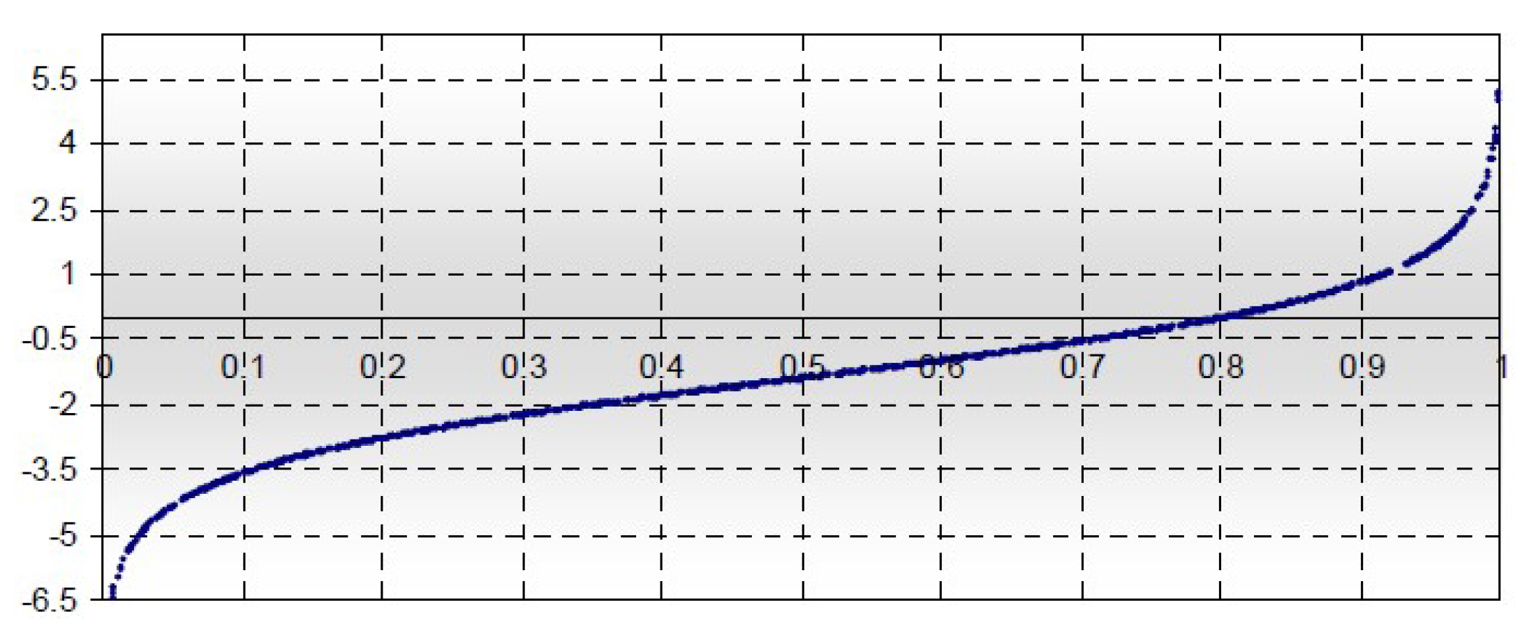
When the logistic function cuts on the x-axis, at the value 0.5, as seen in Figure 5. Now, if and the curve shifts and cuts on the x-axis at 0.8, as seen in Figure 6.
Figure 5.
Logit Function.
Therefore, the disproportionality of the samples only affects the constant term of the model and one has that
where , .
[13]
Figure 6.
Shifted Logit Function.
3.2. Extreme Gradient Boosting Training
XGBoost (Extreme Gradient Boosting) is a machine-learning algorithm introduced by Chen and Guestrin in 2016. It uses the concept of tree gradient boosting to improve its performance and speed. XGBoost was designed to reduce overfitting by introducing regularization parameters. Gradient boosting trees use regression trees in a sequential learning process as weak learners. These regression trees are similar to decision trees, but they assign a continuous score to each leaf that is then summarized to provide the final prediction [5].
Several hyperparameters are relevant when it comes to training a model. Some of them include the learning rate, column subsampling, and regularisation rate. Additionally, subsampling (which involves bootstrapping the training sample), the maximum depth of the trees, the minimum weights on the children’s scores to split, and the number of estimators (trees) are also commonly used to address the bias-variance-compensation. While higher values for the number of estimators, regularisation, and weights on secondary grades are associated with reduced overfitting, learning rate, maximum depth, subsampling, and column subsampling should have lower values to achieve reduced overfitting. However, setting extreme values for any of these hyperparameters can lead to model misfits.
3.2.1. Hyperparameter Selected and Tuning
Hyperparameters are settings or configurations of the methods (models), which are freely selectable within a certain range and influence model performance (quality).
Grid search in XGBoost is an optimization technique that seeks to find the set of hyperparameters that yields the most accurate predictive model. It operates by defining a grid of hyperparameter values and evaluating the model’s performance for each combination of these values. This process is facilitated by the use of cross-validation, typically k-fold cross-validation, to assess the performance of the model on different subsets of the training data, thereby ensuring that the model’s performance is robust and not overly dependent on the particularities of one set of training data. [2]
The hyperparameters commonly tuned in XGBoost through grid search include , , , , , and (). The grid search process evaluates the model for each combination of hyperparameters in the grid, which can be computationally intensive but is necessary for identifying the optimal parameters that minimize overfitting and maximize predictive performance.
3.2.2. XGBoost Hyperparameter Nrounds
The parameter specifies the number of boosting steps and takes values between where only integer values are valid. Since a tree is created in each individual boosting step, also controls the number of trees that are integrated into the ensemble as a whole. Its practical meaning can be described as follows: larger values of mean a more complex and possibly more precise model, but also cause a longer running time.
3.2.3. XGBoost Hyperparameter Eta
The parameter is a learning rate and is also called "shrinkage" parameter and takes values between . It controls the lowering of the weights in each boosting step. It has the following practical meaning: lowering the weights helps to reduce the influence of individual.
3.2.4. XGBoost Hyperparameter max_depth
The hyperparameter in XGBoost refers to the maximum depth of a tree and takes values between where only integer values are valid. It is used to control how deep the decision trees within the model can grow during any boosting round. A deeper tree can model more complex patterns in the data, but it also increases the risk of overfitting. The default value is typically set to 6, but it can be adjusted depending on the complexity of the task and the amount of data available.
3.2.5. XGBoost Hyperparameter min_child_weight
Like gamma and maxdepth, restricts the number of splits of each tree and takes values between .
In the case of , this restriction is determined using the Hessian matrix of the loss function.
3.2.6. XGBoost Hyperparameter Subsample
In each boosting step, the new tree to be created is usually only trained on a subset of the entire data set, similar to random forest. The parameter specifies the portion of the data approach that is randomly selected in each iteration and takes values between . Its practical significance can be described as follows: an obvious effect of small values is a shorter running time for the training of individual trees, which is proportional to the .
3.2.7. XGBoost Hyperparameter colsample_bytree
The parameter is the number of features is chosen for the splits of a tree and takes values between . In XGBoost this choice is made only once for each tree that is created, instead for each split. Here is a relative factor. The number of selected features is, therefore, . enables the trees of the ensemble to have a greater diversity. The runtime is also reduced, since a smaller number of splits have to be checked each time (if ).
3.2.8. XGBoost Hyperparameter Lambda
The parameter is used for the regularization of the model. This parameter influences the complexity of the model and takes values between . Its practical significance can be described as follows: as a regularization parameter, helps to prevent overfitting. With larger values, smoother or simpler models are to be expected.
3.3. Artificial Neural Networks Training
Training a neural network revolves around the following objects [7]:
- Layers, which are combined into a network (or model)
- The input data and corresponding targets
- The loss function, which defines the feedback signal used for learning
- The optimizer, which determines how learning proceeds
3.3.1. Building the Neural Networks
When feeding data into a neural network, it’s important to first apply one-hot encoding to the categorical variables. This means that for a variable with n categories, you would create dummy variables of 0s and 1s. After that, it’s essential to standardize the data so that all variables have the same scale. This standardized data is then used as the input for the first layer of the neural network. As for the Y variable, it is kept numerical with 1s and 0s.
A type of network that performs well on binary classification problem is a simple stack of fully connected ("dense") layers [7].
There are two key architecture decisions to be made about such stack of dense layers:
- How many layers to use?
- How many hidden units to choose for each layer?
The intermediate layers will use relu as activation function, and the final layer will use a sigmoid activation to output a probability (a score between 0 and 1, indicating how likely the sample is to have the target “1": that is, how likely the review is to be positive). A relu (rectified linear unit) is a function meant to zero out negative values, whereas a sigmoid "squashes" arbitrary values into the [0, 1] interval, outputting something that can be interpreted as a probability.
When setting up a neural network, it’s important to select a loss function and an optimizer. For a binary classification problem with network output as probabilities, it’s best to use the binary cross-entropy loss. Cross-entropy is a reliable choice for models that deal with probabilities, as it measures the distance between probability distributions or, in this case, the actual distribution and its predictions [7].
The optimizer of choice is Adam, (Adaptive Moment Estimation), Adam adjusts the neural network weights more efficiently by calculating adaptive learning rates for each parameter. It uses first and second-moment estimates of the gradients (i.e., the mean and non-centred variance) to perform parameter updates.
3.3.2. Adding Dropout
Dropout is a widely used regularization technique for neural networks, developed by Geoffrey Hinton at the University of Toronto. When dropout is applied to a layer during training, a certain number of output features are randomly set to zero [7]. For example, if a layer would normally return the vector for a given input sample during training, applying dropout might result in a vector like .
The dropout rate is the fraction of features that are zeroed out, typically set between 0.2 and 0.5. During testing, no units are dropped out; instead, the layer’s output values are scaled down by a factor equal to the dropout rate to balance the fact that more units are active than at training time. The technique may seem strange and arbitrary, but why would it help reduce over-adjustment? Hinton says he was inspired, among other things, by a fraud prevention mechanism used by banks.
In his own words:“I went to my bank. The tellers kept changing and I asked one of them why. He said he didn’t know, but they changed them a lot. I assumed it must be because it would take cooperation among the employees to get the bank to cheat. This made me realize that randomly removing a different subset of neurons in each example would prevent conspiracies and thus reduce over-fitting" [7]. The central idea is that by introducing noise into the output values of a neural network layer, you can break random patterns that are not meaningful (what Hinton calls conspiracies), which the network will start to memorize if there is no noise.
4. Interpretability
4.1. Interpretation of Logistic Regression Coefficients
The estimated coefficients in a regression can be better understood by considering the concept of relative risk. Relative risk is the ratio of the probability of an event occurring (p) to the probability of it not occurring (), also known as odds ratios. Odds ratios indicate how much the odds change per unit change in the explanatory variables[13].
The exponential of , , represents the relative risk, which measures the influence of the variables on the risk of the event occurring, assuming all other variables in the model remain constant. Once the values of have been estimated, we can determine the probability of the event for different values of .
The coefficients of logistic regression are not as easy to interpret as those of linear regression. While the coefficients are useful for model validation tests, is easier to interpret. , represents the change in the odds ratio for each one-unit change in the variable .
For example, take the variable V4 () in the No Arrears Segment Model. It means “individuals whose value of instalments paid over time is up to 0.77". Its estimated coefficient is 1.612, so = 5.014 indicates that the odds ratio of “individuals whose value of instalments paid over time is up to 0.77" (See Table A4from ), is 5.014 times higher than other customers if all other variables are held constant. In Other words, the probability that individuals with will make a payment next month is 5.014 times higher than others.
4.2. Interpretation of XGBoost Models Results
XGBoost is often considered a “black box" algorithm because, while it is highly effective at making accurate predictions, it can be difficult to understand how it arrives at these predictions. This is due to the complexity of the decision tree models it creates and how these trees are combined to form the final model.
Machine learning models like XGBoost, which utilize ensemble and boosting techniques, generate multiple decision trees during the training process. Each tree is constructed to fix the errors of the previous one, leading to a final model that is a weighted sum of many trees [5].
Because of this combination of models and their interactions, it can be challenging to precisely determine which features are influencing the predictions and how they are doing so. Nevertheless, ongoing efforts are being made to enhance the interpretability of these models, including the use of feature importance techniques, SHAP values, and tree visualizations, which can provide insight into model decisions [16].
The significance of variables in the XGBoost algorithm pertains to the impact of each feature in the dataset on the accuracy of the model. From an interpretability standpoint, this helps in understanding which variables carry the most weight in the decisions made by the model and how each influences the final result.
In XGBoost, the importance of variables can be assessed in various ways, including information gain, coverage, or frequency of occurrence of a feature in the decision trees. These metrics offer a clear understanding of the relevance of each variable and enable data scientists and analysts to make well-informed decisions regarding feature selection and model optimization.
Gain represents the average contribution of a feature to model improvement each time it is utilized in a tree. A higher value signifies the feature’s greater importance in making splits that enhance model performance.
Weight refers to the frequency of a feature’s appearance in all trees of the model. A feature with a higher weight is deemed more significant.
Cover measures the frequency of a feature’s utilization in the trees, weighted by the amount of data passing through those splits. A high coverage suggests that the feature substantially impacts the model’s predictions.
Figure 7 shows the 10 variables that, in terms of gain, contribute to the splits that improve the performance of the segment model without arrears.
It has been noted that for the 0 - No Arrears Segment (Figure 7), the variables with the most significant influence on the calculation of the probability of payment in the next month are cp_pl, saldo_cuota_credito, and ctr_pl.
About Neural Networks Interpretation, like XGBoost, are often considered "black boxes" due to their complexity and the way they process information. Despite this, researchers have developed various techniques to help interpret how neural networks make decisions [19].
In this paper we do not address interpretation in neural networks and leave it as an open topic for future work.
5. Results and Discussion
Based on the data in Table 3, it appears that both XGBoost and Artificial Neural Networks (ANN) tend to outperform Logistic Regression (LR) in some segments. However, the superiority of one model over the other may depend on the specific segment.
- In Segment 0 Models, XGBoost (63.36%) and ANN (61.84%) outperform LR (56.42%).
- In Segment Model 1 - 30, XGBoost (51.38%) and ANN (50.35%) also outperform LR (47.32%). However, in the 31 - 90 Segment Model, ANN (38.77%) outperforms LR (36.62%), but XGBoost (34.47%) does not.
- Finally, in the All Segments Model, both XGBoost (74.05%) and ANN (73.59%) outperform LR (71.01%).
These findings suggest that XGBoost and ANN outperform LR in predicting events. It’s essential to consider that these results can vary based on the data characteristics, the quality of feature engineering, and the hyperparameters of the models, among other factors. Additionally, while XGBoost and ANN offer higher accuracy, they may also be more intricate and computationally demanding compared to LR. Hence, the choice of model might depend on balancing accuracy and computational efficiency, as well as the specific requirements of the prediction task.
Lastly, it is crucial to note that these results are specific to this dataset and cannot be generalized to other datasets or prediction tasks. Therefore, it is good practice to cross-validate and fine-tune the hyperparameters for each model and dataset.
6. Conclusions
- This paper compares three supervised learning models: logistic regression, XGBoost, and artificial neural networks, using the Kolmogorov-Smirnov (KS) statistic as a performance metric. The XGBoost algorithm consistently demonstrated superior performance across various segments, achieving accuracy rates of 63.36% for segments with no lags, 51.38% for segments with 1-30 lags, and 74.05% when all segments were analyzed together. These results indicate that XGBoost is more effective for binary classification compared to both logistic regression and neural networks.
- Although logistic regression requires more time for preprocessing and training due to feature engineering and sample balancing, its performance in terms of KS did not outperform XGBoost and neural networks in any of the arrears segments.
- In the 31-90 arrears segment, neural networks outperformed XGBoost with a 38.77% KS value, indicating that the complexity and adaptability of neural networks can be advantageous in certain scenarios, despite the longer training time required.
- The interpretation of XGBoost results relies on how much each variable contributes to the splits in the random trees. In contrast, neural networks are still being studied to achieve satisfactory interpretability. This indicates that when developing a scoring model, one must choose between interpretability and predictability. If the goal is to enhance predictive or discriminative power, XGBoost or neural networks are preferred options. These algorithms can be effectively utilized during the placement, servicing, and collection phases of the credit cycle, as there is a larger volume of data to analyze. This is particularly relevant in collections, where results can change rapidly.
- Future work involves exploring combinations of models to leverage the individual strengths of algorithms like XGBoost and neural networks, aiming to improve prediction accuracy across different segments or scenarios.
Appendix A. Set of Variables for Training Models

Table A1.
Variables Description
| Alias | Variable | Description |
|---|---|---|
| M1 | Atraso_Max_3meses | Maximum arrears in the last three months |
| M2 | Atraso_Max_6meses | Maximum arrears in the last six months |
| M3 | Atraso_Max_9meses | Maximum arrears in the last nine months |
| M4 | Atraso_Max_Credito | Maximum arrears since the start of the loan |
| M5 | Atraso_Prom_12meses | Average arrears over the last 12 months |
| M6 | Atraso_Prom_3meses | Average arrears over the last three months |
| M7 | Atraso_Prom_Credito | Average arrears since the start of the loan |
| M8 | Cadena | Distribution chain to which the purchased product belongs |
| M9 | canal_vta | Sales channel through which the loan was acquired |
| M10 | cant_con_efe_dom_12meses | Number of direct contacts at the customer’s home in the last twelve months |
| M11 | cant_con_efe_dom_3meses | Number of direct contacts at the customer’s home in the last three months |
| M12 | cant_con_efe_dom_6meses | Number of direct contacts at the customer’s home in the last six months |
| M13 | cant_con_efe_dom_9mese | Number of direct contacts at the customer’s home in the last nine months |
| M14 | cant_con_efe_tel_12meses | Number of phone contacts with the customer in the last twelve months |
| M15 | cant_con_efe_tel_6meses | Number of phone contacts with the customer in the last six months |
| M16 | cant_con_efe_tel_9meses | Number of phone contacts with the customer in the last nine months |
| M17 | cant_con_efe_tel_mesant | Number of phone contacts with the customer in the previous month |
| M18 | cant_ges_dom_12meses | Number of visits to the customer’s home in the last twelve months |
| M19 | cant_ges_dom_3meses | Number of visits to the customer’s home in the last three months |
| M20 | cant_ges_dom_9meses | Number of visits to the customer’s home in the last nine months |
| M21 | cant_ges_efe_dom_12meses | Number of unsuccessful home visits in the last twelve months |
| M22 | cant_ges_efe_dom_6meses | Number of unsuccessful home visits in the last six months |
| M23 | cant_ges_efe_dom_9meses | Number of unsuccessful home visits in the last nine months |
| M24 | cant_ges_efe_dom_mesant | Number of unsuccessful home visits in the previous month |
| M25 | cant_ges_efe_tel_9meses | Number of unsuccessful phone calls in the last nine months |
| M26 | cant_ges_efe_tel_mesant | Number of unsuccessful phone calls in the previous month |
| M27 | cant_ges_tel_12meses | Number of phone calls in the last 12 months |
| M28 | cant_ges_tel_6meses | Number of phone calls in the last 6 months |
| M29 | cant_ges_tel_9meses | Number of phone calls in the last 9 months |
| M30 | Cant_Num_Telef_Referen | Number of reference phone numbers held by the customer |
| M31 | Cant_Productos | Number of billed products |
| M32 | CapitalInteres | Capital with interest |
| M33 | cp_ctr | Ratio of paid installments to installments due |
| M34 | cp_pl | Ratio of paid installments to loan term |
| M35 | ctr_pl | Ratio of remaining installments to loan term |
| M36 | Cuotas_pagad_credito | Number of installments paid on the loan |
| M37 | Cuotas_pendt_credito | Number of installments due |
| M38 | CuotasGratis | Indicator of whether the customer has a free installment promotion |
| M39 | desc_mejor_resp_dom_3meses | Best response obtained from home visits in the last three months |
| M40 | desc_mejor_resp_dom_6meses | Best response obtained from home visits in the last six months |
| M41 | desc_mejor_resp_dom_9meses | Best response obtained from home visits in the last nine months |
| M42 | desc_mejor_resp_tel_6meses | Best response obtained from phone calls in the last six months |
| M43 | dif_mes | Number of months between the loan disbursement and the reporting date |
| M44 | Edad | Customer’s age in years at the time of data extraction |
| M45 | ID_Num_Telef_Particular1 | Indicator of whether the customer has a landline at home |
| M46 | ind_ges_preventiva | Indicator of whether preventive management was performed |
| M47 | IngresosPropios | Estimated value of customer’s own income |
| M48 | Inicial | Total initial payment at the time the loan was taken |
| M49 | Inicialbono | Amount less than an installment paid at the start of the loan |
| M50 | linea | Product line |
| M51 | MesesGracia | Number of grace months before the first installment due date |
| M52 | Num_atra_may_60dias_anio | Number of delinquencies over 60 days in the past year |
| M53 | Num_atra_may30dias_anio | Number of delinquencies over 30 days in the past year |
| M54 | Num_pag_12meses | Number of payments made in the last twelve months |
| M55 | Num_pag_3meses | Number of payments made in the last three months |
| M56 | Num_pag_6meses | Number of payments made in the last six months |
| M57 | Num_pag_9meses | Number of payments made in the last nine months |
| M58 | Pago_efec_1mes | Payment made for the installment due on the reporting date |
| M59 | Plazo | Total number of loan installments |
| M60 | RalacionTrabajo | Indicator of the customer’s current employment status |
| M61 | Rango_mora_max_mesant | Maximum arrear range in the month prior to the reporting date |
| M62 | Rango_mora_mesact | Current delinquency range as of the reporting month |
| M63 | region | Geographic region of the customer’s home |
| M64 | Saldo_cuota_credito | Outstanding installment balance |
| M65 | Saldo_vencido_Credito | Overdue loan balance |
| M66 | Sexo | Gender as self-identified by the customer |
| M67 | TasaCredito | Effective interest rate of the loan |
| M68 | tipoinicialbono | Type of initial bonus received when the loan was taken |
| M69 | TotFacturaInicial | Total billed amount excluding interest |
| M70 | Val_pag_1meses | Amount paid the month before the reporting date |
| M71 | Val_pag_2meses | Amount paid two months before the reporting date |
| M72 | Val_pag_3meses | Amount paid three months before the reporting date |
| M73 | ValorCuota | Total installment amount including interest |
Appendix B. Logistic Regression and XG Boost Results
Table A2.
Variables and estimated coefficients of the final logistic regression model for the No Arrears Segment (See Table A1 for description details).
Table A2.
Variables and estimated coefficients of the final logistic regression model for the No Arrears Segment (See Table A1 for description details).
| Alias | Beta Estimated | Description |
|---|---|---|
| V1 | -1.74701 | M34 <= 0.56 & M58(0; 77.62] & M55(2;3] |
| V2 | -1.74726 | M34 <= 0.56 & M58(77.62; 102.88] & M72(159.2;293.94] |
| V3 | -0.40177 | M34(0.56;0.77] |
| V4 | 1.61231 | M34 > 0.77 |
| V5 | 0.87094 | M64 <= 197.79 |
| V6 | -0.85414 | M64 > 1121.02 & M33(0.8;1] & M70 > 24.61 |
| V7 | -0.27386 | M35 <= 6.5 & M56(5;6] & M36 <= 11 |
| V8 | 0.10523 | (M38 == BONO INICIAL + N CUOTAS GRATIS | M38 == CUOTAS GRATIS) & M49 <= 0 & (M63 == QUITO | M63 == GUAYAQUIL) |
| V9 | -0.46984 | M38 == NULL |
| V10 | 0.08418 | M67(0;15] & M48 > 59 |
| V11 | -0.15439 | (M68 == NULL & M71(102.58;136.09] & M73(47.18;77.8]) | (M68 == NULL & M71(153.54;236.16] & M73 > 77.8) |
| V12 | -0.11464 | M31 > 2 & (M50 == Tienda | M50 == Recojo) & M60 == NO |
| V13 | -0.67996 | M35 <= 0.75 |
| Intercept | -0.80574 |
Table A3.
Variables of the final logistic regression model for the 1-30 Segment (See Table A1 for description details)
Table A3.
Variables of the final logistic regression model for the 1-30 Segment (See Table A1 for description details)
| Alias | Beta Estimated | Description |
|---|---|---|
| V1 | 1.56644 | M64 ≤ 123.25 |
| V2 | -0.00106 | M64(123.25;311.02] (cont) |
| V3 | -0.81316 | M64 > 922.58 & M37 ≤ 0 & M58(58.87;117.52] |
| V4 | -0.23837 | M34(0.28;0.65] & M55(2;3] & M4 ≤ 5 |
| V5 | 0.70477 | M34 > 0.83 (cont) |
| V6 | -0.17784 | M55(2;3] & M4 ≤ 5 |
| V7 | -0.54773 | M35 ≤ 3.2 & M65 ≤ 0 |
| V8 | 0.64187 | M35 > 0.87 (cont) |
| V9 | -0.01297 | M36(3;14] (cont) |
| Intercept | -0.39452 |
Table A4.
Variables of the final logistic regression model for the 31–90 Segment (See Table A1 for description details)
Table A4.
Variables of the final logistic regression model for the 31–90 Segment (See Table A1 for description details)
| Alias | Beta Estimated | Variable |
|---|---|---|
| V1 | -0.52883 | M1 ≤ 11 |
| V2 | -0.58201 | M1(11;27] & M64 > 297.19 |
| V3 | 0.19268 | M1 > 42 |
| V4 | -0.30622 | M3(29;45] |
| V5 | 0.51679 | M3(45;55] & M58 ≤ 0 |
| V6 | 0.77430 | M6 > 49.67 & M53 ≤ 2 |
| V7 | 0.12466 | M52 ≤ 0 & M65 > 108.23 |
| V8 | 0.16562 | (M50 == VIDEO M50 == AUDIO M50 == CONSTRUCCION) & M15 ≤ 0 & M69 ≤ 2046.82 |
| V9 | 0.16522 | (M39 == MENSAJE A TERCEROS M39 == CONTACTO SIN COMPROMISO) & M28 > 10 |
| V10 | 0.18916 | M12 ≤ 0 & M26 ≤ 0 & M47 ≤ 353 |
| Intercept | 0.69485 |
Figure A1.
Top 10 Important Variables in XGBoost No Arrears Segment Model.
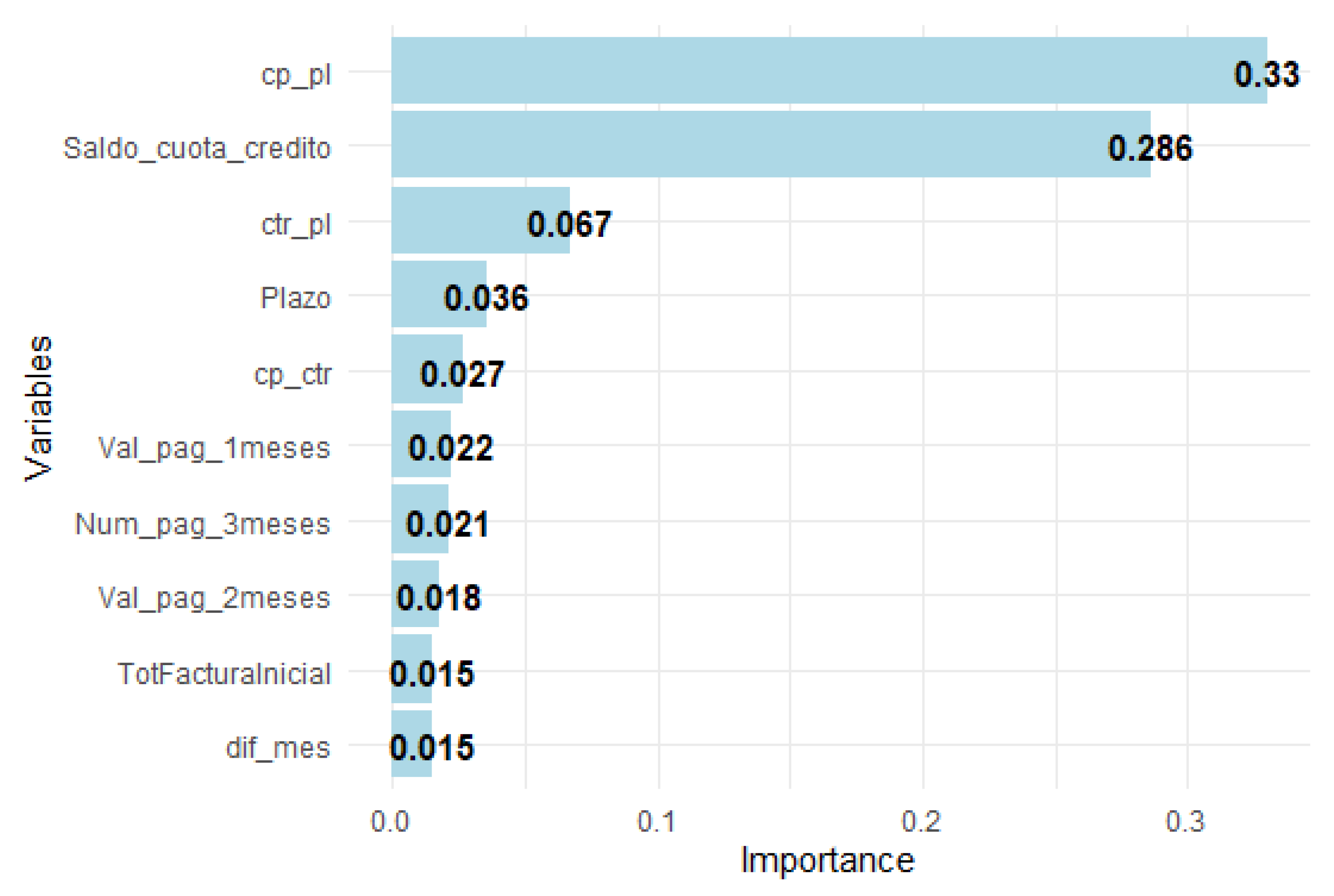
Figure A2.
Top 10 Important Variables in XGBoost 1-30 Segment Model.
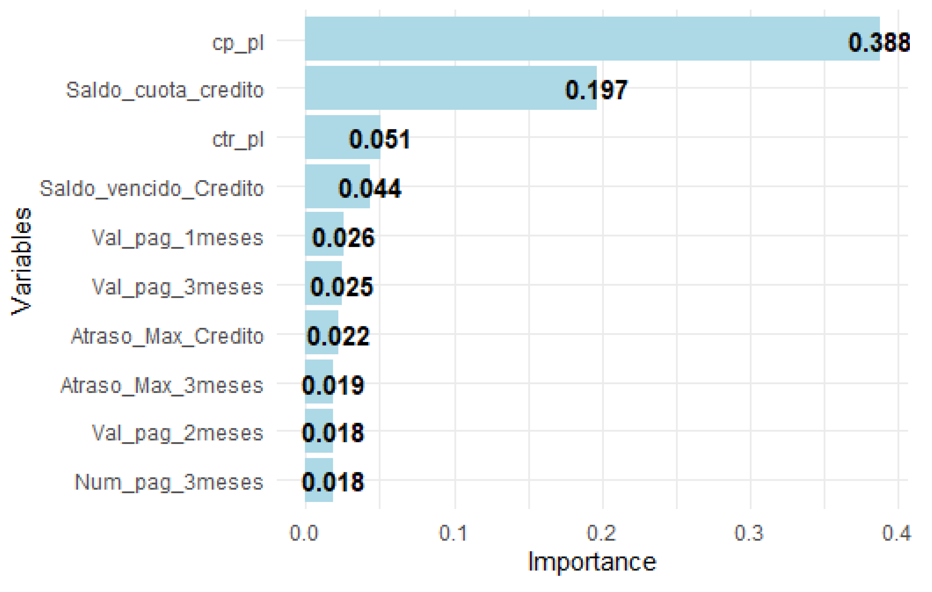
Figure A3.
Top 10 Important Variables in XGBoost 31-90 Segment Model.

References
- Arnold, T. B.; Emerson, J. W. Nonparametric goodness-of-fit tests for discrete null distributions. R Journal 2011, 3(2). [Google Scholar] [CrossRef]
- Bartz, E. , Bartz-Beielstein, T., Zaefferer, M., & Mersmann, O. (2023). Hyperparameter tuning for machine and deep learning with r: A practical guide. [CrossRef]
- Bussmann, N. , Giudici, P., Marinelli, D., & Papenbrock, J. 2021. Explainable machine learning in credit risk management. Computational Economics.
- Capelo Vinza, J. A. (2012). Modelo de aprobación de tarjetas de crédito en la población ecuatoriana bancarizada a través de una metodología analítica, 2012. [Google Scholar]
- Chen, T. , & Guestrin, C. 2016. Xgboost: A scalable tree boosting system. InProceedings of the 22nd acm sigkdd international conference on knowledge discovery and data mining (pp. 785–794).
- Chen, Y. , Wang, H., Han, Y., Feng, Y., & Lu, H. (2024). Comparison of machine learning models in credit risk assessment. ( 2024). Comparison of machine learning models in credit risk assessment. Applied and Computational Engineering74, 278–288.
- Chollet, F. 2018. Deep learning with R/François Chollet; with JJ Allaire. Deep learn. R.
- Cifuentes Baquero, N. , & Gutiérrez Murcia, L. (2022). Modelo predictivo de la probabilidad de aumento de los días de mora para usuarios de tarjeta de crédito.
- Deisenroth, M. P. , Faisal, A. A., & Ong, C. S. (2020). Mathematics for machine learning.
- Ertel, W. (2018). Introduction to artificial intelligence.
- Galindo, J. , & Tamayo, P. (2000). Credit risk assessment using statistical and machine learning: basic methodology and risk modeling applications. Computational economics, 15.
- Hernández, R. , Fernández, C., Baptista, P., et al. (2014). Metodología de la investigación, m: méxico.
- Iñiguez, C. , & Morales, M. (2009). Selección de perfiles de clientes mediante regresión logística para muestras desproporcionadas, validación, monitoreo y aplicación en la proyección de provisiones. Escuela Politécnica Nacional, Ecuador.
- Jácome Jara, M. S. (2014). Construcción de un modelo estadístico para calcular el riesgo de deterioro de una cartera de microcréditos y propuesta de un sistema de gestión para la recuperación de la cartera en una empresa de cobranzas, E: Quito, 2014. [Google Scholar]
- Lawrence, D. B. , & Solomon, A. (2002). Managing a consumer lending business. (No Title).
- Li, Z. Extracting spatial effects from machine learning model using local interpretation method: An example of SHAP and XGBoost. Computers, Environment and Urban Systems 96 2022, 96, 101845. [Google Scholar] [CrossRef]
- Maddala, G. S. , Contreras García, J., Lozano López, V., García Ferrer, A., et al. (1985). Econometría.
- Massey Jr, F. J. The Kolmogorov-Smirnov test for goodness of fit. Journal of the American statistical Association 1951, 46(253), 68–78. [Google Scholar] [CrossRef]
- Molnar, C. Interpretable machine learning. 2021. Available online: https://fedefliguer.github.io/AAI/redes-neuronales.html (accessed on day month year).
- Pérez Tatamués, A. E. (2014). Modelo de activación de tarjetas de crédito en el mercado crediticio ecuatoriano a través de una metodología analítica y automatizada en r, 2014. [Google Scholar]
- Reche, J. L. C. (2013). Regresión logística. Tratamiento computacional con R. Universidad de Granada.
- Sanchez Farfan, Y. S. (2023). Aplicación del modelo credit scoring y regresión logística en la predicción del crédito, en una entidad financiera de la ciudad del Cusco 2022.
- Suquillo Llumiquinga, J. A. Credit scoring: aplicando técnicas de regresión logística y modelos aditivos generalizados para una cartera de crédito en una entidad financiera. (B.S. thesis), Quito, 2021. [Google Scholar]
- Támara-Ayús, A. L.; Vargas-Ramírez, H.; Cuartas, J. J.; Chica-Arrieta, I. E. Regresión logística y redes neuronales como herramientas para realizar un modelo Scoring. Revista Lasallista de Investigación 2019, 16(1), 187–200. [Google Scholar] [CrossRef]
- Thomas, L.; Crook, J.; Edelman, D. Credit scoring and its applications; SIAM, 2017. [Google Scholar]
- Vargas Lara, D. O. Metodología para la obtención de un modelo de cobranza de créditos masivos. desarrollo y obtención de un modelo de scor. (Unpublished master’s thesis), Quito, 2015. [Google Scholar]
- Yeh, I.-C.; Lien, C.-h. Credit Scoring Using Machine Learning Techniques: A Review and Open Research Issues. Mathematics 2023, 11(4), 839. [Google Scholar] [CrossRef]
Figure 1.
Example of a Credit Collection Strategy.
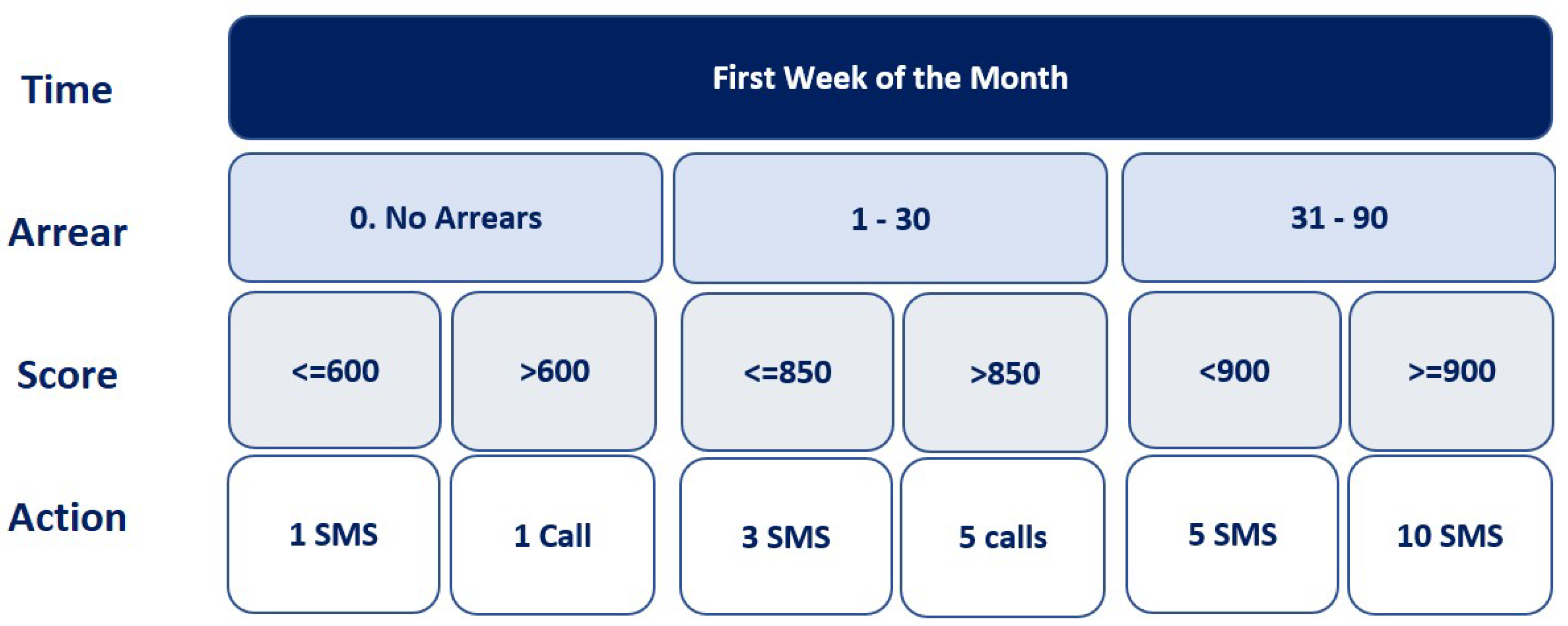
Figure 7.
Top 10 Important Variables in XGBoost No Arrears Segment Model.
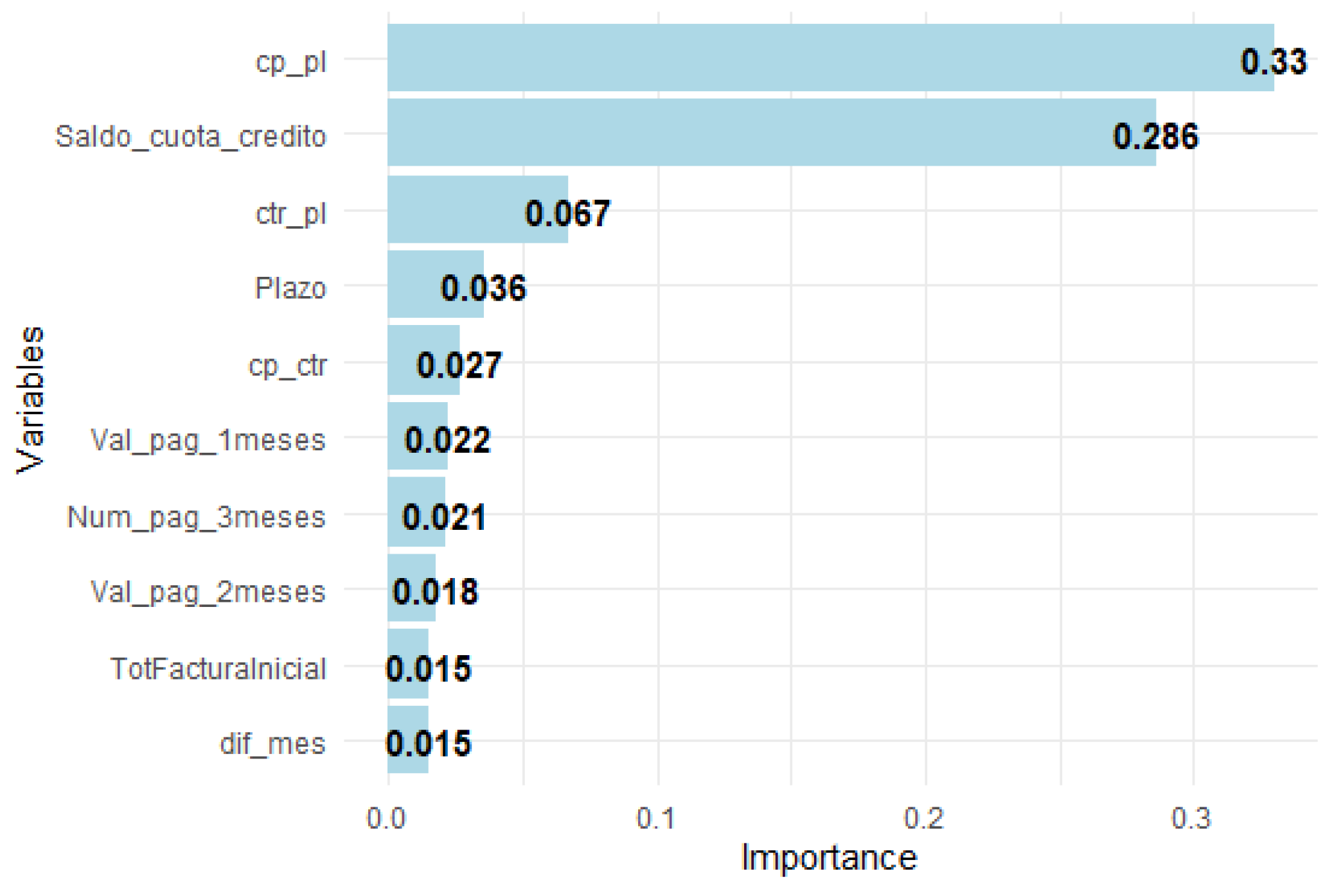
Table 1.
Distribution of the training, testing, and validation samples.
| Train | Test | Validation |
|---|---|---|
| 87,821 | 37,638 | 18,819 |
| 61% | 26% | 13% |
Table 2.
Distribution of customers classified as Good (G) and Bad (B).
| Dep.Var. | Arrears | Train | Test | Validation | |||
|---|---|---|---|---|---|---|---|
| G | B | G | B | G | B | ||
| Y1 | 0-no arrears | 75% | 25% | 75% | 25% | 75% | 25% |
| 1-30 | 68% | 32% | 68% | 32% | 67% | 33% | |
| 31-90 | 32% | 68% | 32% | 68% | 33% | 67% | |
| Y2 | All | 63% | 37% | 63% | 37% | 63% | 37% |
Table 3.
All Models KS Results by Arrears Segment.
| 0 Segment Models | 1–30 Segment Model | |||||
|---|---|---|---|---|---|---|
| LR | XGB | ANN | LR | XGB | ANN | |
| 56.42% | 63.36% | 61.84% | 47.32% | 51.38% | 50.35% | |
| 31–90 Segment Model | All Arrears Model | |||||
| LR | XGB | ANN | LR | XGB | ANN | |
| 36.62% | 34.47% | 38.77% | 71.01% | 74.05% | 73.59% | |
Disclaimer/Publisher’s Note: The statements, opinions and data contained in all publications are solely those of the individual author(s) and contributor(s) and not of MDPI and/or the editor(s). MDPI and/or the editor(s) disclaim responsibility for any injury to people or property resulting from any ideas, methods, instructions or products referred to in the content. |
© 2025 by the authors. Licensee MDPI, Basel, Switzerland. This article is an open access article distributed under the terms and conditions of the Creative Commons Attribution (CC BY) license (http://creativecommons.org/licenses/by/4.0/).
Copyright: This open access article is published under a Creative Commons CC BY 4.0 license, which permit the free download, distribution, and reuse, provided that the author and preprint are cited in any reuse.


