
Submitted:
07 July 2025
Posted:
08 July 2025
You are already at the latest version
Abstract
This paper deals with the design and the robustness analysis of a Model Predictive Control (MPC) for the position tracking of primary flight movables driven by elec-tro-mechanical actuators. The study is in particular focused on a rotary Elec-tro-Mechanical Actuator (EMA) by UMBRAGROUP, employing a patented mechanical transmission based on differential ball-screw mechanism characterized by huge gear ratio. To obtain a baseline reference, conventional PID regulators have been initially optimized by using multi-objective cost functions based on tracking accuracy, load disturbance rejection and power consumption. The position regulator has been then replaced by an MPC regulator, designed to balance performance, computational re-sources and safety constraints. A nonlinear physics-based simulation model of the EMA, entirely developed in the Matlab-Simulink environment and validated with ex-periments, has been used to compare the two control strategies. Simulation results in both time and frequency domains highlight that the MPC solution provides faster and more accurate position tracking, improved dynamic stiffness and reduced power ab-sorption. Finally, the robustness against model uncertainties of the MPC is addressed, by imposing random and combined deviations of model parameters from the nominal values (via Monte Carlo analysis). The results demonstrate that the implementation of MPC control laws could enhance the stability and the reliability of EMAs, thus sup-porting their application for safety-critical flight control functions.
Keywords:
electro-mechanical actuators
; model predictive control
; optimal control
; modelling
; simulation
; flight control
1. Introduction
In recent years, the aerospace sector has undergone a progressive shift toward the electrification of onboard systems, driven by the need to improve energy efficiency, reduce environmental impact, and optimize system integration [1]. The More Electric Aircraft (MEA) concept seeks to replace traditional hydraulic and pneumatic systems with electrically powered alternatives, offering benefits in terms of weight reduction, maintenance costs, and sustainability [2,3,4]. Nevertheless, given the present power density storage technology [5], the feasibility of achieving the All Electric Aircraft (AEA) is currently limited to Urban Air Mobility (UAM) applications, such as the emerging market of Urban Air Taxi (UAT) and electrical Vertical Take-Off and Landing (eVTOL) vehicles [6]. A key enabling technology within this transformation is the Electro-Mechanical Actuator [7], which converts electrical energy into mechanical motion using an electric motor and a mechanical transmission, hence without relying on hydraulic fluids, eliminating leakage risks and simplifying system architecture. Significant progress in enabling components—such as electric machines [8], power electronics [9], and materials of mechanical elements [10]—has notably increased the Technology Readiness Level (TRL) of these systems. Although the feasibility of EMAs in aerospace applications has been demonstrated in terms of load capacity, dynamic performance, and health monitoring capabilities [11,12,13,14,15], the deployment on safety-critical flight controls or landing gears still raises concerns related to reliability, fault tolerance, and compliance with airworthiness certification standards [16,17]. To address these functions, several architectural solutions have been proposed, including simplex configurations with passive fail-safe mechanisms and more complex redundant fault-tolerant architectures involving dual motors, independent control paths, or differential mechanisms. Nevertheless, actuator reliability depends not only on hardware redundancy but also on the control and monitoring strategies implemented [18]. Robust and high-performance controllers are essential to ensure system stability and disturbance rejection under variable conditions and partial faults [19]. Classical control approaches, such as Proportional-Integral (PI) or Linear Quadratic Regulator (LQR) schemes, are widely employed in aerospace applications due to their simplicity, reliability and deterministic behaviour. However, these methods operate on current or past states and measurements, hence limited in managing future disturbances or constraints. In contrast, Model Predictive Control has emerged as a powerful alternative, enabling the anticipation of future system behaviour through internal prediction models and the explicit handling of input and state constraints within the control action optimization window [20]. Eren et al. [22] provide a comprehensive review of MPC techniques for aircraft and spacecraft systems applications, focusing on safety-critical applications and fault-tolerant control, observing that the complexity of nonlinear formulations is a challenge for practical implementation in safety-critical functions. Although RTCA DO-178C does not restrict the choice of control techniques from a certification standpoint [23], the software implementation of PI controllers is generally easier to validate due to their interpretability and limited branching logic, making Modified Condition/Decision Coverage (MC/DC) relatively straightforward. In contrast, for MPC involving model nonlinearities or constrained real-time optimization, the highly complex logic, numerical challenges, and recursive solver behaviour may significantly increase the verification effort—particularly in applications subject to higher Development Assurance Level (DAL) classification.
MPC has been studied in the context of aircraft flight mechanics for load alleviation functions [24] and dynamic system modelling [25], spacecraft enhancement dynamics [26], and UAVs manoeuvres optimization [27,28]. MPC has also demonstrated promising results in governing Permanent Magnet Synchronous Motors (PMSM), functioning as a speed controller [29], MIMO Direct-Quadrature currents regulator [30], and direct torque controller (DTC) [31]. Additionally, Hasan et al. [32] employed MPC as a speed regulator for electromagnetic actuators, integrated with a PI position controller. Nevertheless, the use of MPC for position control in safety-critical EMAs remains a promising yet open research topic. The main barriers are associated with the nonlinear and coupled dynamics of electro-mechanical systems, the need for real-time implementation on embedded hardware with limited computational resources, and the rigorous certification requirements in aviation environments.
The main objective of this work is to assess the feasibility and advantages of applying MPC to a rotary EMA developed by UMBRAGROUP for primary flight control applications, by comparing its performance and robustness with those of conventional control laws.
The paper is articulated as follows: the first part is dedicated to the description of the EMA architecture and to the development of a detailed model integrating both electrical and mechanical subsystems from first physical principles. Subsequently, the classical PI-based cascade of position, speed and current regulators is designed through a multi-objectives optimization. A Linear Time Invariant (LTI) MPC then replaces the PI position regulator, while keeping other loops unchanged. Comprehensive simulations with a nonlinear model in Simulink assess the performance of PI- and MPC-controlled EMAs in time and frequency domains, also evaluating robustness against individual and coupled parameters deviations and model uncertainties, as well as the power absorption and computational resource requirements. Finally, key findings are discussed, highlighting differences between the two approaches, along with suggestions for future refinements.
2. Materials and Methods
2.1. System Description
The reference architecture for this study is a rotary fail-safe EMA (Figure 1), based on a differential ball-screw patented by UMBRAGROUP (UG) [33], within the CleanSky 2 program [34]. The closed-loop control of EMAs designed for secondary flight surfaces primarily focuses on disturbance rejection requirements, minimizing position deviations from the commanded setpoint when external loads act on the surface. Conversely, the position tracking behaviour under load is the key performance requirement that an actuator specifically designed for primary flight controls must meet. In this last case, the position control loop should operate at higher bandwidths (e.g., 2–10 Hz), ensuring precise tracking, while the output shaft speed typically ranges between 10 and 60 degrees per second.
The specific case study investigates the rotary EMA architecture integrated into the rudder actuation system of a medium-sized eVTOL vehicle featuring a V-tail configuration. In such a layout, the rudder functions as a primary flight control surface, contributing to both yaw and pitch control during cruise and transition phases. Consequently, the actuator must ensure high dynamic performance, particularly in terms of frequency response, position tracking accuracy, and robustness against aerodynamic disturbances.
2.2. System Dynamics Modelling
High-fidelity nonlinear models of EMAs are widely used to accurately reproduce the behaviour of the real system. Such model-based approaches have become increasingly relevant in the context of digital twin development, enabling simulation-based analysis and verification for monitoring and control algorithms. The developed nonlinear model of the EMA, illustrated in Figure 2, includes two main sections: the electro-mechanical section and the digital electronics section, each comprising multiple functional blocks. The electro-mechanical section consists of the following components:
- Three-phase Surface mounted Permanent Magnet Synchronous Motor (S-PMSM) current dynamics in the direct-quadrature (d-q) reference frame;
- UMBRAGROUP patented mechanical transmission based on a high transmission ratio differential ball-screw mechanism, including its internal stiffness and resonance;
- Coulomb and viscous friction;
- Rotational dynamics of the output shaft, including the reference aircraft surface inertia and external load effects.
The digital electronics section includes:
- Three nested control loops acting on motor direct and quadrature currents, motor speed, and output shaft position;
- Control nonlinearities (saturations, rate-limiter on position command);
- Sensors dynamics, latencies and resolution;
- Resolver sensors for motor and output shaft position feedback;
- Motor speed reconstruction from angular position;
- Hall-effect sensors for current measurement;
- Digital signal processing performed at 10 kHz.
The model is implemented in Simulink using the ODE4 Runge-Kutta solver with a fixed integration step of 10-5 s.
2.2.1. Electro-Mechanical Section
The electro-mechanical section includes three main dynamic contributions: the electric motor with d-q axes current dynamics (1), the rotor-side one degree of freedom (DOF) rotational motion (2) and the output shaft with 1-DOF rotational dynamics (3). These equations are coupled through the compliant mechanical transmission, modelled with lumped spring-damper parameters, assuming low structural damping.
Vd, Vq and Id, Iq are respectively the direct and quadrature voltages and currents. Lph and Rph are the motor phase inductance and resistance, nd is the number of pole pairs, and Ke is the back-electromotive force constant of the PMSM. θm and θo are respectively the angular positions of the motor and the output shaft, and Jm and Jo are the associated inertias. Kg and Cg represent the torsional stiffness and damping of the differential ball-screw drivetrain with gear ratio τg. The motor torque constant kt is equal to Ke for S-PMSM. Bm is the viscous friction coefficient, while Tc and ωc are the parameters of the Coulomb-tanh friction model illustrated in Figure 3. Finally, Text is the external torque acting on the output shaft, accounting for load disturbances and aerodynamic actions.
The proposed model represents a balance between accuracy and complexity, consistent with the current objective of comparing control strategies rather than developing a high-fidelity simulation framework. More advanced EMA models usually include three-phase current dynamics, with Space Vector Pulse Width Modulation (SVPWM) and field-oriented control (FOC) [35], to represent real-time switching behaviour accurately. PMSM iron losses, detailed friction models and sensor noise were not included, since experimentally identified data were not available; however, these effects would impact both controllers equally. The parameters used in the electro-mechanical section of the simulation model are listed in Table 1.
2.2.2. Digital Electronics Section
The digital control section of the model includes two main main parts.
- Control laws: the EMA output position command is first rate-limited at the maximum output shaft speed ωomax, then compared to the resolver feedback. The position error is fed to the position regulator which generates a motor speed request. This is compared to the value derived from the motor resolver position feedback and fed to the motor speed regulator which outputs a quadrature current demand. The direct current instead has a fixed null reference to achieve Maximum Torque Per Ampere (MTPA) control for S-PMSM [36], assuming Ld = Lq = Lph. On the baseline design, position, speed and current regulators have a Proportional-Integral structure with saturation and anti-windup scheme. In the MPC-based control, only the position regulator is replaced with an MPC, maintaining the other control laws unchanged. Additionally, current regulator integrates the decoupling technique. By reformulating eq. (1), the relationships in (4) can be established, linking the voltages Vdreg, Vqreg, calculated by the current regulator, to their post-decoupling counterparts Vddec, Vqdec. This approach ensures that the current dynamics along the d-q axes remain unaffected by motor speed variations, leading to independent behaviour of the d and q currents. The equation (4) assumes that discrepancies between actual and measured values of currents and speed remain minimal, alongside with low variations in electrical constants, thus ensuring an effective decoupling. Finally, the voltages are dynamically saturated according to the constraint (5).
- Sensors processing: the rotor and output shaft positions are measured through resolver angular sensors, while d-q currents are acquired with Hall-effect current sensors. On the real EMA, each motor phase current is measured, then d-q currents are calculated in the digital control section via Clarke-Park transformation (6).
Sensor dynamics are modelled via continuous-time first order low-pass filters, whose characteristics are reported in Table 2. Sensor feedback are then digitized with sample and hold functions at 10 kHz rate.
2.3. Conventional control Laws Optimization
Conventional Proportional-Integral controllers are commonly used for their simplicity and capability to achieve zero steady-state tracking error. The general continuous-time transfer function is given by equation (7).
The two parameters (for each control loop) to be selected are:
- the proportional gain: KP;
- the zero of the integrator: zI.
These parameters are tuned to meet the stability and closed-loop performance requirements reported in Table 3. It is worth noting that the bandwidths of the three control loops are designed to be separated by one decade, in order to obtain disjointed dynamics.
PI controllers are designed through an optimization procedure based on a reduced-order Linear Time-Invariant model of the EMA, derived from equations (1)–(4) by imposing zero Coulomb friction, since its linearization would generate unrealistically high values for ω > ωc, and by neglecting the d-current dynamics (i.e. using a mono-phase equivalent model of the electrical machine (8)). Figure 4 illustrates the key degrees of freedom of this reduced electro-mechanical model.
This approach enables the systematic definition and minimization of performance-oriented cost functions, with the goal of identifying the optimal controller parameters that guarantee accurate position tracking and effective load disturbance rejection with minimal energy consumption. This also provides a consistent basis for comparison with the MPC-based control strategy. The controller design is framed as a multi-objective optimization problem, where each cost function Ji quantifies a specific performance metric of the EMA under predefined test conditions. A total of six cost functions are defined based on the EMA response in the following two scenarios:
- Position tracking test: the commanded output position is a step of θos = 1 deg, with no external load applied. The cost function measures the squared tracking error between the output position and the reference command (9). Similarly, is linked to the deviation of the motor speed from the regulator reference (10). The cost function quantifies the normalized electric power absorption: since it includes the open-loop input voltage Vq, this metric reflects the required effort to achieve the desired tracking performance.
- Load disturbance rejection test: the position command is set to the equilibrium condition (i.e. θocmd = 0 deg) while an external torque step of Text = 1 Nm is applied. The three corresponding cost functions are analogously defined (12)-(14).
Finally, the global cost function is defined as a weighted linear combination of the individual terms Ji, normalized by their respective minimum values to ensure comparability among different metrics (15). The minimum of equation (15) yields the optimal placement of the PI controller zeros.
To facilitate further results interpretation and to clarify the adopted weight assignment convention, it is useful to group each pair of cost functions associated to a specific performance metric: position tracking (16), speed tracking (17) and power consumption (18).
The controller optimization is carried out in the MATLAB environment, based on a state-space representation of the EMA LTI model. The procedure consists of the following main steps:
- Zeros placement variation: a common variation vector for zero placement is defined and applied equally across all control loops. The zeros location is varied as fractions of the respective closed-loop design bandwidths, within the range [0.1–0.5], to ensure a minimal impact of the zero on the bandwidth itself. Adopting a Monte Carlo-like optimization algorithm, a large number of zeros placement combinations are generated for the three nested control loops.
- Feed-forward design and stability verification: for each configuration, the feed-forward transfer function is constructed by cascading with the open-loop transfer function from its output to the EMA system output in the corresponding control loop. The proportional gain is then automatically calculated by enforcing that the cut-off frequency of the feed-forward transfer function matches the predefined closed-loop bandwidth. Stability margins are checked, and if they meet the required specifications, the state-space LTI closed-loop model of the EMA system is constructed.
- Time-domain simulation and cost functions evaluation: the position closed-loop EMA is simulated under position tracking and disturbance rejection tests; consequently, the values of the six cost functions are evaluated for each zeros configuration.
- Normalization of cost functions: for each cost function, the minimum value across all combinations is identified to allow its normalization. This ensures consistent comparison across metrics with different physical units and scales.
- Weight definition for multi-objectives cost function: given the focus on primary flight control applications, the optimization strategy prioritizes position tracking performance over secondary objectives. Accordingly, the weights associated with motor speed tracking and power consumption are fixed to small values (19); conversely, the weights associated with position tracking cost functions are allowed to vary within a discrete set of values (20) to be treated as tuneable parameters within the optimization process.
Only combinations satisfying the constraint are valid. This approach effectively incorporates weights tuning into the overall optimization framework, thereby expanding the dimensionality of the parameters space and enabling a balanced trade-off among the multiple performance objectives.
- 6.
- Computation of the global cost function: for each valid combination of zero placements and cost function weights, the global cost function Jw is evaluated according to (15).
- 7.
- Optimal design identification: the optimal controllers configuration is identified as the one that minimizes the global cost function, ensuring the best trade-off among the considered performance metrics.
2.4. Model Predictive Controller development
An MPC for EMA position regulation was developed based on the standard theory of discrete-time, LTI, state-space formulation for single-input-single-output model-based predictive control [37]. This control approach represents a novel strategy in aerospace EMA applications. Its objective is to optimize the system performance by predicting future behaviour and computing control actions accordingly. This technique relies on a dynamic model of the plant and solves an optimization problem at each time step to minimize a cost function while satisfying system constraints. The implementation of an MPC algorithm requires the following elements:
- Information on the current and previous states of the system;
- A mathematical model of the plant to predict its future evolution;
- An optimization criterion (typically a quadratic cost function).
The MPC strategy is based on three core concepts, displayed in Figure 5:
- Prediction Horizon (Np) defines the finite time span (in terms of discrete time steps k) over which the future system output is predicted, using the plant model and current state information. A longer prediction horizon allows the controller to capture a more comprehensive understanding of the system evolution, though increasing the complexity of the algorithm.
- Control Horizon (Nc) denotes the finite time window over which the future control inputs u(k) are optimized, i.e. for k=ki,…,ki+Nc-1, where ki is the initial time. Nc is constrained by computational costs and the need to balance predictive accuracy with real-time implementation. Thus, Nc is usually smaller than Np , and for k>ki+Nc-1 the control input is assumed to remain constant. The selection of an appropriate control horizon is crucial as it directly influences the controller ability to anticipate and regulate the system behaviour effectively.
- Receding Horizon control: a dynamic optimization framework enables the controller to adapt its control strategy in real-time by recalculating control inputs at each time step, based on the most recent state information, to enhance robustness against model inaccuracies and external perturbations and to maintain system stability. Mathematically, at time k, the MPC computes an optimal sequence of control actions over the full control horizon, however, only the first input u(k) is applied to the plant. At the next time step, the system state is updated, and a new optimization is performed.
2.4.1. Discrete-time LTI MPC formulation
The design of a Model Predictive Controller is based on a mathematical model of the plant, with its algorithm complexity increasing as the model becomes more detailed or nonlinear. A basic MPC formulation relies on a discrete-time, LTI, SISO, state-space model (the extension to multiple-input multiple-output (MIMO) systems is straightforward), which embedded dynamic equations are formulated as (21), (22), where k is the actual time sample, xm(k) is the vector of states at time k with length n1, u(k) and y(k) are respectively the input and output at the current time (both scalar for SISO), Am(n1 x n1), Bm(n1 x 1) and Cm(1 x n1) are the plant state-space representation matrices with constant parameters. Due to the receding horizon technique, the Dm matrix is always null, since the input cannot affect directly the output at the same time step. If the dynamic model is nonlinear, the matrices can be obtained via linearization around an equilibrium point.
Expressing the variation of the input and states within two consecutive time samples (23), it is possible to rearrange the dynamic equations (21),(22) in incremental terms (24),(25).
Defining the so-called augmented states vector (26), the augmented state-space LTI model of the plant is obtained (27)-(29) used to design the MPC controller and for the calculation of future states and outputs.
2.4.2. Prediction Within One Optimization Window
At each discrete time step ki > 0, the MPC algorithm solves an optimization problem to compute the Nc future increments of the control variable Δu(ki),…,Δu(ki + Nc - 1). Based on this control sequence, using the augmented model, the algorithm then predicts sequentially the future states (30), and the output (31) of the system over the prediction horizon Np (i.e. the optimization window). The notation x(k | ki) denotes the predicted state for future time k = ki + 1, …, ki + Np carried out at time ki. By defining two vectors containing all Np values of input (32) and output (33), the dynamic equation used for output prediction can be rewritten in a compact, state-space-like form (34). Remarkably, the F and Φ matrices depend only on the augmented model matrices, defined as constant, enabling a significant simplification of the MPC code generation.
2.4.3. Optimization Criterion
The control objective of the MPC is to minimize the deviation between the predicted output and a reference signal r(ki), which is assumed to remain constant over the prediction horizon (35). This goal is achieved by computing the optimal sequence of control increments ΔU that minimizes a convex quadratic cost function (36). The first part aims to minimize the tracking error e(ki) = r(ki) – y(ki), while the second term penalizes excessive control effort by weighting the magnitude of ΔU. This trade-off is regulated by a tuneable parameter rw ≥ 0, embedded in the diagonal input-weighting matrix , where is the identity matrix. The input-weight parameter rw governs the balance between tracking performance and control effort. Setting rw = 0 results in a purely performance-oriented controller, neglecting the cost of control variation. Conversely, larger rw values yield smoother control inputs by limiting abrupt variations, thus producing a more conservative response.
By substituting equation (34) into (36), the expanded expression shown in (37) is obtained.
By setting the gradient of the cost function with respect to ΔU to zero, and considering the problem’s convex and quadratic structure, a unique global minimum is guaranteed, which corresponds to the optimal control trajectory (38). The term in (38) is commonly referred to as the Hessian matrix, whose existence is guaranteed by the problem construction. Since both Φ and are constant matrices in this formulation, the resulting Hessian matrix is also constant.
2.4.4. Model Predictive Position Controller Design
The first design decision involves choosing how to integrate the Model Predictive Controller: since classical EMA architectures consist of three nested loops, one option would be to replace all of them with a single MPC regulator. However, this strategy introduces significant challenges: internal saturation limits (e.g., maximum motor speed and current), typically enforced by external saturation blocks, must be explicitly addresses as hard constraints on system states, inputs and outputs. This approach would require solving a constrained optimization problem with linear inequalities constraints. Although MPC algorithms can address this task using Quadratic Programming methods such as Hildreth’s algorithm [38], the associated computational complexity and potential constraints conflicts make this solution unsuitable for safety-critical applications. Preliminary control laws design and further optimization of PI controllers highlighted a strong dependence of the EMA closed-loop performance on the tuning of the position regulator, while motor speed and current regulators have a secondary influence. Based on these evidence, the MPC was employed as the position regulator, in cascade with the optimized PI controllers for speed and current loops. Aerospace applications impose a trade-off between embedded model accuracy and necessary computational resources: certification requirements in safety-critical systems limit the use of complex or unverified algorithms. Therefore, the embedded model must be kept as simple as possible while still capturing the essential EMA dynamics. To fulfil these requirements, the MPC was developed without internal constraints and based on a simplified LTI model. Specifically, since the MPC operates as a position regulator, its embedded model corresponds to the speed closed-loop EMA shown in Figure 6, represented by the transfer function (39) and discretized at a 10 kHz sampling rate. Referring to Figure 6, the open-loop model of the EMA corresponds to the five-states representation used also for PIs optimization (Figure 4). The inclusion of current and speed loops integrators adds two additional states. An additional state results from the discrete-time derivative and filtering used in speed reconstruction, yielding a total of eight states (40). These additional states are not directly measurable but can be computed from the PI regulators' internal variables and sensor processing at the previous time step. The output speed ωo is estimated using the same approach applied to calculate the motor speed from the position feedback.
In the absence of a formal procedure to determine an optimal configuration for MPC parameters (Nc, Np and rw) a-priori, the design was carried out through an iterative refinement. A series of closed-loop simulations were conducted, progressively adjusting the tuning parameters based on the observed performance, until satisfactory tracking accuracy and closed-loop stability were achieved with minimal control effort. This iterative process led to some key considerations:
- a short control horizon (Nc = 5) proved sufficient, as longer values did not significantly improve performance;
- a long prediction horizon (Np = 500) was necessary to properly capture the system dynamics and generate effective control actions;
- Given the incremental nature of the MPC law, the input-weighting factor should remain small (rw = 10-3) to prevent over-smooth inputs, thereby preserving actuator responsiveness and ensuring adequate control authority.
In the nonlinear Simulink model, the MPC is implemented via a custom MATLAB function that computes the optimal control trajectory as expressed in (38). The necessary matrices (41), being constant in this formulation, are precomputed and loaded into the code. By opting for a significantly reduced control horizon, these matrices are of small dimension. To compute ΔUopt, the MPC block requires the reference input r(k) = θocmd(k) and the augmented states vector (26); therefore, state values at both the current and previous time steps are needed. Finally, the MPC applies only the first element of the control increment vector to compute the optimal speed reference, as defined in equation (42). Finally, the MPC output is externally saturated, to avoid a more complex constrained optimization procedure, and it is sent to the motor speed regulator in cascade.
2.5. Performance Comparison and Robustness Analysis
To substantiate the differences between the two control strategies, the following simulations in time and frequency domain have been performed.
- The EMA unloaded position tracking response is assessed in the frequency domain with harmonic commands of 1 deg amplitude.
- In the loaded position tracking tests, aerodynamic actions on the control surface are modelled as an equivalent torsional spring with constant stiffness Kaero, acting on the EMA output shaft (43).
The tests are conducted using sinusoidal commands with amplitudes of 0.1 deg, 1 deg and 10 deg.
- 3.
- The EMA dynamic compliance is derived imposing harmonic and step-like loads of 1 Nm amplitude.
To quantify the energetic benefit of MPC, the percentage energy reduction is defined as in (44), where the energy terms (EMPC, EPI) are evaluated according to the respective power integral (45).
To assess the robustness of the control strategies, a reference test sequence is designed. The actuator is first commanded to track and hold a 1 deg position step command under aerodynamic spring-load. Subsequently, an external load step of 1 Nm is applied on the output shaft to evaluate the ability to reject gust disturbances. The robustness analysis is conducted in two phases. First, a comprehensive single-parameter sensitivity analysis is carried out by individually varying several parameters of the EMA nonlinear model. Due to the high inherent robustness of both controllers, only the most relevant results are reported, related to the variation of the following parameters:
- PMSM torque constant kt ;
- friction torque multiplier Kf ;
- equivalent aerodynamic spring load stiffness Kaero.
Figure 7 displays the ten selected points for each parameter along with their mean values (used as baseline) and the standard deviation.
As a second step, focusing on MPC, a multi-parameter robustness analysis is performed to account for potential nonlinear interactions among uncertainties. A Monte Carlo-like approach is employed to generate 103 combinations of the parameters above. The MPC robustness is then evaluated in comparison to the baseline performance. Key statistics metrics include the deviation of the position tracking error (46) and the deviation in the electrical power consumption (47), providing a quantitative assessment of tracking accuracy and energy efficiency under uncertainty. For each Monte Carlo run and for both performance metrics, the four statistical moments (the mean, the standard deviation, the skewness and the kurtosis) are computed over the simulation timespan Nsim. This analysis intended to support a statistical robustness evaluation by estimating the likely distribution of performance metrics across a representative range of uncertain conditions.
3. Results
3.1. Proportional-Integral Controllers Optimization
Figure 8, Figure 9 and Figure 10 provide a concise overview of the main trends observed in the PI cost functions. Figure 8 shows the individual cost terms plotted against the normalised locations of the zeros placement: the x axis reports , the y axis , and the different surfaces correspond to different values of . Results from both the position-tracking and disturbance-rejection tests suggested that, for each performance metric, the corresponding pair of cost functions exhibit similar trend, hence the definitions (16)-(18) illustrated in Figure 9. Conversely, position- and speed-related cost functions displayed opposite trends: combinations that minimizes inevitably increased , emphasising the necessity of a multi-objectives optimization. The current loop zero had only a marginal influence on the power cost index of disturbance rejection tests. Finally, Figure 10 locates every controller design in the three-dimensional space (, , ). The plane (48) is tangent to the Pareto front of the multi-objective optimization exactly at a single point (highlighted), which therefore represents the global optimum and the recommended zero placement configuration for PIs design, reported numerically in Table 4.
3.2. PI and MPC-Based Control Performance Comparison
3.2.1. Unloaded Position Tracking Tests
The Bode diagram in Figure 11 compares the MPC- and PI-based systems frequency responses during unloaded position tracking tests. The acceptance mask for the frequency response is defined as follows.
- At frequencies lower than 0.2 Hz the magnitude shall remain within ±1 dB, while the phase shall be higher than -10 deg.
- For frequencies between 0.2 Hz and 2 Hz, a linear increase in the magnitude is allowed till ±3 dB at the design bandwidth, whereas the phase shall remain above -60 deg.
- Beyond 2 Hz the magnitude is expected to decay with a slope between –20 dB/dec and –40 dB/dec, while the phase must be greater than -180 deg.
While both architectures achieved the nominal position-loop bandwidth, the MPC-controlled EMA exhibited a flatter gain profile and reduced phase lag up to approximately 6 Hz, suggesting enhanced dynamic performance.
The computational effort required by both control strategies was evaluated through a one-second simulation with step-like position command, performed under identical hardware conditions. Execution times were comparable (1.77 s for the PI and 1.83 s for the MPC), indicating the feasibility of MPC real-time implementation without extra processing resources.
3.2.2. Loaded Position Tracking Tests
Figure 12 shows the loaded frequency response at increasing levels of command amplitude. At 0.1 deg, typical of aircraft stability augmentation functions, the PI controller suffered early gain attenuation and phase lag, while MPC maintained full sensitivity at small commands. At 1 deg, representative of typical autopilot commands, both controllers met the performance requirements. Under extreme manoeuvres (10 deg), saturation effects caused both to exceed the acceptance limits.
3.2.3. Load Disturbance Rejection Tests
The response of the EMA to a step-like gust disturbance is shown Figure 13. Despite a comparable peak in output position, the MPC-controlled actuator returned to equilibrium significantly faster, demonstrating superior damping. This improved rejection capability was further confirmed by the motor speed and current profiles: while PI induced strong oscillations, the MPC ensured smoother transients. In addition, energy consumption was reduced by 20%, highlighting MPC as a promising solution also for aircraft secondary control surfaces.
The Bode diagram of the EMA dynamic compliance, defined as the transfer function from external torque input to the angular displacement, is illustrated in Figure 14. Around the design bandwidth, the MPC achieved slightly greater load attenuation and a higher phase lead, enabling faster compensation of the disturbance. At low frequencies, PI outperformed MPC due to better phase anticipation. In the high frequency range, the responses of the two controllers converged, as the actuator resonance mode dominated the overall dynamics.
3.3. Robustness Analysis
The time-domain responses of MPC- and PI-controlled EMAs under single-parameter variation are illustrated in Figure 15, Figure 16 and Figure 17. Considering the variation of the motor torque constant (Figure 15), both control strategies exhibited strong robustness in the output position response. However, significant sensitivity is observed in the electrical quantities. At lower values of the torque constant kt, a higher quadrature current is required to generate the same motor torque, resulting in increased power peaks in both systems. Nevertheless, in this extreme scenario, the relative energy saving achieved by the MPC strategy became even more evident, highlighting its superior efficiency.
Uncertainty in the friction coefficients (Figure 16) introduced noticeable deviations not only in the electrical but also in the mechanical responses. Deviations in the output position became significant, particularly for the PI controller, highlighting its higher sensitivity to friction-induced drag. The MPC controller, instead, exhibited improved consistency in position tracking and faster recovery following the disturbance, while showing reduced energy consumption, especially under severe parameter deviations.
Unlike the previous cases, variations in Kaero influenced the external load model rather than the intrinsic characteristics of the actuator. The MPC controller was able to leverage this variation more effectively, progressively enhancing its energy efficiency from the unloaded condition up to the maximum aerodynamic load.
The second phase of the analysis focused on a detailed robustness characterization of the MPC with respect to combined variations of the parameters kt, Kf and Kaero. Figure 18 shows the statistical distribution of the position error deviation across all Monte Carlo simulations, in terms of mean, standard deviation, skewness, and kurtosis. The distribution of the mean value, centered near zero with a slight positive bias, indicated that tracking performance is generally preserved. The standard deviation revealed a multi-modal profile, suggesting the presence of distinct sensitivity clusters due to the discrete influence of the Kaero. Skewness values were broadly distributed around zero, showing no dominant direction asymmetry. The high kurtosis observed across the dataset confirmed a leptokurtic distribution, characterized by a non-negligible occurrence of extreme outliers. These cases represented critical parameter combinations that lead to significant deviations in tracking performance.
To better understand the interaction between uncertain parameters and their impact on control performance, the statistical metrics of the position error deviation were mapped over the kt - Kf plane and layered with Kaero values (Figure 19). The mean and standard deviation plots revealed a reduction in control effectiveness under conditions of low electro-mechanical coupling combined with high friction and external loads.
The power consumption deviation metrics are summarized in Figure 20. The distribution of the mean value was predominantly non-negative and slightly right-skewed, indicating that most uncertain configurations tend to increase average power consumption compared to the nominal scenario. Notably, a secondary mode with negative values emerged, suggesting that a subset of parameter combinations can also lead to net energy savings. This behaviour aligned with the bimodal trend observed in the skewness plot. The heavy-tailed standard deviation suggested nonlinear amplification of power fluctuations under uncertainty. The kurtosis appeared strongly leptokurtic, with frequent extreme outliers. This reflected the system susceptibility to large energetic deviations under specific uncertainty conditions, in contrast to the more constrained behaviour observed in the position error analysis.
Figure 21 is useful for identifying specific regions where strong power performance degradation occurred. Similarly to the position trend, the mean and standard deviation increased significantly for low kt and high Kf, highlighting a critical region for EMA robustness. Skewness confirmed highly asymmetric and heavy-tailed behaviour in the same region. Interestingly, the combined influence of extreme values of Kaero and kt appeared secondary in terms of mean and standard deviation but had a significant impact on kurtosis, suggesting that certain parameter combinations might have amplified rare yet extreme power deviations.
4. Discussion
This study provides a comprehensive assessment of the performance and robustness of conventional PI-based and advanced MPC strategies applied to an electromechanical actuator for primary flight control surfaces. The findings highlight distinct response patterns between conventional PI-based and model predictive control strategies, driven by their respective structural characteristics and interaction with system dynamics. To ensure a fair assessment, the baseline PI controller was first tuned through a multi-objective optimization procedure, balancing dynamic response and power consumption. Nevertheless, the MPC controller consistently outperformed the PI architecture in terms of both dynamic response and energy efficiency, across test scenarios representative of primary and secondary flight control applications. Notably, this was obtained without a significant increase in computational cost, as simulation times remained comparable.
The comparison of PI and MPC robustness under single-parameter variations highlighted a major degradation in PI performance under high friction, low torque constant, and stiff aerodynamic loads. In contrast, the MPC demonstrated greater overall stability, enabled by its predictive formulation, even relying on a non-adaptive embedded model.
Robustness characterization of the MPC design was further assessed via Monte Carlo analysis over a multidimensional uncertainty space. The results confirmed that control effectiveness is not uniformly distributed across the uncertainty space, but rather influenced by nonlinear interactions between electromechanical and external load conditions. It also enabled the identification of critical parameter regions and rare but impactful deviations on position tracking accuracy and power consumption, which are especially relevant for control system design targeting certification and fault resilience in aerospace applications.
Although the study covered a broad range of single and combined parameter variations, some limitations remain. Sensor noise, mechanical degradation and failure modes were not included in the current model and may further influence the robustness envelope. Simulation model refinements are planned to account for power electronics switching effects and provide a more accurate description of friction dynamics. While the current MPC formulation does not incorporate real-time linearization or uncertainty estimation, such features could enhance robustness, although their computational impact must be carefully evaluated. Experimental testing on physical EMA hardware is expected to complement the simulation-based findings and provide insight into real-world performance under operational constraints.
5. Conclusions
This study proposed a simplified and real-time implementable MPC strategy for electro-mechanical actuators in aerospace applications. The control architecture was validated through an extensive simulation campaign, demonstrating improved tracking performance, energy efficiency, and load disturbance rejection compared to an optimized PI benchmark. The robustness-oriented methodology confirmed the MPC reliability under both individual and combined parameters variation, supporting its suitability for both primary and potentially secondary flight control surfaces.
Author Contributions
Conceptualization, methodology, M.L. and G.D.R.; software, M.L.; validation, M.L., M.N. and G.D.R.; formal analysis, M.N. and G.D.R.; investigation, M.L. and G.D.R.; resources, M.N. and N.B.; data curation, M.L.; writing—original draft preparation, M.L.; writing—review and editing, G.D.R.; visualization, M.N. and N.B.; supervision, M.N., N.B. and G.D.R.; project administration, M.N., N.B. and G.D.R.; funding acquisition, M.N. and N.B. All authors have read and agreed to the published version of the manuscript.
Funding
This research received no external funding.
Data Availability Statement
Not applicable.
Acknowledgments
Not applicable.
Conflicts of Interest
The authors declare no conflicts of interest.
References
- Sarlioglu, B.; Morris, C.T. More Electric Aircraft: Review, Challenges, and Opportunities for Commercial Transport Aircraft. IEEE Trans. Transp. Electrific. 2015, 1, 54–64. [Google Scholar] [CrossRef]
- Buticchi, G.; Wheeler, P.; Boroyevich, D. The More-Electric Aircraft and Beyond. Proc. IEEE 2023, 111, 356–370. [Google Scholar] [CrossRef]
- Schäfer, A.W.; Barrett, S.R.H.; Doyme, K.; Dray, L.; Gnadt, A.R.; Self, R.; O’Sullivan, A.; Synodinos, A.P.; Torija, A.J. Technological, economic and environmental prospects of all-electric aircraft. Nat. Energy 2019, 4, 160–166. [Google Scholar] [CrossRef]
- Sahoo, S.; Zhao, X.; Kyprianidis, K. A Review of Concepts, Benefits, and Challenges for Future Electrical Propulsion-Based Aircraft. Aerospace 2020, 7, 44. [Google Scholar] [CrossRef]
- Johannisson, J.; Asp, L.E.; Carlstedt, D.; Zenkert, D.; Johansen, M.; Carlson, J.; Willgert, M. Structural Batteries for Aeronautic Applications—State of the Art, Research Gaps and Technology Development Needs. Aerospace 2022, 9, 7. [Google Scholar]
- Barzkar, A.; Ghassemi, M. Electric Power Systems in More and All Electric Aircraft: A Review. IEEE Access 2020, 8, 169314–169332. [Google Scholar] [CrossRef]
- Savy, M. Control Surface Actuation for High Aspect Ratio Wings. In Proceedings of the Recent Advances in Aerospace Actuation Systems and Components, Toulouse, France, 25–28 September 2023. [Google Scholar]
- D’Andrea, M.; Di Domenico, G.; Pizzoni, L.; Borgarelli, N. Electromagnetic Design of a Fault-Tolerant Electromechanical Actuator for Landing Gear. In Proceedings of the 2022 International Symposium on Power Electronics, Electrical Drives, Automation and Motion, Sorrento, Italy; pp. 677–682. [CrossRef]
- Salas, F. Electronics in Harsh Environment Reliability Update. In Proceedings of the Recent Advances in Aerospace Actuation Systems and Components, Toulouse, France, 25–28 September 2023. [Google Scholar]
- Pispola, G.; Corradi, G.; Lavatelli, A.; Telteu, D. Advances in Mechanical Transmission Design for Flight Control EMAS. In Proceedings of the Recent Advances in Aerospace Actuation Systems and Components, Toulouse, France, 21–23 May 2025. [Google Scholar]
- Di Rito, G.; Galatolo, R.; Schettini, F. Experimental and simulation study of the dynamics of an electro-mechanical landing gear actuator. In Proceedings of the 30th Congress of the International Council of the Aeronautical Sciences (ICAS), Daejeon, Korea, 25–30 September 2016. [Google Scholar]
- Di Rito, G.; Kovel, R.; Nardeschi, M.; Borgarelli, N.; Luciano, B. Minimisation of Failure Transients in a Fail-Safe Electro-Mechanical Actuator Employed for the Flap Movables of a High-Speed Helicopter-Plane. Aerospace 2022, 9, 527. [Google Scholar] [CrossRef]
- Di Rito, G.; Luciano, B.; Borgarelli, N.; Nardeschi, M. Model-Based Condition-Monitoring and Jamming-Tolerant Control of an Electro-Mechanical Flight Actuator with Differential Ball Screws. Actuators 2021, 10, 230. [Google Scholar] [CrossRef]
- Di Rito, G.; Luciano, B.; Borgarelli, N.; Nardeschi, M. Health-Monitoring of a Jamming Tolerant Electro-Mechanical Actuator with Differential Ball Screws. In Proceedings of the 8th IEEE International Workshop on Metrology for Aerospace, Italy, 22–24 June 2020. Available online:. [Google Scholar] [CrossRef]
- Borgarelli, N.; D’Andrea, M.; Pizzoni, L.; Alfano, L.; Guidi, G.; Mare, J.-C. Electro-Mechanical Actuator for Morphing Winglet and Innovative Wingtip Surfaces. In Proceedings of the Recent Advances in Aerospace Actuation Systems and Components, Toulouse, France, 25–28 September 2023. [Google Scholar]
- Maré, J.-C. Review and Analysis of the Reasons Delaying the Entry into Service of Power-by-Wire Actuators for High-Power Safety-Critical Applications. Actuators 2021, 10, 233. [Google Scholar] [CrossRef]
- Biagetti, F.; Borgarelli, N.; Malleret, F.; Pelliccia, S. Fault-Tolerant Electric Actuation: A Condition to Make Electric Platforms Certifiable. In Proceedings of the Vertical Flight Society’s 80th Annual Forum & Technology Display, Montréal, Québec, Canada, 7–9 May 2024. [Google Scholar]
- Barambones, O.; Cortajarena, J.A.; Alkorta, P. New Control Schemes for Actuators. Actuators 2024, 13, 99. [Google Scholar] [CrossRef]
- Di Rito, G.; Kovel, R.; Luciano, B.; Salvi, F.; Nardeschi, M. Failure Transients Characterization for the Qualification of the Fail-Safe EMA Used for the Airbus RACER Flap Movables. In Proceedings of the Recent Advances in Aerospace Actuation Systems and Components, Toulouse, France, 21–23 May 2025. [Google Scholar]
- Rawlings, J.B.; Mayne, D.Q.; Diehl, M. Model Predictive Control: Theory, Computation, and Design, 2nd ed.; Nob Hill Publishing: Madison, WI, USA, 2017. [Google Scholar]
- Camacho, E.F.; Bordons, C. Model Predictive Control, 2nd ed.; Springer: London, UK, 2007; pp. 1–408. [Google Scholar]
- Eren, U.; Prach, A.; Kocer, B.; Raković, S.V.; Kayacan, E.; Açıkmeşe, B. Model Predictive Control in Aerospace Systems: Current State and Opportunities. J. Guid. Control Dyn. 2017, 40, 1541–1566. [Google Scholar] [CrossRef]
- RTCA. DO-178C: Software Considerations in Airborne Systems and Equipment Certification; RTCA, Inc.: Washington, DC, USA, 2011. [Google Scholar]
- Kopf, M.; Bullinger, E.; Giesseler, H.; Adden, S.; Findeisen, R. Model Predictive Control for Aircraft Load Alleviation: Opportunities and Challenges. In Proceedings of the 2018 Annual American Control Conference (ACC), Milwaukee, WI, USA, 27–29 June 2018; pp. 2417–2424. [Google Scholar] [CrossRef]
- Dunham, W.; Hencey, B.; Girard, A.R.; Kolmanovsky, I. Distributed Model Predictive Control for More Electric Aircraft Subsystems Operating at Multiple Time Scales. IEEE Trans. Control Syst. Technol. 2020, 28, 2177–2190. [Google Scholar] [CrossRef]
- Hegrenæs, Ø.; Gravdahl, J.; Tøndel, P. Spacecraft Attitude Control Using Explicit Model Predictive Control. Automatica 2005, 41, 2107–2114. [Google Scholar] [CrossRef]
- Ru, P.; Subbarao, K. Nonlinear Model Predictive Control for Unmanned Aerial Vehicles. Aerospace 2017, 4, 31. [Google Scholar] [CrossRef]
- Garcia, G.A.; Keshmiri, S.S.; Stastny, T. Robust and Adaptive Nonlinear Model Predictive Controller for Unsteady and Highly Nonlinear Unmanned Aircraft. IEEE Trans. Control Syst. Technol. 2015, 23, 1620–1627. [Google Scholar] [CrossRef]
- Chai, S.; Wang, L.; Rogers, E. Model Predictive Control of a Permanent Magnet Synchronous Motor. In Proceedings of the IECON 2011—37th Annual Conference of the IEEE Industrial Electronics Society, Melbourne, VIC, Australia, 7–10 November 2011; pp. 1928–1933. [Google Scholar] [CrossRef]
- Spatola, S.; Pastorelli, M.A. Predictive Control of Permanent Magnets Synchronous Motors. Master’s Thesis, 2019. [Google Scholar]
- Cimini, G.; Bernardini, D.; Bemporad, A.; Levijoki, S. Online Model Predictive Torque Control for Permanent Magnet Synchronous Motors. In Proceedings of the IEEE International Conference on Industrial Technology, Seville, Spain, 17–19 March 2015; pp. 2308–2313. [Google Scholar] [CrossRef]
- Hasan, M.D.S.; Hafni, A.E.; Kennel, R. Position Control of an Electromagnetic Actuator Using Model Predictive Control. In Proceedings of the 2017 IEEE International Symposium on Predictive Control of Electrical Drives and Power Electronics, Pilsen, Czech Republic, 11–13 September 2017; pp. 37–41. [Google Scholar] [CrossRef]
- Borgarelli, N.; Pizzoni, L. Rotary Mechanical Screw Transmission; European Patent Office: EP4042039, 9 October 2019. [Google Scholar]
- Research and Development – European Commission, Clean Aviation, CleanSky2 Demonstrators, RACER Compound Helicopter. Available online: https://www.clean-aviation.
- Yao, H.; Yan, Y.; Shi, T.; Zhang, G.; Wang, Z.; Xia, C. A Novel SVPWM Scheme for Field-Oriented Vector-Controlled PMSM Drive System Fed by Cascaded H-Bridge Inverter. IEEE Trans. Power Electron. 2021, 36, 8988–9000. [Google Scholar] [CrossRef]
- Sul, S. Control of Electric Machine Drive Systems, 1st ed.; Wiley-IEEE Press: Piscataway, NJ, USA, 2011; ISBN 978-0470590799. [Google Scholar]
- Wang, L. Model Predictive Control System Design and Implementation Using MATLAB, 1st ed.; Springer: London, UK, 2009. [Google Scholar] [CrossRef]
- Hildreth, C. A quadratic programming procedure. Naval Res. Logist. 1957; 4. [Google Scholar] [CrossRef]
Figure 1.
EMA (UG-Patent) and Electronics Control Units (ECU).
Figure 2.
Block diagram of dynamic model.
Figure 3.
Coulomb-tanh friction model and its linearization around equilibrium.
Figure 4.
Reduced EMA model for PIs and MPC tuning.
Figure 5.
Model Predictive Control fundamentals.
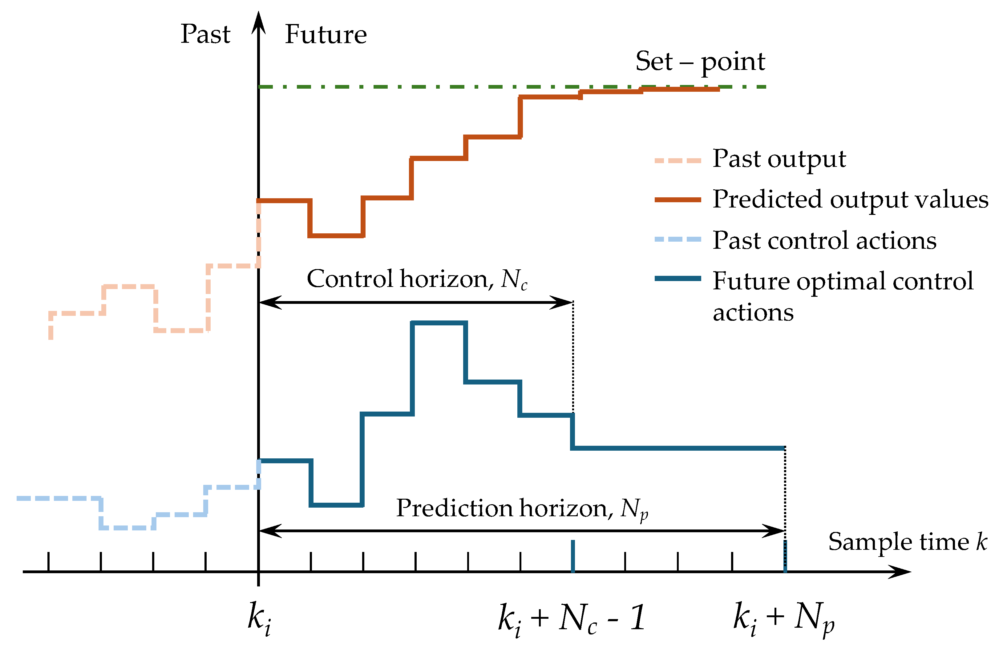
Figure 6.
MPC embedded model and control scheme.
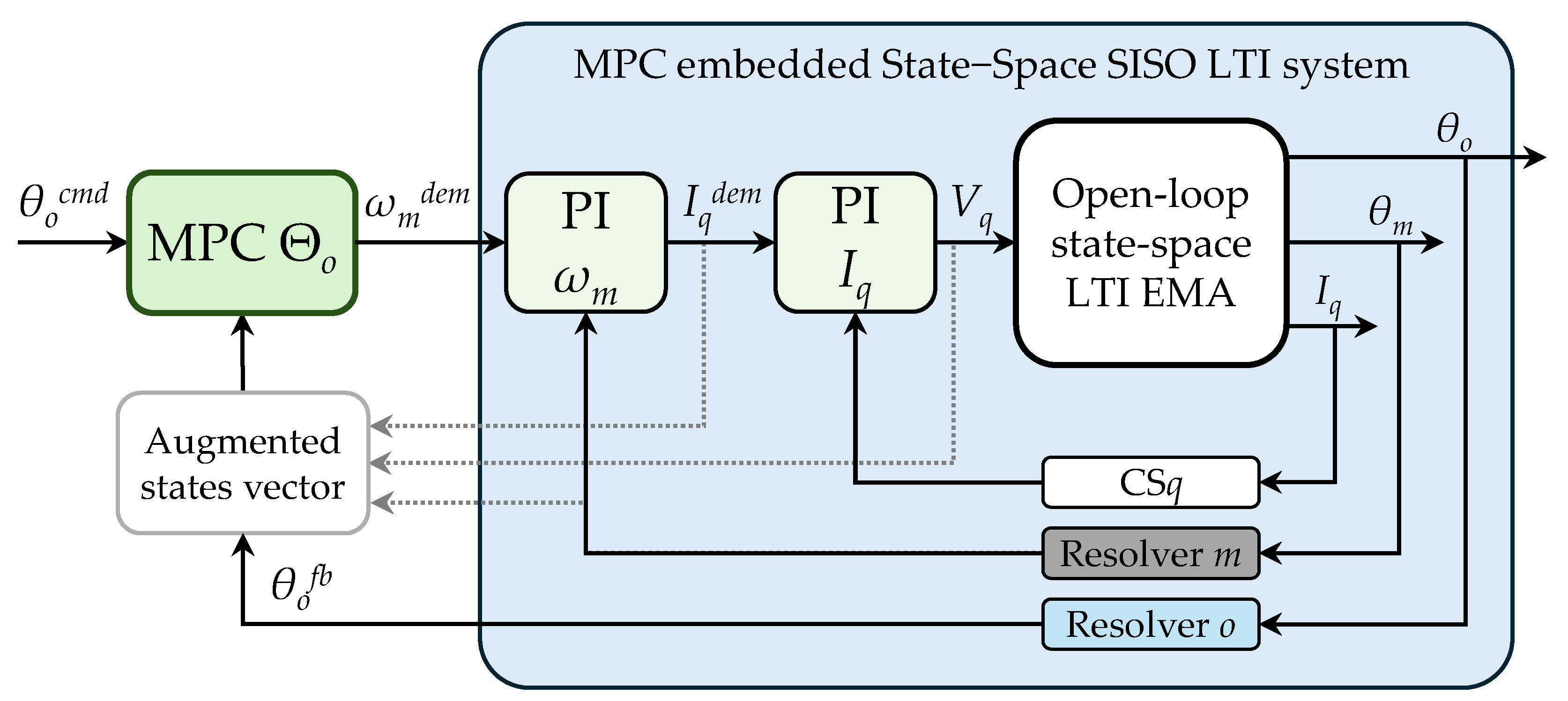
Figure 7.
Gaussian variation of the parameters included in the robustness analysis.
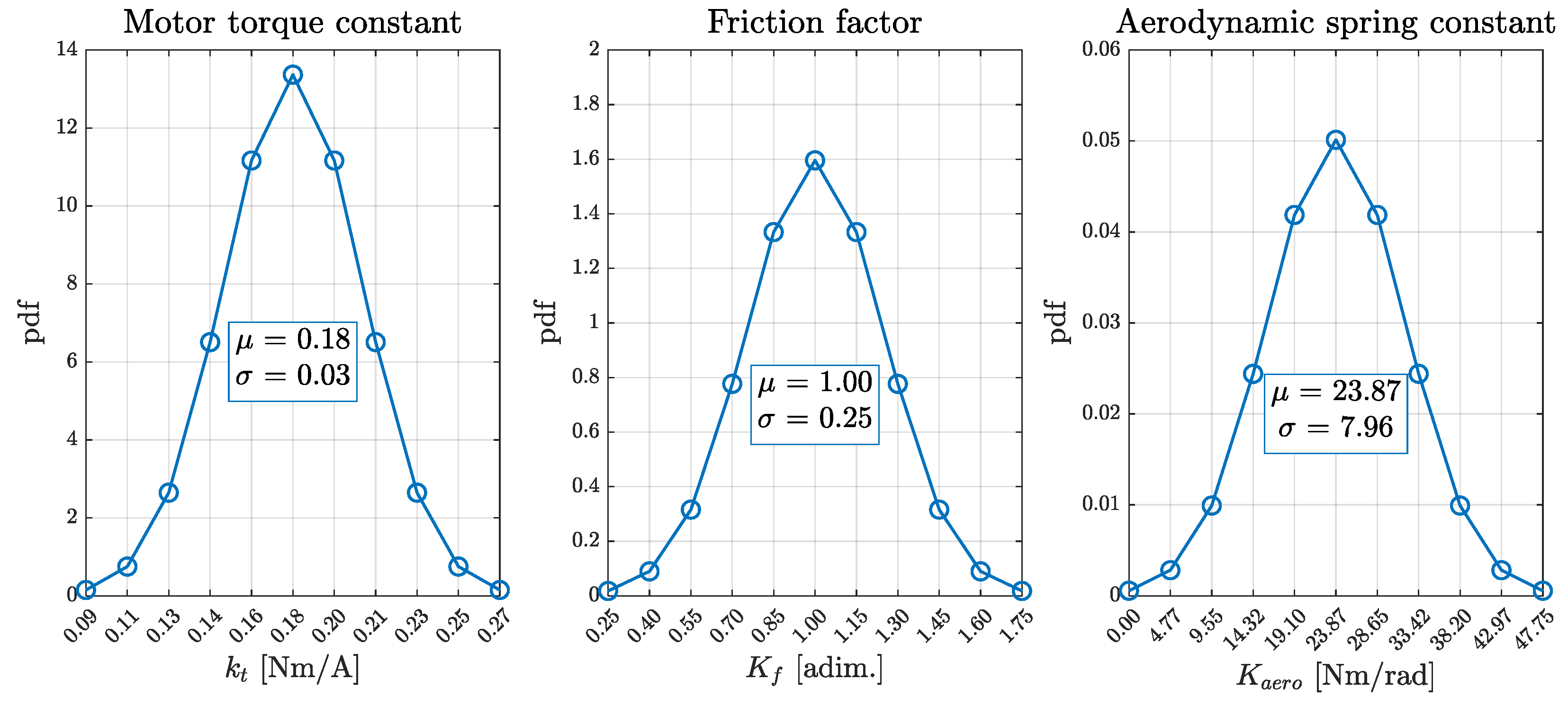
Figure 8.
Cost functions variation with PIs zeros placement.
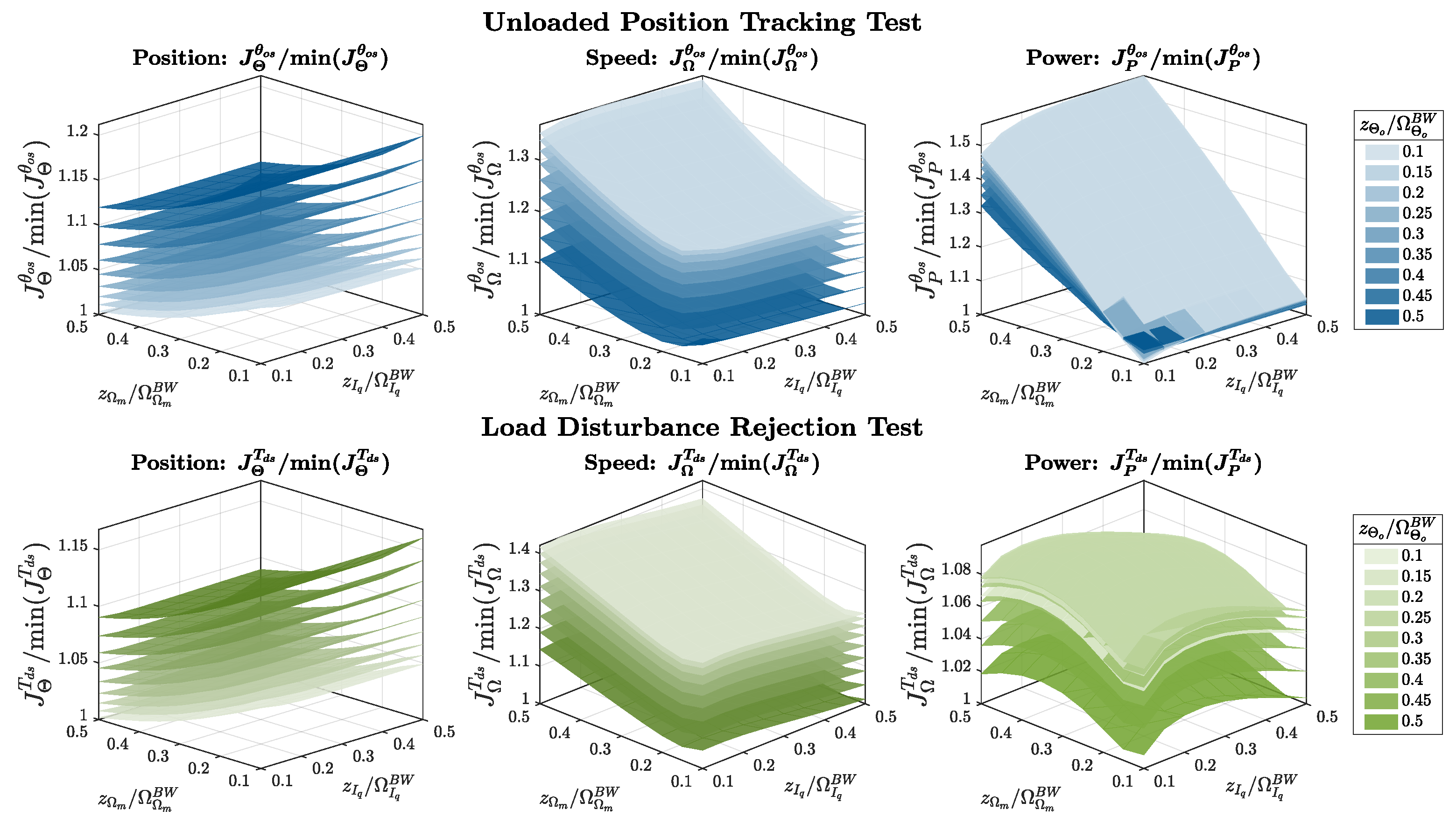
Figure 9.
Normalised cost functions comparison (increasing shade colour with position loop zero).
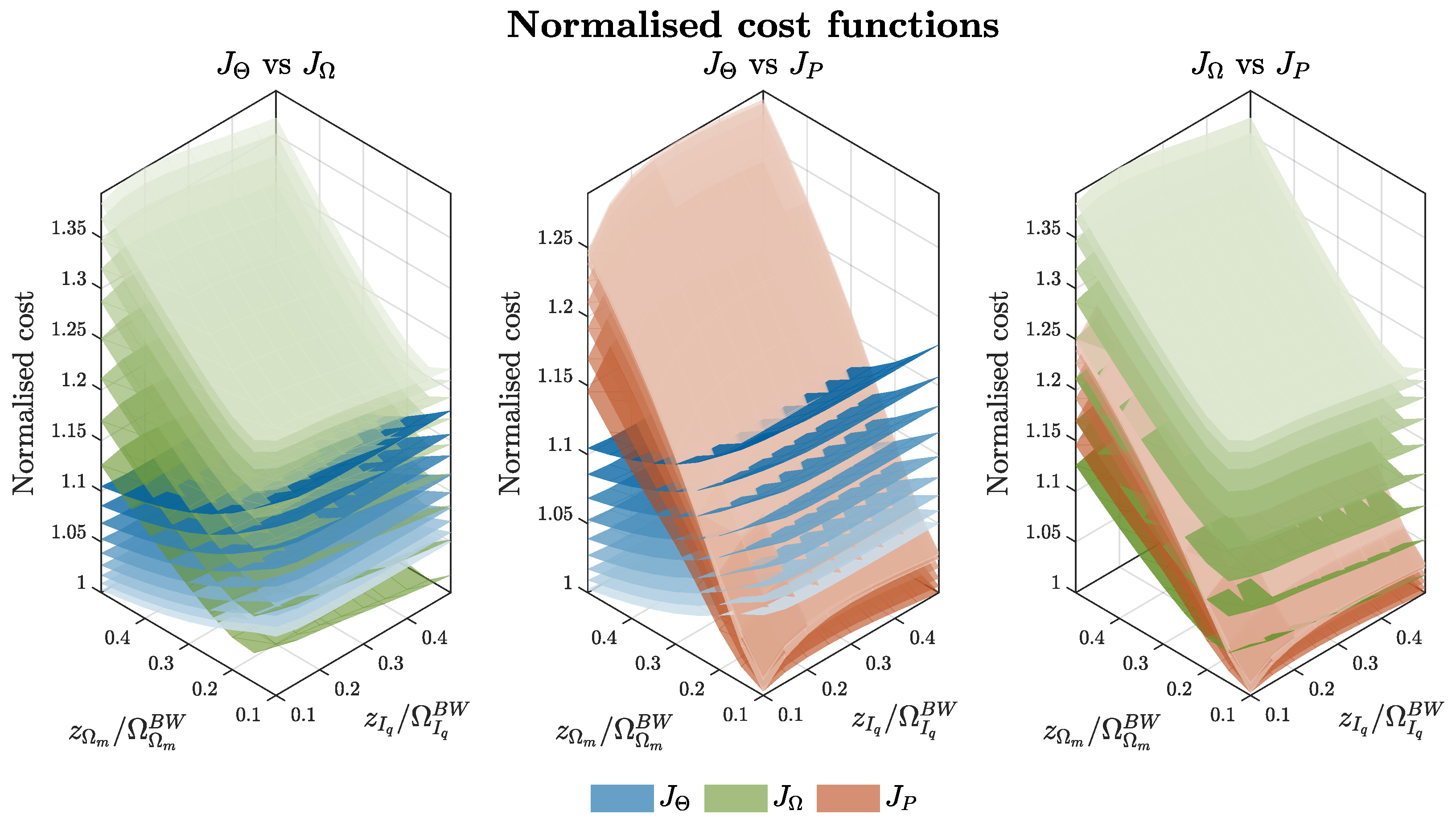
Figure 10.
Global cost function and optimum point.
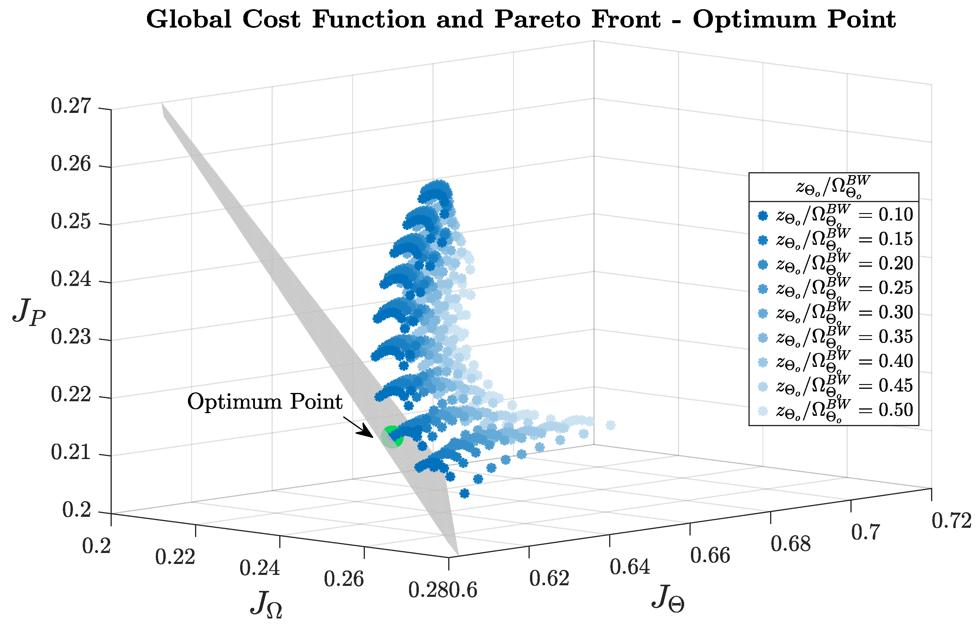
Figure 11.
Unloaded frequency response with 1 deg command amplitude.
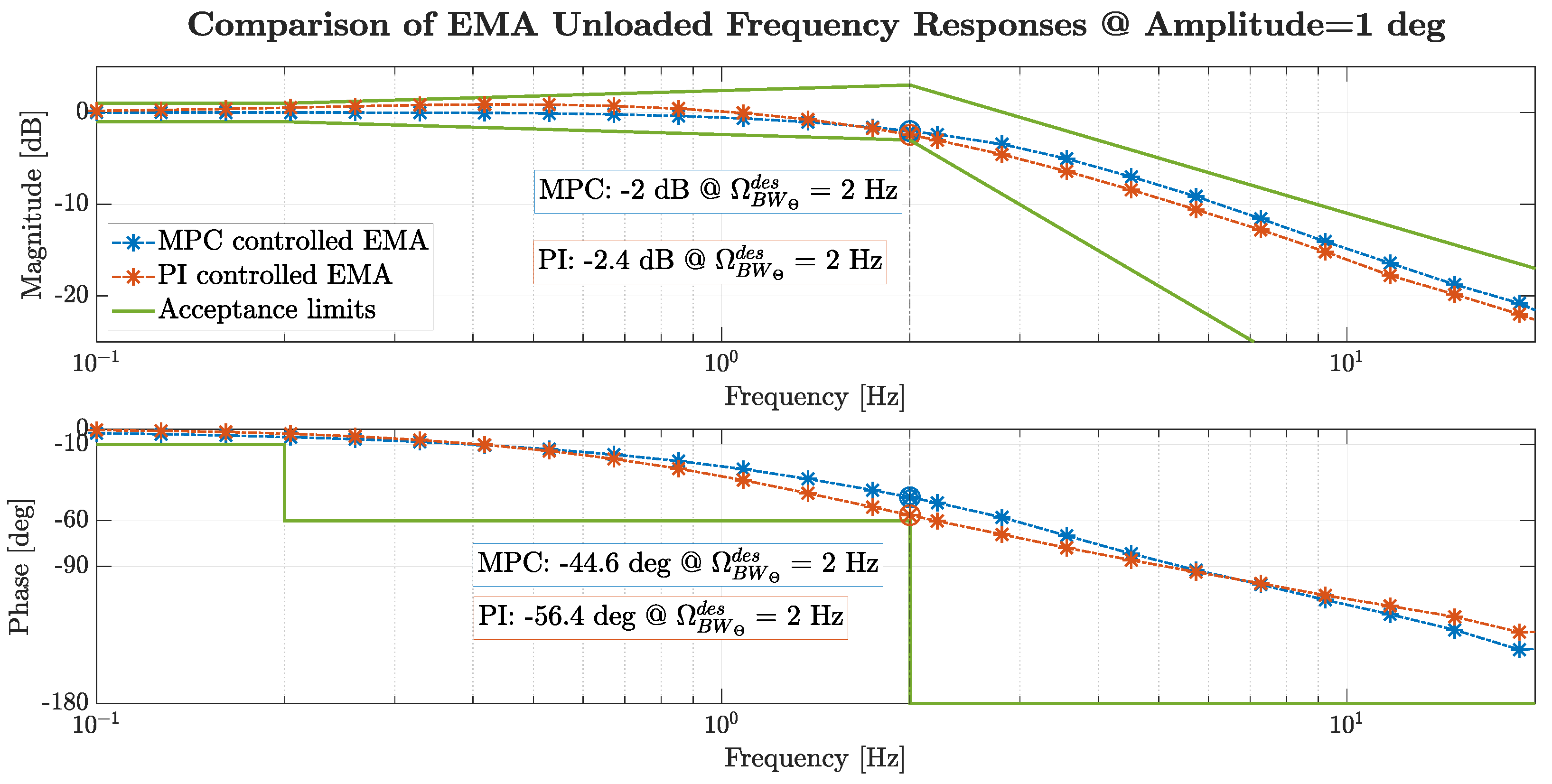
Figure 12.
Frequency response under aerodynamic loads.
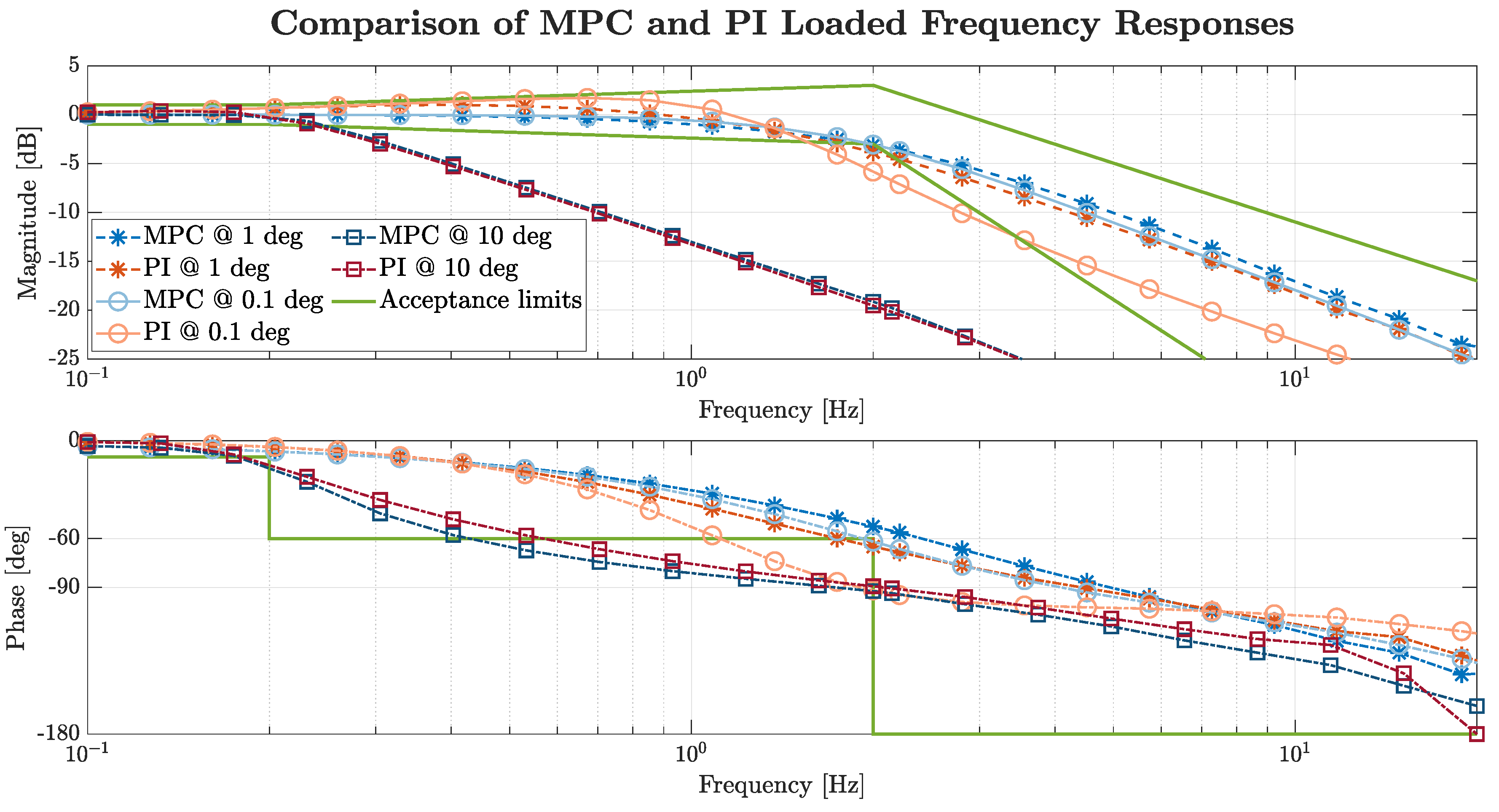
Figure 13.
Rejection to 1 Nm step of external load.
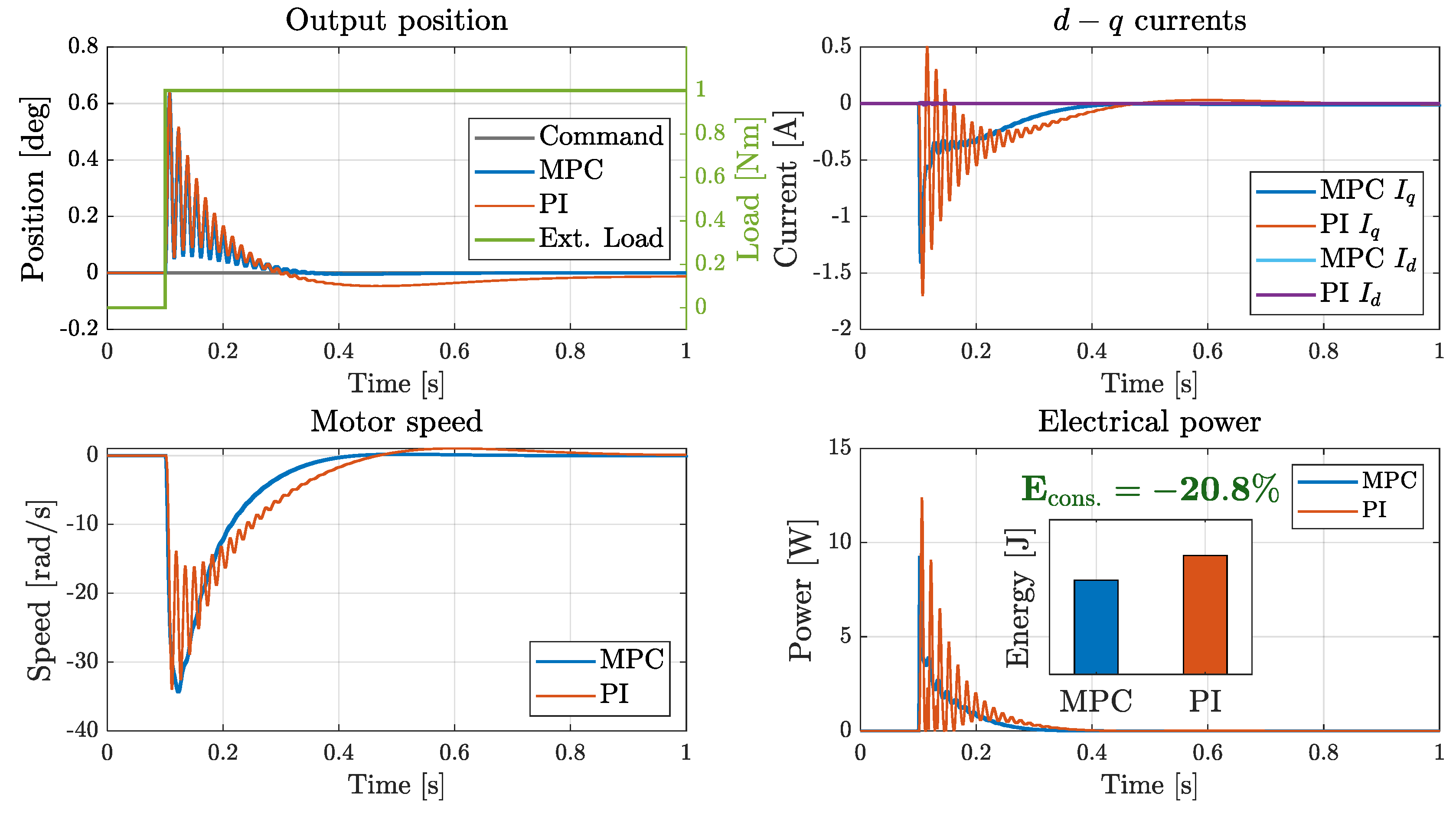
Figure 14.
Dynamic compliance at 1 Nm harmonic load input.
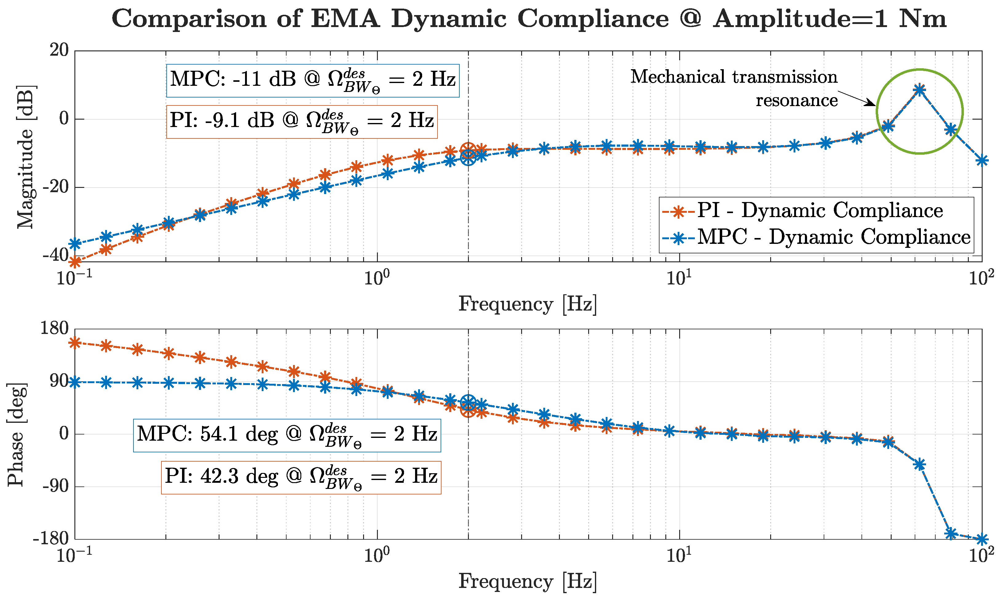
Figure 15.
Motor torque constant effect on MPC- and PI-controlled EMAs.
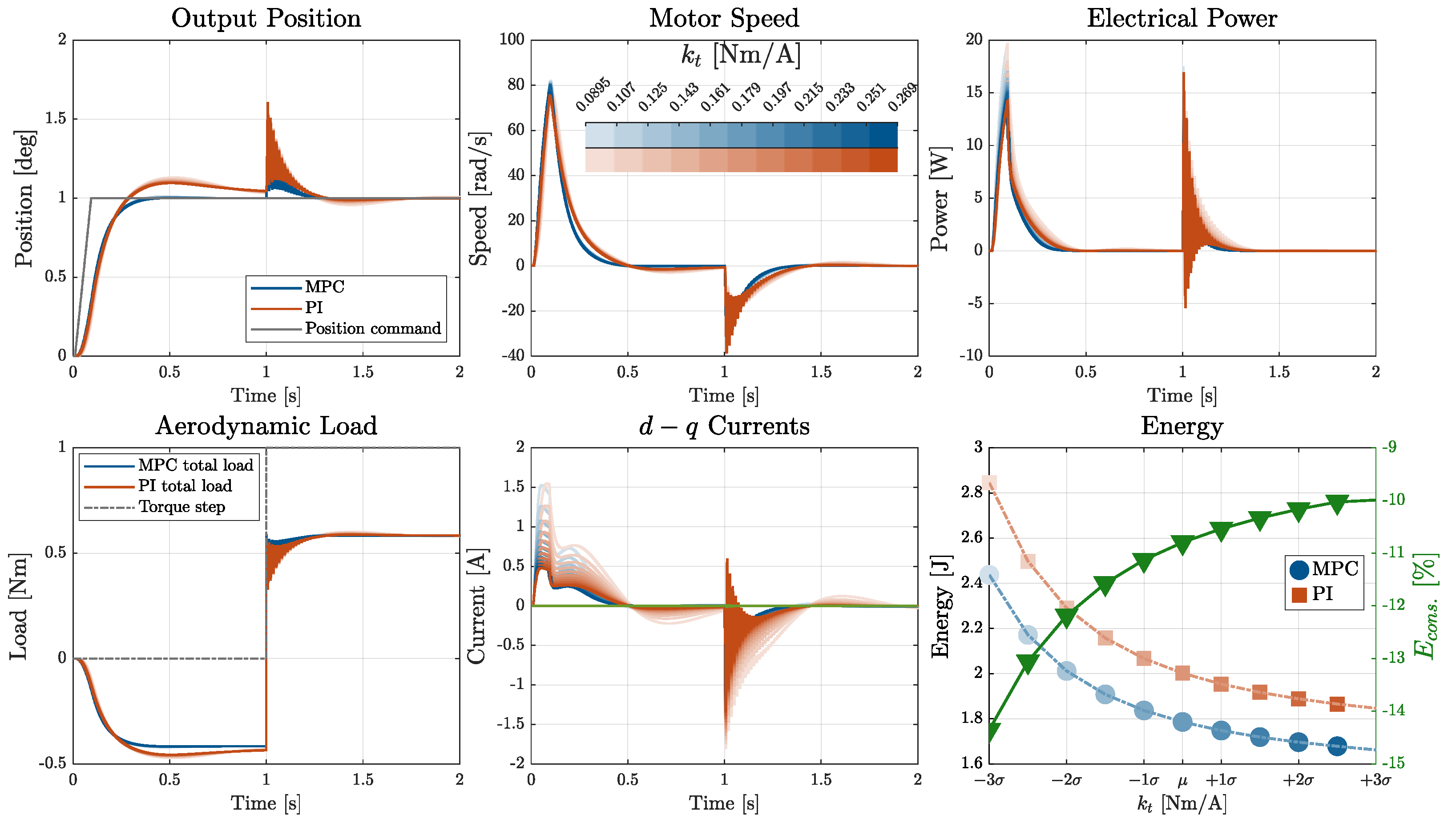
Figure 16.
Friction coefficients multiplier effect on MPC- and PI-controlled EMAs.
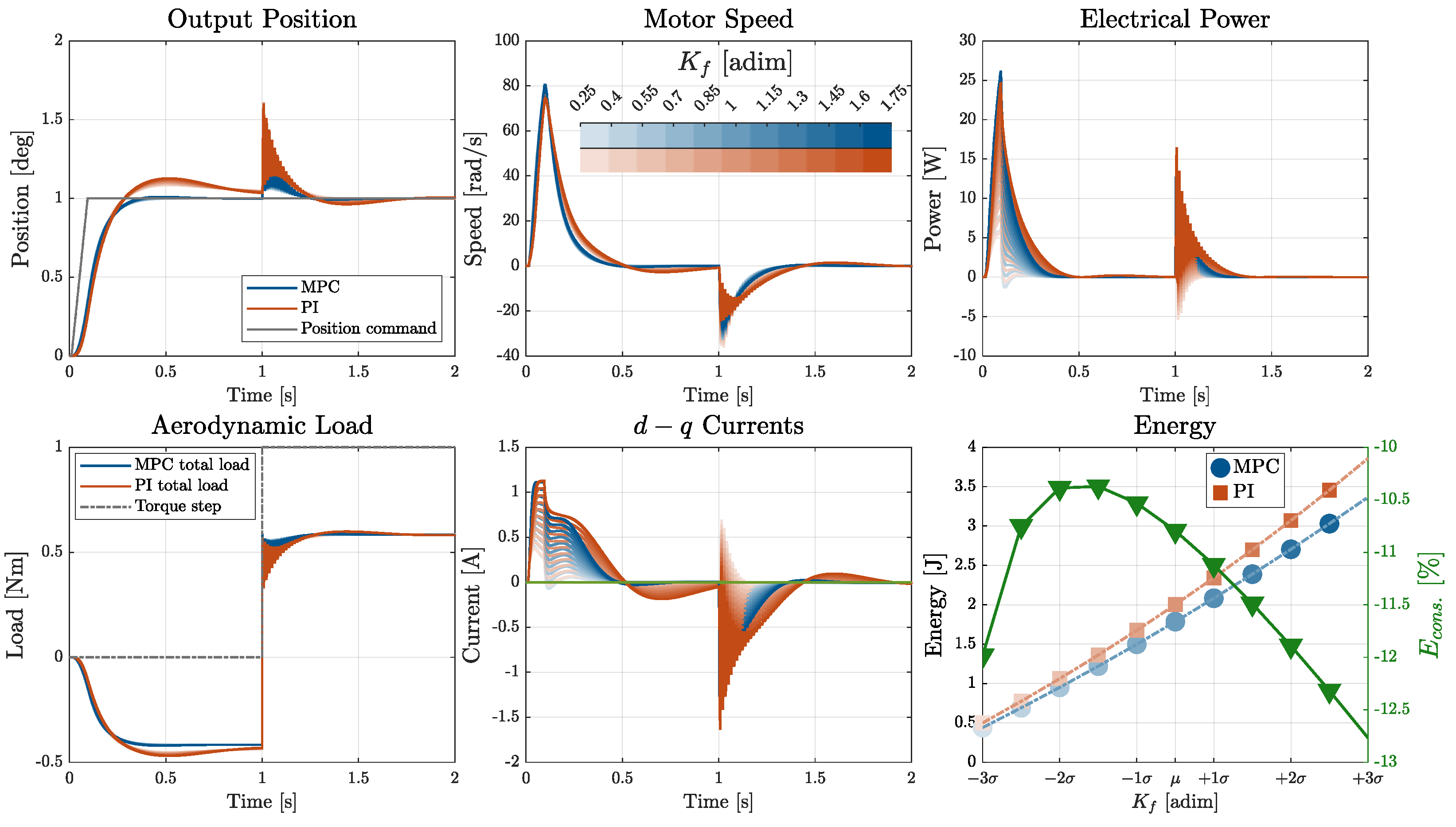
Figure 17.
Aerodynamic spring load stiffness effect on MPC- and PI-controlled EMAs.
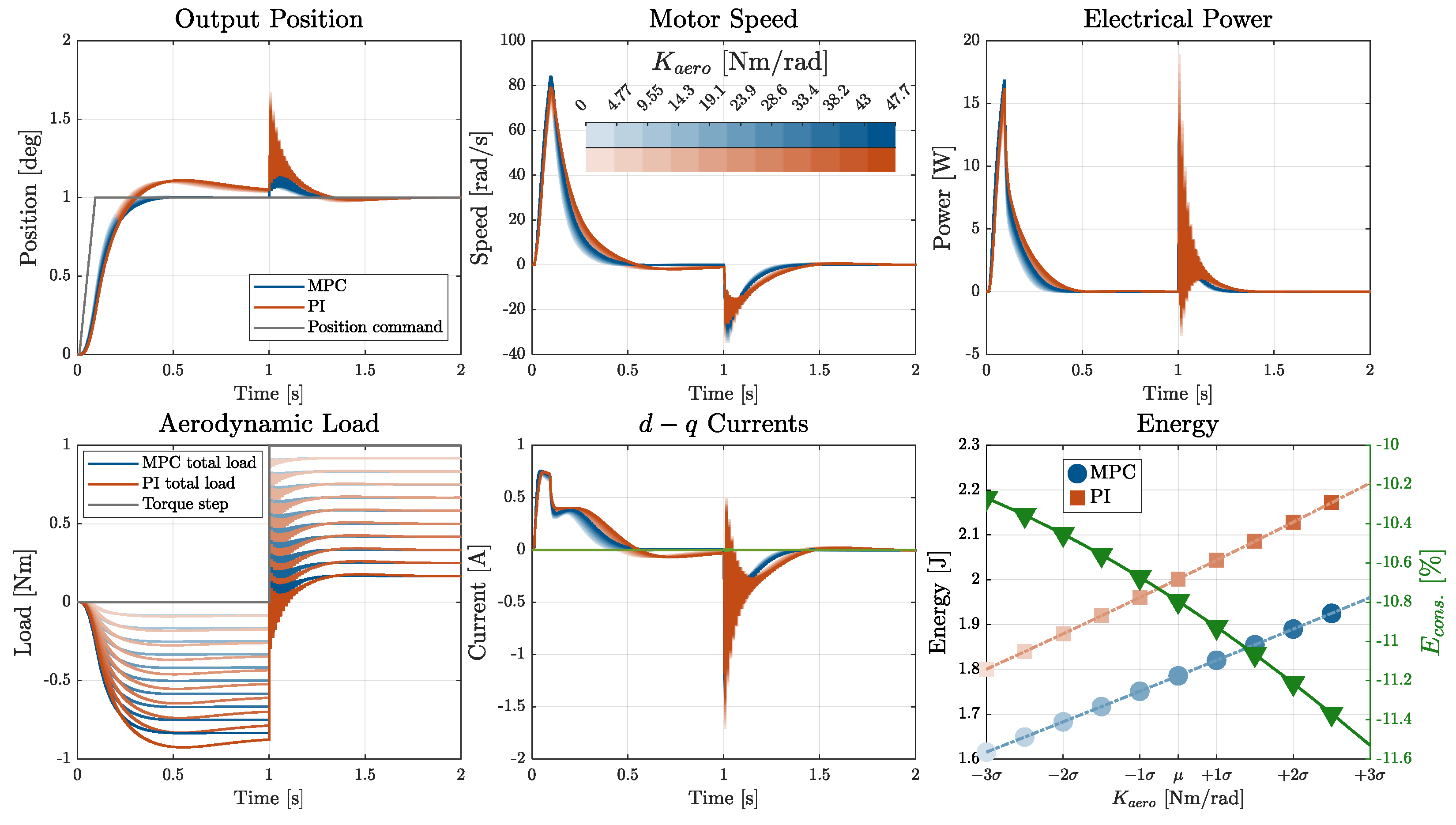
Figure 18.
Statistical metrics of the position error deviation under combined parameters variation.
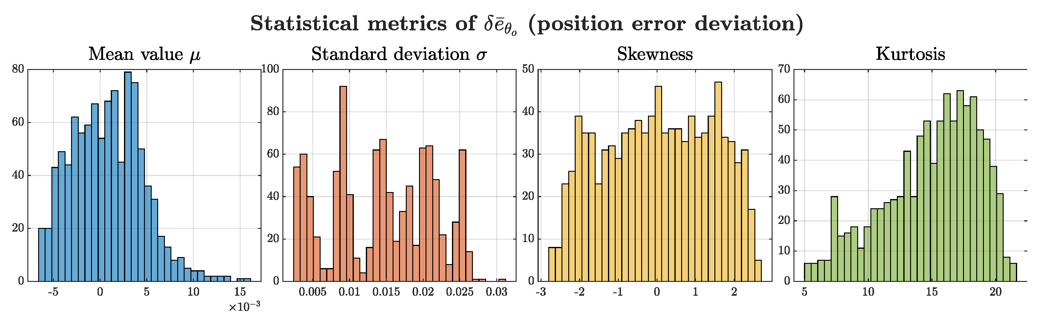
Figure 19.
Dependency of the position error deviation statistical metrics on the three parameters.
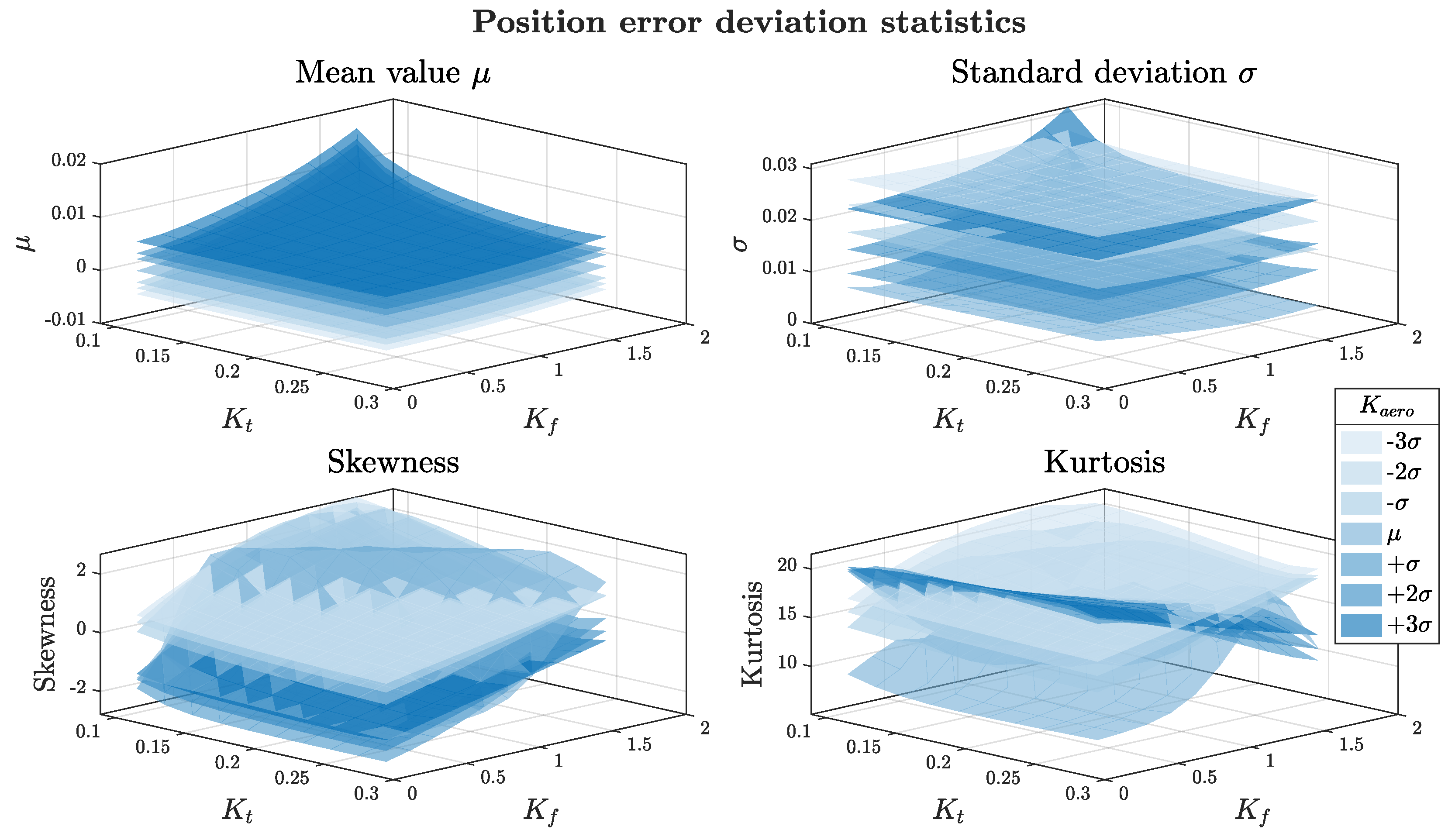
Figure 20.
Statistical metrics of the power consumption deviation under combined parameters variation.
Figure 20.
Statistical metrics of the power consumption deviation under combined parameters variation.
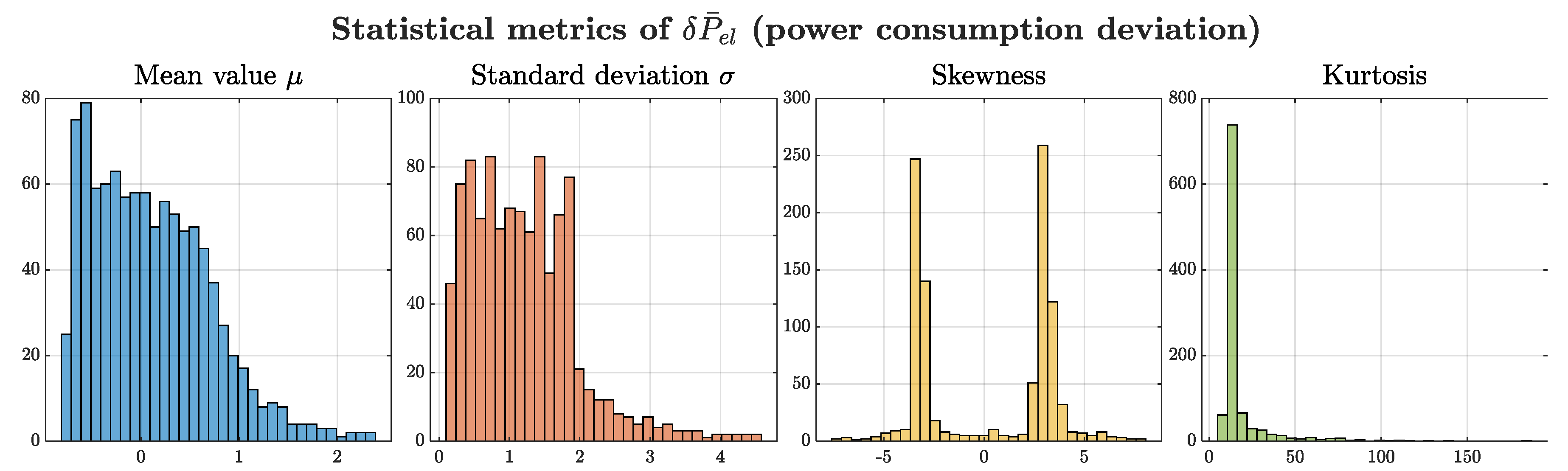
Figure 21.
Dependency of the power deviation statistical metrics on the three parameters.
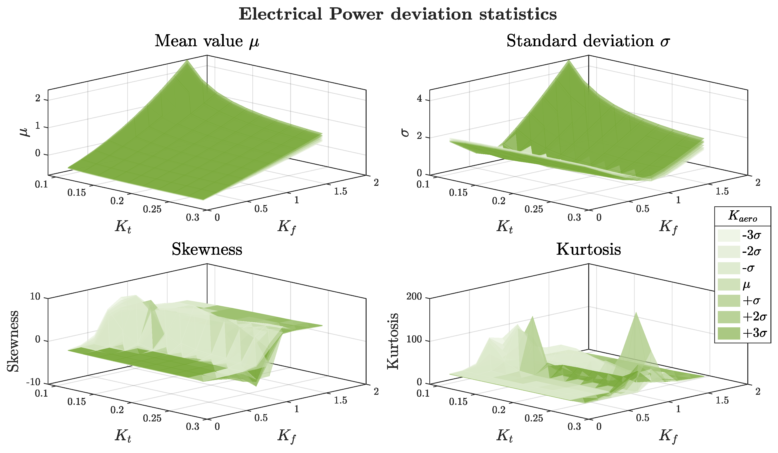

Table 1.
Parameters of the electro-mechanical section.
| Quantity | Meaning | Value | Unit |
|---|---|---|---|
| Jm | Motor shaft inertia | 4⋅10-5 | kgm2 |
| Jo | Output shaft inertia | 1⋅10-3 | kgm2 |
| Kg | Drivetrain torsional stiffness | 166.8 | Nm/rad |
| Cg | Drivetrain torsional damping (I° mode) | 0.0408 | Nms/rad |
| τg | Differential ball-screw gear ratio | 500 | [-] |
| Bm | Viscous friction coefficient | 0.0716 | Nms/rad |
| Tc | Coulomb friction torque | 3.42⋅10-4 | Nm |
| ωc | Coulomb velocity | 10.5 | rad/s |
| Tcmax | Maximum output torque | 25 | Nm |
| θomax | Maximum angular deflection | ±30 | deg |
| ωomax | Maximum output speed | 12 | deg/s |
| ωmmax | Maximum motor speed | 105 | rad/s |
| kt | Motor torque constant | 0.179 | Nm/A |
| Kaeroeq | Equivalent aerodynamic spring stiffness | 23.87 | Nm/rad |
| Iqmax | Maximum quadrature current | 4 | A |
| Rph | Phase resistance | 1.53 | Ω |
| Lph | Phase inductance | 15 | mH |
| nd | Number of pole pairs | 10 | [-] |
| VDCmax | Maximum BUS DC voltage | 36 | V |
Table 2.
Sensors characteristics.
| Sensor type | Bandwidth | Unit |
|---|---|---|
| Resolver (m, o) | 200 | Hz |
| Hall-effect Current sensor (d, q) | 40.000 | Hz |
Table 3.
Control loops design requirements.
| Quantity | Meaning | Current loop | Speed loop | Position loop | Unit |
|---|---|---|---|---|---|
| Ωbw | Bandwidth | 200 · 2π | 20 · 2π | 2 · 2π | rad/s |
| φm | Phase margin | ≥ 45 | ≥ 45 | ≥ 45 | deg |
| Km | Gain margin | ≥ 6 | ≥ 6 | ≥ 6 | dB |
Table 4.
Optimized PI controllers parameters.
| Quantity | Meaning | Value | Unit |
|---|---|---|---|
| KIq | Current loop proportional gain | 16.347 | V/A |
| zIq | Current loop integrator zero | 628.318 | rad/s |
| Kω | Motor speed loop proportional gain | 0.0294 | A s/rad |
| zω | Motor speed loop integrator zero | 18.850 | rad/s |
| Kθ | Output position loop proportional gain | 6085.21 | 1/s |
| zθ | Output position loop integrator zero | 1.256 | rad/s |
Disclaimer/Publisher’s Note: The statements, opinions and data contained in all publications are solely those of the individual author(s) and contributor(s) and not of MDPI and/or the editor(s). MDPI and/or the editor(s) disclaim responsibility for any injury to people or property resulting from any ideas, methods, instructions or products referred to in the content. |
© 2025 by the authors. Licensee MDPI, Basel, Switzerland. This article is an open access article distributed under the terms and conditions of the Creative Commons Attribution (CC BY) license (http://creativecommons.org/licenses/by/4.0/).
Copyright: This open access article is published under a Creative Commons CC BY 4.0 license, which permit the free download, distribution, and reuse, provided that the author and preprint are cited in any reuse.


