
Submitted:
04 June 2025
Posted:
05 June 2025
You are already at the latest version
Abstract
This work presents a nonlinear aerodynamic model that describes the dynamics 1 of a coaxial-rotor MAV. We have designed seven control laws based on linear and nonlinear 2 controllers for path following with a coaxial-rotor MAV in the presence of unknown 3 disturbances, such as wind gusts. The linear controllers are the Proportional-Derivative (PD) 4 and the Proportional-Integral-Derivative (PID). The nonlinear techniques are the nested 5 saturation, sliding mode control, second-order sliding mode, high-order sliding mode, and 6 adaptive backstepping. The results are presented after several computer simulations.
Keywords:
coaxial-rotor MAV
; linear control
; nonlinear control
1. Introduction
The coaxial-rotor MAV (Mini Aerial Vehicle) is an unmanned aerial vehicle that has gained significant acceptance in the research area due to the compact structure of its components (fuselage, ailerons, motors, etc.). Another advantage is the wide variety of applications for these unmanned aerial systems. By the side of the research area with the coaxial-rotor MAV, focus is on design control laws, trajectory follow, aerodynamic structure research, materials analysis, etc. The before is necessary to realize applications in the real world as surveillance, target acquisition, area reconnaissance [1,2].
On the other hand, exists some disadvantages in the use of coaxial-rotor MAVs, some of them are that the design of the electronic systems should be small, and satisfy every necessity to achieve a stable flight. Another disadvantage is the aerodynamic structure design, for example, the distance between the top motor and the bottom motor must be sufficient but not too long to avoid the inter-rotor wash interference to obtain a fixed yaw angle and avoid the rotation in the z-axis in a hover flight.
Finally, these coaxial-rotor MAVs are subject to perturbations by wing gusts like other UAVs (Unmanned Aerial Vehicles). Then, there are a lot of areas of research about coaxial-rotor systems.
In the scientific literature is possible to find research about the coaxial-rotor UAVs to resolve some of the disadvantages mentioned before. For example in [3] is applied the fuzzy logic theory with sliding mode methodology to stabilize the longitudinal attitude of a small coaxial-rotor UAV, the control algorithm is designed decoupling the mathematical model of the coaxial-rotor UAV, with this controller design is possible suppress the modelling error and the external interference, the results of [3] are obtained by computer simulations. In [4] are combined the sliding mode control and PID control algorithm to stabilize the attitude of coaxial-rotor aircraft, the use of the two control laws combined is to achieve a steadily fly and keep the hover position, the mathematical model of the coaxial-rotor craft in [4], it is considering the blade element theory to calculated the brandishing motion of the blades, the results of sliding mode with PID control in [4] are presented in experiments. Other works are focused the research about the coaxial-rotor in the aerodynamics and the external forces acting in the coaxial-rotor UAV [5], and even proposed a better aerodynamic structure to carry generic payloads for different civil and agriculture applications, the results are presented in a numerical form by computer [5]. A combinatorial control method based on sliding mode coupled with a PID control is proposed in [6], and the dynamical model is divided in two subsystems, a fully-actuated subsystem and an under-actuated subsystem, the control objective is to control the position and attitude tracking of a coaxial-rotor aircraft, the results are presented in numerical simulations and experiments. In [7] is presented a dynamic observer is presented to deal with the uncertainties and disturbance and design a control law to stabilize a ducted coaxial-rotor UAV.
It is presented in [8] a coaxial-rotor that it is designed to be small like a package and after to launch with other system, and even, it is development a complete nonlinear aerodynamic modelling for the coaxial-rotor UAV, but after it is simplified, the objective in [8], it is the application of a discrete Kalman filter to estimate the aerodynamic coefficients. In [9] is developed a compact coaxial-rotor to be launched with other propulsion system, and even the coaxial-rotor system includes a rotary-wing mechanism to achieve the rotations in roll and pitch angles, the control strategy is a cascade feedback controller, and in the first time was tested in a wind tunnel, and after tested from arbitrarily large attitude angles to demonstrate the control robustness.
In [10] it is presented a coaxial drone, adding in the aerodynamic structure two servo motors to control the roll and pitch angles, and it is developed a nonlinear dynamic model for the six degrees of freedom of the coaxial drone, and a nonlinear control allocation approach is proposed, the results are presented in numerical simulation, and validates in real experiments.
To achieve the control objective of trajectory tracking although the sensor noise, uncertainty in the model parameters, and external perturbations, in [11] it is proposed a nonlinear robust backstepping sliding mode controller to control the attitude and the position of a coaxial-rotor aircraft, the results are presented in numerical and flight experiments. By other side, in [12] it is proposed a control algorithm to stabilize the position and attitude of a coaxial-rotor drone, but without knowing the mathematical model dynamics, to achieve the objective of control in [12] it is proposed an optimal model-free fuzzy controller and estimating the unknown dynamic, the results are presented in numerical simulations.
In this work is develop a mathematical model dynamics that describes the coaxial-rotor MAV, this dynamic model includes the external disturbances by wind gusts, but in the controllers design is not considered such disturbances to analyze the control responses in the path following subject to unknown wind gusts and carry out a comparison between linear and nonlinear controllers. Then, the control laws that do not the known disturbances in this work are the linear controllers Proportional-Derivative (PD), the Proportional-Integral-Derivative (PID), and the nonlinear controllers based on nested saturation, the sliding modes methodologies based on first, second, and high-order.
It must be mentioned that we are proposing an adaptive backstepping control to try with these unknown disturbances, and to achieve a better path following with the coaxial-rotor MAV, and it is the only controller in this work that has considered the unknown disturbances to design an adaptation law based on the euler angles and angular rates for the roll and pitch angles, the before to eliminate or attenuate the unknown disturbances by wind gusts.
Then, this work is organized as follows: Section 2 shows the mathematical aerodynamic model to define the coaxial-rotor MAV; Section 3 presents the linear and nonlinear controllers design. Section 4 shows the simulation results obtained after several tests. Finally, Section 5 presents the discussion and the future work.
2. Coaxial-Rotor MAV Mathematical Model
In this section, it is presented the mathematical model that describes the coaxial-rotor MAV dynamics based on the Newton-Euler formulation [13,14,15,16,17,18]. The Earth’s curvature is not considered due to the coaxial-rotor MAV flying short distances. To obtain the mathematical model, it is consider two coordinates frames and (see Figure 1), knowledge as the inertial fixed frame, and the body frame, respectively. The body frame is fixed, attached to the center of gravity of the coaxial-rotor MAV [19,20]. The general coordinates in the coaxial-rotor MAV are defined as . The coaxial-rotor MAV mathematical model is given by:
with the translation coordinates relatives to the inertial frame , is the gravitational force. The translational velocity is defined by in with respect to . The mass of the coaxial-rotor MAV is represented by m. The forces working in the coaxial-rotor MAV are given by . The Euler angles are defined with , and is the angular velocity in (see Figure 1). The torques working in the coaxial-rotor MAV are [21,22]. We have added to the aerodynamic model a unknown vector of the wind gusts perturbation , and is applied to compensate the units of measurement. The inertial moments matrix is given by . The matrix is defined as [23]
To obtain the orientation of the coaxial-rotor MAV is necessary to define a rotation matrix as :
Then, the Newton-Euler equations in a stable flight (hover flight) for a coaxial-rotor MAV are given by:
with , , , , , .
where are the inertial moments defined in the matrix . The actuator moments are given by are the control inputs to generate the roll, pitch, and yaw angles, respectively. The angular velocities of the motors are defined with and , and the inertia moment of the propellers are given by and . Finally, the aerodynamic moments are in roll angle, in pitch angle, and for yaw angle (see Figure 1).
2.1. Pitch Angle Response
3. Linear and Nonlinear Controllers Design
To follow the desired trajectory with the coaxial-rotor MAV, in this work, the control laws are designed only for the pitch and roll angles; it is considered that the yaw angle is zero (the two brushless motors in the coaxial-rotor MAV work at the same speed). Then, to know which controller presents the better performance in the presence of unknown wind gust perturbations, let us decouple the equations (8)-(9) to obtain pure roll and pitch angles, but considering the unknown wind gust perturbations in the mathematical model. Thus, the equations to define a pure roll angle with perturbations are defined by:
where , is the air density, the velocity in hover flight is defined as V, the aileron area is defined with S, b is the aileron span, and defined the aerodynamic coefficient in roll angle. The same procedure is considered to define the equations for a pure pitch angle with perturbations:
where , is the average aileron length, and is the aerodynamic coefficient in pitch angle. The desired trajectory to follow by the coaxial-rotor MAV is defined as:
where and are the desired position in the x-axis and the y-axis, respectively. is a positive constant value to define the circumference amplitude of the desired trajectory, t is the time, and w. are the desired roll and pitch angle, respectively. To control the altitude of the coaxial-rotor MAV is design a PID controller defined by , with , is the desired altitude, m is the total mass of the coaxial-rotor MAV, g is the gravitational constant.
It should be mentioned that is not considered in the control laws design, the unknown perturbation by wind gusts () to compare the performance and robustness of the controllers in the presence of unknown perturbations. Except in the adaptive backstepping controller, it is proposed a wind gust estimation is proposed to eliminate or reduce the unknown perturbation defined in (14)-(17).
Thus, to design the linear controllers Proportional-Derivative (PD), and Proportional-Integral-Derivative (PID) for the roll angle, let us defined an error , with as the desire roll angle, and defines the actual roll angle in the coaxial-rotor MAV. The PD control law for roll angle is given by [24,25]:
where . The PID controller in pitch and roll angles for the coaxial-rotor MAV is defined as:
with . To design the nested saturation control in the roll angle, it is necessary to perform a linear transformation to transform the system (14)-(15) [26]:
Then,
with , and . Let us define a saturation function with a limit a:
where a is a constant positive value. Then, for the system (14)-(15) with the linear transformation (24) and the saturation function (25), the controller by nested saturation for roll angle to achieve global asymptotic stability is defined as:
The first-order sliding mode control to stabilize the roll angle is defined from a sliding manifold , and deriving the sliding manifold we have . Then, to stabilize the roll angle defined with the system (14)-(15) using the first-order sliding mode control methodology [27,28] is given by:
where are the controller gains, and the sign function is defined as:
For the design of the second-order sliding mode is necessary a first-order robust differentiator, because a real-time derivative is sensitive to noise at the time of performing the derivative action. The robust real-time differentiator [29], and it is given by
with and are real-time estimates of and , respectively. The and are constant values to adjust the estimations. Then, to stabilize the roll angle with the second-order sliding modes [30], the controller obtained is:
where are positive gains to adjust the second-order sliding mode controller. To design the high-order sliding mode, it is necessary to have a second-order robust differentiator [31], and it is given by:
where , , and are real-time estimations of , , and . The constant values to adjust the estimations are defined by . Finally, the high-order sliding mode controller to stabilize the roll angle in the coaxial-rotor MAV is defined by:
with as positive constant values. For the adaptive backstepping control in roll angle, we are considering the complete system (14)-(15), that is, we are consider the unknown perturbation () to design the adaptation law, and estimating to reduced or eliminated the external perturbations in the coaxial-rotor MAV. Then, the error in roll angle is defined as , and to begin with the adaptive control design, it is defined a Lyapunov candidate function is defined as:
Deriving (35):
The new error is , where . Then, the derivative of (35) is , due to the second term of the is not negative definite, and to continue with the design of the adaptive controller, we have to define a new Lyapunov candidate function given by:
where are the adaptation gains, which are definite positive constants. Then, deriving (38):
Deriving the error :
Considering (39)-(41), the adaptive control law is given by:
Thus,
with . The adaptation equation for the perturbations by wind gusts is given by:
The adaptation gain is defined by . Finally, the equation (52) is negative definite, and it is considering bounded (53), it is possible to achieve definite global stability with the adaptive control law (51) for the system (14)-(15), which defines the roll angle in the coaxial-rotor MAV.
To control the pitch angle are used the same methodologies presented above are used, but applied to the system (16)-(17). Thus, the pitch error for pitch is given by , with as the desired pitch angle, and defines the actual pitch angle. Thus, the linear controller PD and PID are given by:
where are positive definite gains, In the Appendix A and Appendix B are presented the stability proofs in the pitch angle for the PD and PID control laws, respectively. The nested saturation control for pitch angle is developed with the methodology presented in the equations (22)-(25). Thus, the nested saturation control to stabilize the pitch angle is given by:
To achieve the desired pitch angle with the first-order sliding mode control (SMC), it is defined a sliding manifold is defined as . Then, follow the methodology used for roll angle and SMC. The first-order sliding mode for pitch angle is defined as:
where are positive values to tune in the controller. To design the second-order sliding mode is used the same structure of the robust differentiator (28)-(29) is used to obtain and , respectively. Thus, the second-order sliding mode control applied to the pitch angle is given by:
with the controller gains as . Finally, to design the high order sliding mode controller to stabilize the pitch angle in the coaxial-rotor MAV is defined is used the same robust differentiator defined in (31)-(33) to obtain , , and , respectively:
where are positive constant. To design the adaptive backstepping law in pitch angle [32,33,34], it is necessary to follow the methodology presented from (35) to (53). Let us define the adaptive control law in pitch angle as:
Then, the final derivative of the Lyapunov candidate function in pitch angle is:
where are positive definite gains to tune the adaptive controller. The adaptation equation for the perturbations by wing gusts is given by:
with as the adaptation gain for the pitch angle.
4. Simulation Results
To do the comparison between the linear and nonlinear control laws, we have used the to know the error of every controller applied to the coaxial-rotor MAV. The for the error is defined as:
The same is applied to calculate the control effort of each control law, and it is defined as:
represents the roll and pitch angles in the coaxial-rotor MAV, respectively.
4.1. Roll Angle Response
The Figure 2, it is presented the roll angle response is presented with the different linear and nonlinear controllers. We can see oscillations due to the external perturbation (wind gusts). The PD, PID, and nested saturation controllers have presented more oscillations, but the perturbations in these control laws are oscillating on the desired roll angle to achieve the desired trajectory with the coaxial-rotor MAV. On the other hand, the nonlinear controllers based on sliding modes methodologies and adaptive backstepping have presented a better performance than PD, PID, and the nested saturation control in the presence of disturbances.
In the same Figure 2, it is appreciated that the sliding mode methodologies achieve the desired roll angle, but the second-order sliding mode (2SM) and high-order sliding mode (HOSM) achieve the desired roll angle with an overdamped signal form. On the other hand, we can see that the first-order sliding mode (SM) and the adaptive backstepping presented a critically damped signal form to achieve the desired roll angle.
The controller that presented a small error in roll angle is the adaptive backstepping, and the big error presented with the second-order sliding mode control (2SM), see Table 1.
Analysing the control effort in the Table 1, the first-order sliding mode control (SM) presented a big control effort to achieve the control objective in the roll angle, and presented a bigger chattering effect in comparison with the second-sliding mode control (2SM), and the high-order sliding mode (HOSM), see the Figure 6, Figure 7 and Figure 8. The PD and PID controllers applied a smaller control effort in comparison with the other control techniques in roll angle, but the adaptive backstepping is close to the control effort values presented with the PD and PID controllers, see Table 1.
4.2. Pitch Angle Response
The pitch angle responses with the linear and nonlinear controllers are presented in Figure 10. The linear controllers PD and PID presented oscillations on the desired pitch angle, and the same signal is presented by the nested saturation control, which before due to the wind gusts. The second-order sliding mode (2SM) achieves the desired pitch angle as an overdamped signal. The first-order sliding mode control (SM), adaptive backstepping technique, and the high-order sliding mode (HOSM) achieve the desired pitch angle as a critically damped signal, see the Figure 10.
The control law with a small error presented in pitch angle is the adaptive backstepping, it can be appreciated in the Table 2. The big error in pitch angle is presented by the PD control.
The PID control presented a small control effort to achieve the desired pitch angle, and the first-order sliding modes applied a big control effort to achieve the desired pitch angle, see the Table 2. Even more, in the Figure 14, Figure 15 and Figure 16 it is appreciated that the first-order sliding mode control presented the biggest chattering effect in comparison with the second-order sliding mode (2SM) and high-order sliding mode (HOSM) controllers.
4.3. Trajectory Follow by the Coaxial-Rotor MAV
In the Figure 18 and Figure 19 are presented the trajectory followed by the coaxial-rotor MAV and every linear and nonlinear controller in the x-axis and y-axis, respectively. The altitude is affected by the disturbances caused by wind gusts, the before can be seen in Figure 20. Finally, in the Figure 21, it is presented the complete trajectory to follow by the coaxial-rotor MAV.
5. Discussion
In this work it a comparison is presented between seven controllers in path following applied to a coaxial-rotor MAV, such control laws are linear and nonlinear control laws. The linear controllers are: Proportional-Derivative (PD) and Proportional-Integral-Derivative (PID). The nonlinear controllers are nested saturation, the sliding modes methodologies based on first, second, and high-order, and the adaptive backstepping technique.
The control laws were designed to path following through stabilizing the roll and pitch angles, the yaw angle, it is considered that the motors are working at the same velocity, in consequence the yaw angle is no changing during the path following, and the altitude control in the coaxial-rotor MAV was achieved with a PID control.
In roll angle, the PID control at the first twenty seconds presented an initial overshoot bigger than the nested saturation control and after twenty seconds persists some oscillations due to the disturbances by wind gusts, the PD control in roll angle presented oscillations too, but the nested saturation control presented a small oscillations in magnitude, in comparison with the PD and PID control (the same signal responses are obtained in the pitch angle). The three methodologies based on sliding modes in the roll angle achieved to desired roll angle in an overdamped signal form, and the controllers based on sliding mode presented an acceptable response in presence of the unknown disturbances, but the control signal has presented the undesired chattering effect, and the chattering effect was reduced but not eliminated by the high-order sliding mode control in the roll angle (it is presented the same effect in pitch angle).
The adaptive backstepping achieved to desired roll and pitch angles in a critically damped signal form, but remember that in these controllers an adaptation laws were designed to estimate the disturbances caused by wind gusts. The control laws that presented a smaller error in roll and pitch angles were the adaptive backstepping, and the bigger error in roll and pitch angles was presented by the second-order sliding mode and the PD, respectively. The smaller control effort in roll angle was presented by the PD and PID, but the smaller control effort signal in pitch angle was presented by the PID control, and the bigger control effort in roll and pitch angles was presented with the first-order sliding mode control.
In conclusion for this work the better response in path following with the coaxial-rotor MAV was achieved by the adaptive backstepping control, because the adaptive backstepping technique presented the smaller error for the control objective in roll and pitch angles, and even, the adaptive backstepping has applied only more of control effort signal than the PD and PID controllers.
The future work consists of finishing the coaxial-rotor MAV to carry out experiments and probe in real flights the seven control laws developed in this work, and to demonstrate the stability proof for the nested saturation control and the sliding modes methodologies.
Author Contributions
Conceptualization, T. and A.; methodology, T.; software, I.; validation, T., A. and I.; formal analysis, J.; investigation, T.; resources, I., and A.; data curation, A., and J.; writing—original draft preparation, T.; writing-review and editing, A., I.; visualization, A.; supervision, T., J.; project administration, T.; funding acquisition, T., A., and I. All authors have read and agreed to the published version of the manuscript.
Funding
Not applicable.
Institutional Review Board Statement
Not applicable.
Informed Consent Statement
Not applicable.
Data Availability Statement
Data available on request due to restrictions.
Conflicts of Interest
The authors declare no conflict of interest.
Abbreviations
The following abbreviations are used in this manuscript:
| MAV | Mini Aerial Vehicle |
| DOF | Degrees of Freedom |
| SO(3) | Special Orthogonal Group in 3D |
| PD | Proportional-Derivative |
| PID | Proportional-Integral-Derivative |
| SMC | Sliding Mode Control |
| 2SM | Second-order Sliding Mode |
| HOSM | High Order Sliding Mode |
Appendix A
In this appendix is presented the PD stability proof in the pitch angle, the same methodology is used for the roll angle with PID controller, but in this work, it is only presented for pitch angle to avoid redundancies or repetitions in the writing. Be , the variable state of the pitch angle system. The dynamic of the system is defined as:
where , . Be the signal reference. It is defined the pitch angle error as:
There is a control objective in the regulation such that:
For this purpose, the following control law is proposed.
where , is the proportional action gain and the derivative action gain, respectively.
Theorem A.1.
The system can be regulated (A10) for a value of , by applying a control law in (A4) which guarantees global asymptotic stability with , .
Proof. The system (A10) is rewritten in terms of the error as follows:
The closed loop system (A5) presents a single equilibrium point in , . Since the equilibrium is located outside the origin, the following change of variable is proposed to move it to the origin:
Substituting (A6) in (A5) Now the system can be written as:
The equilibrium point of (A7) now it is , . To demonstrate stability in the Lyapunov sense, the following candidate function is proposed, which is positive definite and radially unbounded:
The derivative along the trajectories of (A8) is:
It can be observed that . Having a positive definite and radially unbounded FCL, a derivative along the negative semidefinite trajectories, and the fact that the only equilibrium point is the origin, we can conclude the global asymptotic stability of the origin by employing the LaSalle Invariance Theorem. □
Appendix B
In this appendix is presented the PID stability proof in the pitch angle, the same methodology is used for the roll angle with PID controller, but in this work, it is only presented for pitch angle to avoid redundancies or repetitions in the writing. Be , the states of the system.
The system dynamic response is given by:
where , . Be the reference signal, the error is defined as:
There is a control objective in the regulation such that:
For this purpose, the following control law is proposed.
where , , are the proportional, derivative and integral gains, respectively.
Theorem 2.
Proof. The system (A1) is rewritten in terms of the error and as follows:
The closed loop system (A14) presents a single equilibrium point in , ,. Since the equilibrium is located outside the origin, the following change of variable is proposed to move it to the origin:
Substituting (A15) in (A14) Now the system can be written as:
The equilibrium point of (A16) now is , , . To demonstrate stability, the direct Lyapunov method for linear systems will be used. The following Lyapunov candidate function is proposed:
with
The matrix P It is symmetric and positive definite (i.e. ) to ensure that the function is positively definite and radially unbounded. The derivative along the trajectories of (A17) is:
where
It is sought that . Choosing P with the following form:
and respecting the following dimensions for , and :
An asymptotic stability of the origin can be guaranteed. □
References
- Prior S.; Bell C. Empirical Measurements of Small Aerial Co-Axial Rotor Systems, Journal of Science and Innovation, Vol. 1, Issue. 1 pp. 1-18, 2011.
- Ramesh P.; Jeyan J. Hover Performance Analysis of Coaxial Mini Unmanned Aerial Vehicle for Applications in Mountain Terrain, Vilnius Gediminas Technical University-Aviation, Vol. 26, Issue. 2 pp. 1-12, 2022.
- Li K.; Wei Y.; Wang W.; Deng H. Longitudinal Attitude Control Decoupling Algorithm Based on the Fuzzy Sliding Mode of a Coaxial-Rotor UAV, MDPI Electronics, Vol. 8, Issue. 1 pp. 1-16, 2019.
- Wei Y.; Chen H.; Li K.; Deng H.; Li D. Research on the Control Algorithm of Coaxial Rotor Aircraft based on Sliding Mode and PID, MDPI Electronics, Vol. 8, Issue. 12 pp. 1-19, 2019.
- Singh V.; Kanani A.; Panchal N.; Mathur H. Dynamic Analysis of Coaxial Rotor Systems, International Journal of Mechanical and Production Engineering Research and Development, Vol. 10, Issue. 3 pp. 1-13, 2020.
- Wei Y.; Deng H.; Pan Z.; Li k.; Chen H. Research on a Combinatorial Control Method for Coaxial Rotor Aircraft Based on Sliding Mode, Elsevier Defence Technology, Vol. 18, pp. 280-292, 2022.
- Xu C.; Su C. Dynamic Observer-based H-infinity Robust Control for a Ducted Coaxial-rotor UAV, IET Control Theory and Applications, Vol. 16, pp. 1165-1181, 2022.
- Koehl A.; Rafaralahy H.; Boutayeb M.; Martinez B. Aerodynamic Modelling and Experimental Identification of a Coaxial-Rotor UAV, Journal of Intelligent and Robotic Systems, Vol. 68, pp. 53-68, 2020.
- Denton H.; Benedict M.; Kang H. Design, development, and flight testing of a tube-launched coaxial-rotor based micro air vehicle, International Journal of Micro Air Vehicles, Vol. 14, pp. 1-12, 2022.
- Chen L.; Xiao J.; Zheng Y.; Alagappan N.; Feroskhan M. Design, Modeling, and Control of a Coaxial Drone, IEEE Transactions on Robotics, Vol. 40, pp. 1650-1663, 2024.
- Xu J.; Hao Y.; Wang J.; Li L. The Control Algorithm and Experimentation of Coaxial Rotor Aircraft Trajectory Tracking Based on Backstepping Sliding Mode, MDPI Aerospace, Vol. 8, Issue. 11 pp. 1-17, 2021.
- Glida H.; Chelihi A.; Abdou L.; Sentouh C.; Perozzi G. Trajectory Tracking Control of a Coaxial Rotor Drone: Time-delay Estimation-based Optimal Model-free Fuzzy Logic Approach, ISA Transactions, Vol. 137, pp. 1-13, 2023.
- Goldstein H.; Poole C.; and Safko J. Classical Mechanics, Adison-Wesley, USA, 1983.
- Castillo P.; Lozano R.; Dzul A. Modelling and Control of Mini-Flying Machines, Ed. Springer, London, 2005.
- Garcia L.; Dzul A.; Lozano R.; Pégard A. Quad Rotorcraft Control:Vision-Based Hovering and Navigation, Ed. Springer-Verlag, London, 2013.
- O’Reilly O.M. Intermediate Dynamics for Engineers, Ed. Cambridge University Press, UK, 2020.
- Ardema M.D. Newton-Euler Dynamics, Ed. Springer, USA, 2005.
- Craig J.J. Introduction to Robotics Mechanics and Control, Ed. Pearson Education International, third edition, USA, 2005.
- Stengel R. F. Flight Dynamics, Princeton University Press, USA, 2004.
- Cook M. Flight Dynamics Principles, Ed. Elsevier,Second edition, 2007.
- Stevens B.; Lewis F.; Johnson E. Aircraft Control and Simulation, Ed. Jhon Wiley and Sons, third edition, USA, 2015.
- Mclean D. Automatic Flight Control Systems, Ed. Prentice hall International, USA, 1990.
- Espinoza-Fraire T.; Dzul A.; Parada R.; Sáenz A. Design of Control Laws and State Observers for Fixed-WIng UAVs: Simulation and Experimental Approaches, Ed. Elsevier, UK, 2023.
- Kelly R.; Santibañez V.; Loría L. Control of Robot Manipulators in Joint Space, Ed. Springer, USA, 2005.
- Ogata K. Modern Control Engineering, Ed. Prentice Hall, Fifth edition, New Jersey, 2009.
- Teel A. Global stabilization and restricted tracking for multiple integrators with bounded controls, Systems and Control Letters, Vol. 18, Issue 3, pp. 165-171, 1992.
- Khalil H. Nonlinear Systems, Prentice Hall, third Edition, USA, 1995.
- Shtessel Y.; Edwards C.; Fridman L.; Levant A.; Sliding Mode Control and Observation, Birkhäuser, New York, 2015.
- Levant A. Robust exact differentition via sliding mode technique, Automatica, Vol. 34, Issue 3, pp. 379-384, 1998.
- Levant A. Construction principles of 2-sliding mode design, Automatica, Vol. 43, Issue 4, pp. 576-586, 2007.
- Levant A. Higher-order sliding modes, differentiation and output-feedback control, International Journal of Control, Vol. 76, Issue 9-10, pp. 924-941 , 2003.
- Åström K.; Wittenmark B. Adaptive Control, Ed. Prentice Hall, 2nd Edition, 1994.
- Kristić M.; Kanellakopoulos I.; Kokotović P. Nonlinear and Adaptive Control Design, Ed. John Wiley and Sons, USA, 1995.
- Wang W.; Wen C.; Zhou J. Adaptive Backstepping Control of Uncertain Systems with Actuator Failures, Subsystem Interactions, and Nonsmooth Nonlinearities, Ed. CRC Press, UK, 2017.
Figure 1.
Coordinate systems on the coaxial-rotor MAV.
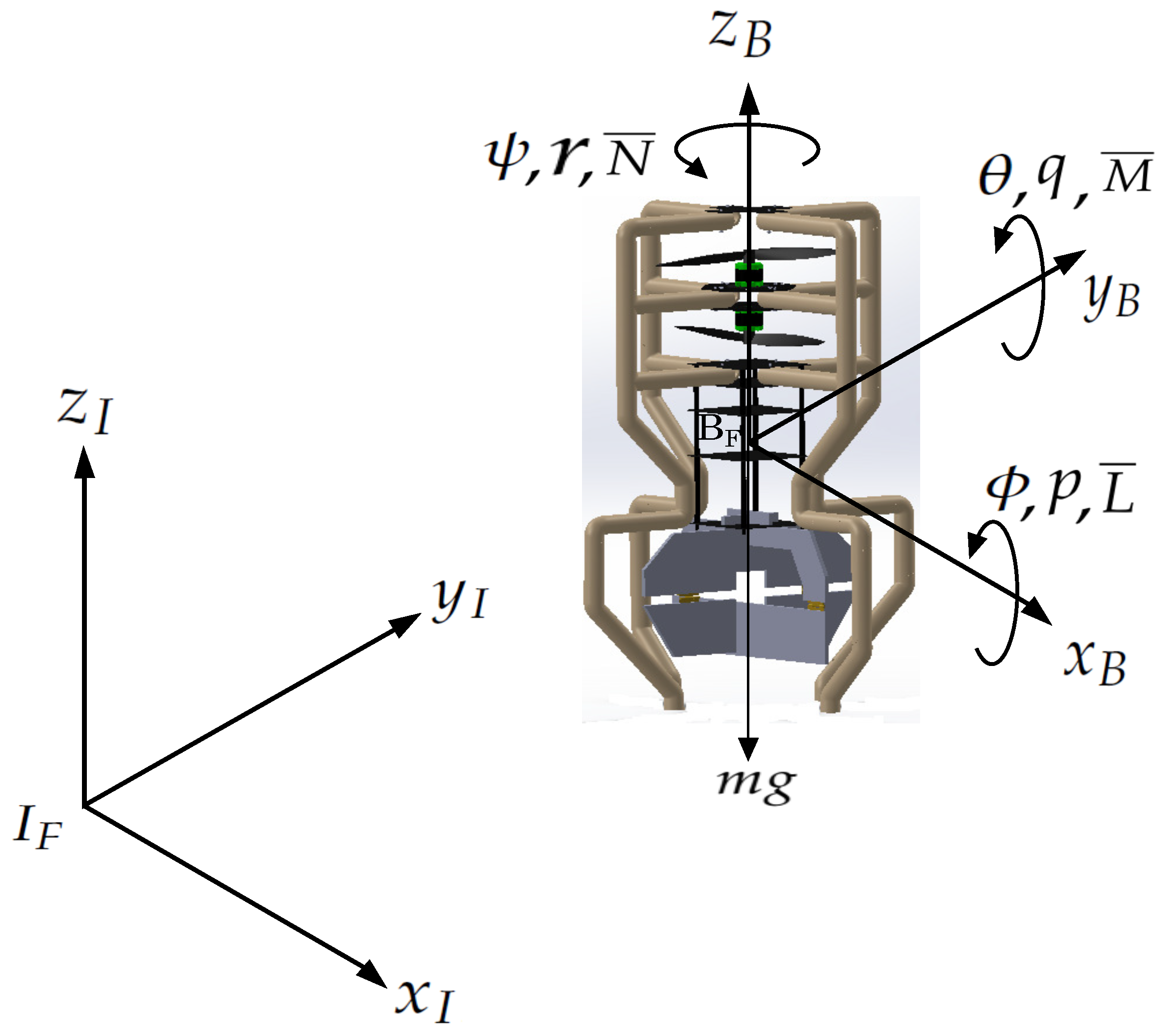
Figure 2.
Response in roll angle (with disturbances).
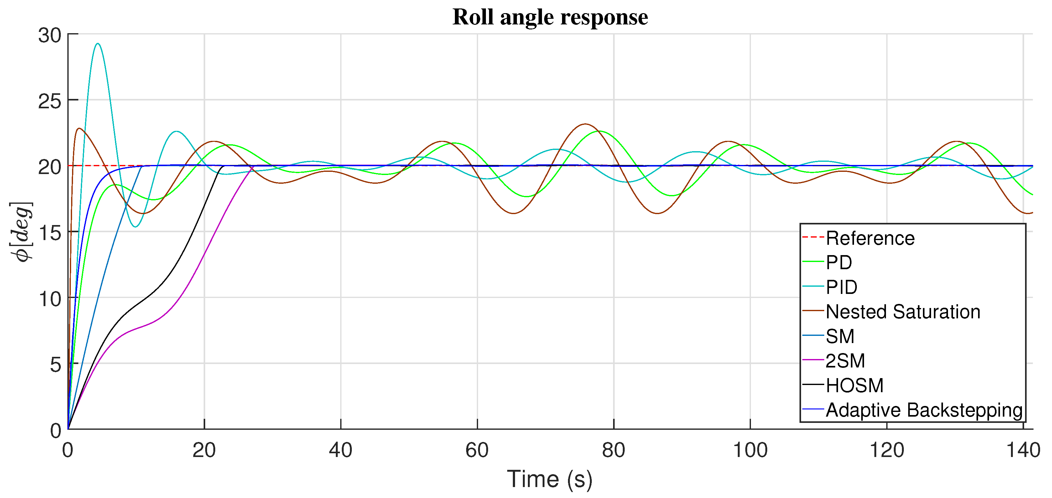
Figure 3.
PD control response in roll angle (with disturbances).
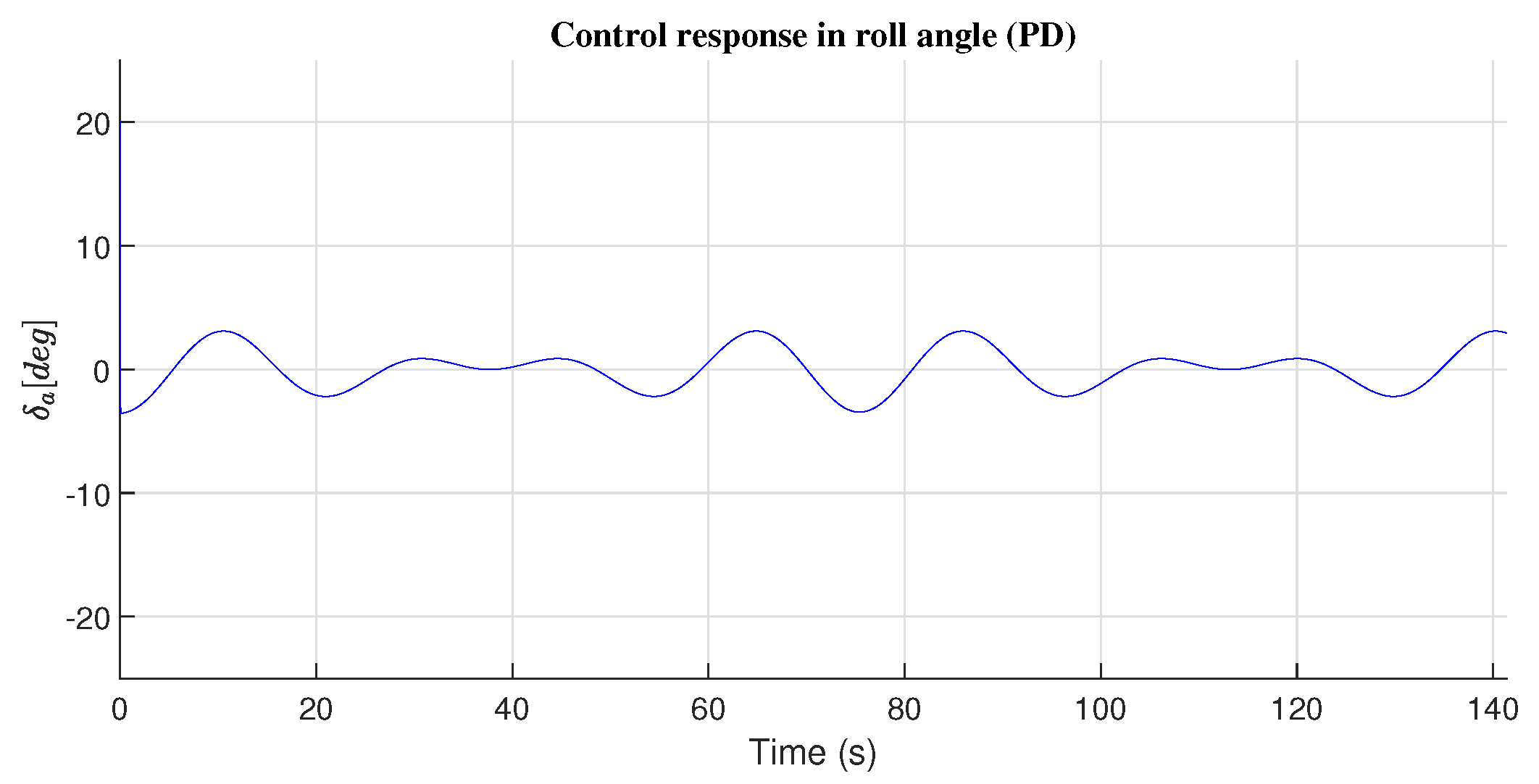
Figure 4.
PID control response in roll angle (with disturbances).
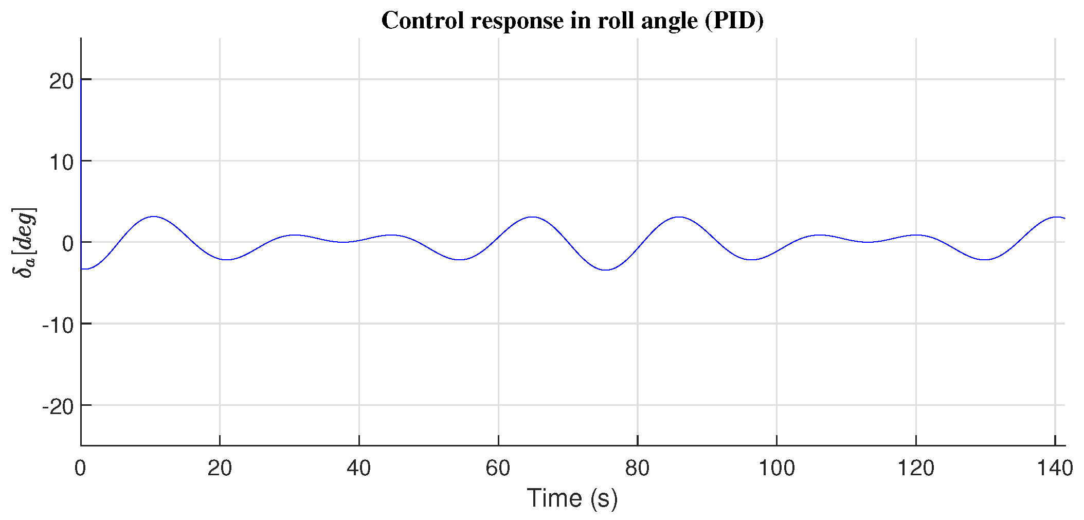
Figure 5.
Nested saturation control response in roll angle (with disturbances).
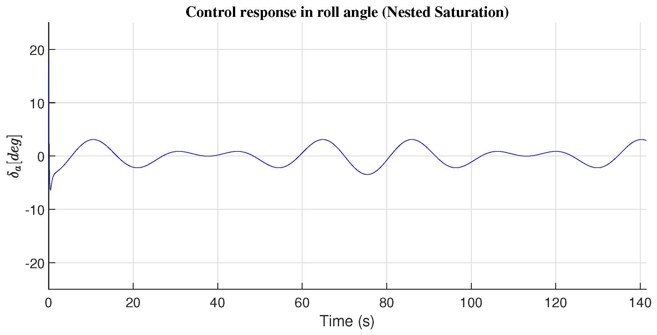
Figure 6.
First-order sliding mode control response in roll angle (with disturbances).
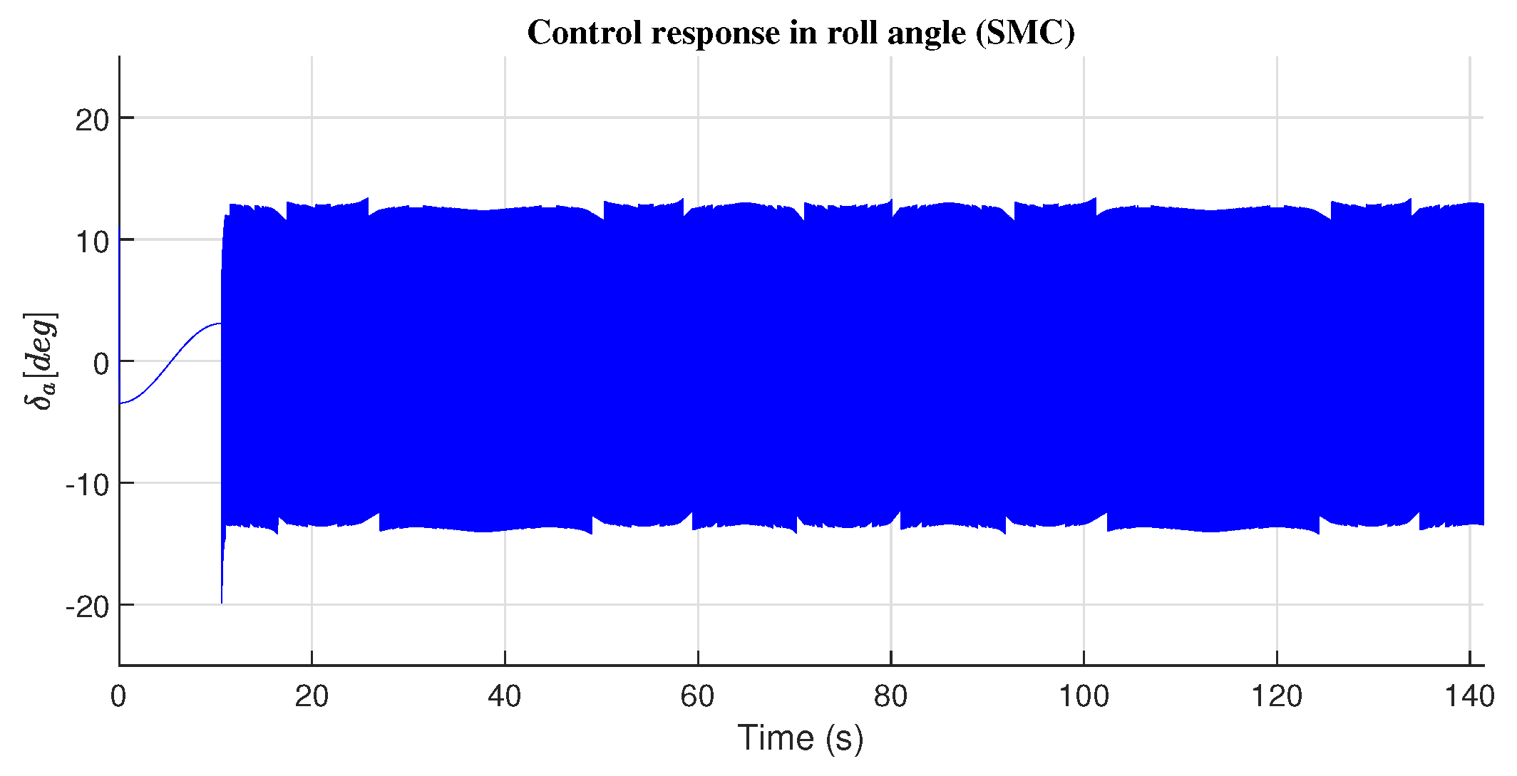
Figure 7.
Second-order sliding mode control response in roll angle (with disturbances).
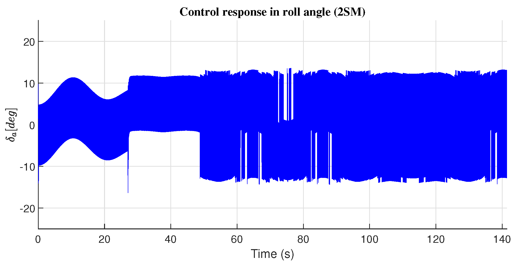
Figure 8.
High-order sliding mode control response in roll angle (with disturbances).
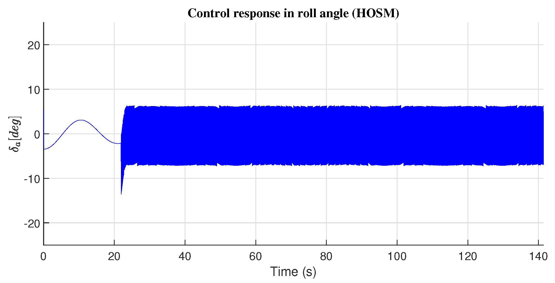
Figure 9.
Adaptive backstepping control response in roll angle (with disturbances).
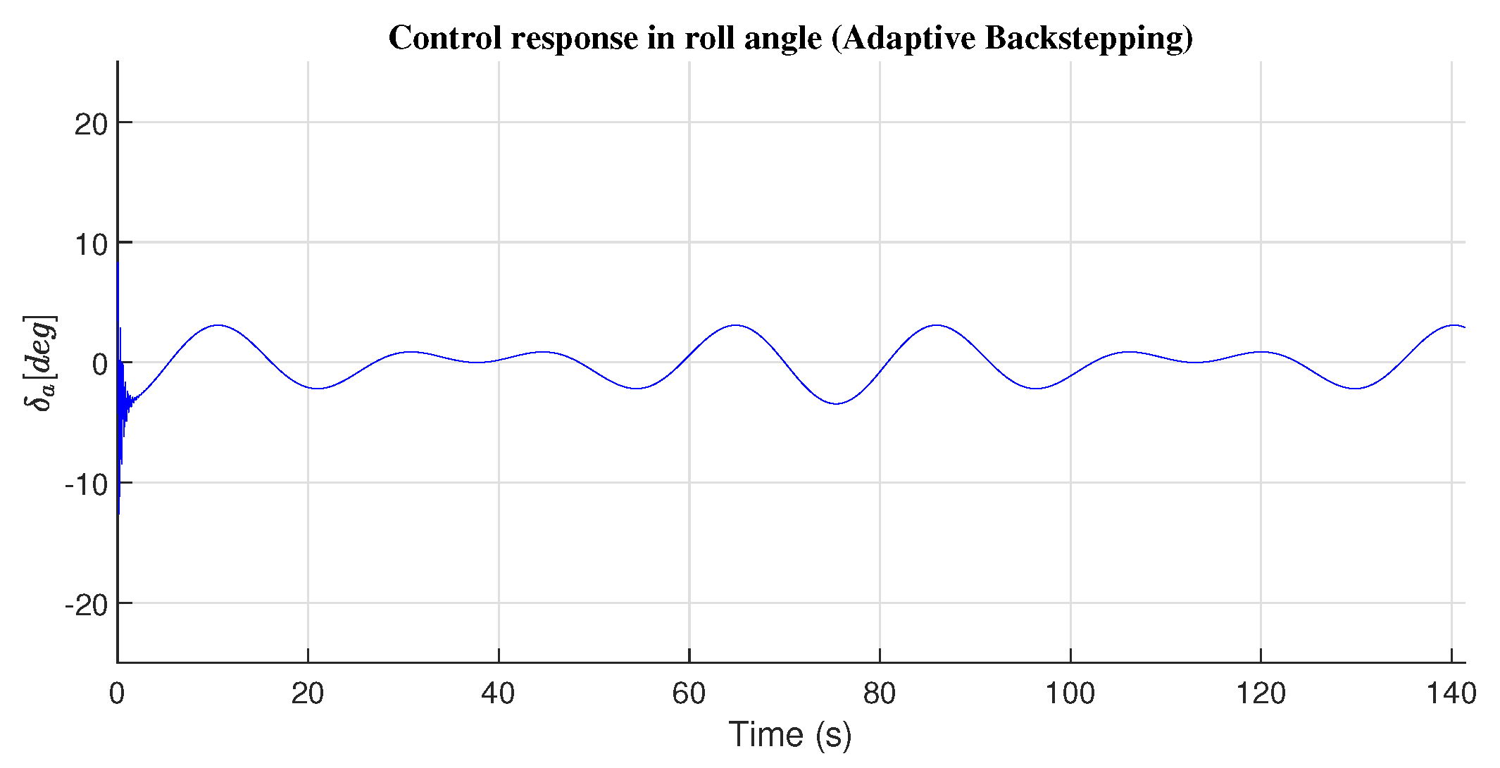
Figure 10.
Response in pitch angle (with disturbances).
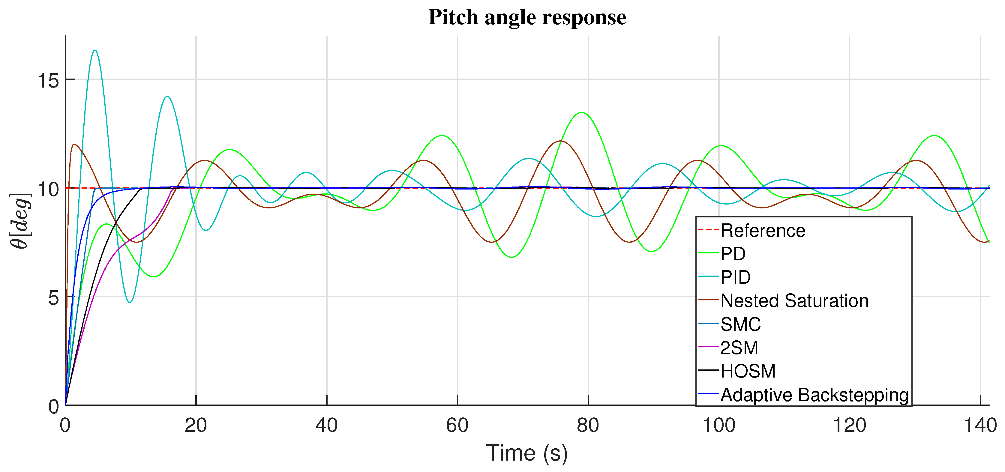
Figure 11.
PD control response in pitch angle (with disturbances).
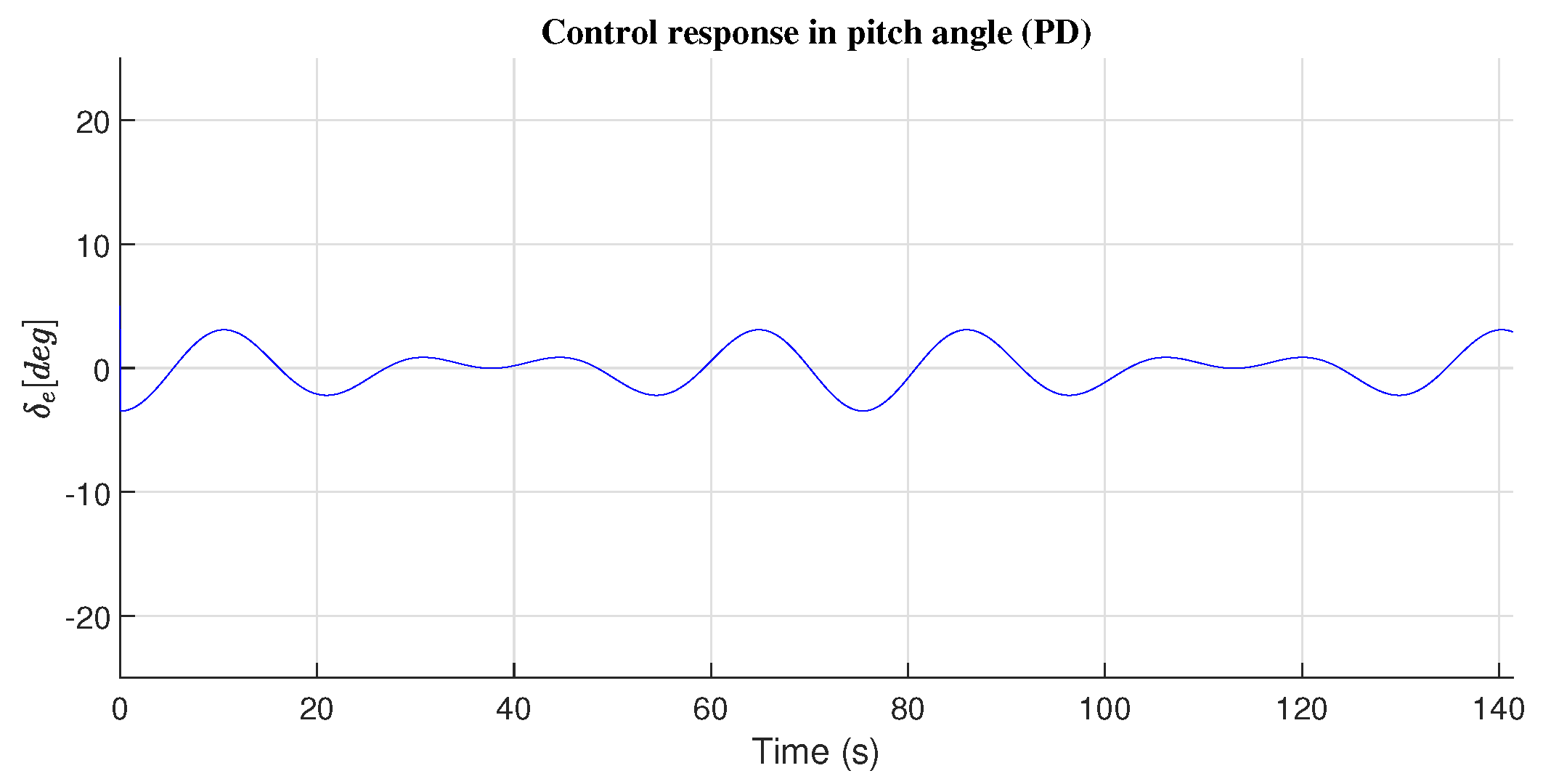
Figure 12.
PID control response in pitch angle (with disturbances).
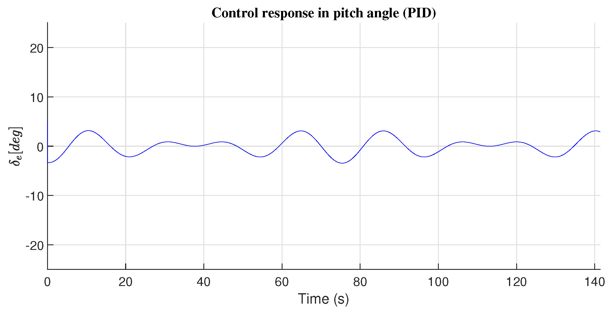
Figure 13.
Nested saturation control response in pitch angle (with disturbances).
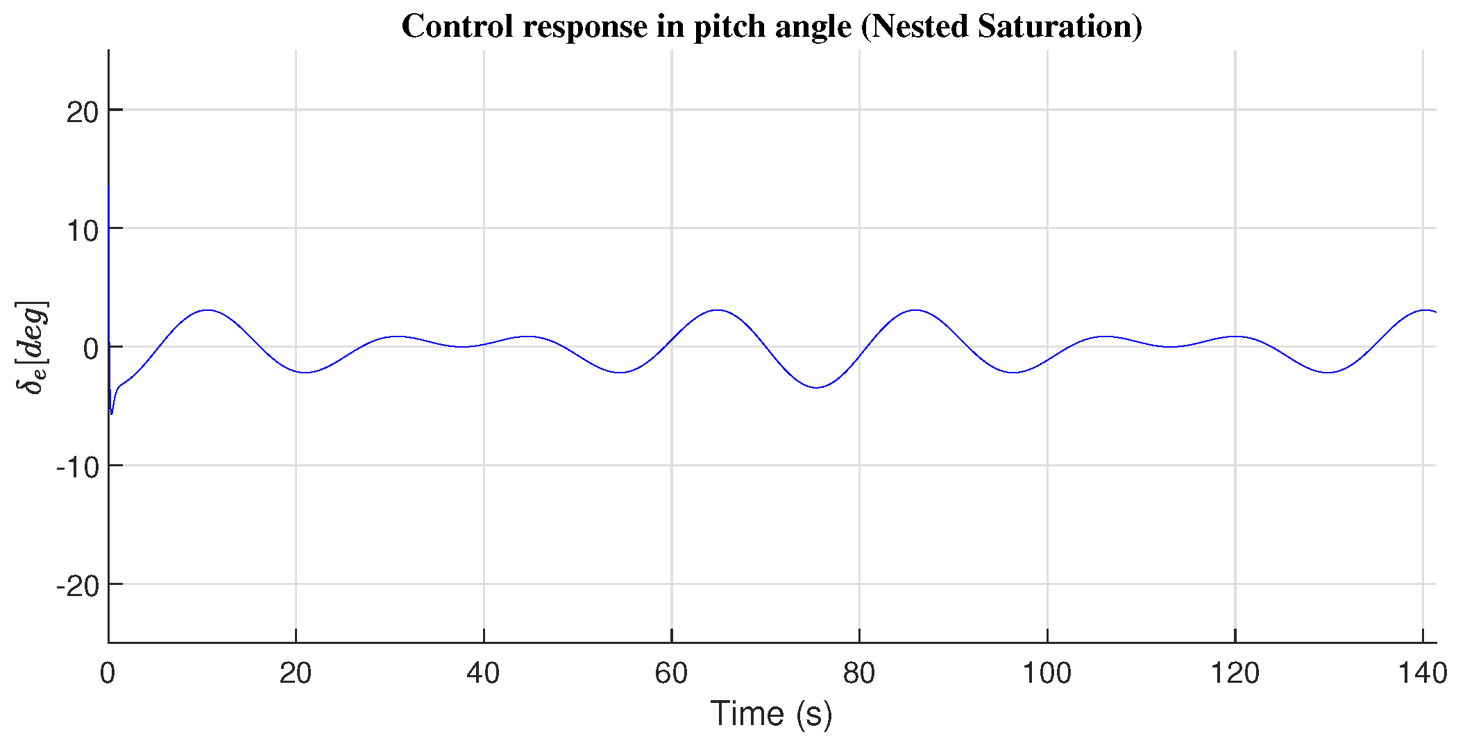
Figure 14.
First-order sliding mode control response in pitch angle (with disturbances).
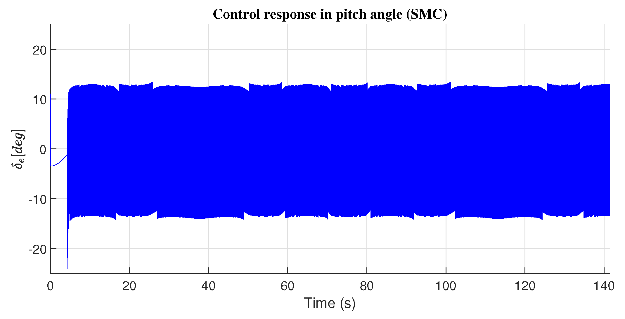
Figure 15.
Second-order sliding mode control response in pitch angle (with disturbances).
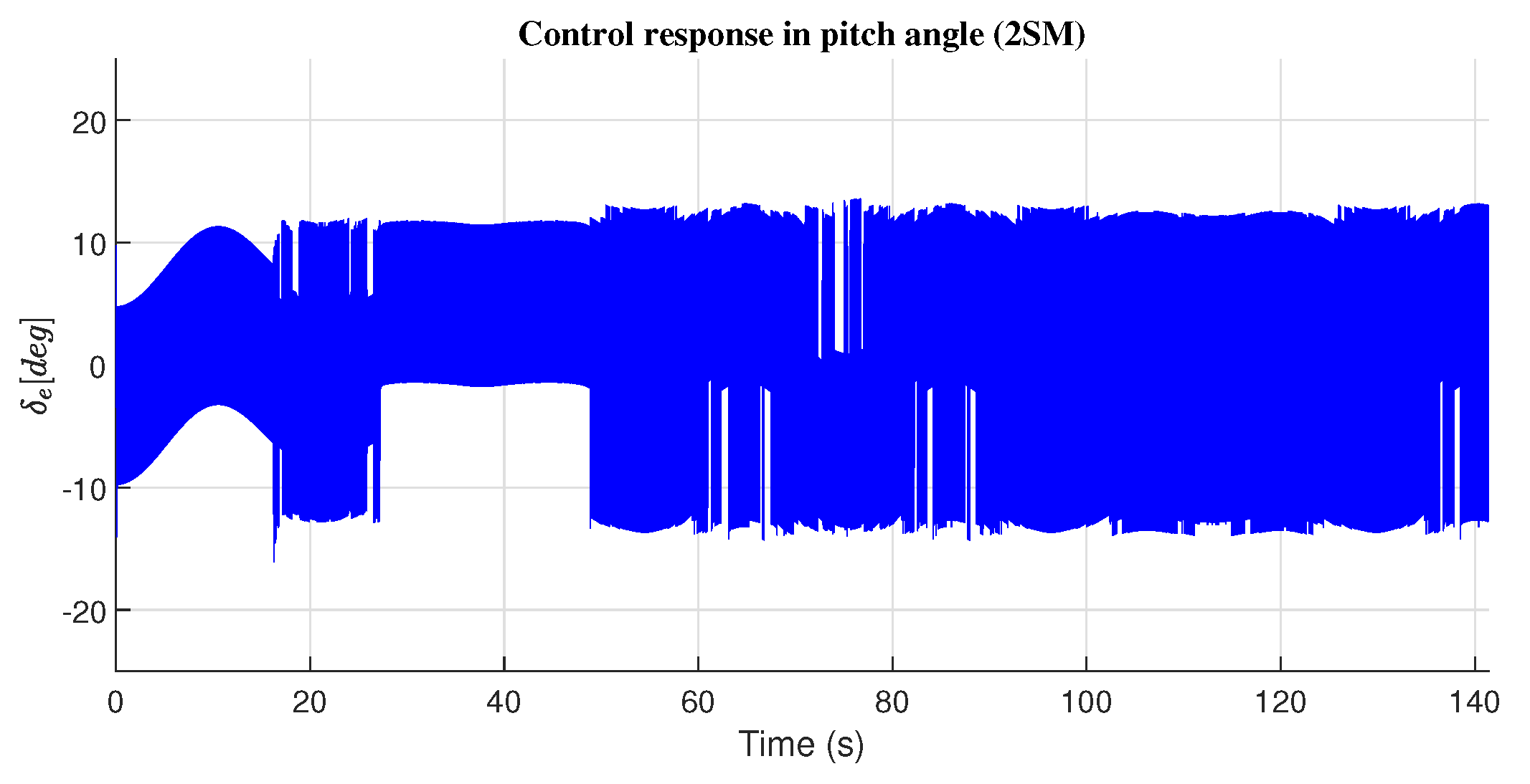
Figure 16.
High-order sliding mode control response in pitch angle (with disturbances).
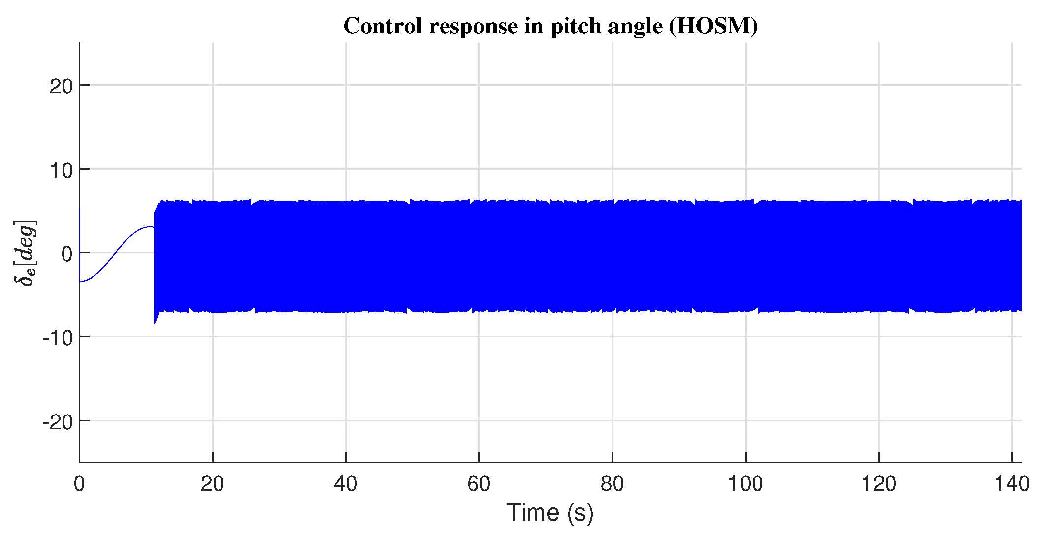
Figure 17.
Adaptive backstepping control response in pitch angle (with disturbances).
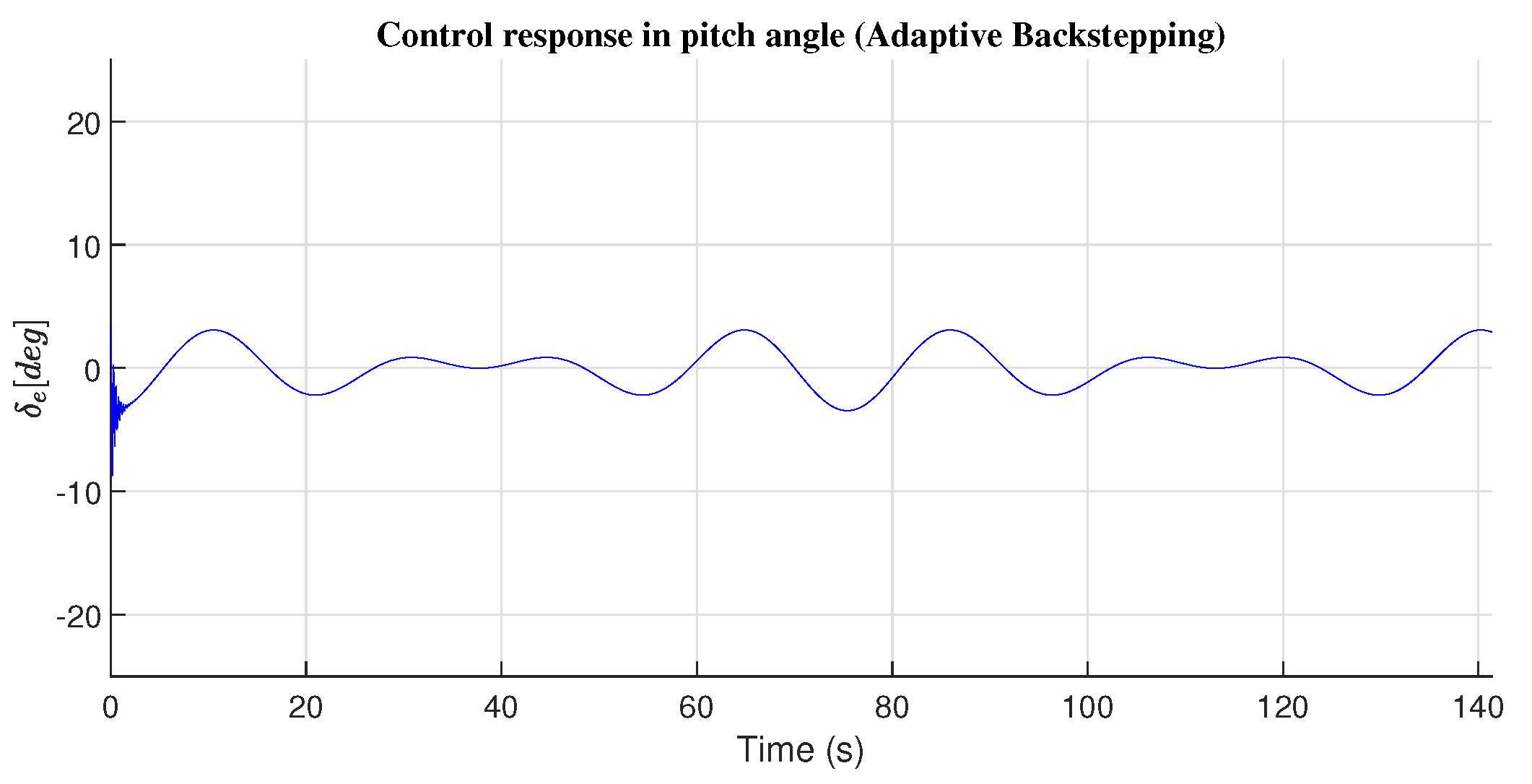
Figure 18.
Controllers response in X-axis (with disturbances).
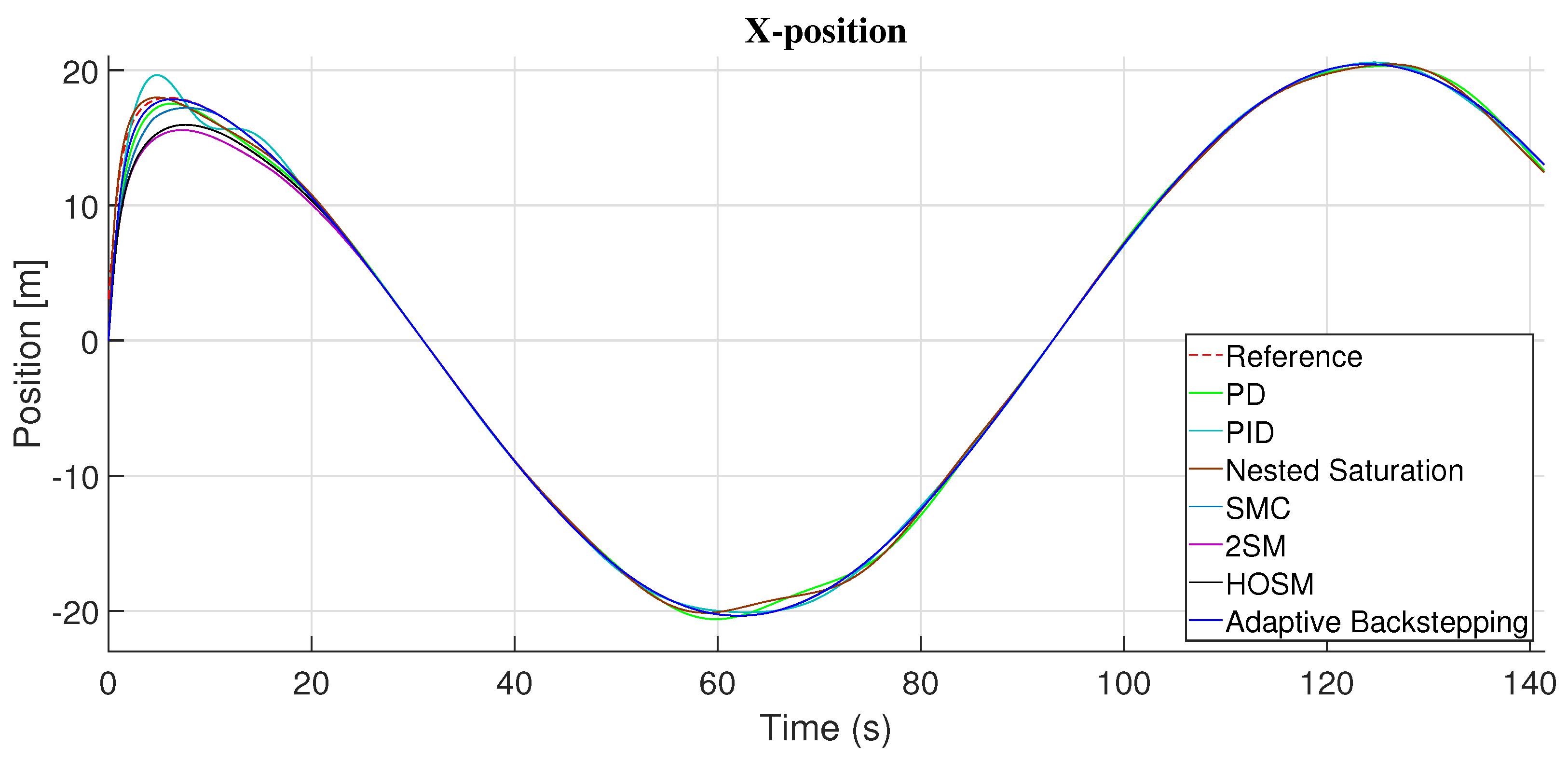
Figure 19.
Controllers response in Y-axis (with disturbances).
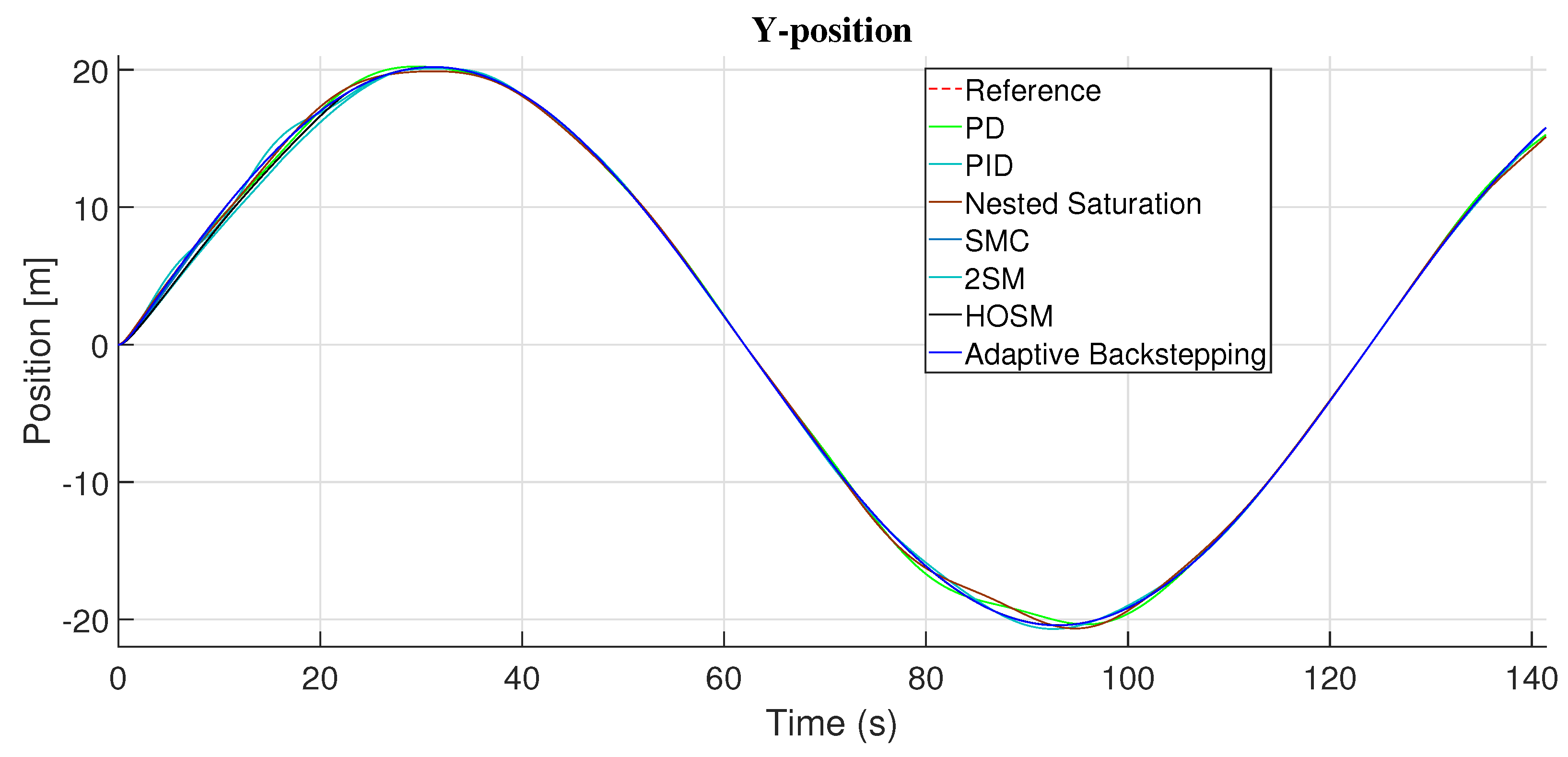
Figure 20.
Controllers response in Z-axis (with disturbances).
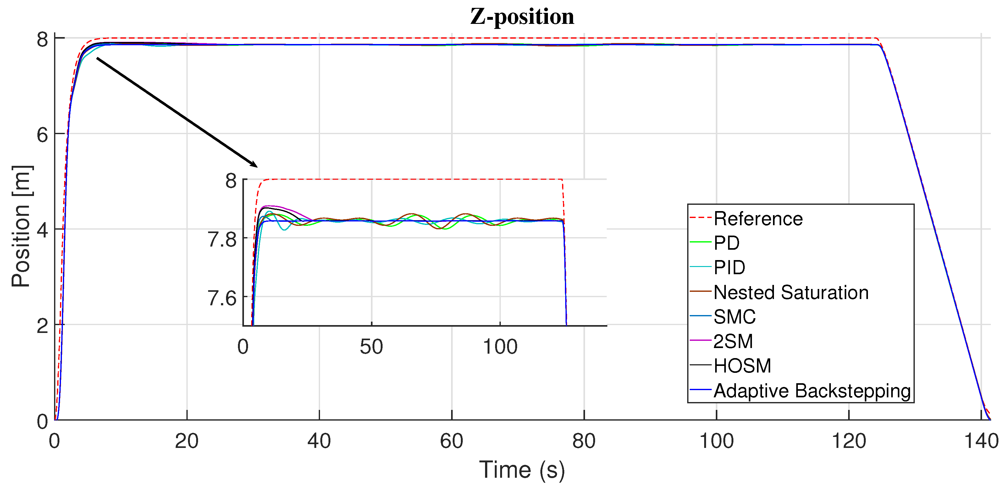
Figure 21.
Trajectory in 3D (with disturbances).
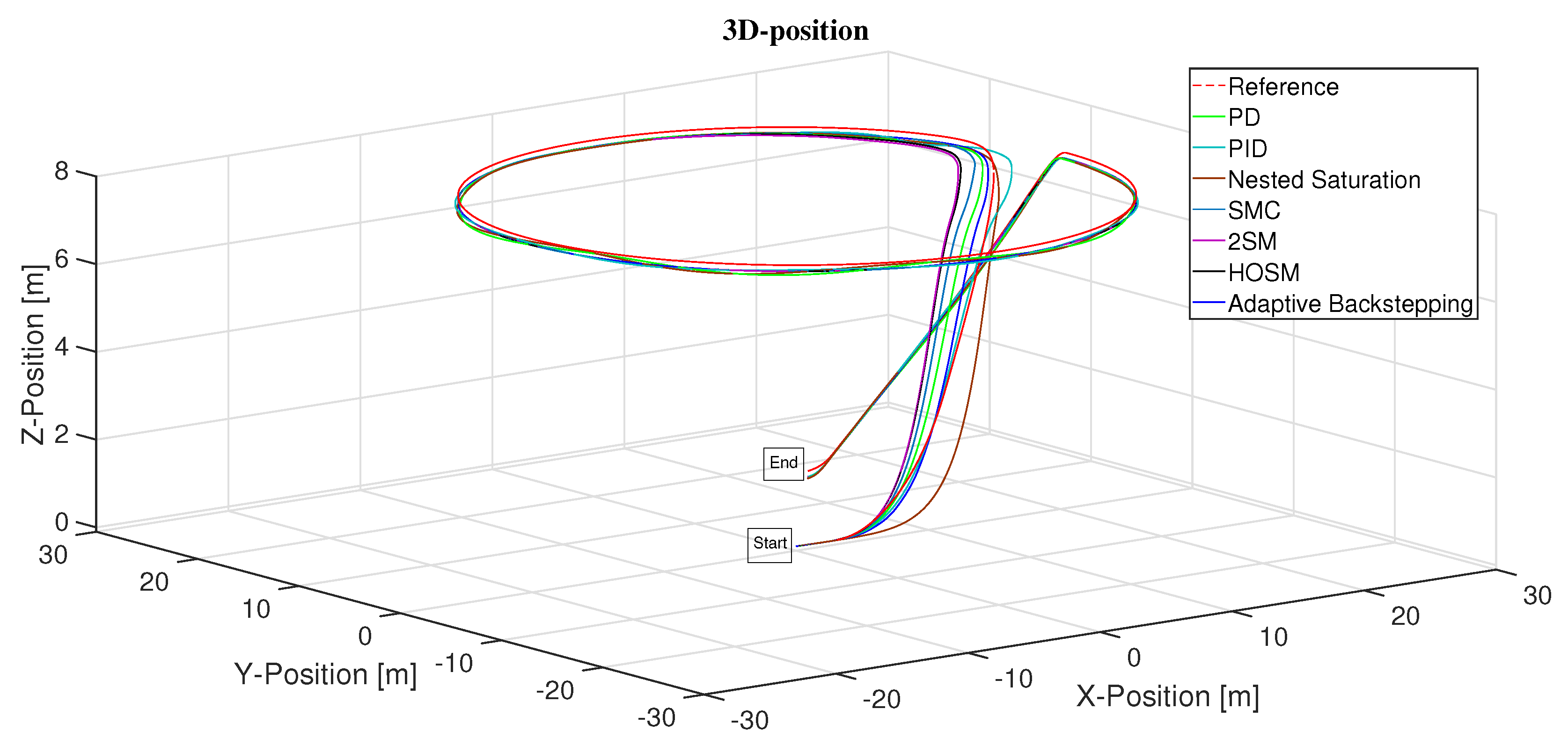

Table 1.
error and control effort in roll angle
| Roll Angle() | ||
|---|---|---|
| PD | 2.2186 | 1.6902 |
| PID | 2.1366 | 1.6902 |
| Nested Saturation | 1.9771 | 1.7372 |
| Sliding Mode | 2.9122 | 11.8892 |
| Second-order Sliding Mode | 4.9947 | 6.2838 |
| High-Order Sliding Mode | 4.4072 | 5.6993 |
| Adaptive Backstepping | 1.5271 | 1.7194 |
Table 2.
error and control effort in pitch angle
| Pitch Angle() | ||
|---|---|---|
| PD | 2.0078 | 1.6830 |
| PID | 2.6340 | 1.6826 |
| Nested Saturation | 1.2741 | 1.7097 |
| Sliding Mode | 0.9995 | 12.1660 |
| Second-order Sliding Mode | 1.5125 | 6.3147 |
| High-Order Sliding Mode | 1.3462 | 5.9203 |
| Adaptive Backstepping | 0.7598 | 1.6931 |
Disclaimer/Publisher’s Note: The statements, opinions and data contained in all publications are solely those of the individual author(s) and contributor(s) and not of MDPI and/or the editor(s). MDPI and/or the editor(s) disclaim responsibility for any injury to people or property resulting from any ideas, methods, instructions or products referred to in the content. |
© 2025 by the authors. Licensee MDPI, Basel, Switzerland. This article is an open access article distributed under the terms and conditions of the Creative Commons Attribution (CC BY) license (http://creativecommons.org/licenses/by/4.0/).
Copyright: This open access article is published under a Creative Commons CC BY 4.0 license, which permit the free download, distribution, and reuse, provided that the author and preprint are cited in any reuse.


