
Submitted:
05 July 2025
Posted:
07 July 2025
You are already at the latest version
Abstract
The article is devoted to the control of multichannel objects by the method of numerical optimization. In this area, there are several not entirely accurate, but ingrained ideas and approaches that it is time to sort out in detail. For clarity, typical examples are considered that anyone can check using inexpensive software, which, moreover, can be obtained free of charge in a demo version. Programming in this software is easy with the use of intuitive buttons and options. Thus, solving the problems of designing a regulator for multichannel systems becomes available to anyone who has a mathematical model of the object. The theses are based on the theory and confirmed by examples. The principles of controlling two-channel objects are proposed, i.e. objects of dimension 2×2, which by induction can be extended to objects of dimension 3×3 and, possibly, further. At the beginning, the solution to the problem of controlling a two-channel object of dimension 2x2 using a PID controller of the same size or its simplest modifications. Next, the problem of 3×3 objects is solved. There are two main factors for the result: the presence or absence of dominance of the absolute value of the diagonal elements of the transfer function matrix of the object over the re-maining elements, as well as the selected optimization objective function. In the case of dominance, the control problem is greatly simplified; in its absence, it can be ensured in some cases by changing the channel numbering. Recommendations are given for the formation of the objective function. For the first time, the use of a fractional power in the objective function is proposed, the effectiveness of this approach is substantiated and shown. For the first time, an additional modification of test signals during optimization is proposed, the effectiveness of this modification is shown. It is also shown how the quality of control of some channels can be improved at the expense of some deterioration in the quality of control of other channels.
Keywords:
controller
; automation
; PID
; MIMO
; symmetry
; modeling
; optimization
1. Introduction
Control of objects with two inputs and two outputs, where each input affects each output, requires careful design of the controller [1,2,3,4,5,6,7,8,9,10]. In particular, examples of such objects are the problem of simultaneous stabilization of the power and frequency of a semiconductor laser by controlling its current and temperature, with the temperature controlled by a Peltier- based microcooler. Another example of such problems is the automatic mixing of several substances, when it is necessary to simultaneously control both the increment of the mixture volume and the concentration of each substance. Another example of such a problem is the well-known problem of filling a swimming pool, with the need for separate control of the flow rate and temperature of the water. Similar problems arise in controlling the movement of any vehicle, especially space, air and water. There are many examples of such problems in robotics, chemistry, metallurgy, and scientific research.
Let us consider the problem of controlling linear objects. The proposed approach can also be applied to nonlinear objects, but the obtained result should be more carefully checked for the case of test signals of different amplitudes. In general, the problem of controlling nonlinear objects is much more complex; it is not possible to consider it thoroughly enough within the framework of this article, except for such types of nonlinearity as limitation or relatively small deviation of the characteristic from the linear one (no more than 10%). The discussed method is unsuitable for controlling objects with nonlinearity of the “dead zone” type, as well as “dry friction”, “hysteresis”, or other ambiguous nonlinearities. The proposed method is insufficient for controlling non-stationary objects; adaptive control systems are required for such objects.
The mathematical model of a linear two-channel object is defined in the form of a matrix transfer function [11,12].
There are many articles that talk about an object of size n×n, but no articles have been found with reliable information about successful control in such a formulation of the problem, i.e. with multichannel negative feedback and a multichannel sequential controller, even for objects of size only 3x3. Therefore, the term “multichannel objects” should be recommended to be used more carefully than is currently accepted in the literature. “Two-channel” would be more correct if even “three-channel” ones are not involved. However, we have verified our theses for validity by induction on the example of an object of size 3x3 and, if necessary, are ready to go further, to objects of size 4 x 4, but we do not know of such problems from practice, so we are in no hurry with these studies.
This approach should not be confused with multiparameter optimization problems or multicriteria optimization problems.
Control in a negative feedback loop is carried out according to the structure shown in Figure 1.
This structure best satisfies the requirement that the output signal should match its assigned value, called “Task”. Here, the element marked with a circle with a sign inside is an adder, but if there is a minus sign before the input, this input is subtractive. This and the following illustrations are made in the VisSim 5.0e software, which has some features for displaying various mathematical symbols, numerical values, and other elements. In particular, the minus sign looks like a hyphen, blue rectangles indicate composite blocks that have a complex structure inside, and their name is set by the user. Arrows indicate the direction of signals. When using the structure according to Figure 1, the task of controlling an object is reduced to calculating a mathematical model of the regulator (controller) based on a known mathematical model of the object.
2. Statement of the Problem
In the early stages of the development of automatic control theory, the control problem was posed and solved in terms of finding a control signal that must be fed to the input of the object so that its output values (called output signals) coincide with the prescription “Task”. This approach is impractical. The task can change, therefore, calculating the control signal loses its relevance. In addition, the object is always affected by factors that cannot be measured and taken into account in such a problem statement. The use of the structure according to Figure 1 is a different problem statement: instead of calculating the signal controlling the object, a mathematical model of the device is calculated, which itself calculates the necessary control signal depending on the task and the actual output signal of the object. A characteristic property of systems with negative feedback is that with a correct calculation of the regulator, the control problem is solved successfully even in the presence of unknown and uncontrolled effects on the object, which change its output signal in an unpredictable way. In the frequency band where the transfer function of the controller and the object connected in series with it is much greater than one, the output signal coincides with the task quite accurately. In this case, the difference between the output signal and the task, called the error, is inversely proportional to the product of the controller transfer function and the object transfer function. The problem with using this method is that any object has a transfer function limited by the frequency band. With increasing frequency, the transfer function decreases, although in some local frequency ranges it can increase. However, starting from some frequencies, it decreases so sharply that no amplification of the input control signal can achieve a significant response at the object output. For this reason, the transfer function of the entire loop in a conditionally open form inevitably reaches a value close to unity, and then decreases even more. In the frequency range where this value is much less than unit, the control loop no longer has a noticeable effect on the object, so its output signal in this frequency range is not controllable. We have to put up with this. But in the intermediate frequency band between those where the transfer function of the circuit is much greater than unit, which allows the object to be controlled, and those where the transfer function is much less than unit, which excludes the possibility of controlling the object, there is a frequency region where the transfer function of the circuit lies in the range from 0.1 to 10, i.e. from to . In this frequency range, the behavior of the transfer function of the loop affects the stability of the system. If at these frequencies the signal delay exceeds (or which is the same value in other measure units) then the system will be unstable. Therefore, the art of the designer of the locked dynamic systems consists in calculating such a controller that would ensure the stability of the locked system, as well as its sufficient accuracy in the frequency region where control is provided.
For multichannel systems, this is not enough. An additional property called “autonomization” or diagonal decoupling is required. It consists in the fact that any change in the task signal at any input should not only provide a corresponding change in the output signal at the corresponding output, but also that it should not affect the output signals of all other inputs. This requirement can be met only approximately. There was a scientific direction called “invariant control” that studied such control methods so that the control error was always strictly zero, but this area of automatic control theory has lost its relevance. The object is always affected by uncontrolled disturbing factors, which are usually described as an unknown interference, which is applied to the output of the object in the form of an additive unknown signal. Instead of the unrealistic task of completely eliminating the influence of disturbance, the modern section of control theory dealing with high-precision systems considers the problem of limiting the error to a certain value measured as a percentage of the task increment. An error of less than 5% of the task was considered acceptable at the early stage of automatic control theory; in modern high-precision systems, requirements are imposed to suppress the error to values of no more than 0.0001% and, in some cases, to an even smaller value. In problems of controlling multichannel objects, as a rule, the error is reduced to values of the order of 1–5% . In this case, we are talking about a dynamic error, since a static error, i.e. an error that is established after a sufficiently long time, provided that the task signals are step functions, can be reduced strictly to zero. This error does not include errors in measuring the output signal, which can never be reduced strictly to zero.
Thus, the problem of controlling an object, taking into account the above, is reduced to the problem of designing a regulator for an object with a known mathematical model using the structure according to Figure 1. Other structures and other formulations of the control problem are also known, which we do not consider in this article.
The controller for a linear object (1) can be represented as a matrix transfer function [13,14,15,16]. For example, for an object with two inputs and two outputs, such a transfer function has the following form:
In the simplest case, this matrix is diagonal, that is, only the diagonal elements are nonzero, and the remaining elements are equal to zero:
This means that there are only feedback connections from each output to the corresponding input and no other connections.
In more complex structures, additional loops may appear, for example, a loop that covers an object in addition to the device that subtracts the output signal from the task. There may also be a loop that covers the controller with feedback. The feedback may contain a transfer function that differs from unity. Ultimately, such modifications can be reduced by equivalent transformations to the structure shown in Figure 1, with the difference that the controller’s transfer function will be different, more complex.
The choice of a controller containing parallel proportional, integrating and derivative channels, which for this reason is called a PID controller, is determined by the fact that for the overwhelming majority of practical problems this choice is sufficient, and also by the fact that simpler structures in which one or two of the specified paths are missing are a special case of such a controller. These simpler structures can be obtained in special result in the same way as the design of a PID controller, which does not change the approach to the problem of controlling an object of type (1).
The development of computer technology and software has simplified the task of designing regulators for complex systems as much as possible [17,18]. For this reason, there is no need to even think about whether the problem can be solved using only a diagonal matrix regulator, or whether a full-fledged multichannel regulator with all non-zero elements of the matrix transfer function is necessary [19,20,21,22,23,24,25,26,27,28]. In many cases, it is sufficient to simply calculate a full PID controller, which in practice for objects of dimension and turns out to be insignificantly more difficult than calculating simplified diagonal controllers, as will be shown below.
The most common examples in the literature are objects with dimensions .
In this case, the object model is a matrix transfer function of the same dimension.
For control, a matrix PID controller of the same size is required [13,14,15,16,17,18,19,20,21,22,23,24,25,26], or perhaps a more complex version, for example, a controller containing additional channels of double derivation, double integration, both of these channels, or something more complex structure decision. For a PID controller, its individual elements are described by the sum of the proportional, integrating, and derivative channels with the corresponding coefficients:
The structure of the control system is shown in Figure 1.
3. Theory of Solving Problems of Multichannel Objects Control
The theory of locked dynamic systems is well developed: negative feedback ensures accuracy provided that the entire system is stable. Structural design consists of choosing the structure of the controller; parametric design consists of determining the parameters of the controller based on the chosen structure.
Structural design is not the subject of this article, since PID controllers are the most common, and the reason for this is their simplicity and efficiency. Simpler controllers, such as PI, PD, are not considered, since such simplification does not greatly simplify the method, but limits its capabilities. Complication by introducing additional channels of double integration or (and) double derivation is also not considered, since the approach under consideration can easily be extended to these structures. Structures with a large number of additional loops, such as the Smith predictor, local and pseudo-local connections, etc., are not considered due to their excessive complexity and low efficiency, which has also already been confirmed by modeling and practice.
Parametric design in our case is the main content of the system design task. Methods for calculating the parameters of the regulator can be grouped into large sections: analytical, engineering, tabular, empirical and numerical.
Analytical methods are based on the direct solution of matrix equations, which leads to the Riccati equation. If the matrix transfer function is not degenerate, it can be inverted. Inversion of this matrix is one of the important elements of solving the problem under consideration analytically. Even if the control problem is formulated in a different mathematical formulation, analytical methods cannot do without inverting the matrix transfer function of the object.
An inverse matrix is a matrix that, when multiplied from the right or left by the original matrix, yields the identity matrix. If the matrix transfer function has at least one delay link, the inversion of such a matrix transfer function yields a transfer function that cannot be implemented as any real device.
Let’s look at an example.
Inverting this matrix gives the following result:
Indeed, it is easy to verify that multiplication from the left or right by this matrix yields a unit matrix. But the resulting matrix consists of functions that cannot be implemented in any physical device. The fact is that the function describes in operator form (in the form of Laplace transforms) such a transformation of the input signal, which consists in delaying the input signal by time . However, at the same time, the transfer function describes such a transformation, which forms an input signal at the output of the element with a negative delay, that is, seconds earlier than this signal arrived at the input of the element. Such a “signal prediction link” cannot physically exist, it is something like a hypothetical “time machine”. Thus, if there is a delay in the model of the object, then analytical methods cannot be applied to the calculation of the regulator for such an object, or it is necessary to invent methods for reducing the delay to some other mathematical description, for example, to the Padé approximation. But such an approximation makes all calculations excessively complex and yet unreliable, and the result of the calculation is unreliable. The main objection to this approach is based on the fact that any mathematical model of any real object that does not take into account the delays of this object is insufficiently detailed for its effective use. This thesis is substantiated in Appendix A.
Tabular methods such as the Cohen–Kuhn, Ziegler–Nichols, Cohen–Coon, as well as Chien–Hrones–Reswick method and similar ones [29] are always unreliable, so they are hopelessly outdated. These methods are based on the assumption that the mathematical model of the object is described accurately enough by a series connection of a first- or second-order filter and a delay element:
Tabular methods suggest obtaining a graph of the transient process as a reaction to a single step jump, then using this graph to determine several basic parameters of this model. Then, using the table, one should determine the parameters of the PID or PI controller for such an object. A modification of this method is another method, in which the object is covered by proportional negative feedback, after which the coefficient of this feedback is selected so that undamped oscillations of constant amplitude are established in the system. Then, using the frequency and amplitude of these oscillations, the coefficients of the PID controller are also calculated from the table. All such methods rarely give an acceptable result, and they never give the best possible result. The problem with them is that they often result in an unstable system.
Some authors report that after using one of the tabular methods they slightly adjusted the coefficients, as a result of which they obtained satisfactory results. But in this case it should be recognized that the tabular method could not have been used at all; it would have been enough to set arbitrary coefficients of the controller, and then adjust them. This empirical method of adjusting controllers is widely used. It is used much more often than it is stated in articles, because the fact of using the empirical method does not provide grounds for writing a scientific article. The coefficients of the controller are simply successively increased until the stability in the system is violated, after which they are reduced to a value at which stability is restored.
Engineering methods consist of constructing an asymptotic logarithmic amplitude-frequency characteristic, as well as a phase characteristic with subsequent use of the logarithmic Nyquist-Mikhailov stability criterion. These methods work well for single-channel systems, but they have not been developed for multichannel systems, and it is too late to develop them, since they are morally obsolete. Before the active use of computing technology, constructing logarithmic graphs was much more effective and simpler than constructing graphs on a linear scale. An effective technique for constructing such graphs and their use for analyzing the stability of a system was developed, as well as for ensuring stability by correcting the logarithmic amplitude-frequency characteristic. A method for calculating a mathematical model of a correcting device based on the obtained logarithmic amplitude-frequency characteristic of this device is also known. At present, constructing logarithmic graphs that approximately describe the control object is already a more complex technique than numerical optimization. Thus, for linear objects with delay, the best method is a numerical optimization method, and if the object has at least the simplest nonlinear component, then the numerical optimization method is the only reliable method that allows obtaining adequate results with the least labor costs.
The most reasonable approach is a preliminary attempt to design a PID controller [30,31,32,33,34,35,36,37,38,39,40,41,42,43,44,45,46,47,48,49,50,51,52,53,54,55,56,57,58], since its simplification is not advisable, since this only slightly simplifies the design procedure, and its complication may be inappropriate due to the excessive complexity of this procedure and due to the insufficient efficiency of this measure in many practical cases.
The assertion about the insufficient efficiency of more complex structures is based on the fact that many types of complication of regulators lead to non-rough systems. Non-rough systems are those systems in which an insignificant deviation of the values at least one of all coefficients of the mathematical model of the object or regulator causes significant and even fatal changes in the type of transient process, including a violation of the stability of the entire system. Such methods leading to these undesirable results include the Smith predictor method, the method with high-order derivation, the method with a compensator, i.e. an element that is connected in series with the regulator so that in this element the numerator of the transfer function contains completely or partially the problematic factors of the denominator of the transfer function of the controlled object.
The advantage of numerical optimization is the ability to obtain results automatically. Only simple computer is necessary as well as free or inexpensive software and mathematical model of the object, as well as knowledge that can be acquired in the relevant literature, taking into account the recommendations of this article. The disadvantage of the numerical optimization method is the impossibility of solving the problem in general. Any solution is relevant only for a mathematical model with specific numerical values of all parameters of this model. However, some deviations of the actual values of the model parameters from the values used for the calculation are still allowed. If the solution remains relevant with a deviation of these parameters by 1-2%, the solution can be called rough. If the solution remained relevant even with a deviation of the parameters by 5-10%, this solution would be clearly robust. However, this is not always possible. If the model parameters can deviate from the calculated values, then an adaptive control system is required, which is not considered in this article.
Before describing the solution to the problem, we will establish the requirements for the transfer function of the object (1), necessary for the problem to have a solution. First, the matrix transfer function of the object (1) should not be singular. Its rank should coincide with its dimension; in this case, the rank should be equal to 2. In addition, it is highly desirable, although not necessary, that with the matrix should also be non-singular. If this matrix is singular, then control in the static mode will have some features [58]. They consist in the fact that even in the static mode, the control signals cannot be static. That is, to ensure that the output signals of the object take the prescribed value in the steady-state mode, it is not enough for the control signals arriving at the input of the object to have some necessary static value; these signals will have to change over time even to ensure a steady-state output state. This can be proven theoretically and experimentally [58].
4. Method for Solving the Problem
In general terms, the solution method consists of using the following initial means: a) software for modeling and optimization; b) test signal; c) modeling conditions (time sampling step and modeling time); d) objective function; e) optimization method; f) result analysis method; and g) method for improving the result if it is not good enough.
The question naturally arises: “If the result is optimal, then how can we raise the question of its further improvement?”
However, the point is that the objective function is not the only option that follows from the control goals. For a set of control goals, the most diverse objective functions can be substantiated, formed and used. In addition, the result also depends on the modeling conditions and on the weight coefficients in these objective functions, on which the method for further improving the result is based.
The optimization method deserves special comments. If the optimization is successfully completed, then it makes no difference which optimization method was used. Any optimization method that gives a result should give the same result within the permissible error. If different optimization methods give different results, this indicates an error in solving the problem. Most likely, this can happen when the objective function has several local extrema. In this case, a designer can distinguish a local extremum from a global one by the value of the objective function at these points. If the minimum of the function is sought, then at the point of the global minimum the objective function takes the smallest value, and at the points of the local minimum, its value is greater.
If one of the numerical optimization methods does not lead to the desired result, and another method does, then the system designer can simply use the results obtained by a more effective method, and there is no need to think about the reasons why the other method was unsuccessful. Therefore, if somebody were able to buy the required product in one store, he is no interested in the reasons for the absence of this product in other stores. In general, various optimization methods can be theoretically analyzed and the different efficiency of various methods can also be theoretically substantiated. Although experimental substantiation is quite sufficient to move on.
Finally, if none of the numerical optimization methods embedded in the software leads to the desired result, it is necessary to find out the reasons for this. Instability of the optimization procedure is most often a consequence of an insufficiently effective objective function. The objective functions and their modifications proposed in this article do not cause problems except for those cases when the problem cannot be solved by numerical optimization methods due to the absence of a global minimum for the mathematical model of the used object. This issue is also discussed below in Appendix A.
In the VisSim 5.0e, as in other versions of this software, there are two types of optimization. One of these types is the search for parameters that give the objective function a zero value. We do not use this type of optimization for the problem under discussion. The other type of the optimization that we use is the search for parameters that give the minimum of the positive-definite objective function, which in this case is called the “cost function” or simply “cost”. We will use this name further.
The method we propose is developed and described in some detail in our publications [11,12,17,18]. To solve the problems of control of multichannel objects, some modification of the cost function is required.
The cost function for this case is the sum of the cost sub-functions for each individual channel [58]. For each channel, such a cost sub-function is the sum of the integral of the error modulus multiplied by the time from the start of the transient process during the process , and penalty additives . One of the most effective penalty additives is the positive part of the product of the error and its derivative [11,12,17,18].
The first member of the cost function has the following form:
The second term is determined by the following relationship:
Here
Thus, the cost function has the following form:
The following modifications of the cost function components can also be used:
We will show in the examples below for what purpose it is possible to use a fractional power of the values included in the objective function, in particular, the square root of the signal or the fourth root. The rationale for using the square root is that the product of the error and its derivative is a quadratic form, which is proportional to the square of the error amplitude. This is not desirable, because we optimize linear system. The result should be invariant to the value of the test signal. So using the square root is a natural solution that has not been previously published yet. Modeling has shown that this improves the performance of the cost function.
The rationale for using the fourth root is based on two arguments. The first argument is that if introducing a square root improves the result, it is useful to try to apply a higher order root by induction as well. The second argument for this approach is that such a nonlinear function increases the contribution of small signals. This allows for a reduction in small signal deviations from the desired value when large deviations are already sufficiently suppressed.
During modeling, it is necessary to feed a test signal to the system model, which represents a task for the system, that is, a vector of input signals describing the desired values of the vector of output variables of the control object.
Since independent control of each output is required, the individual components of this vector must be substantially different functions and there must be no linear relationship between them. Traditionally, when optimizing a scalar linear system, a signal in the form of a single step jump is used [11,12,17,18]:
Here is the time discretization step. For this reason, the task vector is proposed form in the form of stepwise jumps, shifted relative to each other by half the time of the transient process simulation [58]
In this case, instead of a multiplier proportional to the time from the start of the transient process, a sawtooth signal should be used, linearly increasing from the moment to the moment , after which it resets to zero and again linearly increasing from zero at the same rate.
A delay in the occurrence of a step jump by at least the value equal to the doubled time sampling step is a mandatory condition that we have not encountered anywhere in the literature, but on which we have grounds to insist. If a jump at the input occurs without such a delay, then the simulation results may not coincide with the practical results, since in this case the system processes not the jump, but the initial state of the object, the results of signal differentiation in the system in this case will differ. A reliable check of the quality of the system is based on its operation when step jumps are supplied, and not on the type of processing of the error of the initial state. In the practice of modeling and optimization, we have had cases when the results of modeling in these two non-coinciding modes were noticeably different.
VisSim software (in any version) contain a mixture of functions in the time domain and functions presented as transfer functions, i.e. in the Laplace transform domain. There is no contradiction in this, since no error will arise. The mathematical notation of equations in such a mixed form would be erroneous, but the mnemonic designation of the blocks used in programming the project is quite understandable and for this reason acceptable. The VisSim software, designed for modeling and optimizing automatic control systems with feedback, uses various mathematical models. It contains models of linear elements that are described by transfer functions in the Laplace transform domain, as well as models of nonlinear connections that are described in the time function domain, and other elements. The software does not require uniformity of terminology, since it is not necessary to create full mathematical model of the system in the form of the one-type equations in the standard form for all of then form as correct mathematical description. The model is created from individual elements, between which, when this model is graphically specified, the appropriate connections are established from the inputs to the outputs; different ways of describing individual elements are not a problem.
5. Statement of the Problem
Example 1. Let us consider an object whose transfer function has the following form:
We consider such objects for the following reason. A set of simple hypothetical models most accurately reflects all aspects of the possible problems considered in this article. Since not the only favorable type of models was used, but the inverse variant was also investigated, then the view to the chosen part of the problem can be treated as the researched one. More complex objects in the class of ones considered in this article are characterized by positive poles of some polynomials in the denominators of most specific elements of the transfer function. We do not consider such problems in this article. It is in our plans for the future.
If the polynomial of the transfer function denominators has no positive roots, then any example of the same order (an object of dimension , polynomials in the denominator of dimension 2, polynomials of order zero in the numerator) will not be more difficult than the examples considered in the article. If the polynomial of the transfer functions has positive roots, then slightly different methods are necessary, including, for example, non-linear controller or some others.
6. Methods of Problem Solving
When modeling in the VisSim software, the object is formed from four models, which are shown in Figure 2. It should not be surprising that the coefficients of the free terms in the denominators of all transfer functions are equal to unit. This is the canonical form of these functions, since if this were not so, then the numerator and denominator of these transfer functions would be sufficient to divide by these coefficients to bring them to the canonical form. In this form, the transfer function at becomes equal to the coefficient in the numerator.
VisSim has three built-in numerical optimization algorithms. The Powell method, the Polak-Ribiere method, and the Fletcher-Reeves method. These methods are well known enough to be described in this paper, and, moreover, the possibility of using these methods is entirely due to the developers of this software; a description of these methods is beyond the scope of the authors of this paper. We have repeatedly found empirically that the Powell method is the best for this class of problems, since in many cases when one of the other two methods fails, or even both, the Powell method still succeeds, resulting in a set of optimal parameters, i.e., parameters that give a minimum value to the cost function. If any of the other methods works, then it gives exactly the same result as the Powell method. For this reason, there is no point in using the other two numerical optimization methods. And there is no point in describing the algorithm of the Powell method.
Powell’s method is based on the calculation of tangents and the assumption that any line passing through an extremum point intersects tangents to points of equal value of the objective function at the same angle. The other two methods are based on the calculation of the gradient of the objective function, which has a chance of unstable operation near the extremum point. At these points, the gradient is small and the influence of noise or random factors can lead to wandering around the extremum point. However, if the problems discussed in Appendix A do not arise, then all three built-in optimization methods can give the same optimization result.
7. Results
7.1. Two-Channel Object with a Majorizing Main Diagonal
Figure 3 shows the design for optimizing the controller for this case. In this figure, the individual PID controllers and the transfer function elements of the plant are combined into composite blocks called “PID” and “Compound”, respectively.
Figure 3, like the following figures, requires some preliminary comments. All these figures were obtained by screenshot from the VisSim software, so they have not been edited. Rectangles with an asterisk symbol inside denote signal multiplication devices. Rectangles with the inscription «pow» denote power raising units, unless otherwise specified in the text, this is the second power. Rectangles with the inscription «derivative» are input signal derivative calculators, rectangles with the symbols «1/ S» are integrators, a rectangle with a step or sawtooth signal drawn inside is a signal generator of this type, a rectangle with the inscription «abs» is an absolute value calculator of the input signal, a rectangle with the inscription «cost» is the input of the optimization device, where the calculated cost function is fed, which makes it possible to program the formula for its calculation.
The remaining rectangles are bus labels; they give the name to the buses or the quantities used. For each identical mark, it is considered that they are all connected to each other, and only one such block can be supplied with a signal; the program does not allow supplying another signal to another such mark, which is a natural limitation. In addition, the signal value of each mark can be used as a gain factor in another place. The blocks that set the gain factor have the form of a pentagon. In order to set the value of the variable gain factor in this way, it is enough to enter the name of the corresponding bus in the field for recording its value. Also, instead of the bus name, an ordinary number can be written in this field. Decimal numbers in this program are shown in a special format: if the number is less than zero, then the zero before the decimal point is not written, in negative numbers in this case there is a hyphen before the point, denoting a minus. The exponent is written after the number and separated by the letter “e”. Different colors of the lines correspond to the coloring of the input arrows. In particular, the output signal of the first channel is fed to the oscilloscope through the red arrow, so it is displayed as a red line. The output signal of the second channel is fed through the blue arrow and is displayed by a blue line. In all graphs here and below, the abscissa axis shows time in seconds, and the ordinate axis shows the output signal in conventional units.
The output values of any controlled object are physical values. These can be voltage, displacement, heating, rotation angle, etc. Each such value is measured by the corresponding sensor and then compared with the task. When modeling, it is not customary to write the physical units of these values, because control theory does not consider the absolute values of the output values, but only their increments in relation to the initial equilibrium state, and they are most often normalized, that is, divided by some standard value, so that only increments in relative units are displayed on the graphs. For linear systems, this is absolutely normal, since scaling the signal does not change the nature of the graphs. We do not consider nonlinear systems in this article.
The monitors on the center of Figure 3 show the obtained values of the corresponding coefficients of the matrix PID controller.
All the above mentioned approaches to optimization were applied here.
The software for modeling and optimization is VisSim 5.0e. This program is optimal for such tasks. Unlike MATLAB Simulink this software simply does not allow modeling of objects that cannot be implemented in practice. This software takes up little space on the disk, and the files it creates also take up little space. The main advantage is the precise reproduction of the algorithms by which real digital regulators operate.
The test signal, as indicated above, is single step jumps, shifted relative to each other by half the simulation time (15).
The simulation conditions are as follows: time discretization step and simulation time . The integration method is the simple Euler method.
The objective function (10) with its constituent functions (6), (7), (8), (9).
The optimization method is Powell’s method.
The method of analyzing the result is a visual assessment of transient processes, an assessment of the roughness of the solution by rounding the obtained coefficients to 1%, and, if necessary, also changing the parameters of the object model by values or more.
The method of improving the result is to change the weighting coefficients in the cost function. To eliminate overshoot, non-monotonicity, oscillations, it is necessary to increase the weighting function for the term that depends on the positive part of the product of the error and its derivative; to reduce the static error, it is necessary to decrease this coefficient or increase the modeling time. If this does not help to obtain the desired result, then also increase the modeling time, modify the cost function.
In this result we do not see overshoot in the transient process of each channel, but we do see the response of each channel to a task step in the other channel, and this response is about 10% of the corresponding step.
Modeling and optimization showed that further changes in the cost function, including changes in the weight coefficients of the terms dependent on the product of the error and its derivative, did not significantly improve the transient process. Any specific improvement in one of the parameters of the transient process is achieved only at the expense of worsening the other parameter. Namely: it is possible to completely suppress this reaction in the second channel by increasing such a reaction in the first channel and decreasing the response speed of both channels. Or it is possible to increase the response speed of the second channel and almost completely suppress this reaction, but at the expense of increasing such a reaction in the first channel to 18%. It is also possible to significantly improve transient processes in the first channel, but at the expense of significantly worsening the response of which channel: in it, the advising response to a jump in the task of the first channel increases to 18%.
It should be noted that a relatively successful solution to the problem is achieved due to the fact that the transfer function has advantageous combinations of elements. This property is hidden in the fact that, firstly, the diagonal elements contain transfer functions in which the transfer coefficients are significantly greater than similar coefficients in other elements of the matrix transfer function of the object. Secondly, these same elements have a smaller delay value. Thirdly, the denominators of these same elements has smaller coefficients at the terms of the second and third order.
For educational purposes it is advisable to use objects like Example 1. Also, if in a practical task this is what a designer should strive for and sometimes this can be achieved by correctly choosing the numbering of the inputs in accordance with the numbering of the outputs.
Let us show that the indicated relations simplify the solution of the problem. To do this, we will zero out the elements in the regulator matrix that are not on the main diagonal. To do this, it is sufficient to zero out the corresponding coefficients, as shown in Figure 3, and remove from the project the extra blocks «Parameter Unknown». As can be seen from Figure 3, which shows the resulting project, control remains successful and even the deterioration in control quality was not too great.
However, this is the case, since in this case the simulation time had to be doubled, and, accordingly, the transient processes doubled. If in Figure 3 the processes when applying a jump to the first input last 10 seconds, and when applying a jump to the second input last 20 seconds, then in Figure 4 the processes when applying a jump to the first input last 20 seconds, and when applying a jump to the second channel last 30 seconds.
7.2. Two-channel object with a majorizing small diagonal
Example 2. Let us consider an object whose transfer function has the following form:
This example is derived from the object of Example 1, in which the first column is replaced by the second, and the second column is replaced by the first. As a result, the transfer function of the object has become maximally unfavorable according to the criterion considered above. The elements on the main diagonal are characterized by a large delay, smaller transfer function coefficients, and large values of the coefficients in the denominator polynomials.
This example is one of the most unfavorable options for objects from this class.
Figure 5 shows the result of an attempt to optimize the diagonal regulator controller for the object of example 2. The attempt was unsuccessful, the system turned out to be unstable.
Figure 6 shows the project and the result of an attempt to calculate a full matrix PID controller for the same object from Example 2. A stable system is obtained. However, the quality of the obtained system is low. The overshoot in the first control channel reaches 98%. The overshoot in the second channel is 12%. The overshoot in the first channel with a jump in the second channel is 50%, the overshoot in the second channel with a jump in the first channel is 98%, as well as the reverse overshoot, which is about 50%.
In this case, the number of oscillations of all overshoots and with overshoot is at least 4 distinct oscillations. In addition, the duration of the process is very long, it is more than 60 seconds to the level of 5% and long residual relaxation processes of at least 40 seconds are also observed in the area of a small error. In addition, in the second channel, a second wave of response to a jump in the task of the first channel is observed, the peak of which is long and is between intervals of 20 seconds and 40 seconds.
From this example it should be concluded that with an undesirable combination of all parameters of the object model, multichannel control can be a rather complex task. However, this case is obviously bad; in practice, such cases should not arise, since the designer should pay attention to the fact that in the secondary diagonal all elements of the matrix transfer function have a significantly greater value in the entire frequency range for the reasons stated above. In this case, the designer should change the numbering of the outputs or the numbering of the inputs, which are the same in this case. To do this the output the first channel should feed the second input, and the output of the second channel output should feed the first input. This will result in the matrix transfer function of such an object taking the form given in Example 1, and this problem, as we have seen, is solved quite simply and successfully. This example shows that along with formal methods of designing controllers, a preliminary analysis of the properties of the matrix transfer function of the object should be used in order to identify the strongest channels of influence. In this case, the first input has the greatest influence on the second output, and the second input has the greatest influence on the first output, which dictates the choice of the rule for numbering outputs and inputs.
This approach is intuitive and should be used at an early stage of design, i.e., preliminary. For example, we want to move a tower crane load toward two directions and we have two adjustments, one for each arm. Let the left adjustment move the load strongly vertically, but weakly horizontally, and the right adjustment move strongly horizontally, but weakly affect vertical movement, then, when creating an automatic system, we should select the left adjustment to control vertical movement, and the right adjustment to control horizontal movement. Full autonomy will ensure that the left adjustment will affect only vertical movement, but will not affect horizontal movement, and the right adjustment, accordingly, will control only horizontal movement, but will not affect vertical movement. If the designer takes the opposite approach and tries to make the left adjustment control the horizontal movement and the right adjustment control the vertical movement, then the problem will still be solvable, but it will be similar to the one considered in Example 2, i.e. the least influential inputs are chosen to control these quantities, which complicates the controller design and can negatively affect the quality of control.
7.3. Two-channel object without an obvious majorizing diagonal
Example 3. Let us consider an object whose transfer function has the following form:
This transfer function is also obtained from the transfer function of Example 1 with appropriate permutations. In this case, in the first row, the most significant element is the element that is not on the main diagonal, and in the second row, the most significant element is on the main diagonal.
Figure 7 shows the structure project and the result of optimization of the full PID controller for such an object from example 3. This system is stable, but the response of the second channel to the step jump of the first channel is too large. It reaches 75%, and its duration is 30 seconds. The response of the first channel to the jump in the second channel’s task is 14%, its duration to the level of 50% of the maximum value is less than 5 seconds, but the duration of its noticeable part is about 40 seconds. In this case, control for each channel is carried out without overshoot; the duration of the processes is from 40 seconds (for the second channel) to 60 seconds (for the first channel).
It is also advisable to try to control this object using a simplified diagonal controller. Figure 8 shows the design and result of controlling the object of Example 3 using a diagonal controller.
In this case, the result is noticeably worse, but the resulting system is stable. The response of the second channel to the step jump of the first reaches 98%, and its duration is 50 seconds. The response of the first channel to the jump in the second channel task is 13%, its duration is about 40 seconds. In this case, control for each channel is carried out without overshoot; the duration of the processes is 50 seconds for each channel.
Example 4. Let us consider an object whose transfer function has the following form:
This transfer function is derived from the transfer function of Example 3, with the difference that the elements in the minor diagonal are negative. Figure 9 shows the design and optimization result of the diagonal controller for this case.
In terms of process quality indicators, there is no significant difference with the result presented in Figure 8: cross-responses and emissions are comparable in size and duration.
Figure 10 shows the design and optimization result of the full controller for the object from Example 4. When compared with the result shown in Figure 7, it has a slight advantage, namely: in Figure 6, the response at the output of the second channel with a jump in the reference at the input of the first channel is 75%, and in Figure 10, the corresponding response is 61%. In terms of duration, these responses are comparable, both of them are about 50 seconds. The other indicators are also comparable.
7.4. Three-channel object with slightly dominant main diagonal
Note that in the literature we have not found reliable reports on solving problems of three-channel objects control, which would provide mathematical models of the object with numerical values of the parameters, and the control result. In this case, we could take these initial models and calculate regulators for them, and compare the result with the result that would be presented in such an article. In fact, such a problem is solved in this article for the first time.
Example 5. Let us consider an object whose transfer function has the following form:
As a test task, we will also use a vector consisting of time-shifted single jumps, but for a visual result, we will feed a jump with a negative value to the second channel:
Figure 11 shows the design and numerical optimization result of the controller for this example. The cost function calculator for this case is shown in Figure 12. The parasitic response of the second channel reaches 45% with jumps in the first channel. The parasitic response in the first channel is 20% with jumps in the second channel. The parasitic response in the third channel with a jump in the second channel is about 36%, with jumps in the first channel –40%. The overshoot in each channel is negligible.
For comparison, Figure 13 shows the design and optimization result of the diagonal regulator. It can be noted that the response in the first channel with a jump in the second channel increased by one and a half times, but the response in the same channel with a jump in the third channel decreased significantly. Also, the parasitic response in the third channel with a jump in the first channel decreased by two times. Thus, there is no reason to claim that in this case the diagonal regulator demonstrates a worse result than the full regulator.
Figure 14 shows the project and the optimization result for the case where the weight coefficient of the second term in the cost function is reduced to an insignificant value . In this case, the performance of each channel has increased more than twofold, parasitic responses have also increased by 1.5 – 2 times, and emissions of up to 10% have appeared in the first and third channels.
It is also possible to use the square root in the second term and the weighting factor in this case . The result for this case with a full controller is shown in Figure 15, and Figure 16 shows the result for this case with a diagonal controller. In terms of transient response quality, these two results differ only slightly from each other, and at the same time, they both differ quite significantly from the results obtained with the other cost function parameters shown in the previous figures.
Thus, this example shows that in the case where the matrix transfer function of the control object is characterized by a slight predominance of diagonal elements in absolute value over the remaining elements, the result expressed as transient processes for each channel separately depends to a much greater extent on the parameters of the objective function during optimization than on whether a diagonal controller or a full controller is used. The use of non-zero elements in the matrix PID controller does not allow for a radical improvement in the quality of the transient process, which is determined mainly by a compromise between speed and overshoot for all channels as a whole.
To obtain more complete information and substantiate the conclusions, we will calculate the regulator for a slightly modified object.
7.5. Three-channel object with a clearly dominant main diagonal
Example 6. We simply increase the coefficients at the main diagonal elements of the matrix transfer function of the object by approximately one and a half times. We obtain an object whose transfer function has the following form:
The cost function and test signal in this case are the same as in example 5.
Figure 17 shows the design and optimization result of the diagonal controller for example 6. The quality of the resulting transient process in all three channels has improved significantly in this case. The parasitic response in the first channel varies from 10% to 13%, in the second channel it remains within 20%, in the third channel it varies from 18% to 30%. There is no overshoot in any channel.
Figure 18 shows the design and optimization result of the full controller for example 6. The result is slightly better than in Figure 17. All parasitic responses have become less than 10%, and the responses of the first and second channels to the task jump in the third channel are even less than 5%, and there is no overshoot in each channel either.
Based on this example, it can be argued that if in the matrix transfer function of the control object there is a significant (2 times or more) predominance of the values of the diagonal elements over other elements, then with a diagonal controller, control of acceptable quality is achieved, and with a full controller this quality can be noticeably (twice) improved.
The indicated predominance can be called a majorizing property, which consists in the fact that each diagonal element is significantly larger in absolute value than the other elements in the same row of a given matrix.
7.6. Three-channel object without majorizing main diagonal
To make sure that majorization is only important within each row, consider another example based on the transfer function from Example 6, namely, we decrease the value of all coefficients in the first row by 2 times and increase the value of all coefficients in the second row by 2 times.
Example 7. We obtain an object whose transfer function has the following form:
Figure 19 shows the design for optimization and the result for this case. The result is slightly worse in quality than the result shown in Figure 17. This is probably due to the change in the relative influence of each channel on the other channels, as well as the effect of the result on the cost function.
If designer is not satisfied with the quality of the transient process in a specific channel, then an additional weighting factor can be introduced into the corresponding term in the cost function depending on the error in this channel. For example, in this case, the response quality of the second channel is noticeably worse than the response quality of the other channels. The best response is in the first channel. Designer can introduce a factor of 3 into the second channel, a factor of 2 into the third channel, and leave a factor of 1 in the first channel.
Figure 20 shows the result. As we can see, we managed to reduce the parasitic responses in the third channel by increasing the parasitic responses in the first channel. This further demonstrates the dominant influence of the cost function during optimization and its numerical coefficients on the result.
8. Ensuring the requirements of completeness of the influence of test tasks
If we analyze the set of test signals used in the optimization, we can see that they are somewhat incomplete. Note that with a step jump at one of the inputs, there is no jump at the other input. The optimization procedure provides better transient processes in these situations. However, the possibility of a simultaneous jump of the reference at both inputs, which can act together in such a way that an overshoot of an inadmissibly large value will occur, is not considered. Such a situation can occur both when the reference jump signs coincide and in the case of opposite signs. To ensure complete completeness of all possible signal combinations, it is proposed to include in the set of test signals also the simultaneous supply of in-phase jumps to all inputs and the simultaneous supply of antiphase jumps to all inputs. For an object with a dimension, this gives two more jumps, and for an object with a dimension, this implies many more jumps in various combinations: in-phase and out-of-phase jumps on each two inputs in pairs, for a total of 6 jumps, also in-phase jumps on all three inputs, and in-phase on two inputs with out-of-phase on the third input, for a total of four options. Thus, this gives a total of 13 different options. We will demonstrate this method using the object with a dimension from Example 1 and from Example 2.
Example 8. Let’s consider the object from example 1 and apply the following set of test tasks to it:
Figure 21 shows the design and optimization result for this case using the simplest cost function consisting of the integral of the sum of the squares of the product of the error modulus and the time since the start of the transient process.
At the same time, two large parasitic jumps in the second channel remained, namely, when the task jumps only on the first channel and when the task jumps unidirectionally on both channels at the same time. But the other components of the complex transient process improved. It is important that in this case there is no overshoot in the second channel, and the parasitic jump during task jumps in the first channel is also not large, only 10%. For comparison, we will show the result when only one jump is used on each channel. This result is shown in Figure 22. In this case, a similar jump in the second channel is 25%. From this we can conclude that considering the set of all four types of jumps is more representative and in this case, formally, the same cost function works differently.
It is noteworthy that at the moment in time in Figure 21 the overshoot in the first channel is 60%, from which it follows that the simultaneous synchronous jump in the task on both channels is a strong exciting factor for the first channel. At the moment of time the responce at the outputs of both channels are insignificant, which indicates that the antiphase jumps of the steps are not an exciting factor for both channels.
Finally, it is important to use both methods of improving the transient process at once, namely, the test signal is as in Example 8, and the cost function is full, as in Figure 9.
Example 9. Figure 23 shows the design and the result of optimization using four jumps in each channel and a complex cost function that helps reduce overshoot. The result can be called ideal: there is no overshoot in all cases for all channels, the parasitic response in both channels is negligible. Thus, complete consideration of all variants of the system input signals significantly increases the efficiency of the controller optimization design. It is enough to compare this result with the result shown for the same case in Figure 3 and Figure 4 - there the parasitic jumps in each channel were 10% with a duration of about 10 seconds.
For this reason, it is worth considering how the controller optimization would be performed in this case for the object obtained from the object of Example 1 by replacing the first output with the second, and the second output with the first. In this case, considered in Example 2, the result shown in Figure 5 is extremely poor, with a large overshoot and many oscillations in each channel.
Example 10. Consider the object of example 2 with test signals as in example 8.
Figure 24 shows the design for this case and the result of numerical optimization. The result exceeded all expectations. Despite the fact that in this case the elements of the main diagonal in the entire frequency range are smaller in absolute value than the absolute value of the elements of the non-main diagonal, the optimization result shows excellent quality of transient processes: there are no spikes, and the parasitic responses in each channel with jumps in the other channel are also negligibly small in value, no more than 1–2%.
This example particularly clearly shows that when completeness requirements are presented for the quality of transient processes, including the requirement that not only transient processes for each channel separately in the absence of jumps in the task for other channels have a sufficiently high quality, but also that processes with simultaneous in-phase and simultaneous antiphase jumps at all inputs of the system, transient processes would also be characterized by high quality: little overshoot or its complete absence.
9. Discussion
As a result of modeling and numerical optimization of two-channel full and incomplete PID controllers, the following conclusions were made:
Particular attention should be paid to the ratio of the values of the main diagonal elements of the object’s transfer function matrix to the remaining elements of this transfer function. Signs of a larger value are: a) a larger gain value; b) a smaller delay value; c) a smaller value time constants in the polynomial in the denominator. If these requirements are not met even partially, it is advisable to see whether they will be met to a greater extent if the numbering of the outputs is replaced by a different correspondence between the outputs and inputs.
When optimizing, it is recommended to use step jumps with a time shift by the corresponding fraction of the simulation time as a test task. In particular, for a dimension object, it is recommended to shift the jump on one of the channels by half the simulation time.
The very first jump must be shifted in time by an amount no less than twice the duration of the time quantization step.
The approach to solving the optimization problem proposed in this article recommends use the complex cost function (10) as the objective function.
If optimization does not ensure that transients are completed, it is recommended to try increasing the simulation time.
The use of a more complex test signal in the form of a sequence of single step jumps of different polarity, which contains separate jumps to each input, an in-phase jump to both inputs, and antiphase jumps to both inputs, is proposed and substantiated. It is shown that the use of such a test signal, while observing all other optimization conditions, can significantly improve the quality of transient processes, which in our two examples can be called ideal. Such a test signal with its experimental substantiation is proposed for the first time.
The simulation confirmed that if the matrix transfer function of the object is characterized by the predominant absolute value of the elements on the main diagonal, then even a diagonal controller allows for quite acceptable autonomy of the channels, i.e. separate control of the output values of each channel of the controlled object. In this case, a complete controller can give a better result. However, this improvement is qualitative, not fundamental. The properties of the matrix transfer function may be unfavorable, which is expressed in the fact that the elements of its main diagonal are commensurate in value with the other elements in the entire frequency range. Then the quality of the result of solving the optimization problem will be significantly worse, since control using a complete controller can be made stable, but this can lead to large overshoot values, large channel output responses with a step change in the task in other channels, as well as a large number of oscillations in both types of these transient processes. In some cases, an incomplete controller can provide stable control.
Apparently, with further growth of the number of channels, the design of a complete regulator becomes not only more complex, but also less and less expedient, whereas in the case of ensuring a given property of the matrix transfer function of the object, a diagonal regulator will be sufficient. In this case, the complexity of the design problem diagonal controller will not increase so sharply with the growth of the number of channels, since the problem actually degenerates into the problem of designing scalar controllers, the number of which corresponds to the number of channels in the object. It is possible that for this reason there are practically no publications describing the results of designing controllers for multi-channel objects with more than three channels, and the number of articles on the design of three-channel controllers is negligibly small.
10. Conclusion
The research results presented in this article offer designers of multichannel systems a complete methodology for designing sequential PID controllers, which, if necessary, can be applied to more complex controllers, including those with additional channels of double integration and (or) additional derivation. More complex controllers are hardly justified for solving such problems. The methodology consists of choosing a software optimization tool, an optimization method (it is recommended Powell’s method), the integration method (the simple Euler method is recommended), the choice of the objective function (recommended according to the relation (10) of two terms), a set of test signals of the problem in the form of single jumps shifted by equal time intervals and their superposition, providing: a) separate jumps at each input in the absence of changes at other inputs; b) simultaneous in-phase jumps; c) simultaneous antiphase jumps. The technique is also supplemented by an objective function based on the integral of the error modulus multiplied by a sawtooth signal with the addition of the integral of the square root of positive part of the product of the error by its derivative. The method of increasing the influence of one of the two specified terms in function (10) is the selection of the best weight function based on the analysis of the optimization result. Also, in case of failure, it is recommended to increase the simulation time.
Of course, any method has not only advantages, but also its limitations. The limitations of any method are revealed when solving specific problems. The numerical optimization method has fewer limitations than other methods for solving problems of this class. Unlike the tabular methods and the analytical methods, the numerical optimization method not only easily allows for delays and even nonlinear elements in the object model, but is also not much more complicated in these specific cases. The only difference in the presence of nonlinearity is that in this case, using as a task single step jumps is unjustified. In the presence of nonlinearity, the test signals should, if possible, coincide with the actually expected signals in the real system. The advantage of the numerical optimization method over engineering methods is its lower labor intensity due to the transfer of a large number of calculations to the computer, while the developer does not have to calculate practically anything. The method will not lead to the expected results if they are in principle unachievable for an object with a given mathematical model and given requirements for quality indicators. Unlike the Monte Carlo method used in the MATLAB Simulink application, the numerical optimization method does not find a solution that fits into the specified boundaries, but the best solution from the standpoint of the specified cost function. If the boundaries are set too broadly, the solution will be significantly worse than the best, if they are set too narrowly, the solution may be absent. Therefore, when using the Monte Carlo method, a method for determining the capabilities of the system for a given object is required; in the numerical optimization method for a given cost function, this is not required; the result is always optimal within the given modeling conditions and values of the weighting coefficients.
Financing: The work was carried out with the support of the Ministry of Education and Science of the Russian Federation (within the framework of state assignment No. 075-00682-24) and using data obtained at the unique scientific installation “Seismic and infrasound complex for monitoring the Arctic permafrost zone and complex for continuous seismic monitoring of the territory of the Russian Federation and adjacent territories of the world”.
Funding
The authors gratefully acknowledge the support provided by the Research Sector of the Technical University of Sofia, Bulgaria. This work was supported by a grant from Ministry of Education and Science of Russia on the topic “Development of scientific methods for precision optical measurements of seismic, acoustic and optical fields and methods for constructing atmospheric ultraviolet optical communication with luminescent antennas for monitoring objects with natural and anthropogenic hazards,” registration number 121033100068-7. The work was carried out with the support of the Ministry of Education and Science of Russia (within the framework of state assignment No. 075-00682-24) and using data obtained at the unique scientific installation “ Seismo -infrasound complex for monitoring the Arctic permafrost zone and a complex for continuous seismic monitoring of the Russian Federation and adjacent territories of the world.”
Data Availability Statement
Not applicable.
Conflict of Interest
The authors declare no conflict of interest.
Application A
We will show that some optimization problems have no solution, although the calculation of the regulator for such objects can be carried out quite simply. We will also show that for these reasons the mathematical model of the object, which does not contain a pure delay link, is always insufficiently complete.
Let’s show this theoretically first. Let’s take a simple first-order link.
It is described by the following transfer function:
For this transfer function, the amplitude-frequency response and the phase -frequency response can be plotted as Figure A1 shows.
The stability criterion of a loxked linear dynamic Nyquist-Mikhailov system requires that in the frequency range where the logarithmic amplitude-frequency function of the open circuit is greater than zero, the phase -frequency characteristic remains within the limits of not less than , i.e. in absolute value it does not exceed. On the graph shown in Figure A1, the phase -frequency characteristic asymptotically tends to the value . Thus, in the entire frequency range, including infinite frequencies, the phase-frequency characteristic does not exceed in absolute value even half the critical value. Consequently, for any arrangement of the amplitude-frequency characteristic, a system with such a phase-frequency characteristic will remain stable. With an increase in the gain of such a system, the amplitude-frequency characteristic will rise up along the ordinate axis. Since its right side is often an infinite beam with a constant slope , then with an increase in the gain of the circuit, the operating frequency band of the system will proportionally increase, and the gain at each frequency will also proportionally increase. Such a system will become better and better with an increase in the gain, it will never become worse because the gain in it is increased in comparison with the previous value.
Thus, it turns out that the theoretical model of an object in the form of a transfer function (A1) has the following property: a system with such an object and a sequential proportional controller is better the greater the gain coefficient, and for this value there is no limit after which its increase would not give a positive effect, consisting in increasing the accuracy and expanding the band of the resulting system.
No real object with a proportional controller has such a property. With any real object, any controller, including a proportional one, or even a PID controller, always does not allow any coefficient or the overall transfer coefficient to be increased infinitely. Therefore, with any real object, there is an optimal value or at least some area of optimal values of the coefficients, such that not only a decrease in these coefficients, but also their increase will lead to deterioration of the system’s operation. This, as a rule, manifests itself in a violation of the stability of the system.
If we take into account the delay link in the object model, then the object model will be described by the following transfer function
In this case, the amplitude-frequency characteristic graph will not change, but the phase-frequency characteristic graph will change dramatically, as shown in the figure below, which will be fatal for the stability of the system. Both graphs together will look like Figure A2.
For the situation in Figure A2, the reasoning given on the basis of the situation in Figure B1 is no longer applicable. The phase-frequency characteristic increases linearly with increasing frequency, and since the frequency axis is plotted on a logarithmic scale, the phase graph increases exponentially in magnitude with increasing frequency logarithm, while remaining negative. The phase delay value in absolute value reaches and exceeds the value quite quickly with increasing frequency. The frequency at which the phase delay is equal to is the limiting frequency to which the frequency band of the closed system can be expanded. It is possible to locally reduce the phase shift value by using differentiation, but this does not solve the problem radically; this limiting point will only shift slightly to the left along the frequency axis.
On this basis, it can be argued that mathematical results obtained for objects without taking into account the delay are abstract mathematical results. For this reason, no model of an object in which there is a delay link, even if the delay value is very small, will ever have the property discussed above. A system with a proportional controller will never be stable in the entire range of gain coefficients of this controller. The same can be said about an object with a delay relative to any type of controller.
If we consider the model of a second-order object without delay, then the above-mentioned property of maintaining stability with an arbitrarily large gain coefficient of the locked loop will take place for the case of a PID controller, since ideal derivation reduces the phase shift of the loop in absolute value by , as a result of which the phase-frequency characteristic of a series-connected derivative link and a second-order object in the high-frequency region will be the same as shown in Figure B1.
Thus, we see that there are problems that do not have an optimal solution, since for any specific solution it is always possible to specify a better solution that has a higher gain value. We also see that this situation takes place only in theory when using a simplified model that has no delay. In practice, any object has a delay due to the signal propagation in it. Even if we take the fastest of all known control objects today, for example, a microwave transistor, it also has a delay, since the electrical signal propagates in conductors (and in semiconductors too) at a speed that does not exceed the speed of light in a vacuum. Even if the dimensions of the waveguide in the transistor are only 1 cm, then in this case it will give a delay of 33 ps. Thus, we have no right to use mathematical models of controlled objects without a delay. And since analytical methods, as a rule, neglect the delay, they have no applied value. Apparently, the delay can be neglected only if the minimum phase frequency of the object model is a model of the third or higher order, and the delay value is so small that the delay begins to affect the actual value of the phase characteristic only starting from those frequencies at which this characteristic in absolute value already significantly exceeds the value . The publications we have reviewed, where the delay is neglected, as a rule, do not fall under this reservation.
The experimental proof of this is as follows. You can take a model of a first-order object (B1), then create a project for modeling and optimizing a proportional controller for it. The optimization will end with some solution, but you can easily verify that the reason for stopping the optimization procedure was that the modeled system reached the required value in one or two time sampling steps. If you then decrease the time sampling step, for example, by 20 times and continue the optimization procedure from the started value, a new value of the “optimal” coefficient of the proportional controller will be found, and with this new value the cost function will decrease significantly (approximately by 20 times). This can be done ad infinitum. Thus, the stop factor for the optimization problem is a delay in the modeled system by a value equal to several time sampling steps. We will not provide the results of modeling this problem, since they can easily be obtained by any user who doubts this, which will be more convincing evidence of the described situation.
The conclusion to be drawn from this section is as follows. As a rule, any mathematical model of any controlled object is known only approximately and only in a limited frequency band. Starting from some fairly high frequencies (in comparison with the frequencies characteristic of this object, where its transfer function changes most rapidly), a mathematical model of the object cannot be constructed based on experimental data, since in this frequency range there are simply no experimental data, or they are negligibly small in comparison with the measurement noise. Therefore, engineers create a mathematical model of the object based on the requirement that it should match its characteristics as accurately as possible with those obtained experimentally. Therefore, the task of matching the high-frequency properties of this model with its actual properties is simply not set.
However, the following paradox arises. In the absence of information on how the model behaves in the region of the highest frequencies, engineers refuse to make a clarifying addition, that is, they choose the simplest model of all the models that correspond to the experimental graphs of the object’s responses to test effects. But the simplest model is the most unrealistic, it corresponds to the truth to the least extent. Adding a low-pass filter with a very small time constant, as well as adding a delay link with a very small delay value, does not affect the response in the region of low and medium frequencies. Therefore, such an addition is not made. But the problem is that without such an addition, the object becomes unrealistically ideal, and the theory of control of such an object provides opportunities for expanding the frequency band and increasing accuracy much more than is the case in practice. It turns out that if we cannot measure the properties of the object in the region of these high frequencies, we, due to the simplification of the model, assume the best possible and even impossible properties. Whereas in fact, in the region that cannot be studied, we should assume the worst properties of all possible. In this case, our model, when used to design a regulator, would give the most reliable results in theory and numerical modeling, which are fully confirmed when these results are used in practice.
The simplest and, in our opinion, obligatory way to assume the worst properties of an object in the frequency range that has not been studied experimentally is to introduce a delay link into the object model by a value small enough that this delay does not manifest itself in any way when identifying the object model. This addition immediately turns the object into a realizable one that has all the necessary properties of a real object.
There is one additional motive for this approach. It is that if the designer erroneously assumed during modeling and optimization that the object delay is greater than it actually is, the calculated controller will work no worse than it did during modeling. If, however, during optimization the designer assumed that the delay is less than it actually is, then the system with the calculated controller will in practice be worse than it was during modeling, and it may even become unstable. At the very least, the overshoot in such a system will increase in comparison with the modeling results. An exception to this rule are systems using the Smith predictor: such systems, as modeling has shown, will lose their stability both if the actual objest delay is greater than assumed and if it is less than assumed. For this reason, systems using the Smith predictor are not robust and should simply not be used if a reliable automatic control system is needed.
Application B. On the use of fictitious models and correctness
Often reviewers write that to consider and illustrate control methods we take fictitious examples that in practice do not correspond to any applied tasks, and for this reason the article should be rejected, or the authors should take some example from real practice and solve it, and only in this case the article will be of any use.
Consider the article [29]. This article discusses a method for designing controllers based on tabular methods, the authors of which are Ziegler and Nichols, Cohen and Coon, as well as Chien, Hrones and Reswick. These authors gave the names to the corresponding tabular methods, and the publications of these authors for 1942, 1953 and 1952, respectively, are given in the review part of this article. We have already discussed the reasons why we consider tabular methods obsolete and unacceptable. Nevertheless, examples with delay in the object model are used.
As examples, objects with transfer functions of the following type are selected:
This is exactly the model that is assumed in the methods of the indicated authors, so an example of how the original methods work or their modification to solve the problem of managing such an object is not interesting and not relevant.
Author writes: “If we want to obtain a non-oscillatory response in the critical damped system in the shortest time possible, we have to calculate the PI controller settings based on (39) and (45), obtaining Ti = 4, Kp = 0.3679. When the model accurately reflects the object, the shortest settling time with the assumed time constant will be obtained when Kp1 = 0.4598. Then, the overshoot will remain less than 2% of the error band, and the settling time will be shortened to the estimated value of (46)”.
In this paper, the PI controller is represented by a relationship numbered as equation (6):
We draw the readers’ attention to the fact that in this case the model of the object is clearly fictitious, it is extremely simple, consists of a first-order filter and a delay link, and all the coefficients in this model are integers. Transient processes for the specified object (B1) and the PI controller calculated in this article (B2) are shown in Figure B1.
Figure 1.
Graph from publication [29] for a system consisting of an object with a transfer function of the form (B1) and a controller (B2).
Figure 1.
Graph from publication [29] for a system consisting of an object with a transfer function of the form (B1) and a controller (B2).
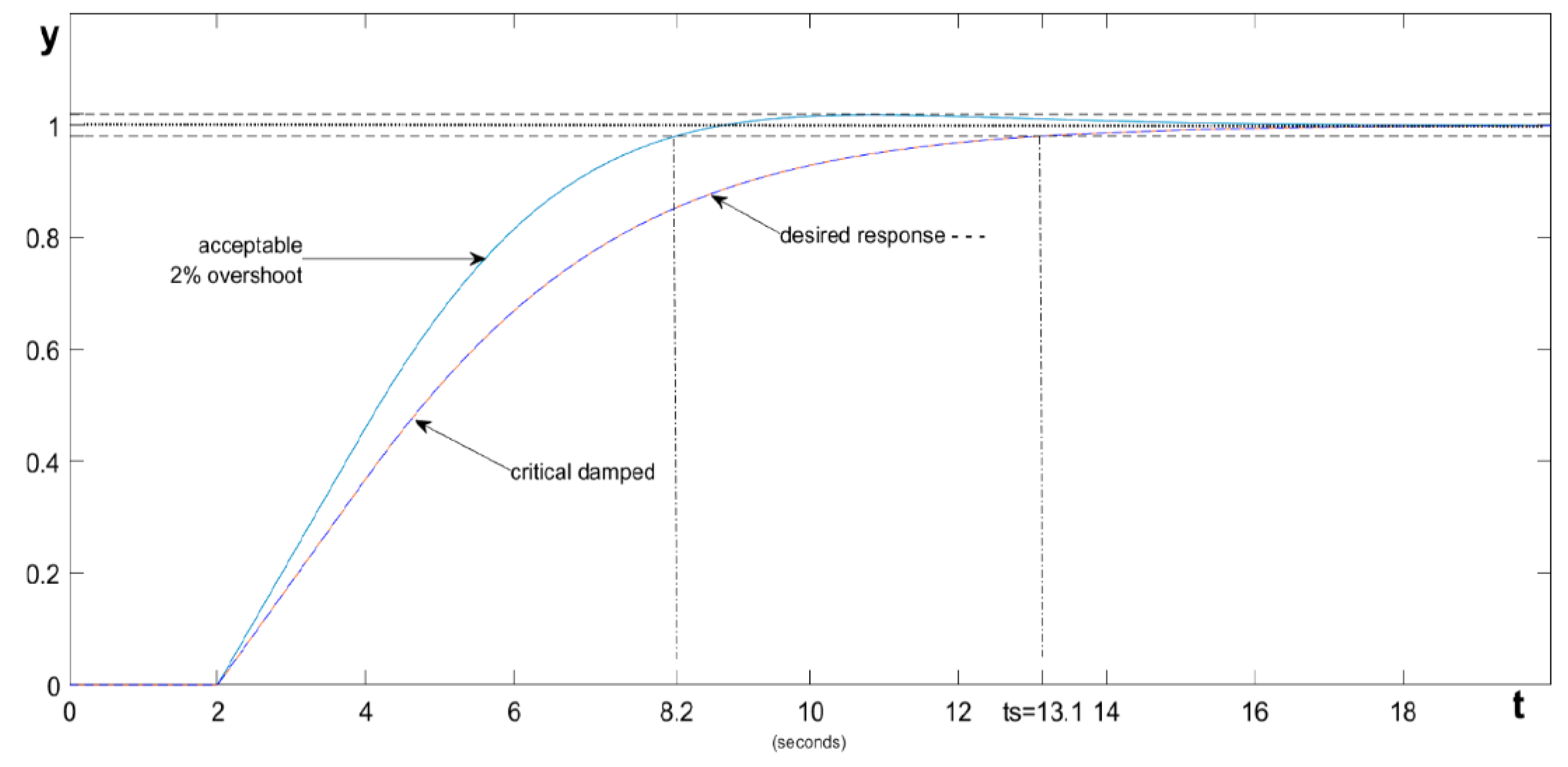
We have simulated this system, the results are shown in Figure B2. We have also calculated a controller that provides maximum speed with no overshoot, the result is shown in Figure B3.
Figure B2 confirms that our simulation results are consistent with the simulation results in [29], so the graphs obtained can be trusted. However, in the paper, the transient process with 5% overshoot provides a response time of 8.2 seconds, while the process without overshoot can only be obtained with a response time of 15 seconds. Our optimization gives a result with a response time of 9 seconds with an overshoot of less than 1%, and if no overshoot is required, our result, as shown in Figure B3, gives a response time of 10 seconds, which is 1.4 times better than the result in [29].
Conclusion 1. The article [29] presents a result which, in the opinion of its authors, is the best result with a PI controller that ensures the absence of overshoot. This statement is erroneous: we obtained a result with a better response speed by a factor of 1.4, with other PI controller coefficients.
The next example in the same article considers the problem of controlling an object with a transfer function of the following type:
This is also obviously a fictitious example. For this object, a PID controller with the following parameters is calculated: Kp = 1.101, Ti = 12 s, Td = 2.667 s. The PID controller equation is not found in this publication. Apparently, the authors did not provide it due to carelessness, but from the equations for closed systems, one can conclude that it is assumed to be in the following form:
The paper also gives the transient process for the object and the controller for this case, which is shown in Figure B2.
From Figure B5 it is evident that the PID controller, which the authors of the article [29] consider optimal for the object of example 2, i.e. for the object (B3), is far from optimal, since we obtained a PID controller for this object with which the duration of the transient process is 10 seconds versus 16 seconds with the controller from this article, and there is also no overshoot.
Conclusion 2. The article [29] presents a result which, in the opinion of its authors, is the best result with a PID controller that ensures the absence of overshoot. This statement is erroneous: we obtained a result with a better response speed by 1.6 times, with other PID controller coefficients.
The third example differs from the second example in that the coefficient in the second bracket in the denominator is taken equal to the coefficient in the first bracket, because of which the object model takes the following form:
In the article [29], a controller with the following parameters is calculated: Kp = 0.7358, Ti = 8 s, Td = 2 s and for this case, transient processes are given.
The authors of [29] then provide graphs showing how the transient process will change if the time constant in the object model changes by 20% up or down. When the time constant of the object model increases by 20%, overshoot occurs to a value of 11%, and when the time constant of the object decreases, the zone from the prescribed state changes from a value of 13.1 seconds to a value of 26.7 seconds. The corresponding graphs from this article [29] are shown in Figure B6. We simulated this system with the controller calculated in this article, the result is shown in Figure B7.
Conclusion 3. The article [29] presents a result that is refuted in some details by modeling. In particular, with an increased parameter, the overshoot is still less than stated in the article (7%, not 11%), but longer (it ends not after 25 seconds, but after 32 seconds). The processes also differ when this parameter is reduced. In addition, all three graphs are much more clearly inconsistent in the initial stage of the transient process: in the graphs from the article, they are very close to each other, and when modeled in the VisSim 5.0e software, these graphs diverge noticeably, and differ in the rate of increase.
The most interesting thing in this article happens further with the fourth and fifth examples. The fourth example is that the authors propose to replace the complex model with a simpler one, as shown in the fragment given in Figure B7.
Figure 7.
Fragment with the problem statement for example 4 from the publication [29].
Figure 7.
Fragment with the problem statement for example 4 from the publication [29].
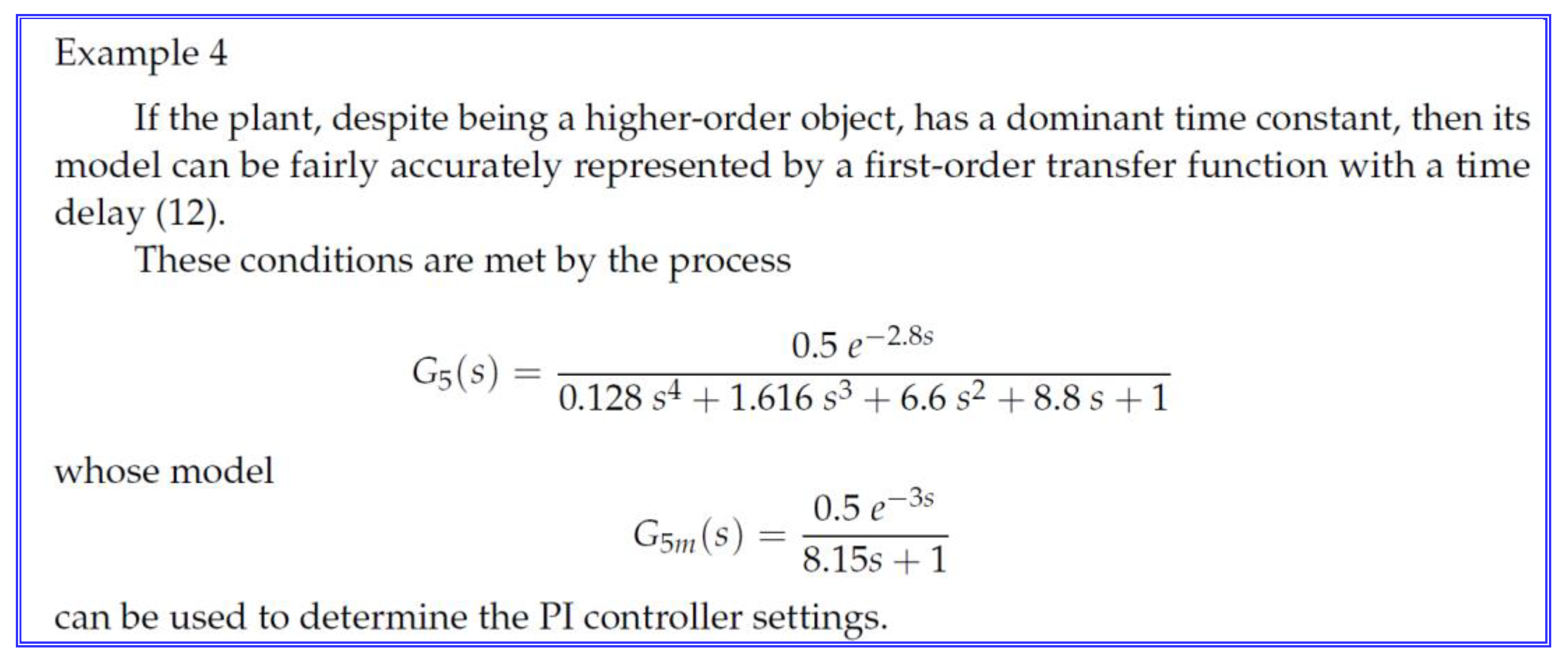
A natural question arises: to what extent is it permissible to replace a fourth-order model of an object with a first-order model? We believe that this is unacceptable if there are methods for using the exact model and if the exact model is known.
It is interesting that this article provides a comparison of the response graphs to a step jump of the object with the original transfer function and the model used for calculations. But this article does not contain a graph of the transient process in the resulting system, although the results of the PI controller calculation are provided. We will make up for this shortcoming. Firstly, the provided graphs of the comparison of transient processes are also unreliable. For comparison, we will provide these graphs side by side in Figure B8.
We see that in reality the lines are smoother, the duration of the process for the exact and approximate models on the left is about 40 seconds (we obtained it), while in the article it is twice as less, about 20 seconds, also in our modeling the graph of the exact model is always lower than the graph of the simplified model, while in the article these graphs intersect. From the left graphs it is clear that within the framework of the model used it is possible to find a more accurate approximation, from the right graphs it does not follow.
We believe that replacing the exact model with a simplified one is inappropriate for the reason that the authors of the article [29] in all cases set the task of finding a controller that would not have overshoot in the system. We calculated the controller for the simplified model and then applied the results of this calculation to the exact model. As a result, we obtained a system in which overshoot is about 8%. The corresponding graphs are shown in Figure B9.
Finally, the fifth example is taken from another publication [29], but judging by the model coefficients, this is also a fictitious example, and not an example taken from a practical problem, as shown in Figure B10.
We insist that approximating a fifth-order plant with a first-order model does not make sense. To prove this thesis, we calculated the controller using a simplified model and applied the results of this calculation to a system with an plant described by an exact model. The result is shown in Figure B11.
In this system, the overshoot is 25%, the transient process contains more than one oscillation wave. If the control problem was set without overshoot, then this example demonstrates that the problem is not solved. For comparison, we optimized the controller using an accurate model of the object. Figure B 12 shows the result. There is no overshoot in the system, the duration of the transient process is about 27 seconds. The article [58] presents a transient process with a duration of about 35 seconds, and the method for obtaining these transient process graphs still raises great doubts. Figure B13 shows the result of using the controller proposed in the article [29] to control the object from example 5, for which this controller is proposed. It is clear that the result is deplorable: the overshoot is 43%. The duration of the process is 240 seconds.
Conclusion 4. In the article [29], examples 4 and 5 present a method for calculating regulators using a simplified model of a complex object. This method is erroneous, since the calculation using a simplified model turns out to be unreliable (this statement is proven separately), and also for the reason that checking the functioning of the objects from these two examples with the regulators proposed in this article for these two examples shows that the transient processes in such systems differ greatly from the desired ones and differ from those given in this article.
Conclusion 5. The use of fictitious examples to demonstrate the operation of the method is acceptable, as it is used in other articles published by MDPI.
To avoid the impression that this conclusion was made based on a single article, we will give other examples. For example, in article [60], the simplest fictitious models of objects are also used to test the ideas put forward, as shown in Figure B 14. We will also give an example of article [61] and an illustrative example from it, shown as a fragment of the article in Figure B15.
Of course, mistakes in other people’s articles do not give us grounds to make mistakes in our own articles. However, the development of science should be based not only on each author striving to publish his own articles as soon as possible and as many as possible, but also on these articles being read by specialists in the field to which each article pertains. In addition, if a specialist sees an obvious mistake, he has the right to be surprised, and if a journal or publishing house allows for feedback from readers, then it is highly desirable that the errors found by readers be corrected by the editors in agreement with the authors or at their request. Moreover, it seems to us that if the mistake is obvious, then the authors of the article should be interested in correcting it.
In the paper [62], in equations (1) and (13), those factors that should be explicitly present as factors are moved so that they become part of the indices of the preceding quantities. Any specialist in this field will easily see this error. However, untrained readers will not realize that this is an error, and therefore will not understand what kind of relationship is given here. Of course, the reviewers should have seen this error.
In equation (1) it is written [62];
It should be written:
As we can see, there are two typos here: first, what should be a factor has turned into an index at “K”, and second, in this fragment “d” should be an index, and “s” should be a factor, which looks slightly different in the original.
In equation (13) it is written [62];
It should be written:
As we can see, two factors have turned into indices, and the index “I” (uppercase letter from “i”) in the second term has turned into “1” (a digit) or into “l” (lowercase letter from “L” if it is not written in italics). In addition, in the text, indices are repeatedly turned into factors, since they are written in the same register as the value itself. That is, the same values in the text are designated differently than in the formulas where these same values are used.
It is known that Albert Einstein also had typos in his early articles, but he always made sure that subsequent issues of these journals published corrections with apologies and corrected formulas [63]. Apparently, modern authors should also take care to correct typos and errors in their articles.
In another paper [64] an approximation of a ninth-order link by a first-order link is proposed.
The ninth-order model is given by equation (22), and the coefficients of this equation are given in Table 8. Model (23) is proposed as an approximation. Relation (23) is given in the following form:
An exponent to a numerical power is a number, not a function. In this case, there should be a transfer function of the delay link, where the module of the exponent indicates the magnitude of the delay, but at the same time, the variable “s” should be present in the exponent, since this is still a function, a model of the delay link, and not an ordinary number. Therefore, the following should be written:
In addition, it is quite obvious that the constant transfer coefficient of the model must coincide with the transfer coefficient of the link that is being modeled. The simplified model is represented by the relationship above, and the original mathematical model is designated as equation (23) and is represented by the following relationship:
In this case, Table 8 (numbering according to this article) gives the coefficients of this model, as shown in Figure B16.
When the ratio that the authors of the article [64] wanted to approximate becomes a simple fraction:
This is almost ten times more than it should be. So the coefficient in Table 8 should be at least ten times less, i.e. there is an extra zero after the decimal point. Obviously, it should be D0 = 0.587. However, even in this case, the coefficient should not be chosen equal to 5.1877, as stated in the article, but it should be equal to 5.11584327.
Accordingly, Figure 7 in this article is a fake. This figure is shown in Figure B17. This figure shows a surprisingly accurate match of the transient processes from the original exact model and from the proposed approximation for it. If we use the coefficients that are given in Table 8, then there will be no such match, but there will be a difference of about 10 times. There are still a number of shortcomings that can be pointed out in this article, but only the most obvious ones are listed here, which should have been noticed by absolutely any reviewer familiar with the field of knowledge for which this article is written. Our students know that checking the correctness of the model in the region of zero frequencies and in the region of infinite frequencies is a mandatory action when calculating regulators, and this is done in the mind, since it is very simple, you just need to divide one number by another.
In addition, the original model has a seventh-order polynomial in the numerator and a ninth-order polynomial in the denominator. In the high-frequency region, such a frequency characteristic of such a model tends to approach the asymptote corresponding to the second-order model. Therefore, it would be better to use a second-order model for approximation.
If scientific articles in high-ranking journals included in leading scientometric databases and having high impact factors at the level of Q1 – Q2 in these databases were not currently given such great importance in the entire global scientific community, then such typos and errors could be ignored.
We entered into correspondence with the publisher so that they would contact the authors of the article [64] for clarification. The authors admitted that in Table 8, in the value for the quantity, there is an extra zero after the decimal point. For some reason, the authors called this error a “typographical error”. The publication of an article does not include the typographical process, what the authors type on their computer is what will be published, so this is not a typographical error, but a typo made by the authors. However, no one is going to punish them for this typo, they are only asking them to correct this article! However, while admitting the error, they did not admit that it was made by them (although it could not be otherwise), indicating as the culprit a mysterious printing house employee who was not there, and at the same time did not promise to correct this typo, and did not correct it.
In text answer authors proposed such recognition: “In the exponent of the FOPDT model, the coefficient “s” should be present. I am sincerely regretting this minor typographical mistake. Hence, it is beyond any doubt that Figure 7 is a fake. The same can easily be obtained with the values given above. However, I am sincerely regretting two minor typographical mistakes, one in the coefficient of s0 in the numerator of (22), and another in the exponent of e in (23). I can understand that the minor typographical mistake in s0 of the numerator of (22) is creating some problem in understanding. This coefficient should be taken as 0.587, in place of 0.0587”.
At the time of writing, an uncorrected version of the article remains on the site. If the authors admitted that “Figure 7 is a fake,” why didn’t they correct the article? And why didn’t the editors of the journal make the corrections? If corrections had been made, we would not point out this misunderstanding. But if a scientific article can be edited to correct errors, or it can be provided with comments regarding errors, this should definitely be done if errors are present and even if they are acknowledged by the authors of the article.
With regard to checking the coincidence of the original characteristic with its model in the region of zero frequencies, that is, zero time, the authors responded with a strange phrase: “The value of K is chosen when the system is stabilized. This is the way to obtain the value of K. No one can run the simulation for infinite time». That is, the authors believe that in order to verify that the steady-state value of the transfer function in the zero-frequency region, in their opinion, it is necessary to run the simulation for an infinite time. Such an answer casts doubt on the competence of the authors, and this article was written by a team of four authors. It is surprising that each of the four authors should have read the article before agreeing to publish it in their own name, among other things. It is surprising that four authors and two reviewers did not notice these errors. But it is even more surprising that a team of four authors claims that in order to verify that the two transfer functions coincide in the zero-frequency region, it will be necessary to run the simulation for an infinite time, which no one can do.
Well then, we will do the work that no one else can do. Maybe we will be able to teach someone. First, let us recall that in order to find out what the transfer function of any link is in the zero frequency region, it is enough to substitute the value into it. We have already done this above. We hope that dividing one number by another is not so difficult that there is no excuse for not doing it. Now, let us present the simulation result, as shown in Figure B 18. If the authors had used the coefficients from Table 8, they would have obtained a result from which it is quite obvious that the graphs do not match; they differ by approximately 10 times. After adjusting the specified coefficient, the simulation can be repeated. The result is shown in Figure 19. This graph shows that simulating the process over a 30-second interval was enough to make sure that the static coefficients of the original transfer function and the model proposed for it do not significantly match.
Figure 18.
Graphs of the transient processes of the original transfer function and the model proposed for it from the publication [64], the red line is the process at the output of the exact model, the blue line is the process at the output of the approximating model.
Figure 18.
Graphs of the transient processes of the original transfer function and the model proposed for it from the publication [64], the red line is the process at the output of the exact model, the blue line is the process at the output of the approximating model.
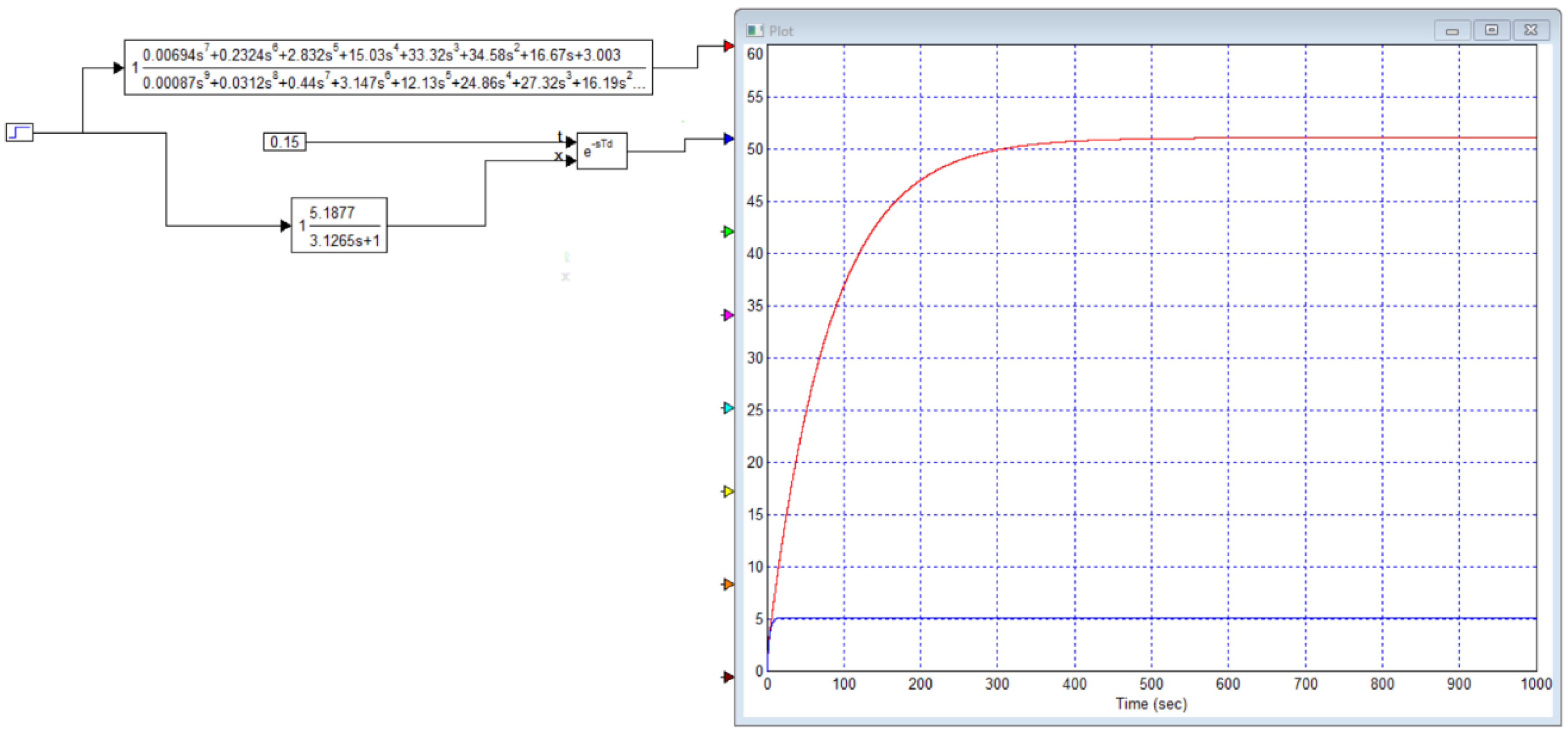
Figure 19.
Transient process graphs of the corrected initial transfer function and the model proposed for it from the publication [64], the red line is the process at the output of the exact model, the blue line is the process at the output of the approximating model: the discrepancy between the static coefficients is obvious; 30 seconds were enough for the simulation.
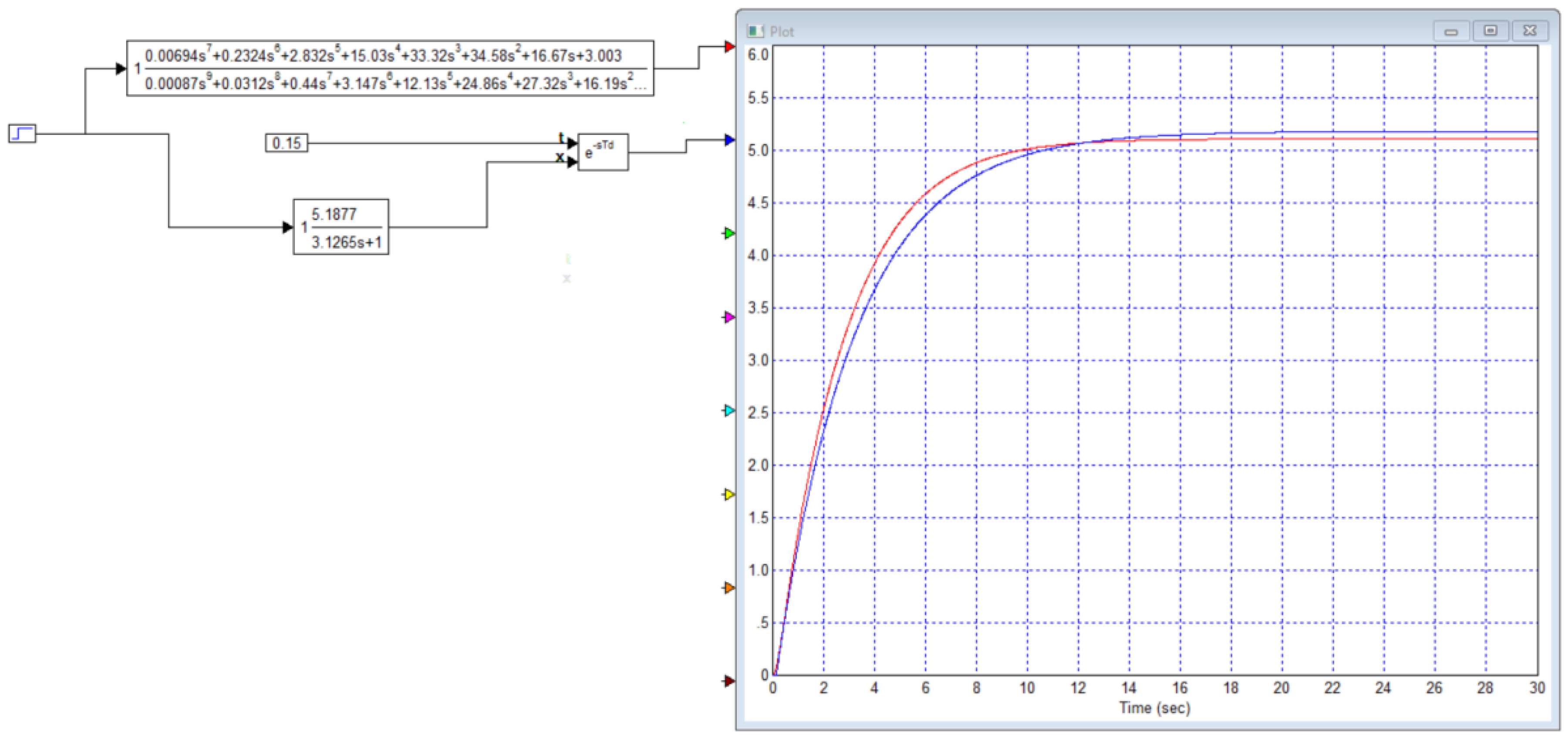
Figure 20.
Best approximation proposal: the red (exact) line is almost identical to the black one (our model proposal), and significantly different from the blue one (the approximation proposed in [64].
Figure 20.
Best approximation proposal: the red (exact) line is almost identical to the black one (our model proposal), and significantly different from the blue one (the approximation proposed in [64].
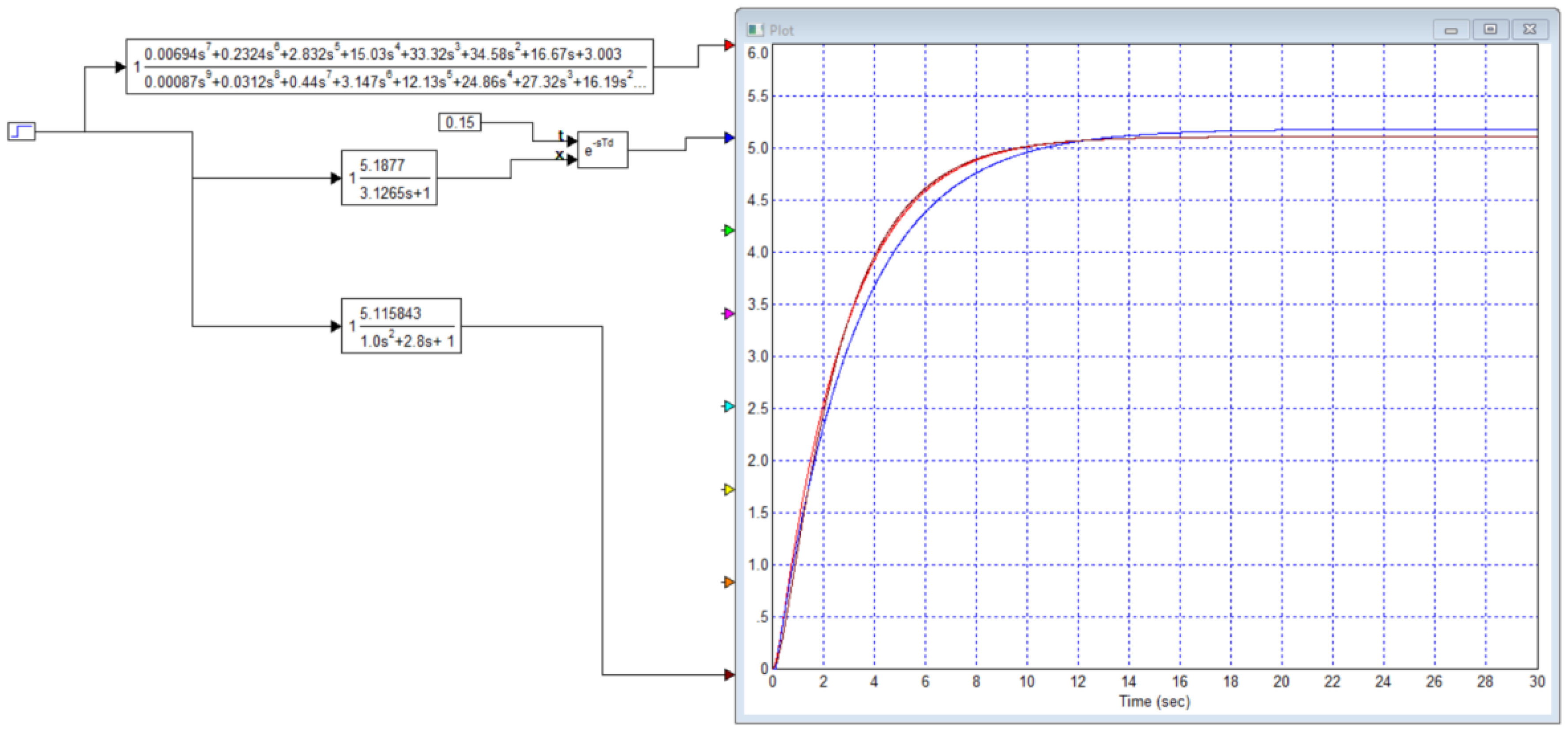
Figure 21.
Approximation error: blue line – approximation error proposed in the article, black line – approximation error obtained by manual selection based on the results of 15 tests (labor costs 10 minutes).
Figure 21.
Approximation error: blue line – approximation error proposed in the article, black line – approximation error obtained by manual selection based on the results of 15 tests (labor costs 10 minutes).
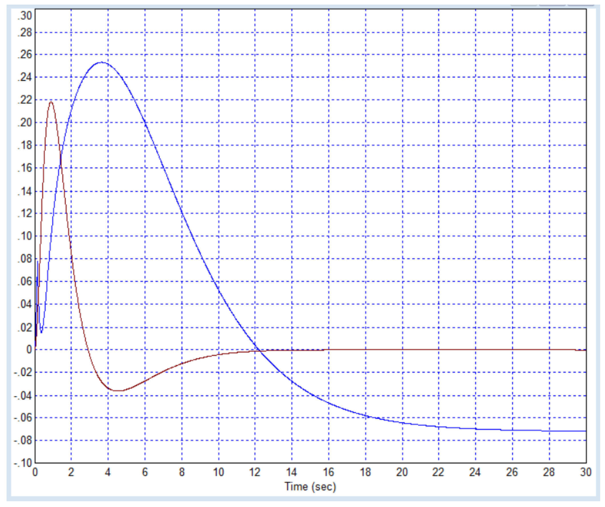
Conclusion 5. The method of numerical modeling and optimization is a simple and reliable tool, modeling with its help coincides with the results of reliable studies.
Conclusion 6. Numerical modeling allows us to identify errors in articles by other authors if they contain mathematical models of the object and the results of designing regulators.
Conclusion 7. In all cases, the controllers calculated using the numerical optimization method turn out to be better than the controllers published in the articles considered for the same objects.
Conclusion 8. The method of numerical optimization and numerical modeling is extremely easy to use, testing the main hypotheses takes little time, and the result is quite clear.
Numerical optimization has been used to calculate many controllers for practical and educational tasks. In particular, postgraduate student A. Yu. Ivoylov and senior lecturer V. G. Trubin designed and manufactured a compact balancing robot. The video at the link [65] demonstrates the operation of two versions of this robot [66,67]. The robot on the left maintains balance, but makes some deviations around the equilibrium state. The robot on the right maintains balance without deviations, which is ensured by optimizing the PID controller under the supervision of one of the authors of this article.
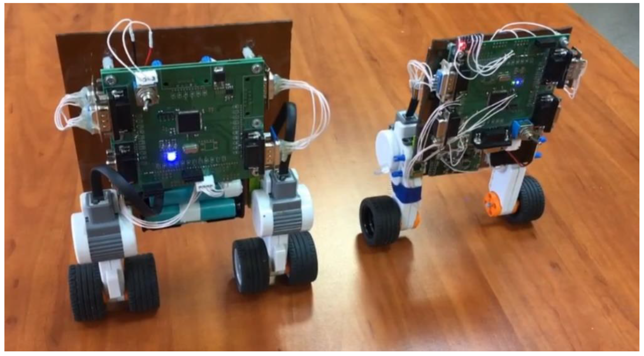
References
- Konkov, A. E. ; Mitrishkin, YV Synthesis Methodology for Discrete MIMO PID Controller with Loop Shaping on LTV Plant Model via Iterated LMI Restrictions. Mathematics 2024, 12, 810. [Google Scholar] [CrossRef]
- Krokavec, D.; Filasová, A. On PID Design Constraints in Relation to Control of Strictly Metzler Linear MIMO Systems. Symmetry 2021, 13, 1589. [Google Scholar] [CrossRef]
- Guo, X.; Shirkhani, M.; Ahmed, E.M. Machine-Learning-Based Improved Smith Predictive Control for MIMO Processes. Mathematics 2022, 10, 3696. [Google Scholar] [CrossRef]
- Almeida, A.Md. ; Daga, AL; Lanzarini, RPSP; Lenzi, E. K.; Lenzi, MK High-Performance Identification and Control of MIMO (Multiple Input—Multiple Output) Experimental Module with Fractional-Order Approach Application. Fractal Fracture. 2025, 9, 226. [Google Scholar] [CrossRef]
- Garrido, J.; Garrido-Jurado, S.; Vázquez, F.; Arrieta, O. Design of Multivariable PID Control Using Iterative Linear Programming and Decoupling. Electronics 2024, 13, 698. [Google Scholar] [CrossRef]
- Peretz, Y. A Randomized Algorithm for Optimal PID Controllers. Algorithms 2018, 11, 81. [Google Scholar] [CrossRef]
- Afifa, R.; Ali, S.; Pervaiz, M.; Iqbal, J. Adaptive Backstepping Integral Sliding Mode Control of a MIMO Separately Excited DC Motor. Robotics 2023, 12, 105. [Google Scholar] [CrossRef]
- Piñon, A.; Favela-Contreras, A.; Beltran-Carbajal, F.; Lozoya, C.; Dieck - Assad, G. Novel Strategy of Adaptive Predictive Control Based on a MIMO-ARX Model. Actuators 2022, 11, 21. [Google Scholar] [CrossRef]
- La, H.; Oh, K. Development of a Universal Adaptive Control Algorithm for an Unknown MIMO System Using Recursive Least Squares and Parameter Self-Tuning. Actuators 2024, 13, 167. [Google Scholar] [CrossRef]
- Kato, T.; Nishizawa, K.; Deng, M. MSVR & Operator-Based System Design of Intelligent MIMO Sensorless Control for Microreactor Devices. Computation 2024, 12, 2. [Google Scholar] [CrossRef]
- Formalization of requirements for locked-loop control systems for their numerical optimization / VA Zhmud, GA Frantsuzova, L. Dimitrov, J. Nosek // Recent research in control engineering and decision making. – Springer Intern. Publ., 2019. – P. 353-365. - (Systems, Decision and Control; vol. 199). ISBN 978-3-030-12072-6. [CrossRef]
- Zhmud, V.; Dimitrov, L. Using the Fractional Differential Equation for the Control of Objects with Delay. Symmetry 2022, 14, 635. [Google Scholar] [CrossRef]
- Baar, T.; Bauer, P.; Luspay, T. Parameter Varying Mode Decoupling for LPV systems. IFAC- PapersOnLine 2020, 53, 1219–1224. [Google Scholar] [CrossRef]
- Feng, Z. Y.; Guo, H.; She, J.; Xu, L. Weighted sensitivity design of multivariable PID controllers via a new iterative LMI approach. J. Process Control 2022, 110, 24–34. [Google Scholar] [CrossRef]
- Guo, H.; Feng, Z. Y.; She, J. Discrete-time multivariable PID controller design with application to an overhead crane. Int. J. Syst. Sci. 2020, 51, 2733–2745. [Google Scholar] [CrossRef]
- Solgi, Y.; Fatehi, A.; Nikoofard, A.; Shariati, A. Design of optimal PID controller for multivariable time-varying delay discrete-time systems using non-monotonic Lyapunov-Krasovskii approach. J. Frankl. Inst. 2021, 358, 6634–6665. [Google Scholar] [CrossRef]
- Zhmud VA The method of correct calculation of regulators based on numerical optimization / VA Zhmud, LV Dimitrov // Journal of Physics: Conference Series. - 2019. - Vol. 1210. - Art. 012168 (10 p.). -. [CrossRef]
- VA Zhmud, LV Dimitrov. The influence of the type of the test signal on the result of numerical optimization of regulators. Journal of Physics; Conference Series. - 2017. - Vol. 803. - Art. 012186 (6 p.). -. [CrossRef]
- Konkov, A. E. ; Mitrishkin, YV; Korenev, PS; Patrov, MI Robust Cascade LMI Design of MIMO Control System for Plasma Position, Current, and Shape Model with Time-Varying Parameters in a Tokamak. IFAC- PapersOnLine 2020, 53, 7344–7349. [Google Scholar] [CrossRef]
- Mitrishkin, YV; Korenev, PS; Konkov, A. E.; Kartsev, N.M. Suppression of Vertical Plasma Displacements by Control System of Plasma Unstable Vertical Position in D-Shaped Tokamak. Autom. Remote Control 2022, 83, 579–599.
- Konkov, A. E. ; Mitrishkin, YV Comparison Study of Power Supplies in Real-Time Robust Control Systems of Vertical Plasma Position in Tokamak. IFAC- PapersOnLine 2022, 55, 327–332. [Google Scholar] [CrossRef]
- Konkov, A. E. ; Korenev, PS; Mitrishkin, YV; Balachenkov, I. M.; Kiselev, EO Real-Time Plasma Magnetic Control System with Equilibrium Reconstruction Algorithm in the Feedback for the Globus-M2 Tokamak. Plasma Phys. Rep. 2023, 49, 1552–1559. [Google Scholar]
- Krokavec, D.; Filasová, A. PID control design for SISO strictly Metzlerian linear systems. Symmetry 2020, 12, 1979. [Google Scholar] [CrossRef]
- Tsavnin, A.; Efimov, S.; Zamyatin, S. Overshoot elimination for control systems with parametric uncertainty via a PID controller. Symmetry 2020, 12, 1092. [Google Scholar] [CrossRef]
- Zhang, W.; Cui, Y.; Ding, X. An improved analytical tuning rule of a robust PID controller for integrating systems with time delay based on the multiple dominant pole-placement method. Symmetry 2020, 12, 1449. [Google Scholar] [CrossRef]
- An, Q.; Guo, H.; Zheng, Y. On Robust Stability and Stabilization of Networked Evolutionary Games with Time Delays. Mathematics 2022, 10, 2695. [Google Scholar] [CrossRef]
- Liu, X.; Li, W.; Yao, C.; Li, Y. Finite-Time Guaranteed Cost Control for Markovian Jump Systems with Time-Varying Delays. Mathematics 2022, 10, 2028. [Google Scholar] [CrossRef]
- Tavoosi, J.; Shirkhani, M.; Abdali, A.; Mohammadzadeh, A.; Nazari, M.; Mobayen, S.; Asad, J. H.; Bartoszewicz, A. A New General Type-2 Fuzzy Predictive Scheme for PID Tuning. Appl. Sci. 2021, 11, 10392. [Google Scholar] [CrossRef]
- Panda, R. C. ; Yu, CC; Huang, H. -P. PID tuning rules for SOPDT systems: Review and some new results. ISA Trans. 2004, 43, 283–295. [Google Scholar]
- Euzébio, T.A. ; Yamashita, AS; Pinto, TV; Barros, PR SISO approaches for linear programming based methods for tuning decentralized PID controllers. J. Process Control. 2020, 94, 75–96. [Google Scholar] [CrossRef]
- Garrido, J.; Ruz, M.L.; Morilla, F.; Vázquez, F. Iterative Method for Tuning Multiloop PID Controllers Based on Single Loop Robustness Specifications in the Frequency Domain. Processes 2021, 9, 140. [Google Scholar] [CrossRef]
- Carlucho, I.; De Paula, M.; Acosta, G.G. An adaptive deep reinforcement learning approach for MIMO PID control of mobile robots. ISA Trans. 2020, 102, 280–294. [Google Scholar] [CrossRef]
- Veerasamy, V. ; Wahab, NIA; Ramachandran, R. ; Othman, M.L.; Hizam, H.; Kumar, JS; Irudayaraj, AXR Design of single-and multi-loop self-adaptive PID controller using heuristic based recurrent neural network for ALFC of hybrid power system. Expert Syst. Appl. 2022, 192, 116402. [Google Scholar]
- de Almeida, A. M.; Lenzi, M.K. ; Lenzi, EK Decentralized fractional-order PI λ control applied to a TITO distillation column: A comparative study with PID and MPC. Cuad. Educ. Desarollo 2024, 16, e6021. [Google Scholar] [CrossRef]
- Edet, E. B.; Chacón-Vásquez, M. ; Onyeocha, EC Application of Fractional-order PID controllers in a Greenhouse Climate Control System. IFAC- PapersOnLine 2024, 58, 179–184. [Google Scholar] [CrossRef]
- Martínez-Luzuriaga, P.N.; Reynoso-Meza, G. Influencia de Los Hiper-Parámetros En Algoritmos Basados En Evolución Diferencial Para El Ajuste de Controladores del tipo PID en Procesos SISO. Rev. Iberoam. De Automática E Informática Ind. 2023, 20, 44–55. [Google Scholar] [CrossRef]
- Rojas, J.D.; Arrieta, O.; Vilanova, R. Industrial PID Controller Tuning with a Multiobjective Framework Using MATLAB®, 1st ed.; Springer: Cham, Swizterland, 2022; ISBN 978-3-030-72313-2. [Google Scholar]
- Jeng, J.C. ; Lee, MW Multi-Loop PID Controllers Design with Reduced Loop Interactions Based on a Frequency-Domain Direct Synthesis Method. J. Frankl. Inst. 2023, 360, 2476–2506. [Google Scholar] [CrossRef]
- Mahapatro, S.R.; Subudhi, B. A New Hinf Weighted Sensitive Function Based Robust Multi-Loop PID Controller for a Multi-Variable System. IEEE Trans. Circuits Syst. II Express Briefs, 2023; early access.
- Mahapatro, S.R.; Subudhi, B. A Robust Decentralized PID Controller Based on Complementary Sensitivity Function for a Multivariable System. IEEE Trans. Circuits Syst. II Express Briefs 2020, 67, 2024–2028. [Google Scholar] [CrossRef]
- Euzebio, T.A.M.; Da Silva, M.T. ; Yamashita, AS Decentralized PID Controller Tuning Based on Nonlinear Optimization to Minimize the Disturbance Effects in Coupled Loops. IEEE Access 2021, 9, 156857–156867. [Google Scholar] [CrossRef]
- Euzébio, T.A.M. ; Yamashita, AS; Pinto, TVB; Barros, PR SISO Approaches for Linear Programming Based Methods for Tuning Decentralized PID Controllers. J. Process Control 2020, 94, 75–96. [Google Scholar] [CrossRef]
- Garrido, J.; Ruz, M.L.; Morilla, F.; Vázquez, F. Iterative Method for Tuning Multiloop Pid Controllers Based on Single Loop Robustness Specifications in the Frequency Domain. Processes 2021, 9, 140. [Google Scholar] [CrossRef]
- Garrido, J.; Ruz, M.L.; Morilla, F.; Vázquez, F. Iterative Design of Centralized PID Controllers Based on Equivalent Loop Transfer Functions and Linear Programming. IEEE Access 2022, 10, 1440–1450. [Google Scholar] [CrossRef]
- Feng, Z. Y.; Guo, H.; She, J.; Xu, L. Weighted Sensitivity Design of Multivariable PID Controllers via a New Iterative LMI Approach. J. Process Control 2022, 110, 24–34. [Google Scholar] [CrossRef]
- Da Silva, M.T. ; Barros, PR An Iterative Procedure for Tuning Decentralized PID Controllers Based on Effective Open-Loop Process. In Proceedings of the 7th International Conference on Control, Decision and Information Technologies, CoDIT 2020, Prague, Czech Republic, 29 June–2 July 2020; pp. 813–818. [Google Scholar]
- Pongfai, J.; Angeli, C.; Shi, P.; Su, X.; Assawinchaichote, W. Optimal PID controller autotuning design for MIMO nonlinear systems based on the adaptive SLP algorithm. Int. J. Control Autom. Syst. 2021, 19, 392–403. [Google Scholar] [CrossRef]
- 21–22 October 2022, Tajudin, AI; Izani, M.A.D.; Samat, AAA; Omar, S.; Idin, MAM Design a speed control for DC motor using an optimal PID controller implementation of ABC algorithm. In Proceedings of the IEEE 12th International Conference on Control System, Computing and Engineering (ICCSCE), Penang, Malaysia, ; pp. 97–102.
- Li, F.; Yang, L.; Ye, A.; Zhao, Z.; Shen, B. Grouping Neural Network-Based Smith PID Temperature Controller for Multi-Channel Interaction System. Electronics 2024, 13, 697. [Google Scholar] [CrossRef]
- Liu, Z.; Liu, Z.; Liu, J.; Wang, N. Thermal management with fast temperature convergence based on optimized fuzzy PID algorithm for electric vehicle battery. Appl. Energy 2023, 352, 121936. [Google Scholar] [CrossRef]
- Han, S.Y.; Dong, J. F.; Zhou, J.; Chen, Y. H. Adaptive Fuzzy PID Control Strategy for Vehicle Active Suspension Based on Road Evaluation. Electronics 2022, 11, 921. [Google Scholar] [CrossRef]
- Abdelwanis, MI; El- Sousy, FFM; Ali, M. M. A Fuzzy-Based Proportional Integral Derivative with Space-Vector Control and Direct Thrust Control for a Linear Induction Motor. Electronics 2023, 12, 4955.
- Ding, Y.; Ren, X.; Zhang, X.; Liu, X.; Wang, X. Multi-Phase Focused PID Adaptive Tuning with Reinforcement Learning. Electronics 2023, 12, 3925. [Google Scholar] [CrossRef]
- Gopmandal, F.; Ghosh, A. LQR-based MIMO PID control of a 2-DOF helicopter system with uncertain cross-coupled gain. IFAC- PapersOnLine 2022, 55, 183–188. [Google Scholar] [CrossRef]
- Carlucho, I.; De Paula, M.; Acosta, G.G. An adaptive deep reinforcement learning approach for MIMO PID control of mobile robots. ISA Trans. 2020, 102, 280–294. [Google Scholar] [CrossRef]
- Sagar, JD DC Motor Control using PID Controller. Int. Res. J. Eng. Technol. 2020, 7, 1765–1769.
- Wati, T. ; Subiyanto; Sutarno. Simulation model of speed control DC motor using fractional order PID controller. J. Phys. Conf. Ser. 2020, 1444, 012022. [Google Scholar]
- Zhmud, V. Controlling of Multichannel Objects with Non-Square Transfer Function. Automation 2025, 6, 27. [Google Scholar] [CrossRef]
- Kula, KS Tuning a PI/PID Controller with Direct Synthesis to Obtain a Non-Oscillatory Response of Time-Delayed Systems. Appl. Sci. 2024, 14, 5468. [CrossRef]
- Ding, Y.; Ren, X.; Zhang, X.; Liu, X.; Wang, X. Multi-Phase Focused PID Adaptive Tuning with Reinforcement Learning. Electronics 2023, 12, 3925. [Google Scholar] [CrossRef]
- Kos, T.; Huba, M.; Vrančić, D. Parametric and Nonparametric PI Controller Tuning Method for Integrating Processes Based on Magnitude Optimum. Appl. Sci. 2020, 10, 1443. [Google Scholar] [CrossRef]
- Al-Dhaifallah, M. Construction and Evaluation of a Control Mechanism for Fuzzy Fractional-Order PID. Appl. Sci. 2022, 12, 6832. [Google Scholar] [CrossRef]
- Correcting Publisher’s Errors in Einstein’s “Relativity”. https://manuelgarciajr. 2015.
- Bashishtha, TK; Singh, V. P.; Yadav, UK; Varshney, T. Reaction Curve-Assisted Rule-Based PID Control Design for Islanded Microgrid. Energies 2024, 17, 1110. [CrossRef]
- https://kb-au.ru/wp-content/uploads/NSTU-PLATF2_3-2018.
- Suppression of oscillations of a two-wheeled balancing robot / VA Zhmud, LV Dimitrov, OV Stukach, AY Ivoilov, H. Roth, GV Sablina // Dynamics of systems, mechanisms and machines (DYNAMICS); proc., 13 intern. sci. and techn. conf., Omsk, 5–7 Nov. 2019. – IEEE, 2019. – 5 p. https://ieeexplore.ieee.org/stamp/stamp.jsp?tp=&arnumber=8944728. ISBN 978-1-7281-0970-1. -. [CrossRef]
- Parametric Synthesis of the Control System of the Balancing Robot by the Numerical Optimization Method / A.Y. Ivoilov, V.A. Parametric Synthesis of the Control System of the Balancing Robot by the Numerical Optimization Method / A.Y. Ivoilov, V.A. Zhmud, V.G. Trubin, H. Roth. Mekhatronika, avtomatizatsiya, upravlenie. - 2019. - No. 6. - P. 352-361. -. [CrossRef]
Figure 1.
Traditional structure of a negative feedback system.
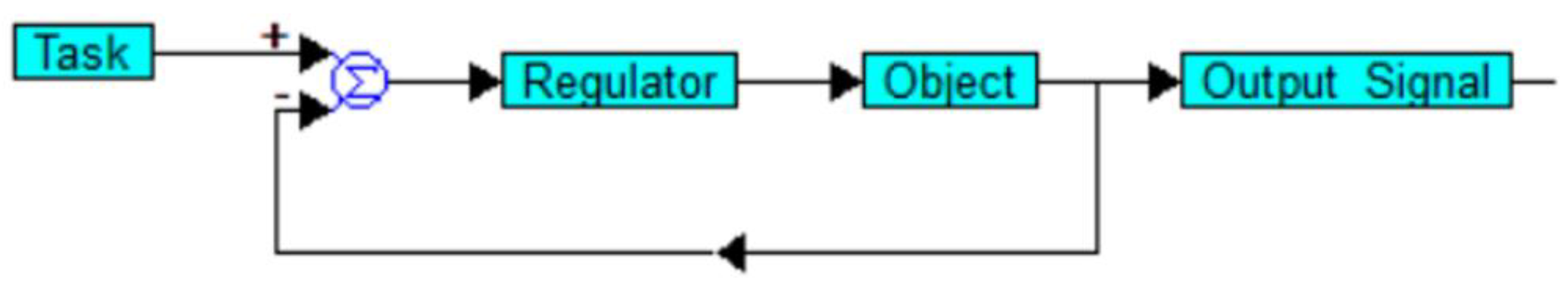
Figure 2.
Example 1 of object.
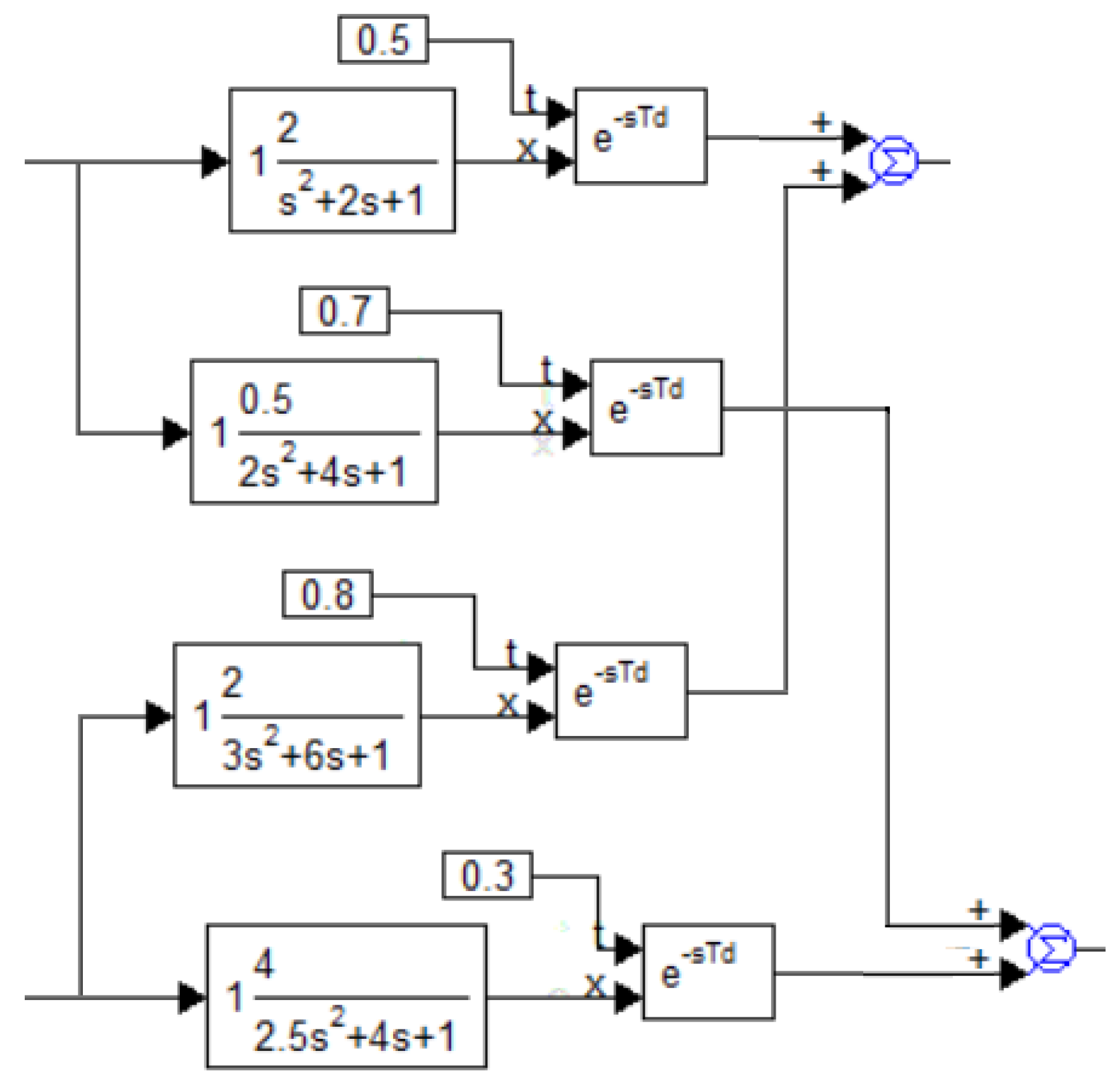
Figure 3.
Project and result of optimization of the system with the object according to example 1.
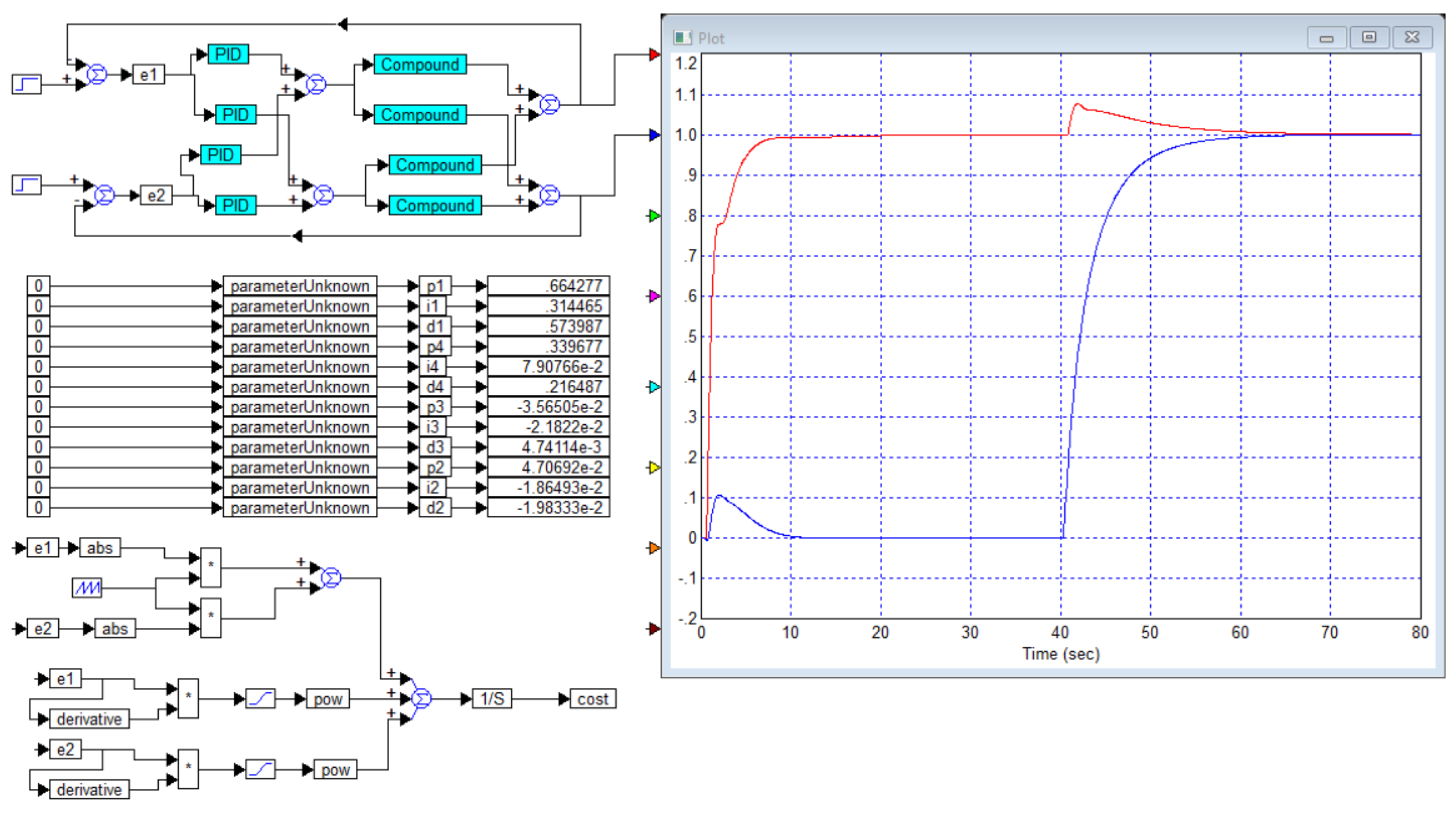
Figure 4.
Project for solving Example 1 using a diagonal PID controller, i.e. actually two scalar controllers, as well as the obtained result: controller coefficients and transient process graphs.
Figure 4.
Project for solving Example 1 using a diagonal PID controller, i.e. actually two scalar controllers, as well as the obtained result: controller coefficients and transient process graphs.
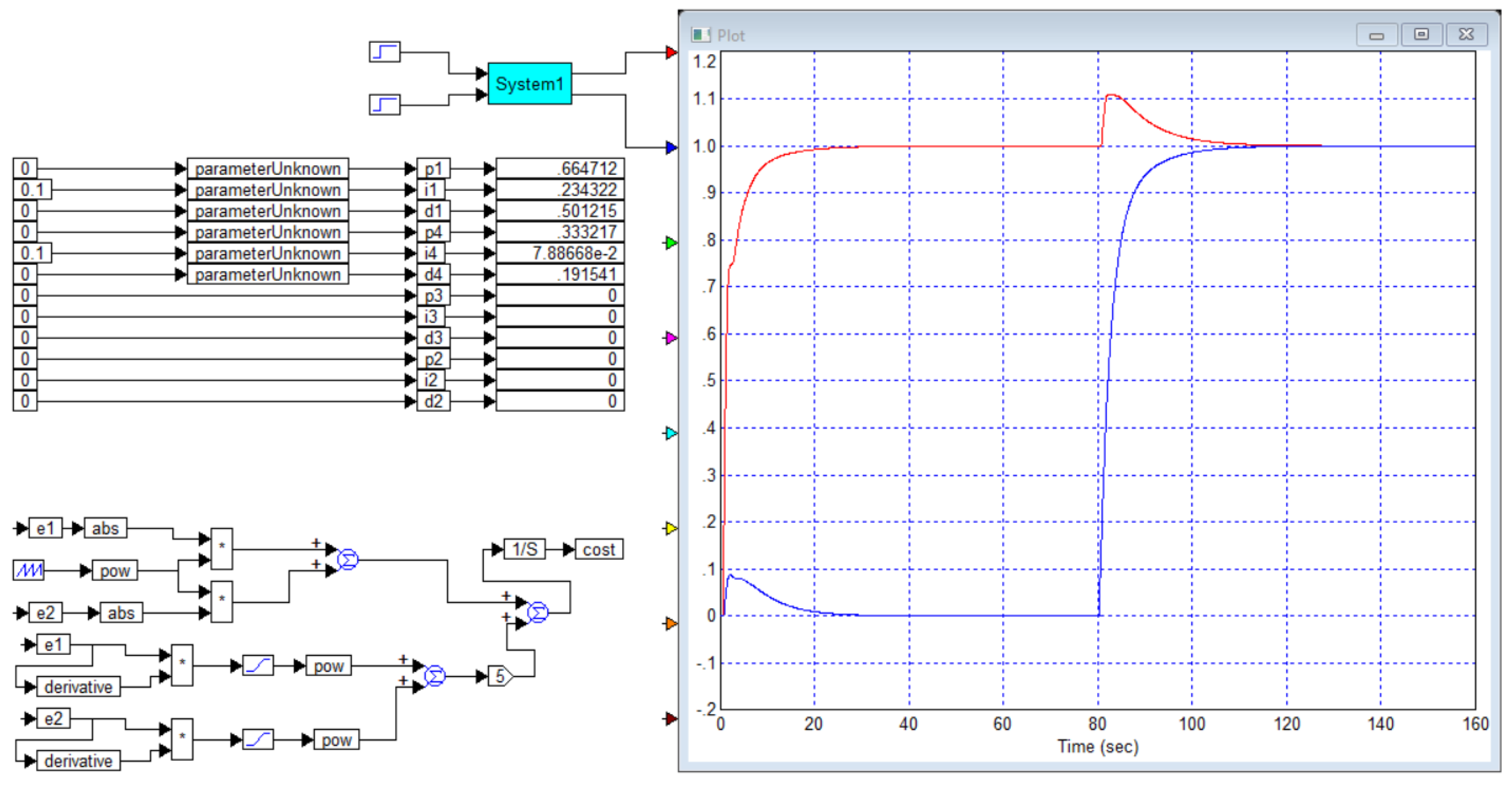
Figure 5.
Result of attempt to optimize the diagonal regulator controller for the Example 2 object: the system turned out to be unstable.
Figure 5.
Result of attempt to optimize the diagonal regulator controller for the Example 2 object: the system turned out to be unstable.
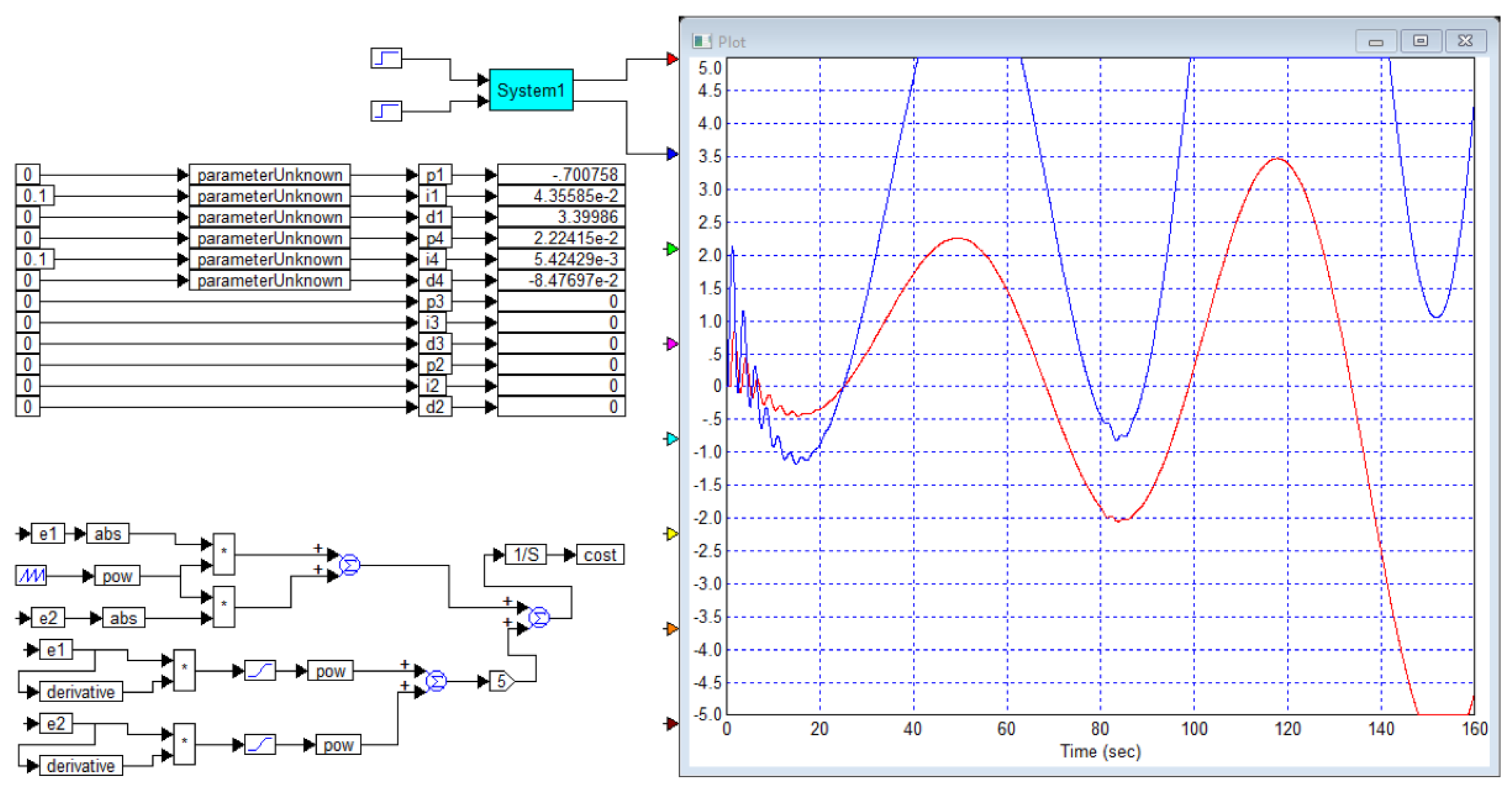
Figure 6.
Project and result of an attempt to calculate a full matrix PID controller for the same object from Example 2: a stable system was obtained.
Figure 6.
Project and result of an attempt to calculate a full matrix PID controller for the same object from Example 2: a stable system was obtained.
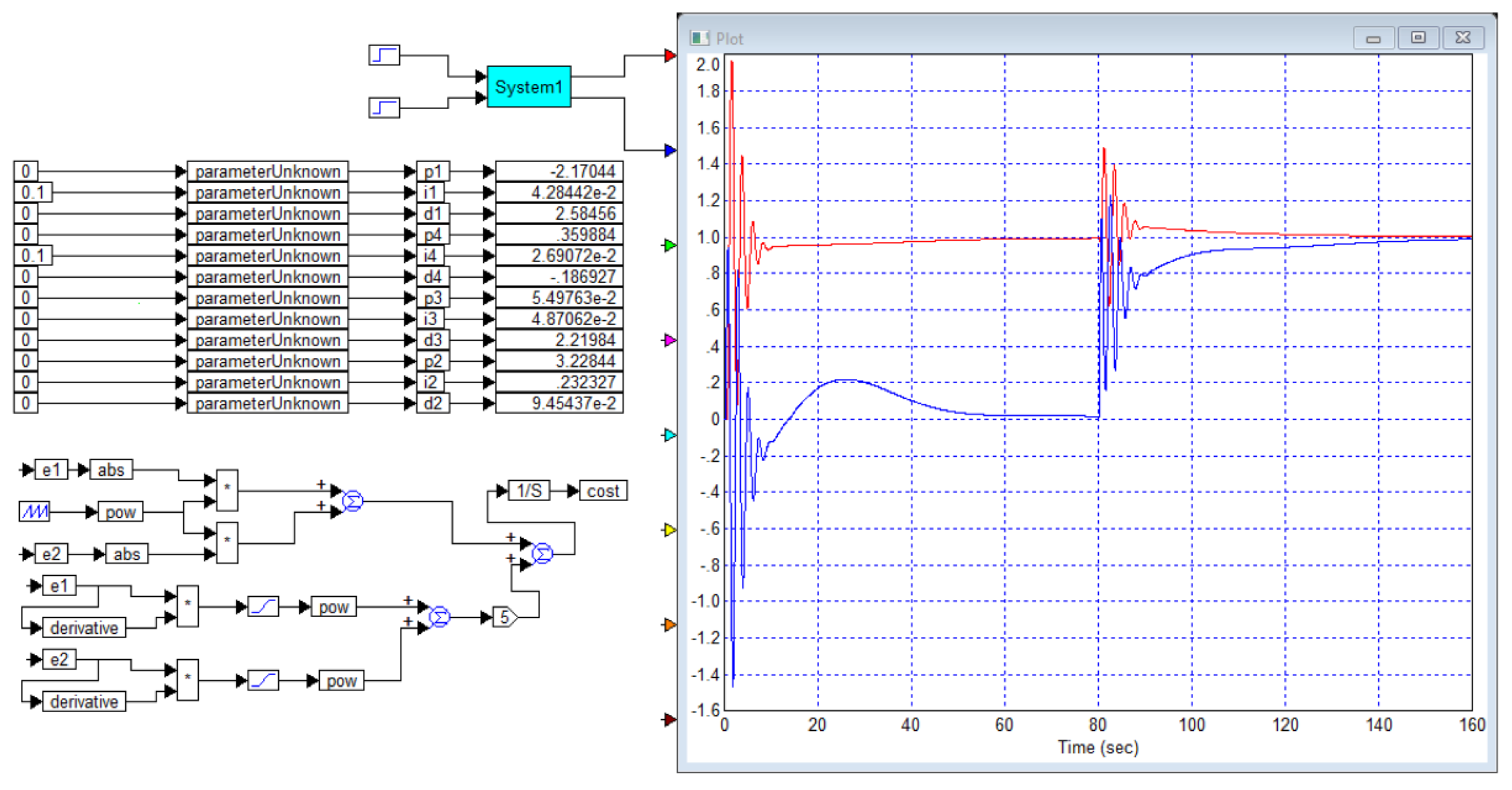
Figure 7.
Result of designing and optimizing the full PID controller for the object from example 3: the system is stable, but the response of the second channel to a jump in the setpoint the first channel is too big.
Figure 7.
Result of designing and optimizing the full PID controller for the object from example 3: the system is stable, but the response of the second channel to a jump in the setpoint the first channel is too big.
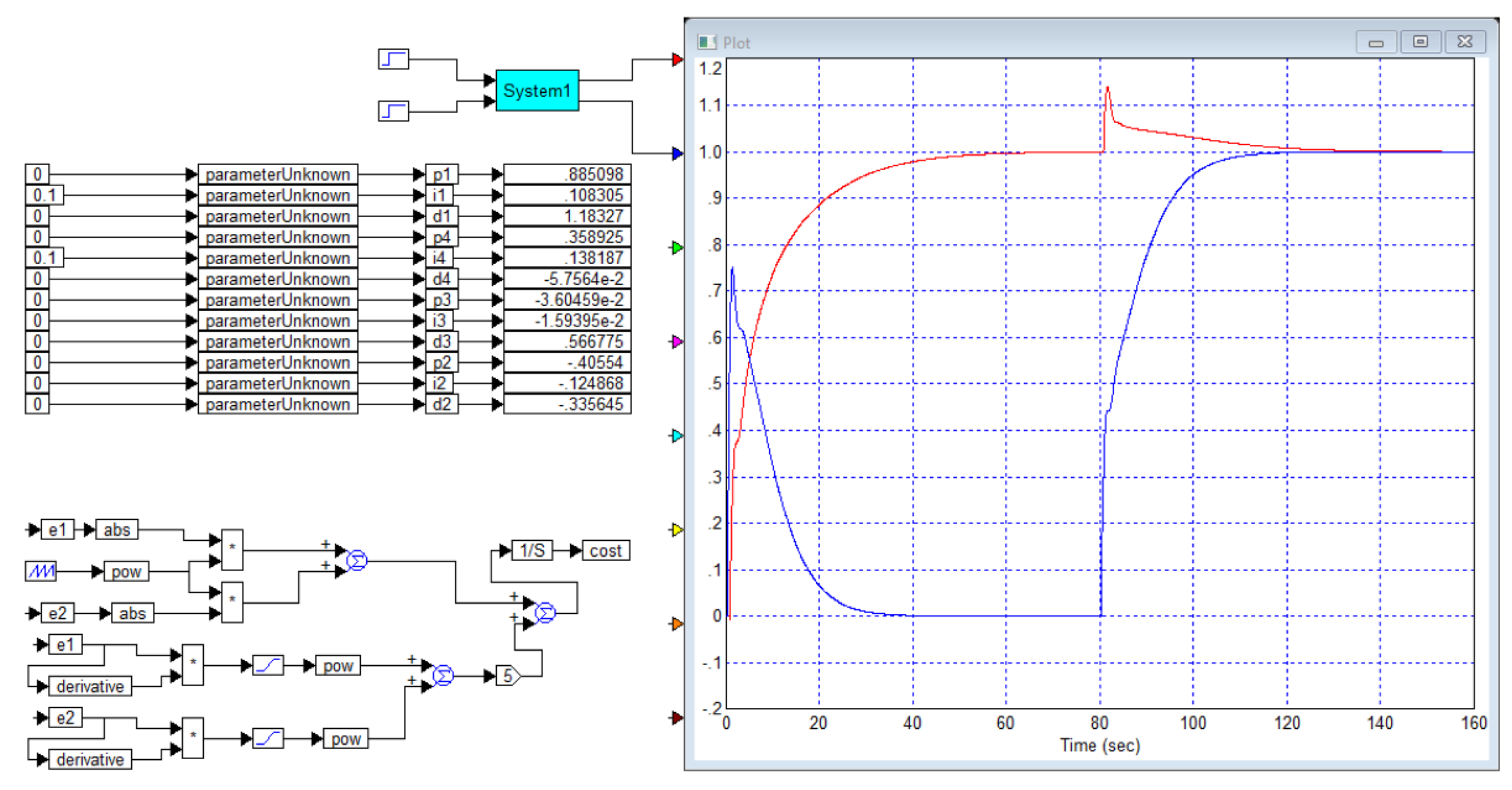
Figure 8.
Project and result of controlling the object of example 3 using a diagonal regulator.
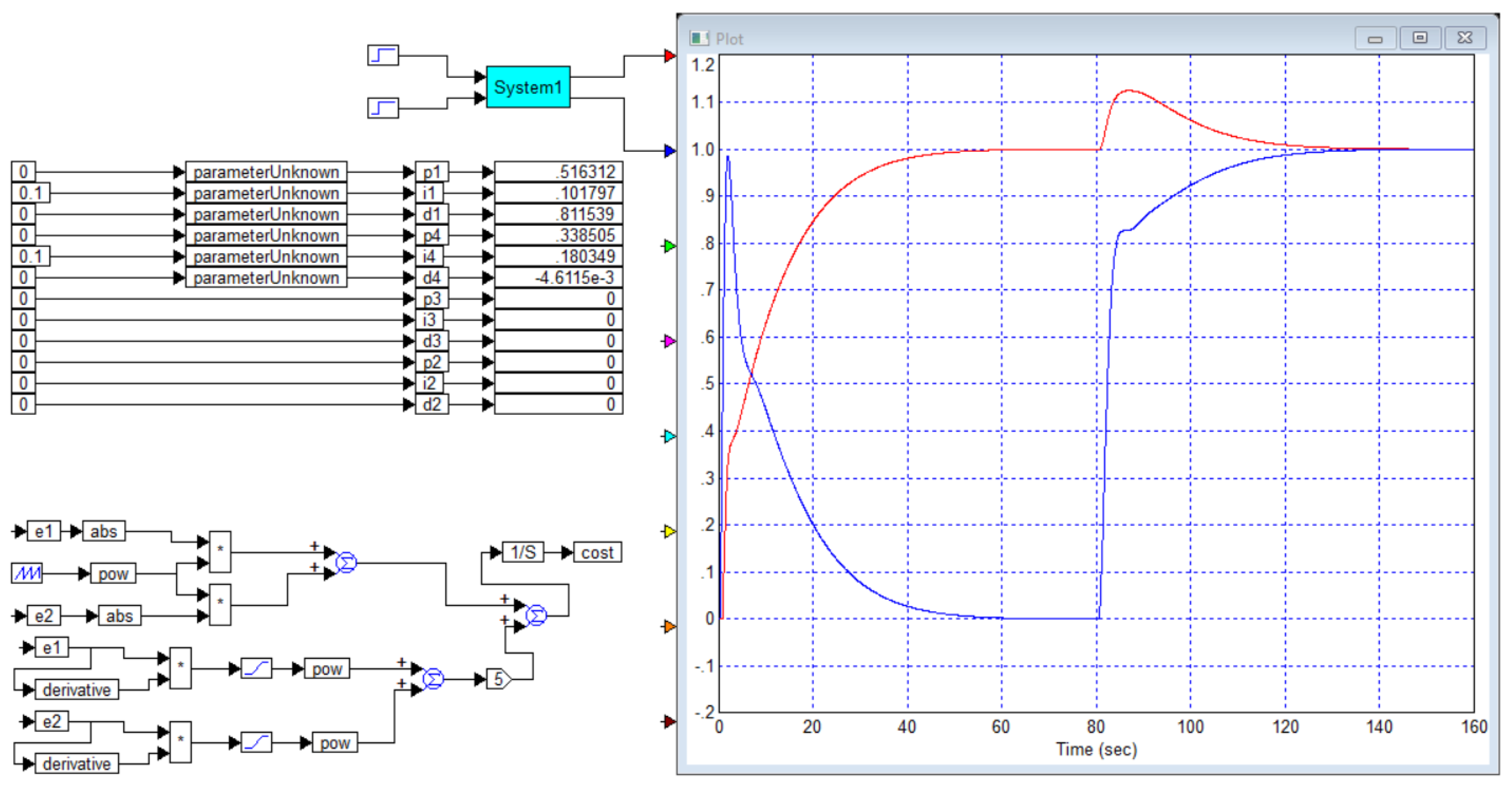
Figure 9.
Result of design and optimization of the diagonal controller for example 4.
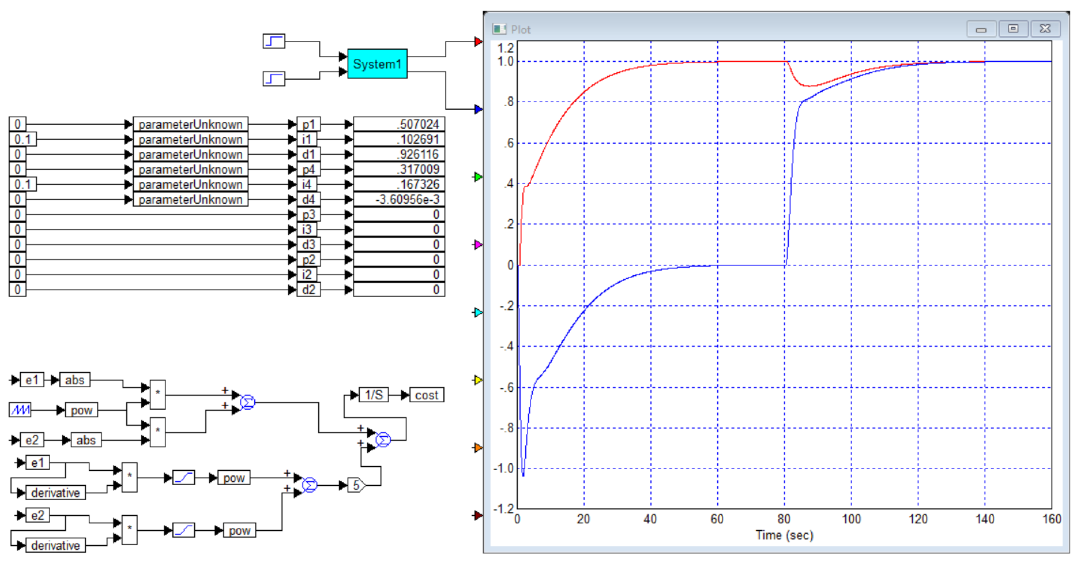
Figure 10.
Result of designing and optimizing a complete controller for the object from example 4.
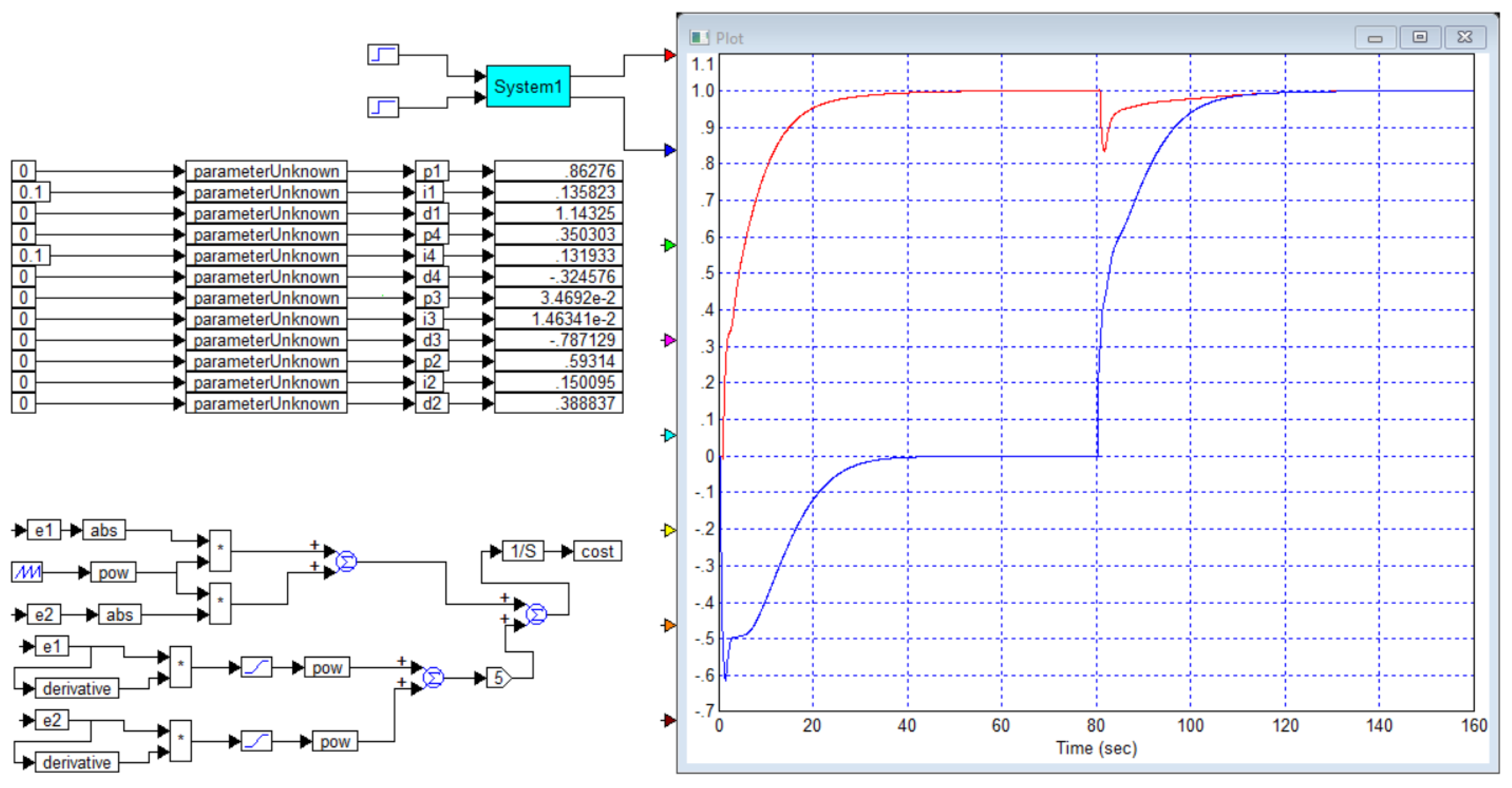
Figure 11.
Design and result of numerical optimization of the controller for example 5.
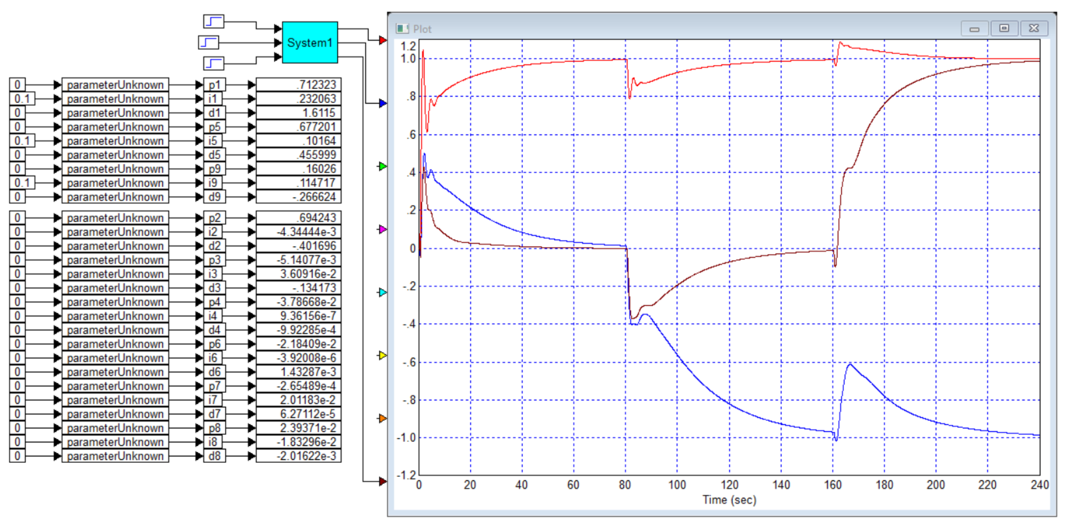
Figure 12.
Cost function for the case of example 5 according the project in Figure 11.
Figure 12.
Cost function for the case of example 5 according the project in Figure 11.
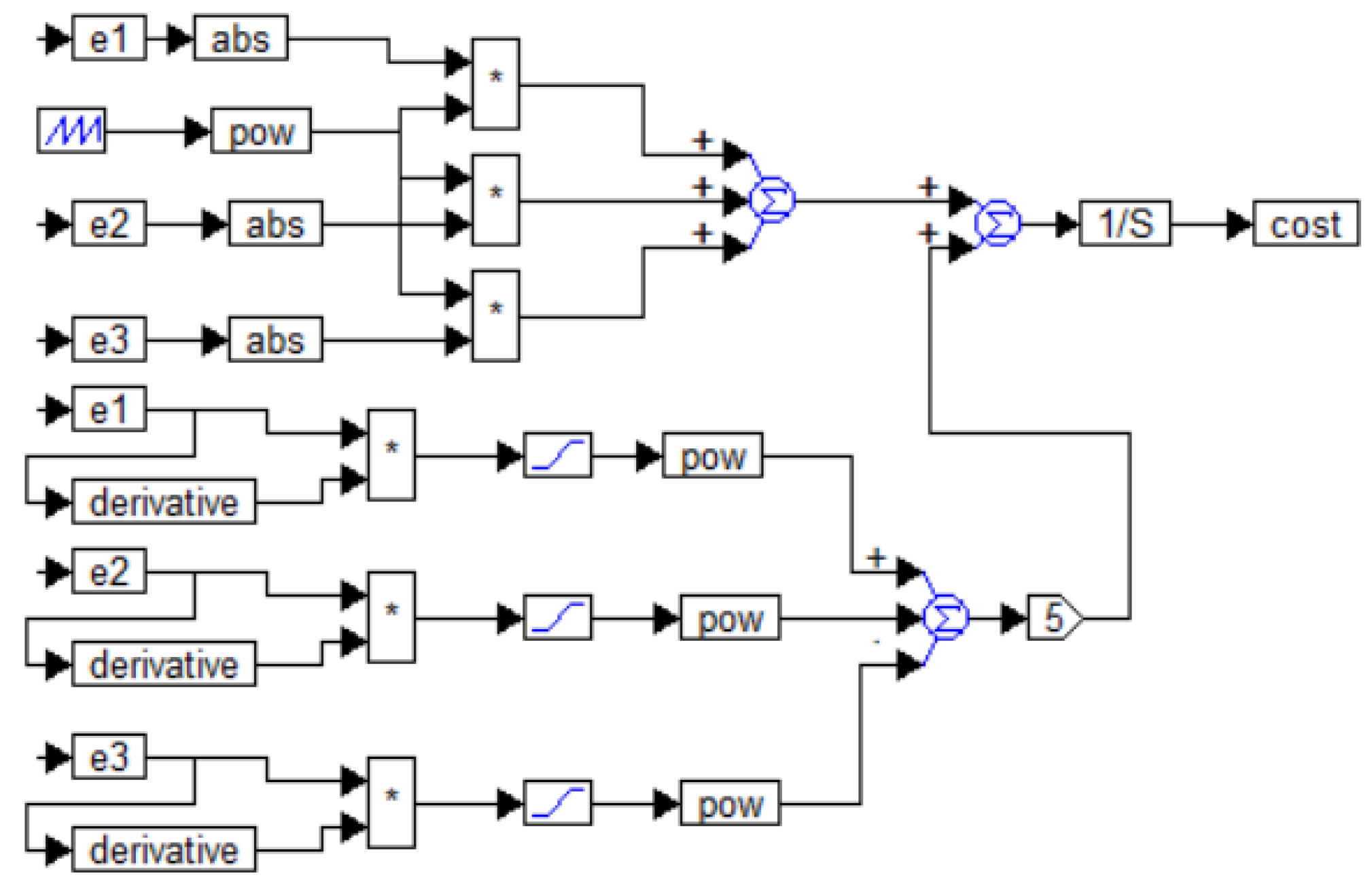
Figure 13.
Result when decreasing the weighting coefficient of the second member, fourth root.
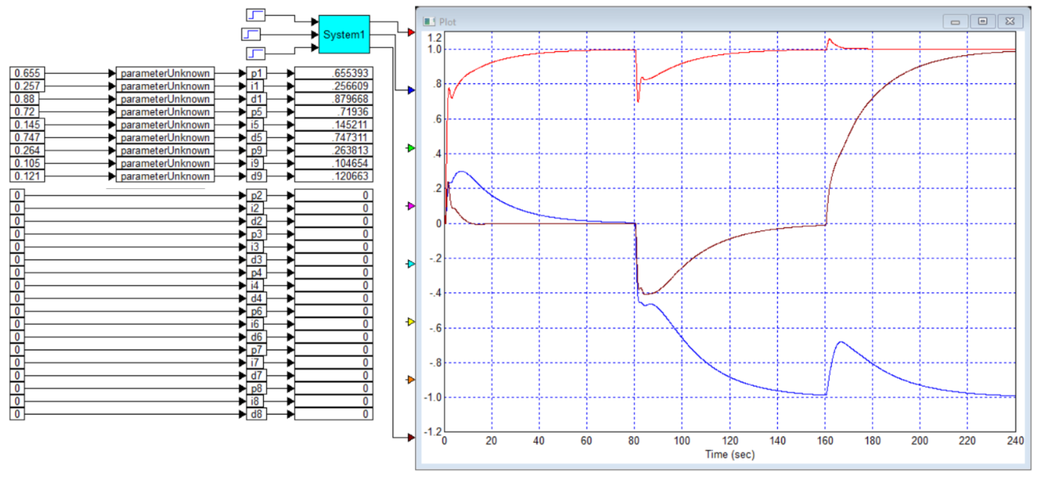
Figure 14.
Result when using a small weighting factor in the second term.
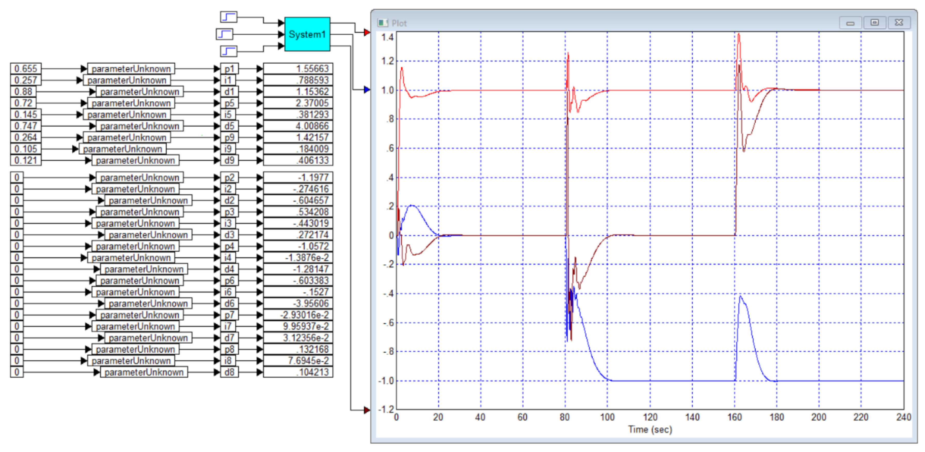
Figure 15.
Result when using the square root in the second term of objective function.
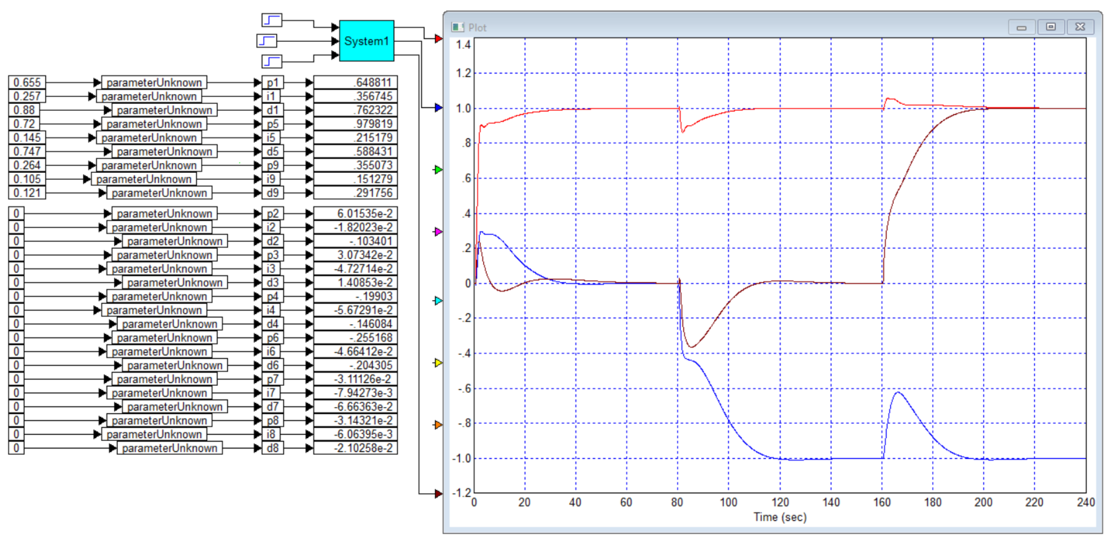
Figure 16.
Slightly worse result (more peaks in the first channel) when using the diagonal control.
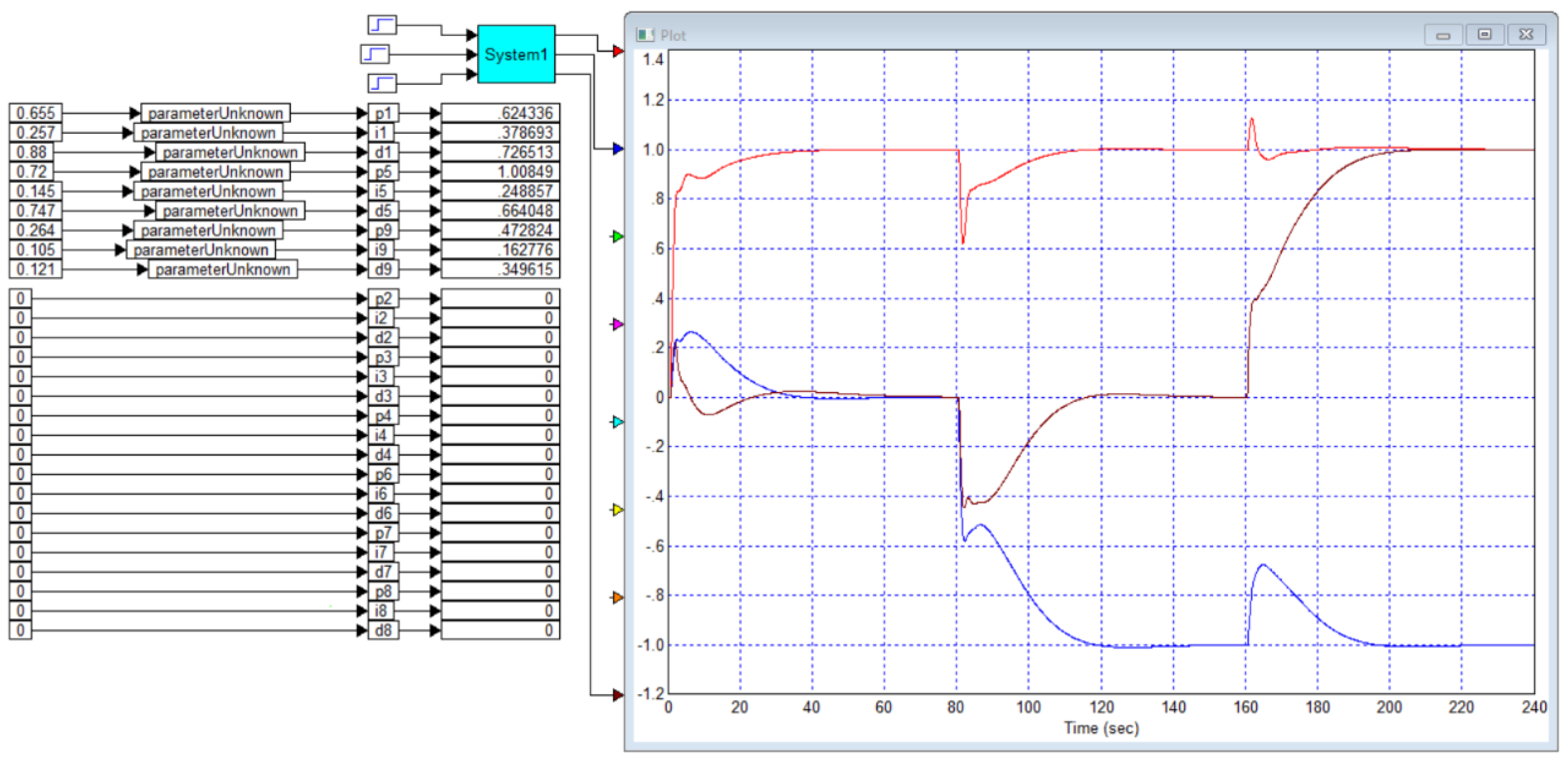
Figure 17.
The result of designing and optimizing the diagonal controller for example 6, the cost function is as in Figure 12.
Figure 17.
The result of designing and optimizing the diagonal controller for example 6, the cost function is as in Figure 12.
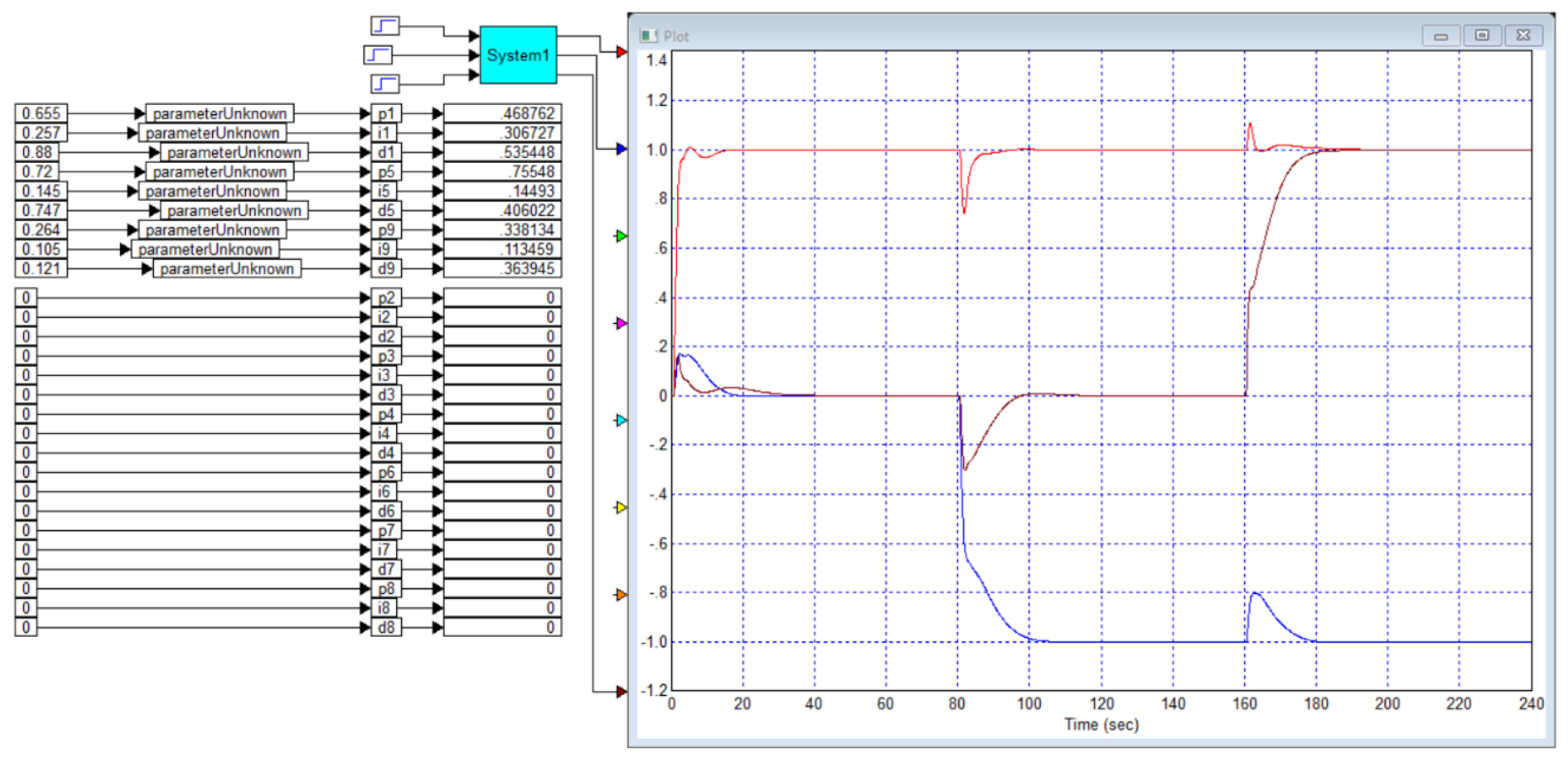
Figure 18.
Design and optimization result of the full controller for example 6, cost function as in Figure 12: the result is slightly better than in Figure 17: smaller responses in the first and in each channel when the task on the other channels goes.
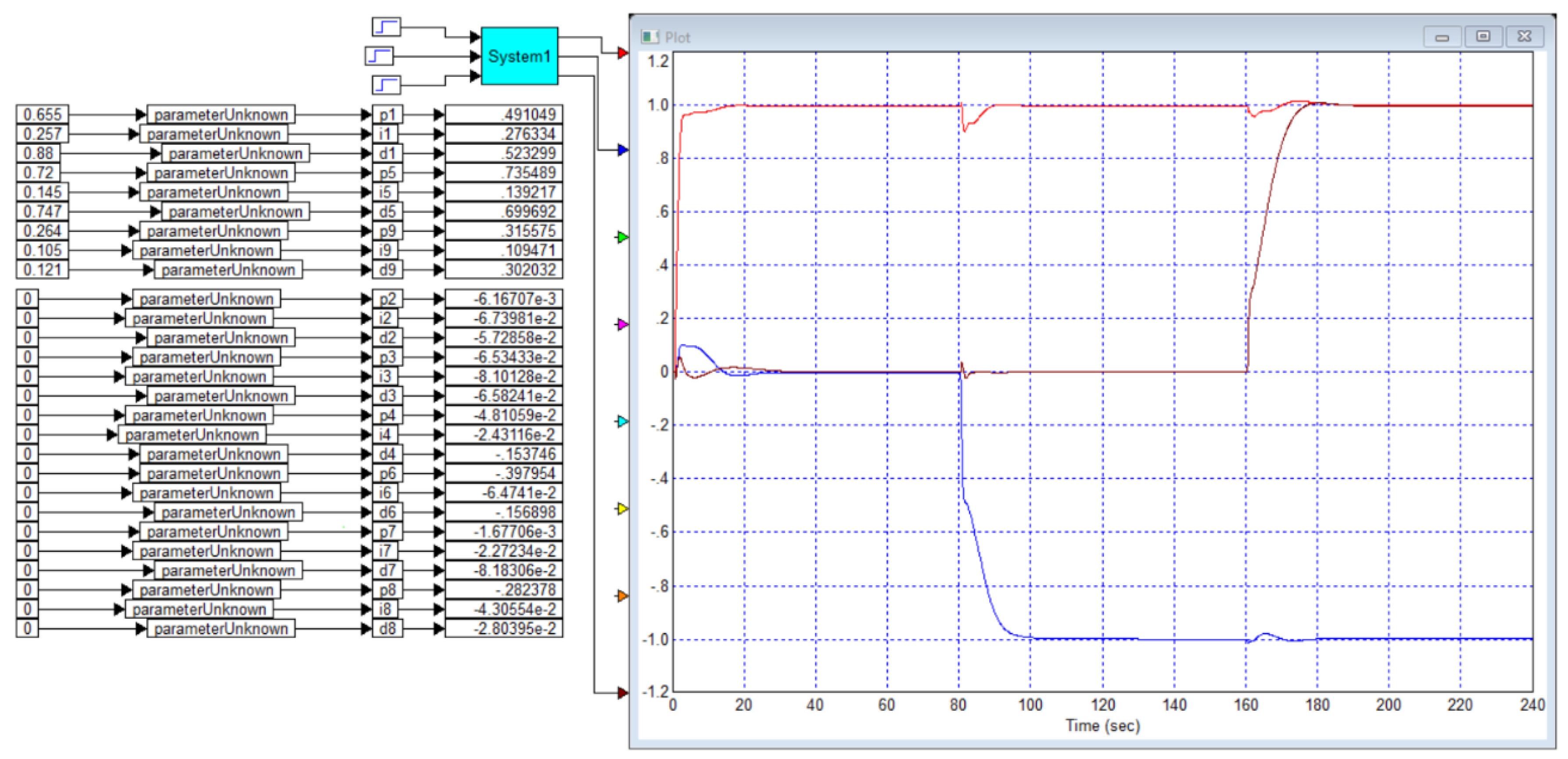
Figure 19.
Controller optimization project for the Example 7 object and the result for this case.
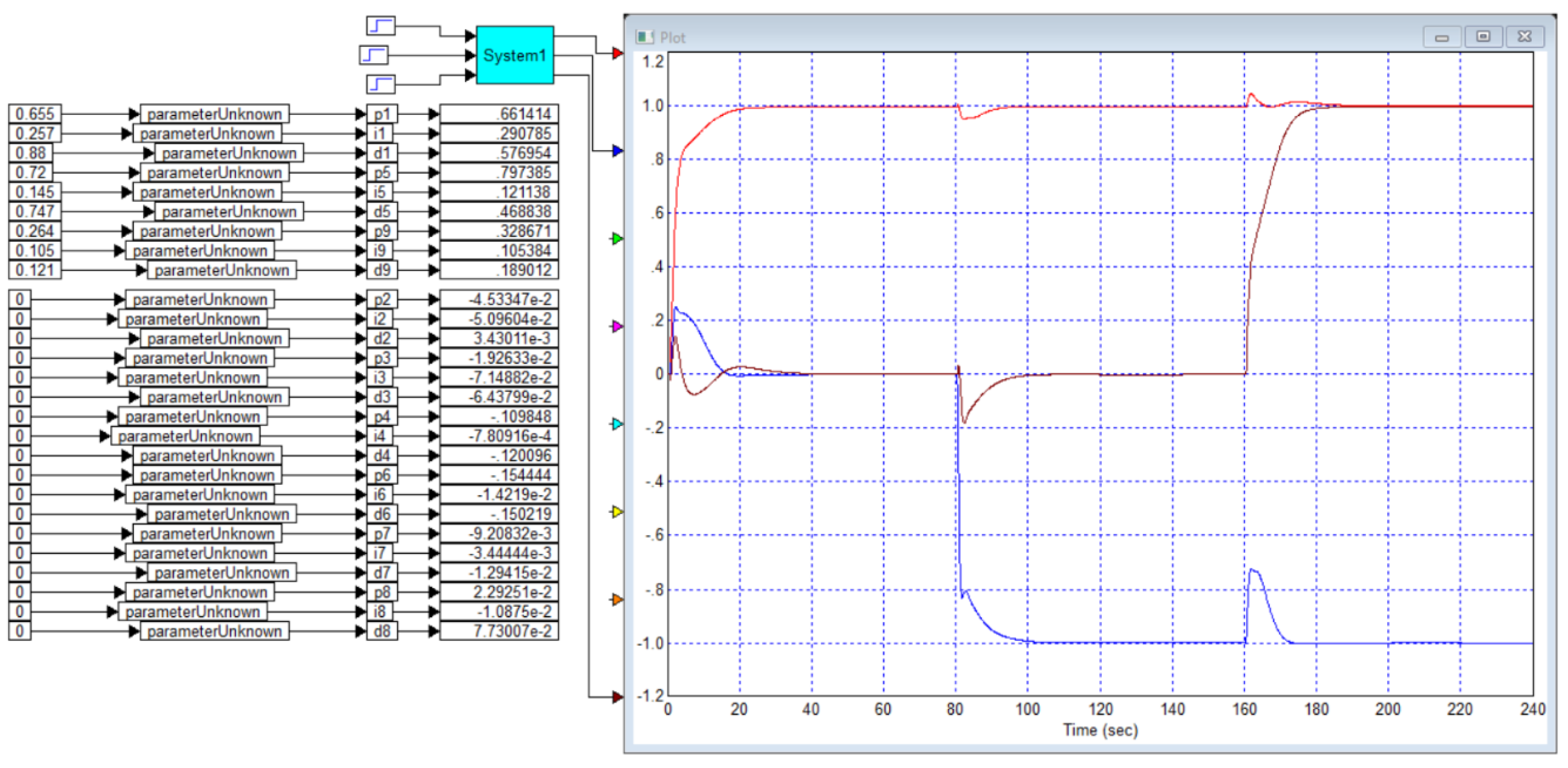
Figure 20.
Controller optimization project for the Example 7 object using individual weighting factors and the result for this case.
Figure 20.
Controller optimization project for the Example 7 object using individual weighting factors and the result for this case.
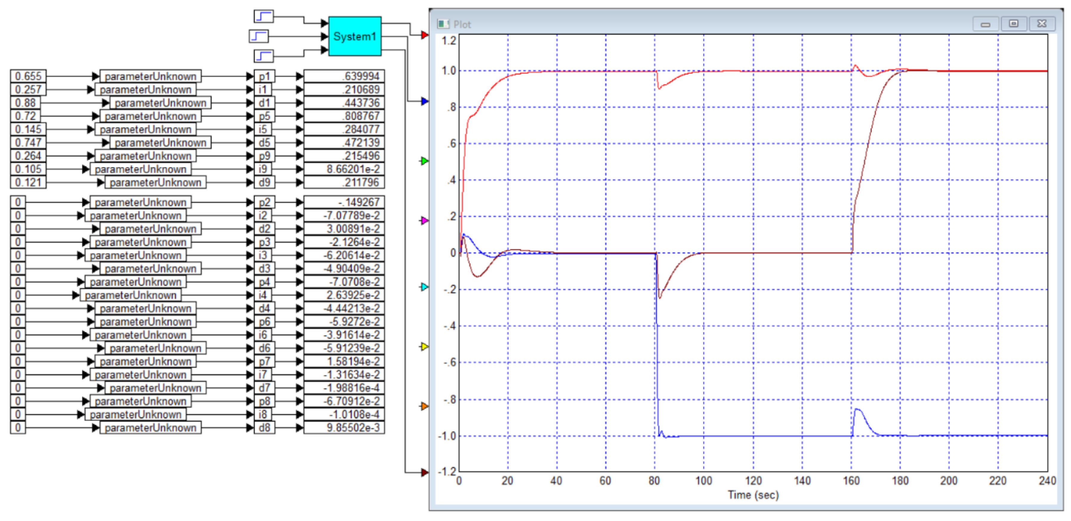
Figure 21.
Design and optimization result using three task transitions in each channel and the simplest cost function according to Example 8.
Figure 21.
Design and optimization result using three task transitions in each channel and the simplest cost function according to Example 8.
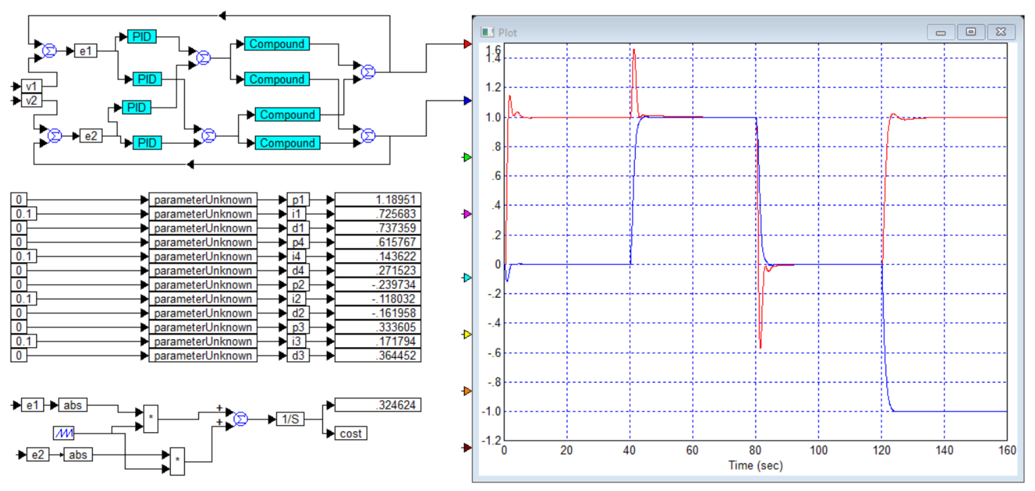
Figure 22.
Design and optimization result using one transition to the task in each channel and the simplest cost function according to Example 8.
Figure 22.
Design and optimization result using one transition to the task in each channel and the simplest cost function according to Example 8.
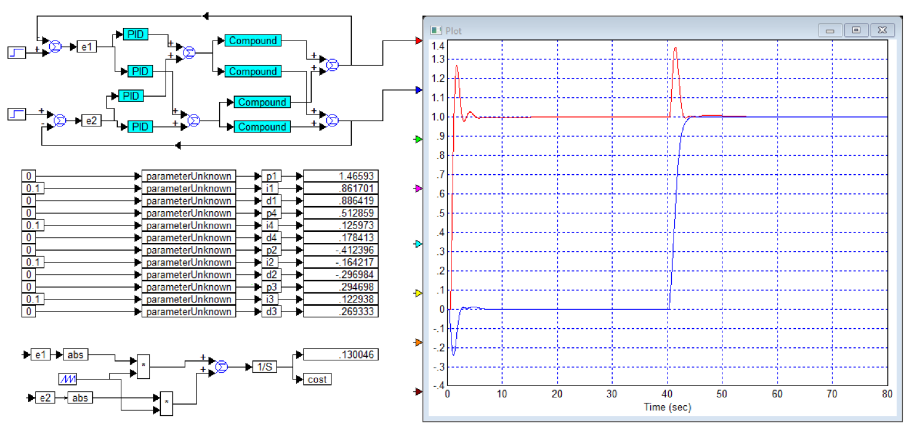
Figure 23.
Design and optimization result using four hops in each channel and a complex cost function that helps reduce overshoot.
Figure 23.
Design and optimization result using four hops in each channel and a complex cost function that helps reduce overshoot.
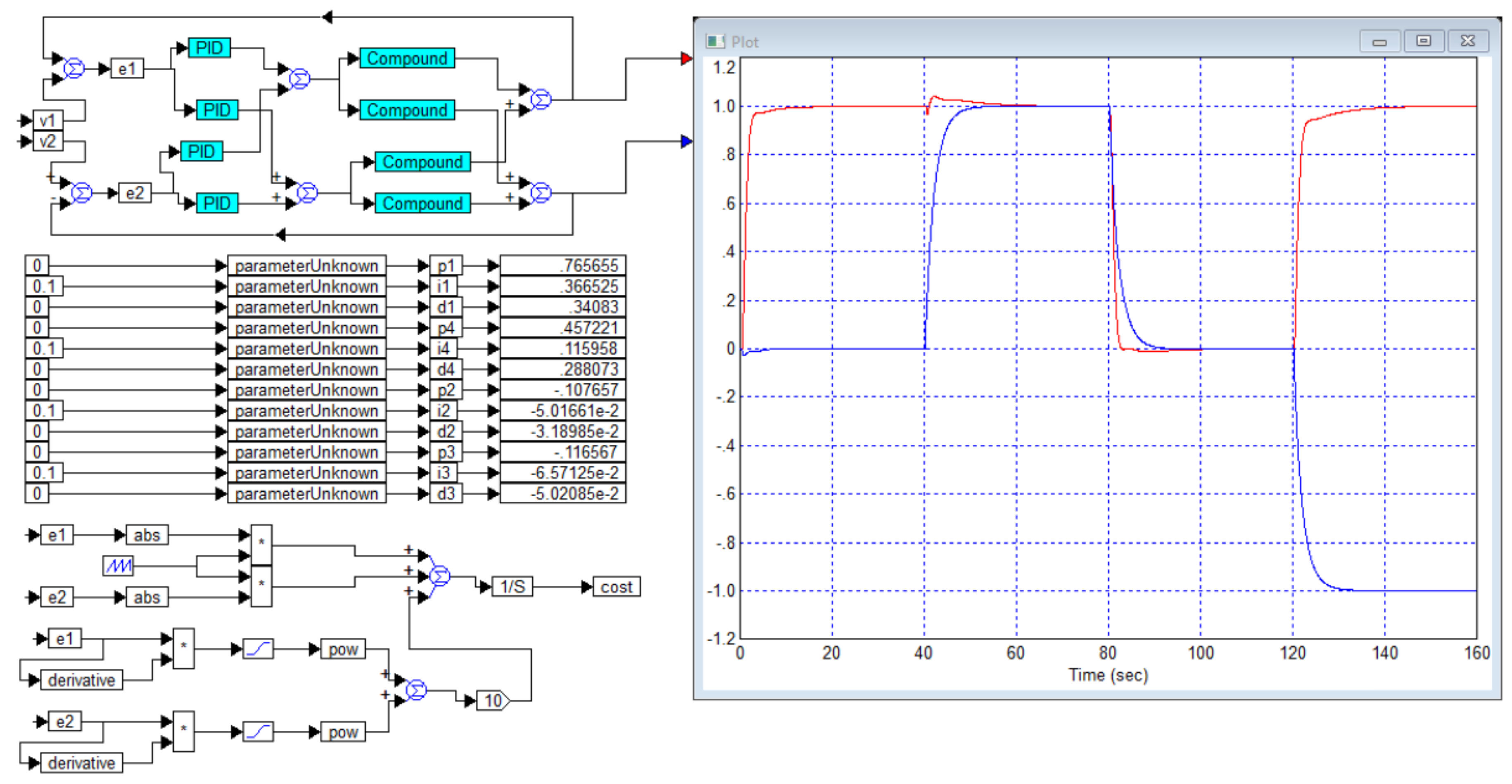
Figure 24.
System optimization project for the object from Example 9 (and from Example 2) using the test task from Example 8.
Figure 24.
System optimization project for the object from Example 9 (and from Example 2) using the test task from Example 8.
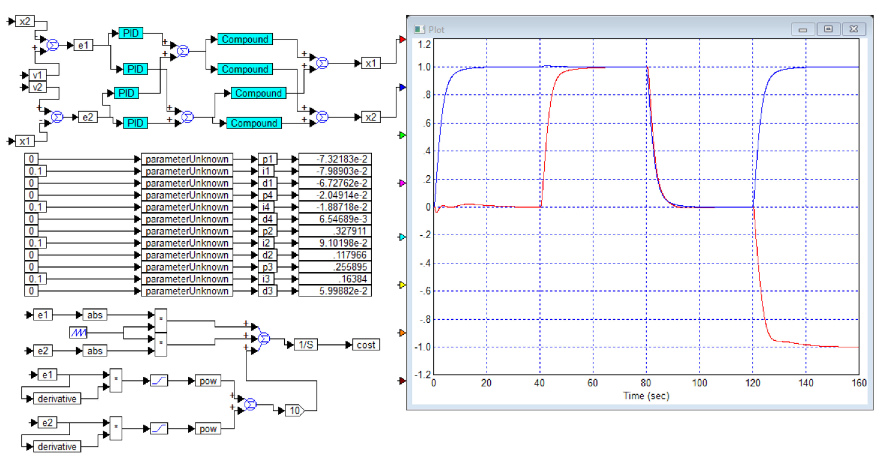
Figure A1.
Amplitude-frequency |W(ω)| and phase -frequency ϕ(ω) characteristics of a first-order object depending on the frequency on a logarithmic scale Lgω, according to the relation (A1).
Figure A1.
Amplitude-frequency |W(ω)| and phase -frequency ϕ(ω) characteristics of a first-order object depending on the frequency on a logarithmic scale Lgω, according to the relation (A1).
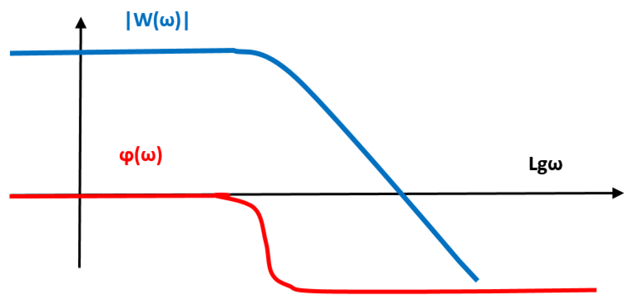
Figure A2.
Amplitude-frequency |W(ω)| and phase-frequency ϕ(ω) characteristics of a first-order object depending on the frequency on a logarithmic scale Lgω in the presence of a delay link, according to the relation (A2).
Figure A2.
Amplitude-frequency |W(ω)| and phase-frequency ϕ(ω) characteristics of a first-order object depending on the frequency on a logarithmic scale Lgω in the presence of a delay link, according to the relation (A2).
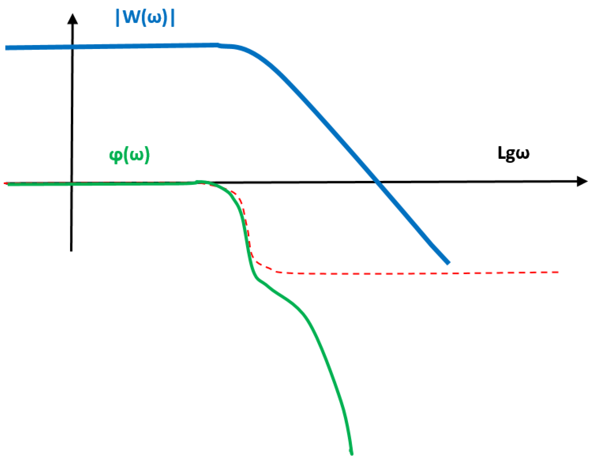
Figure 2.
Results of modeling the system according to example 1 from publication [29]: the red line shows the transient process obtained with the object and the PI controller proposed by the authors T i = 4, K p = 0.3679; the blue line shows the process obtained with the PI controller calculated by us using the numerical optimization method, with the controller coefficients: Kp = 0.4605, KD = 0.112 (which gives in terms of the coefficients of this publication Ti = Kp / KD = 4.1116).
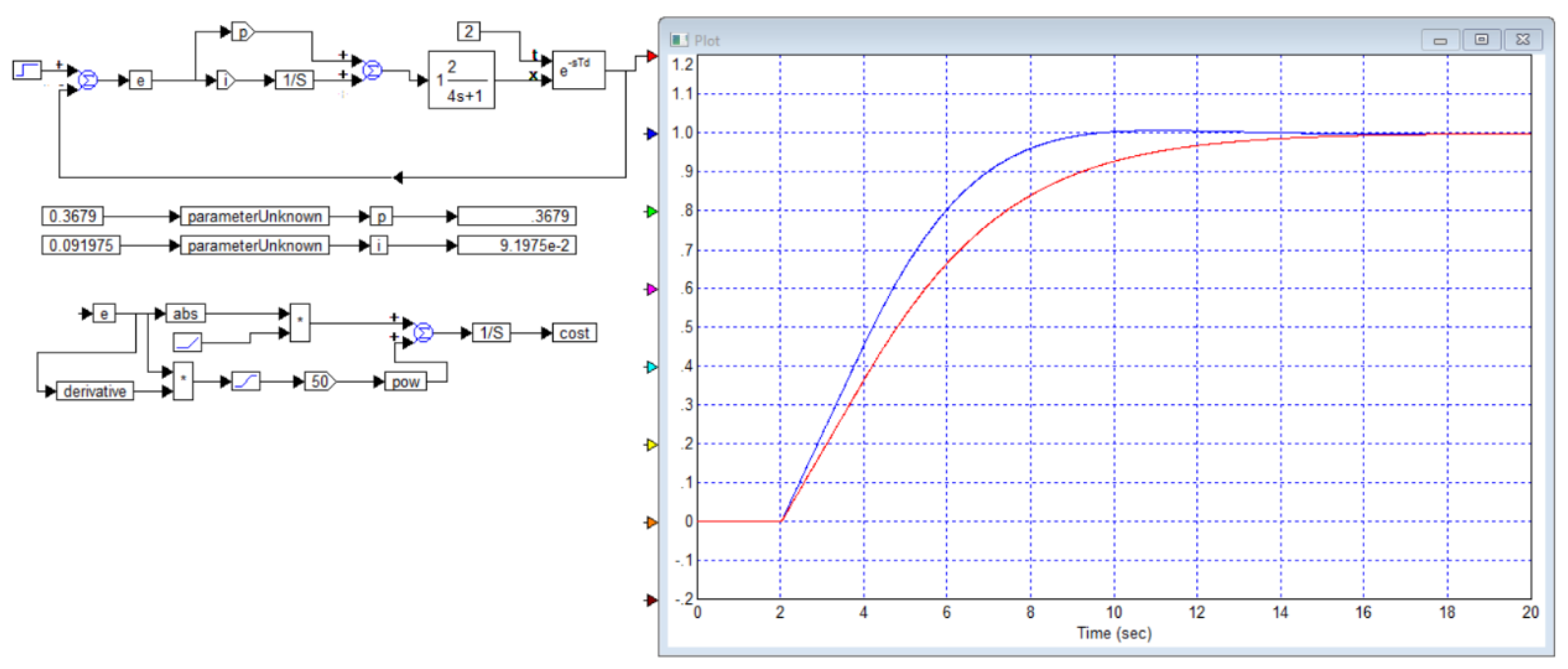
Figure 3.
Results of PI controller optimization for the system according to example 1 from publication [29]: Kp = 0.46112, KD = 0.1108, the duration of the transient process is 10 seconds, there is no overshoot.
Figure 3.
Results of PI controller optimization for the system according to example 1 from publication [29]: Kp = 0.46112, KD = 0.1108, the duration of the transient process is 10 seconds, there is no overshoot.
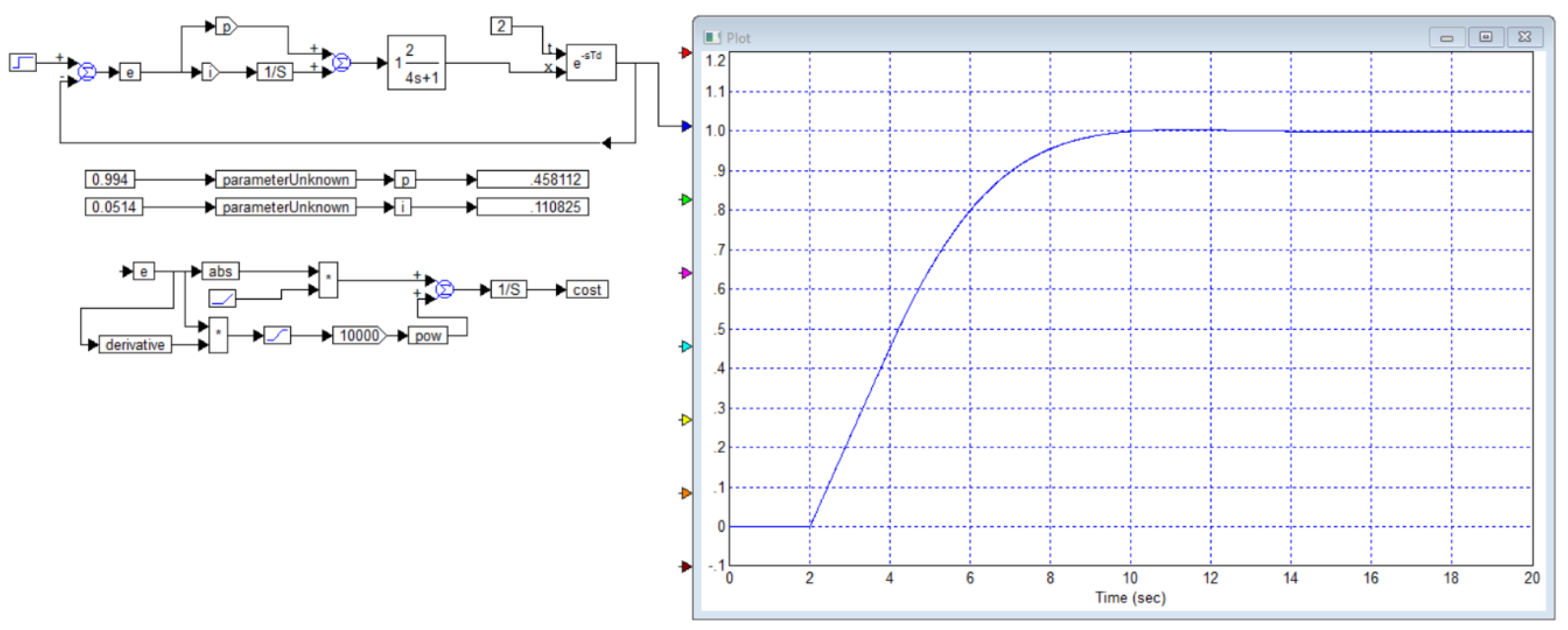
Figure 4.
Graph from publication [29] for a system consisting of an object with a transfer function of the form (B3) and a controller (B4).
Figure 4.
Graph from publication [29] for a system consisting of an object with a transfer function of the form (B3) and a controller (B4).
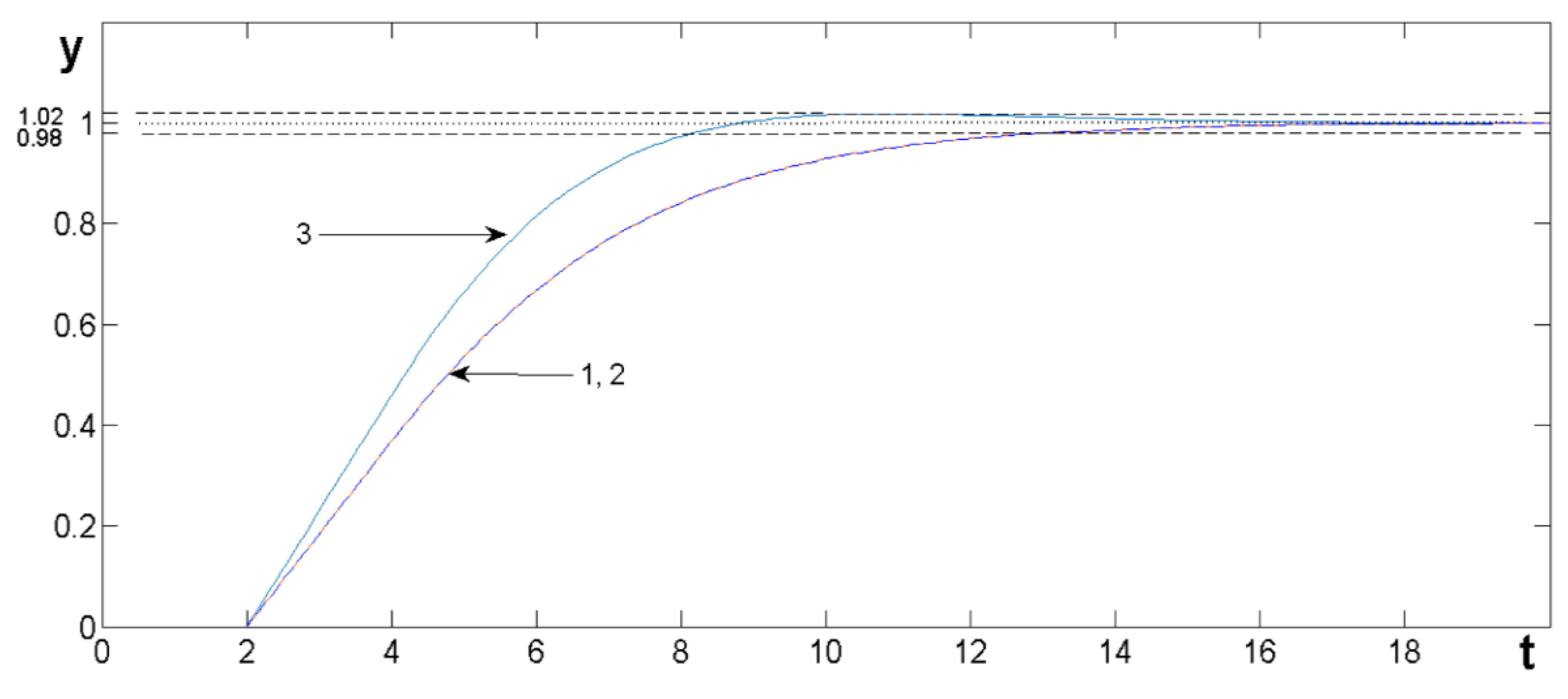
Figure 5.
Results of modeling the system according to example 2 from the publication [29]: the red line shows the transient process obtained with the object and the PI controller proposed by the authors; the blue line shows the process obtained with the PI controller calculated by us using the numerical optimization method, while the controller coefficients.
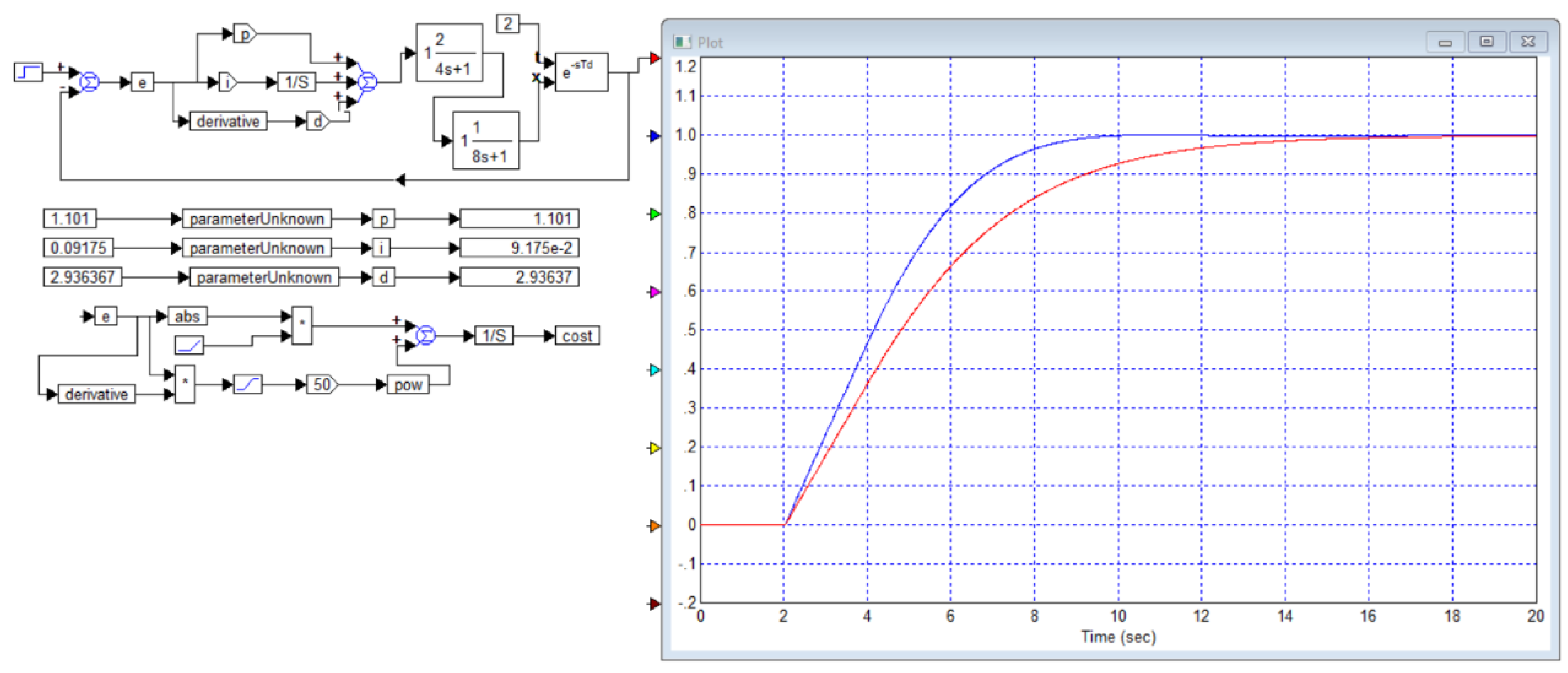
Figure 6.
Graph from publication [29] for a system consisting of an object with a transfer function of the form (B5) and a controller (B4) with a change in the time constant of the object model T = 4 sec; curve 1 is the original, curve 2 is an increase in the time constant by 20%, i.e. T = 4.8 sec, curve 3 is with a decrease in the time constant by 20%, i.e. T = 3.2 sec.
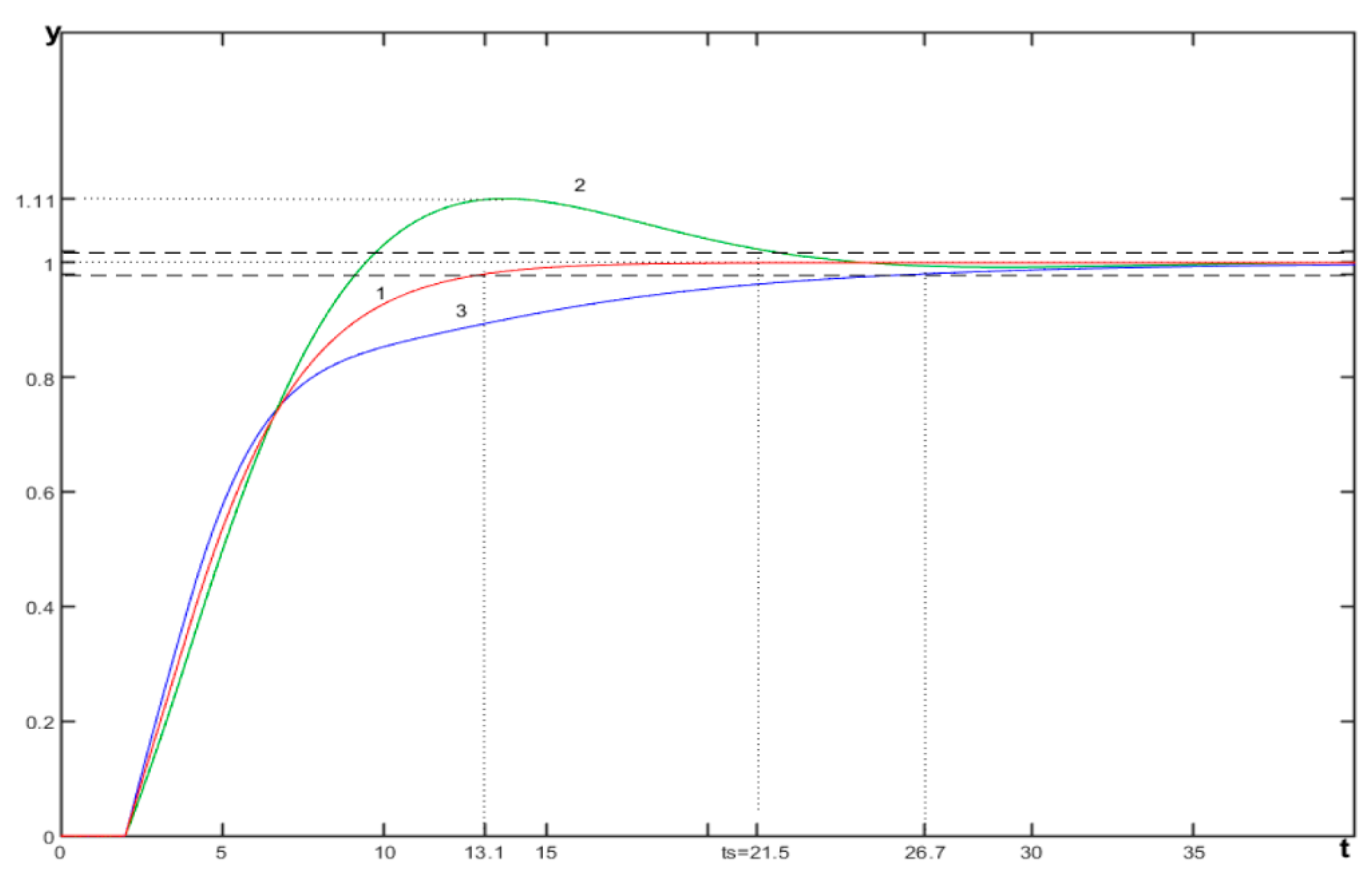
Figure 7.
Results of our modeling of the system from the publication [58] for an object with a transfer function of the form (B5) and a controller (B4) with a change in the time constant of the object model T = 4 sec; the blue curve is the original, the red curve is an increase in the time constant by 20%, i.e. T = 4.8 sec, the black curve is with a decrease in the time constant by 20%, i.e. T = 3.2 sec.
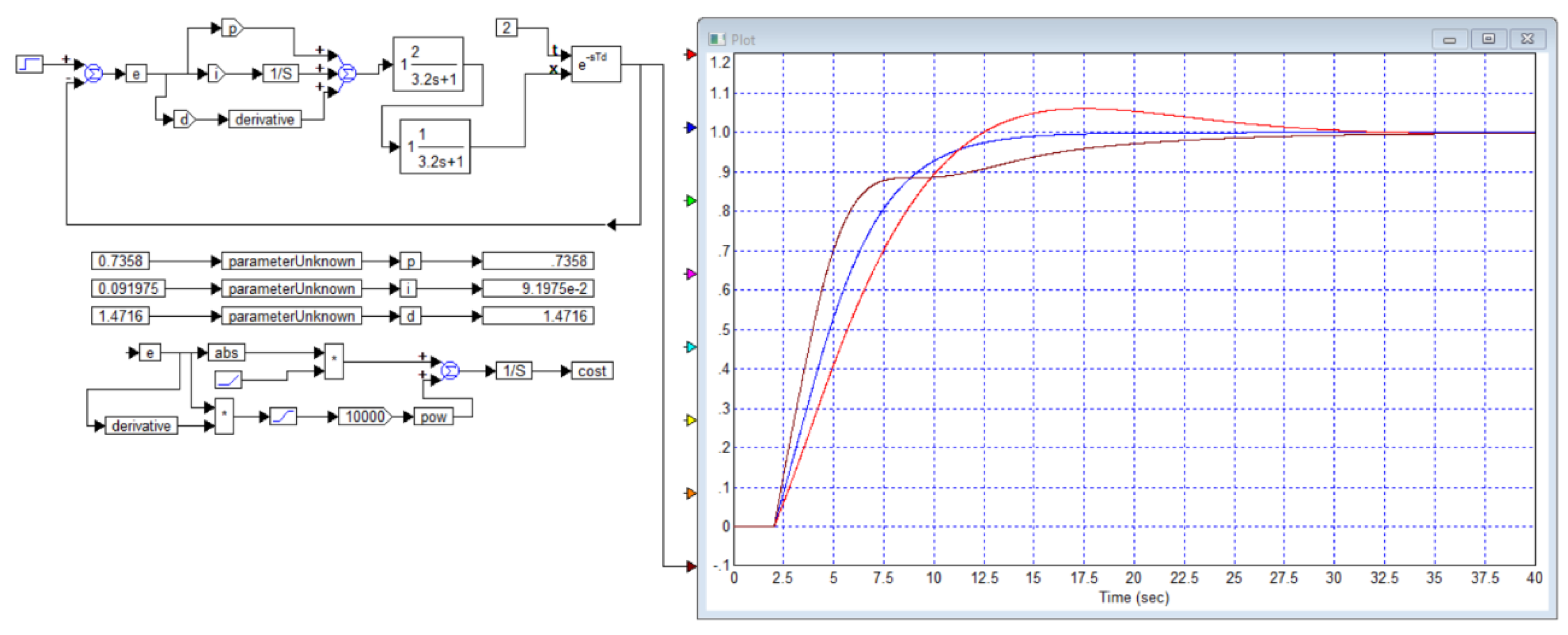
Figure 8.
The transient processes we calculated on the left for the simplified model (red line) and for the original model (blue line) for example 4 from publication [29], as well as the corresponding graphs from publication [58]: simplified model – line 1, exact model – line 2.
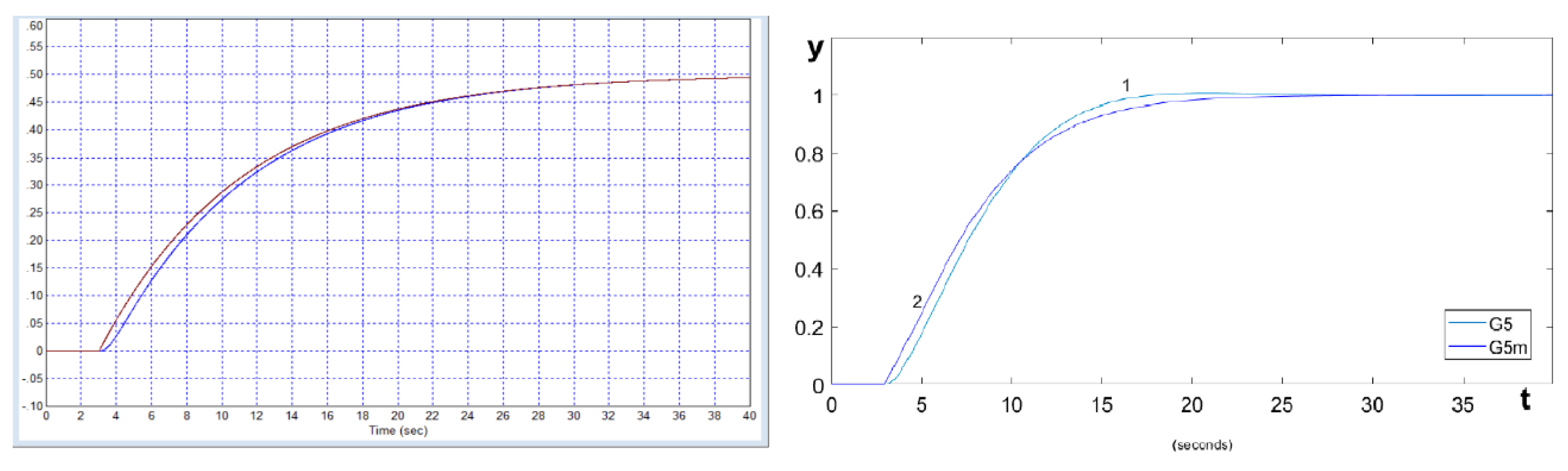
Figure 9.
Model of the system and transient processes in it according to Example 4 from the publication [29]: the blue line is the processes in the system calculated according to the exact mathematical model of the object, the red line is the processes in this system in the case where the regulator is calculated according to its approximation, which is proposed by the article [29].
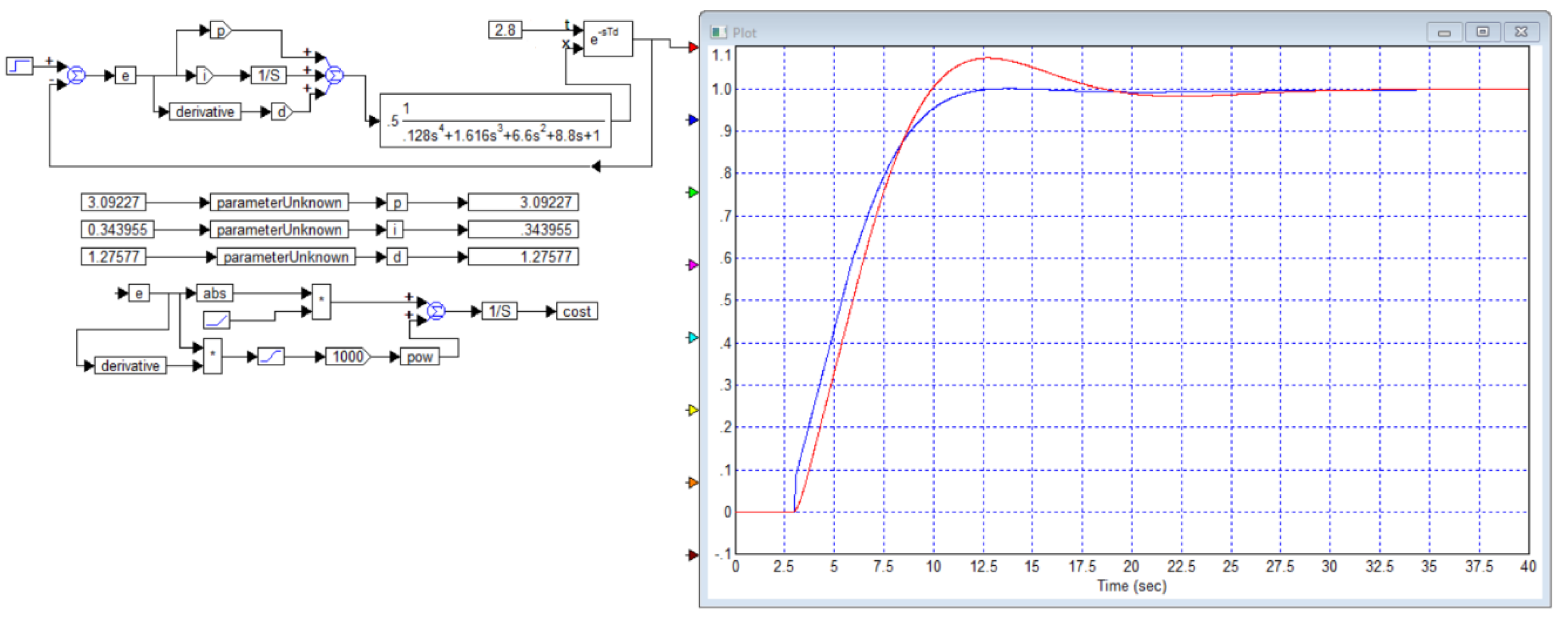
Figure 10.
Fragment with the problem statement for example 5 from the publication [29], which states that this example is taken from the publication [59].
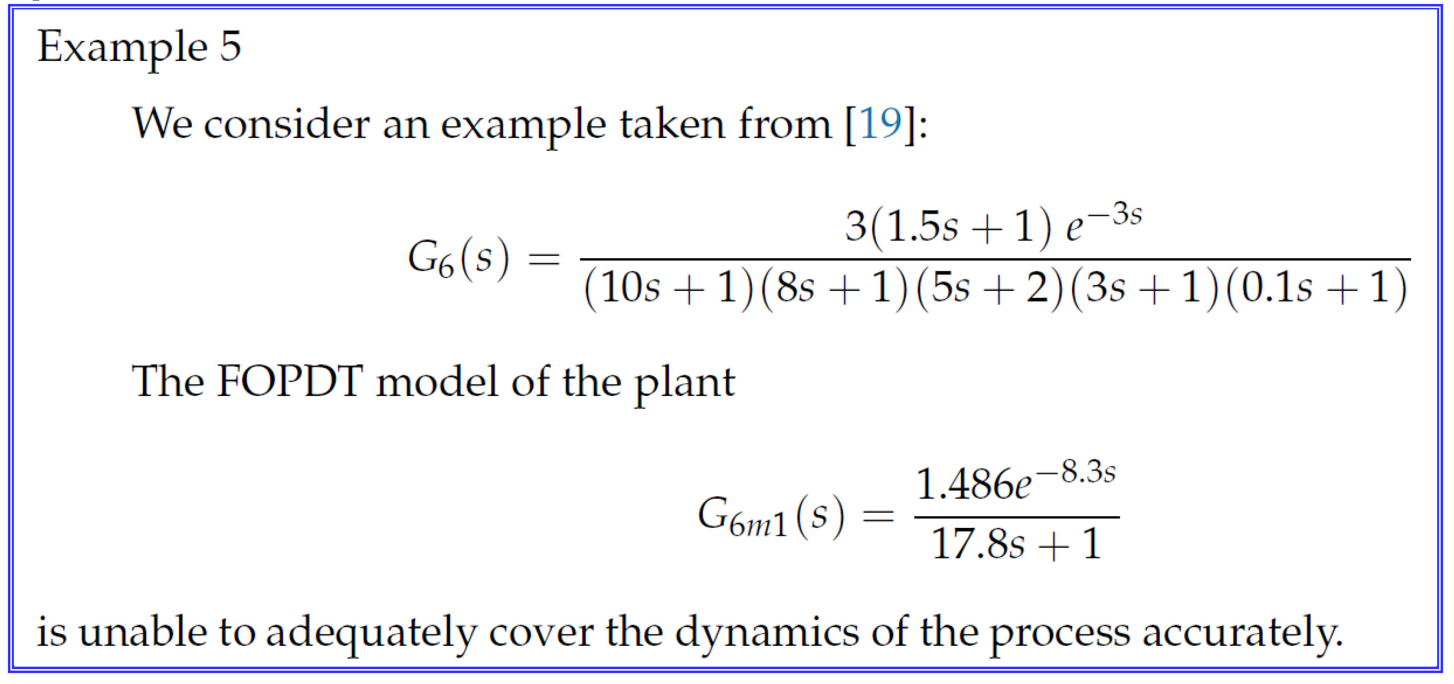
Figure 11.
The result of applying the controller calculated using a simplified model to control an object described by an exact model using the numerical optimization method for example 5 from publication [29] (red line), and for comparison, the process obtained in the system with this simplified model is shown by the blue line.
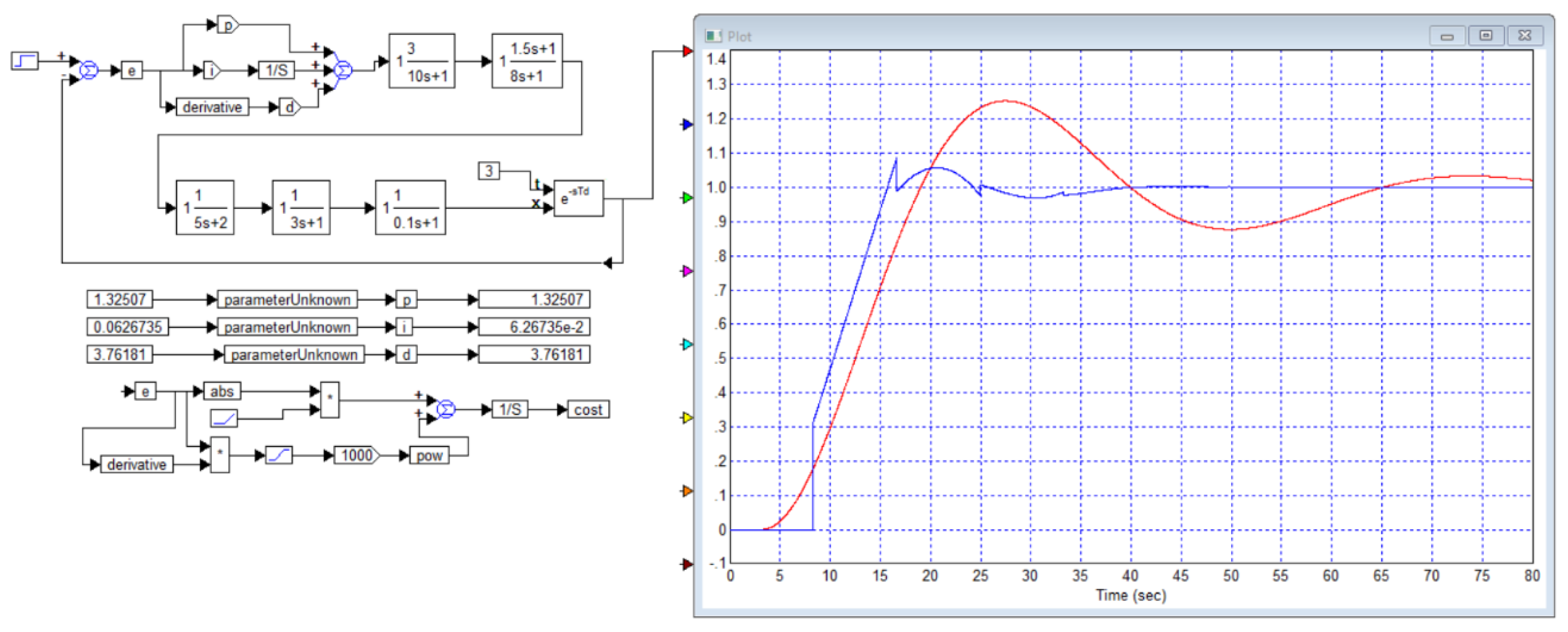
Figure 12.
The result of applying the controller calculated using the exact model to control this object from Example 5 in [29].
Figure 12.
The result of applying the controller calculated using the exact model to control this object from Example 5 in [29].
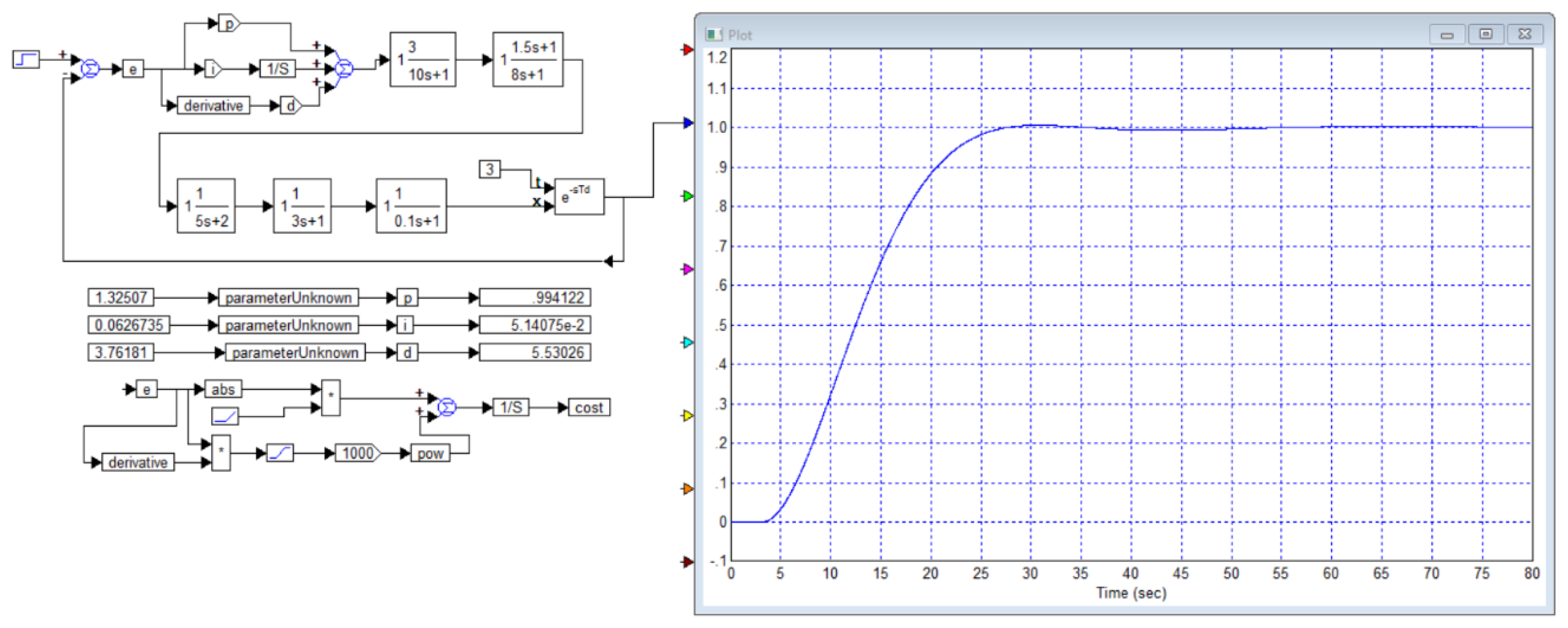
Figure 13.
Result of applying the controller proposed in publication [29] for example 5.
Figure 13.
Result of applying the controller proposed in publication [29] for example 5.
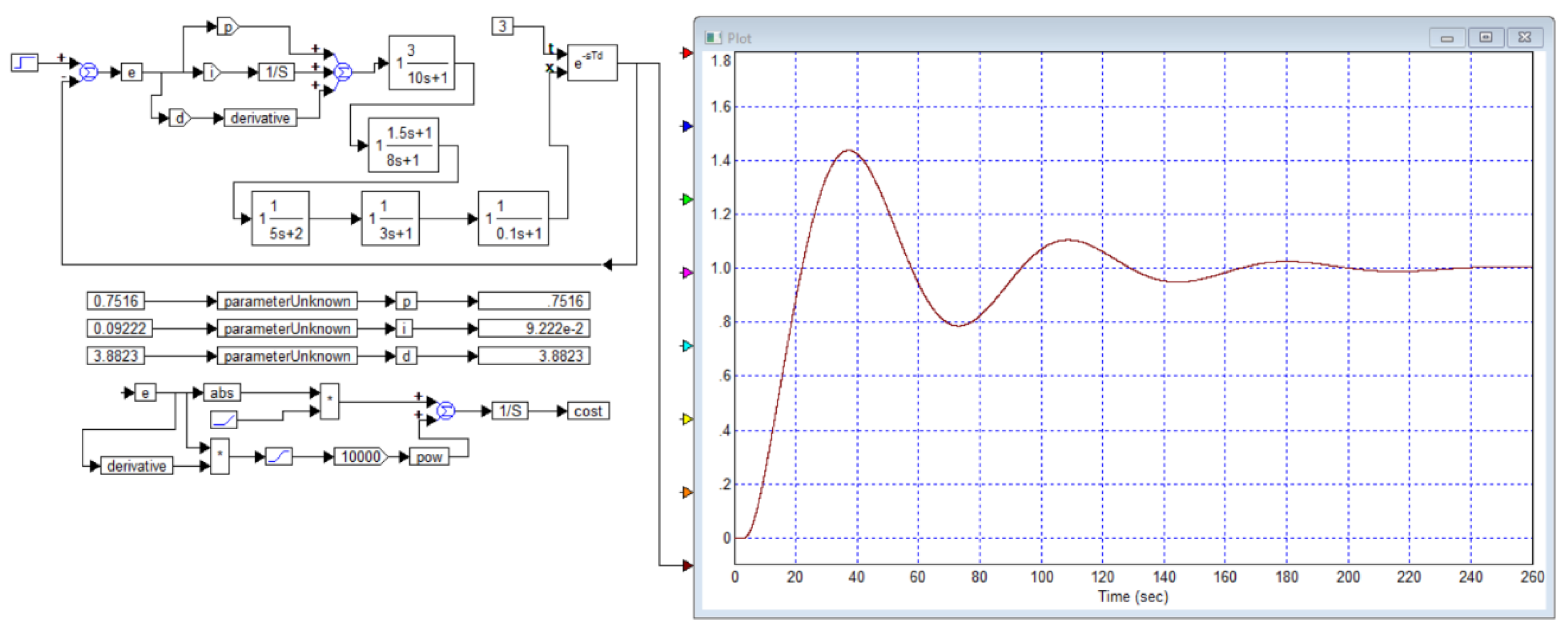
Figure 14.
Illustrative example from publication [60].
Figure 14.
Illustrative example from publication [60].
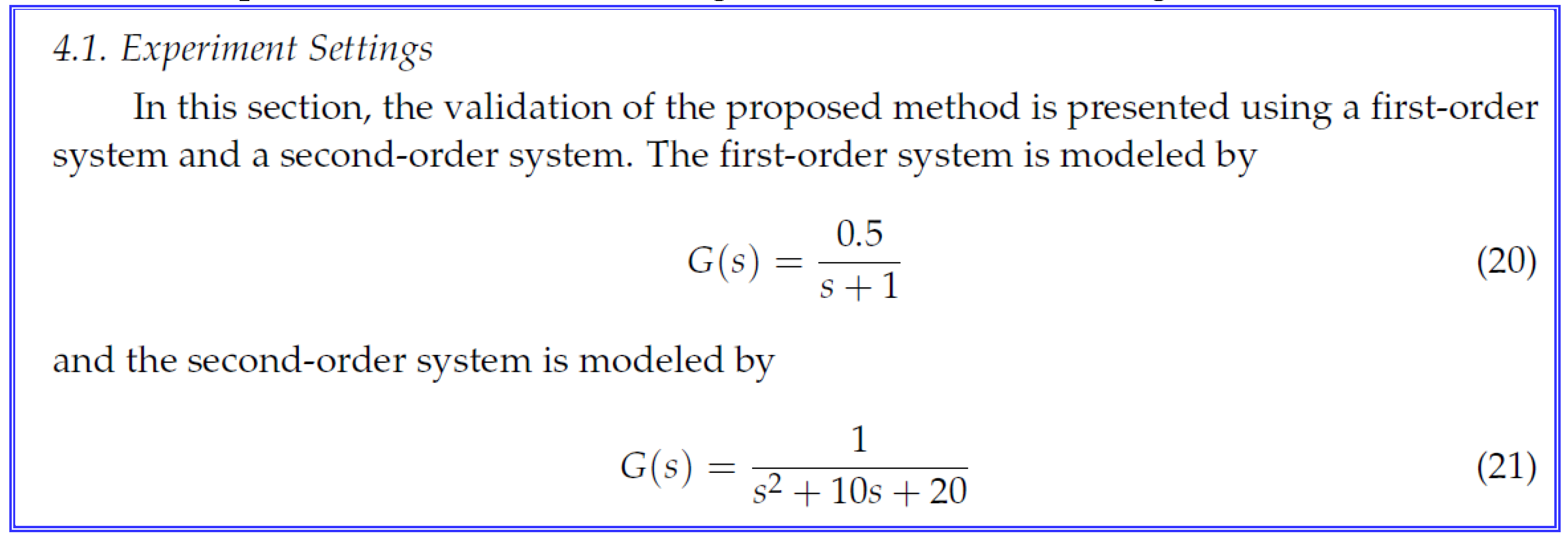
Figure 15.
Illustrative example from publication [61].
Figure 15.
Illustrative example from publication [61].
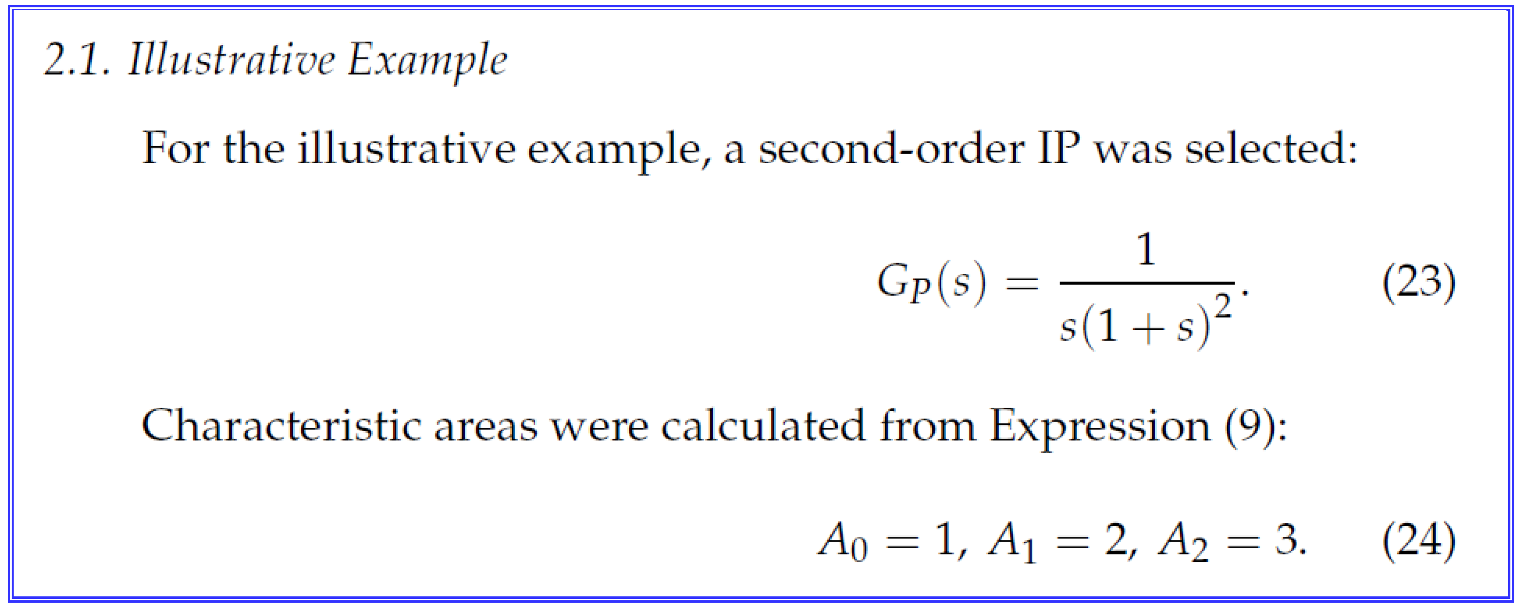
Figure 16.
Table of coefficients from publication [64], emphasis ours.
Figure 16.
Table of coefficients from publication [64], emphasis ours.
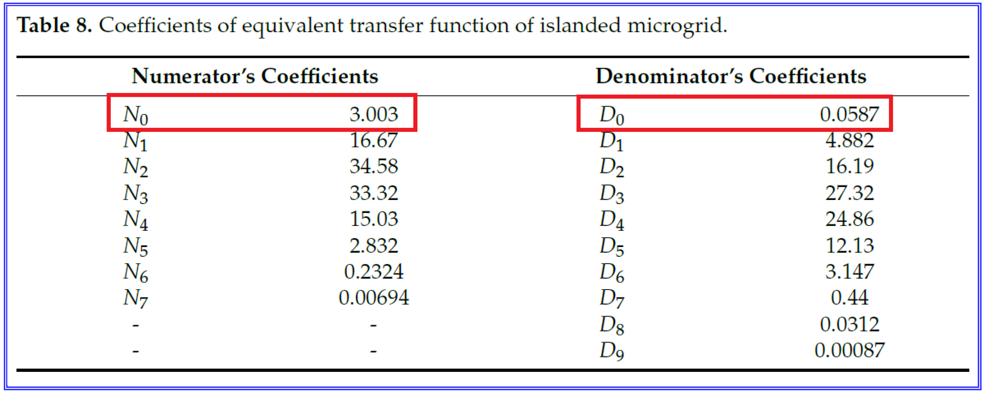
Figure 17.
Transient process graphs from publication [64], blue line – process at the output of the exact model, red line – process at the output of the approximating model.
Figure 17.
Transient process graphs from publication [64], blue line – process at the output of the exact model, red line – process at the output of the approximating model.
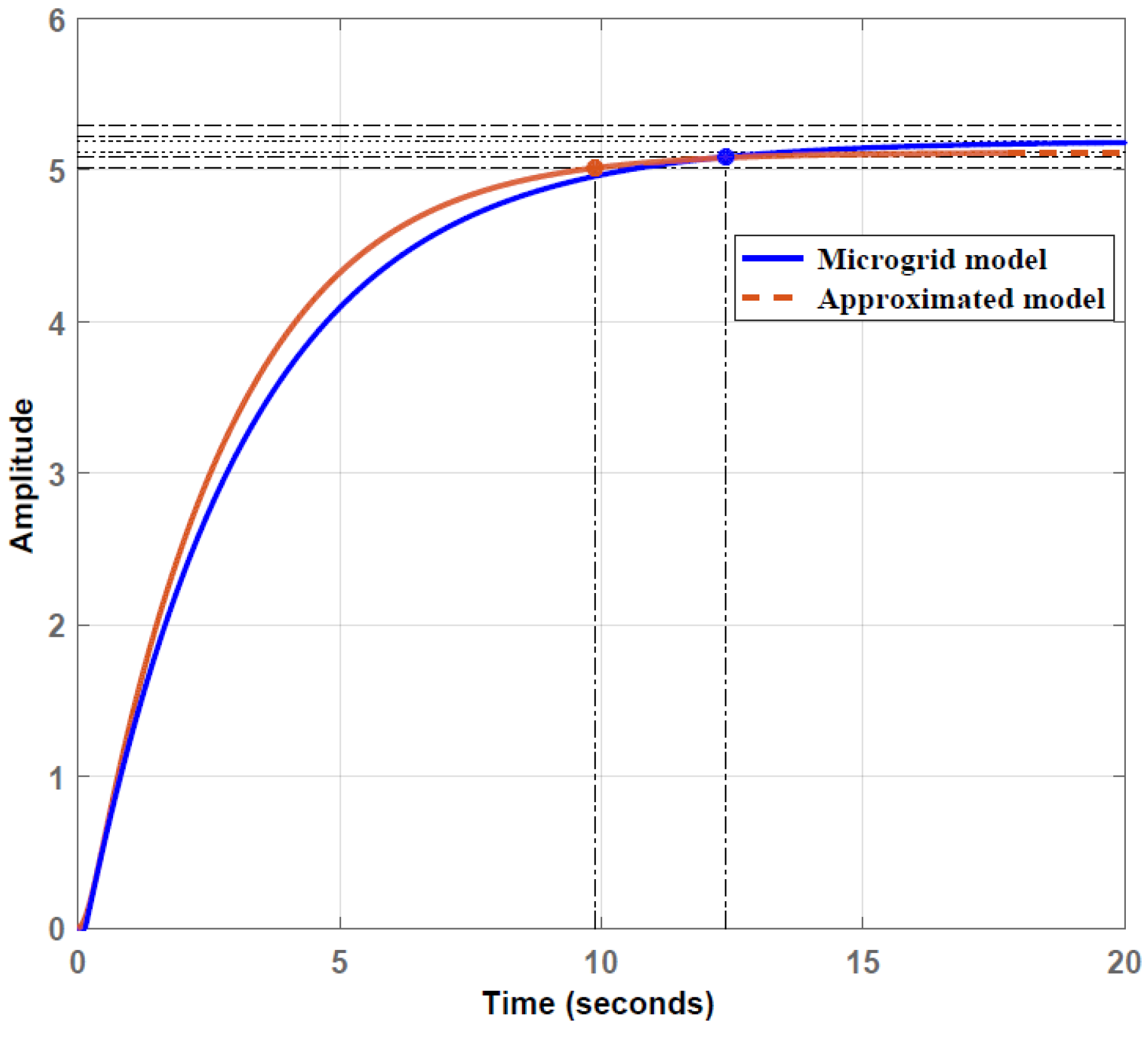
Disclaimer/Publisher’s Note: The statements, opinions and data contained in all publications are solely those of the individual author(s) and contributor(s) and not of MDPI and/or the editor(s). MDPI and/or the editor(s) disclaim responsibility for any injury to people or property resulting from any ideas, methods, instructions or products referred to in the content. |
© 2025 by the authors. Licensee MDPI, Basel, Switzerland. This article is an open access article distributed under the terms and conditions of the Creative Commons Attribution (CC BY) license (http://creativecommons.org/licenses/by/4.0/).
Copyright: This open access article is published under a Creative Commons CC BY 4.0 license, which permit the free download, distribution, and reuse, provided that the author and preprint are cited in any reuse.


