
Submitted:
28 November 2024
Posted:
29 November 2024
You are already at the latest version
Abstract
The reduction of noise and vibration is possible with passive, semi-active and active control strategies. If, especially self-adaptive control is required, it is necessary to evaluate the noise reduction potential before the control approach is applied to the real world problem. This evaluation can be based on a virtual model that contains all relevant sub-systems, transfer paths and coupling effects on the one hand. On the other hand the complexity of such a model has to be limited to focus on principal findings such as convergence speed, power consumption, and noise reduction potential. The present paper proposes a fully coupled electro-vibro-acoustic model for the evaluation of self-adaptive control strategies. The model consists of discrete electrical and mechanical networks that are applied to model the electro-acoustic behavior of noise and anti-noise sources. The acoustic field inside a duct, terminated by these electro-acoustic sources, is described by finite elements. The resulting multi-physical model is capable to describe all relevant coupling effects and enables an efficient evaluation of different control strategies such as local control of sound pressure or active control of acoustic absorption. It is designed as a benchmark model for the benefit of the scientific community.
Keywords:
Self-adaptive control
; Multi-physical simulation
; Electro-vibro-acoustic model
1. Introduction
The design of noise control strategies is impossible without basic knowledge on the theory of sound and vibration. The latter is described in many textbooks, for example in [1,2,3]. To design active noise control treatments, it is in addition also necessary to understand electro-mechanical coupling effects in order to describe actuators, filter-structures and sensors. These aspects of the theory of vibrations are for example described in [4,5]. If finally self-adaptive control strategies are taken into account, adaptive signal processing as described in [6,7,8,9] has to be studied in great detail. Especially the so-called Filtered-x Least Mean Square (FxLMS) algorithm [6,7,8] that is used to minimize the squared error signal detected at a well-chosen sensor position considering both a proper reference signal and the transfer behavior between actuator and sensor plays an important role in many applications as described in [5,7,8,9]. This algorithms is well understood and implemented in many applications. It is used for decades also considering variations of the original implementation [10].
For many applications it has been sufficient to concentrate on Linear Time-Invariant (LTI) systems. An actual survey on the application of Active Noise Control (ANC) considering linear system behaviour has been presented in [11]. However, in many situations it is also necessary to cover non-linear effects. An actual survey on the application of ANC to non-linear system is to be found in [12]. Recently, a novel approach using a so-called Brain Storm Optimization (BSO) algorithm for active control of non-linear systems has been proposed in [13].
Considering the above named referenced that represent only a non-complete selection of all publications in this filed one can conclude that the concept of self-adaptive ANC as well as its application to LTI systems is well understood. Thus, its application should be in the spot light of ongoing research. One can also conclude that nowadays research is also focussed on non-linear effects. For this reason it is obvious to ask: Is it necessary to write another paper focussing on linear systems? From the point of view of the author the answer is yes. This is especially true, if the aspect of benchmarking is taken into account.
It is of course possible to study a wide range of publications reporting on the design as well as on the performance evaluation of ANC. This is especially true for active control of plane waves in one-dimensional wave guides [14,15,16]. However, a drawback of many publications is that the electro-mechanical parameters describing the electro-mechanical parts are not documented in such a way that a reproduction of the relevant findings is supported without limitations. In contrast to the above named references also sophisticated mathematical models have been presented to describe the multi-physical problem of ANC based on detailed description of the model parameter, compare [17]. Unfortunately self-adaptive control has not been taken into account in this particular reference.
Summarizing these findings a simple Electro-Vibro-Acoustic (EVA) model that can be used to benchmark self-adaptive ANC approaches is (from the viewpoint of the author) still missing in the scientific community. For this reason the present paper proposes such a simple EVA model that is based on a limited number of Degrees Of Freedom (DOF). The latter are introduced to describe the propagation of sound in a one-dimensional wave guide without non-linear effects. This model is presented in combination with a detailed description of the physical parameter of the electro-mechanical components as well as of the acoustic wave guide. It consists of discrete electrical and mechanical networks that are applied to model the electro-acoustic behavior of noise and anti-noise sources. The acoustic field inside a duct, terminated by the electro-acoustic sources, is modelled using the Finite Element Method (FEM). The resulting EVA model is capable to describe all relevant coupling effects and enables an efficient evaluation of self-adaptive control strategies such as local control of sound pressure or active control of acoustic absorption. It is designed as a benchmark model for the benefit of the scientific community.
The paper is structured as follows. Multi-physical modelling and self-adaptive control strategies based on the FxLMS algorithm are described in section 2. This section also includes comments on numerical integration. The behaviour of the passive system (without active control) is analysed in section 3, whereas the noise control potential of two control strategies is discussed in section 4. The paper closes with section 5 presenting a short summary of the main findings.
2. Multi-Physical Modelling and Self-Adaptive Control Strategies
In order to study self-adaptive control of sound, a multi-physical approach to an EVA system is proposed in the upcoming section. LTI system behavior is assumed for all subsystems. The latter are given by electro-dynamical loudspeaker and an acoustic duct. This subsystem represents the one-dimensional acoustic wave guide. At first the fully-coupled EVA model is introduced. Afterwards some comments will be given on the numerical solution of this model. In a second step two self-adaptive control strategies based on the FxLMS algorithm will be outlined.
2.1. A fully Coupled Electro-Vibro-Acoustical Model
As described in section 1 the proposed benchmark model is given by an acoustic duct of length and cross section terminated by the primary noise source at position x = 0 and the secondary source (anti-noise source). The latter terminates the duct at the position x = L. For further investigations five “sensor-positions” have been considered. The position of the primary source is identical to the position , and the position of the secondary source is identical to the position .
The equations of motion of these electro-mechanical networks are based on the electric charge , the displacement of the loudspeaker membrane , and the sound pressure defined at the positions . The associated ordinary differential equations (ODE’s) are given by
where is the inductance of the electrical network at position , is the electric resistance, is the capacity and is the electromagnetic force factor. is mass of the loudspeaker membrane at position , is its viscosity, and is the mechanical stiffness of the membrane. The external excitation is given by the voltage with applied at the primary and secondary loudspeaker.
As proposed in [5] the acoustic field inside the duct is modelled by finite elements, considering the speed of sound and the density as the relevant material properties. In the present approach four finite elements of length with linear shape functions have been used to establish a simple discrete model. The latter is given by
where are the sound pressure data determined at the positions . Acoustic sources inside the duct have not been taken into account. For this reason the right hand side of (2) is zero in every row.
The EVA model proposed in this paper contains nine DOF’s summarized in the (9x1) column matrix such as
The right hand side is also represented by a (9x1) column matrix that contains the external excitation prescribed at the loudspeaker such as
The fully coupled EVA model can be established in matrix notation such as
where is the (9x9) generalized mass matrix, is the (9x9) generalized damping matrix, and is the (9x9) generalized stiffness matrix. It should be noticed that all these matrices are non-symmetric. Thus the proposed model can also be used as a benchmark in a bi-modal decoupling approach as described in [18]. Using the abbreviations
the elements of these matrices can be presented such as
2.2. Comments on Numerical Integration, Frequency Domain Analysis and Generalized Eigenvalues
Considering only time-harmonic excitation signals, the EVA model defined by (5) – (9) can be solved analytically in time-domain. However, if also more sophisticated excitation signals have to be taken into account, a numerical solution is more convenient. Following the implementation of the original Newmark algorithm [19] that is proposed in [20] it is possible to analyze a broad range of excitation signals using a simple and robust algorithm for the numerical solution of second-order ODE’s. This integration schema can be summarized as follows. The new values of the dependent variables at the discrete time step are obtained from the dependent variables at the previous time as well as from their first and second time derivative such as
where is the sample time. The new value for the second time derivative is calculated such as
where represents the right hand side of (9) at the discrete time step . The new value of the first time derivative can subsequently be determined such as
Initial values must be defined for all these quantities such as
For time-harmonic excitation the solution of the EVA model described by (5) – (9) can be written in matrix notation such as
where is the imaginary unit and is the angular frequency that is associated to the excitation frequency . The (9x9) complex compliance matrix contains all Frequency Response Functions (FRF’s) of the system.
To study operational mode shapes at a given frequency it is possible to use the so called Transmissibility Functions (TMF’s). In order to define these quantities it is necessary to define one FRF as reference. If the response at position 1 due to excitation at position 1 is used as reference, it is possible to define eight non-trivial TMF’s out of the first column of such as.
where contains the deviation in both magnitude and phase between the response at position compared to the chosen reference position at the specific angular frequency Please notice that in contrast to a FRF a TMF can only be interpreted frequency by frequency because it describes an operational mode shape and not the response characteristic of a dynamic system.
In order to verify the results of numerical simulations it can be useful to determine the eigenvalues of the EVA model. Based on the state variables
It is possible to define a first order system of ODE’s on the state variables such as
where the (18x18) matrices and are given by
If the (18x1) column matrix is described by the associated complex eigenvalues can be derived from the generalized Eigenvalue Problem (EVP),
The imaginary part of these eigenvalues can be used to verify the resonance frequencies hat can be determined in time-harmonic analysis and numerical simulations.
2.3. Comments on Adaptive Algorithms
The self-adaptive control strategies applied in this investigation are based on the LMS algorithm. The latter has been originally proposed in [21]. However, in order to include the effect of the so called secondary path, the power normalized FxLMS algorithm, compare [6,7,8,9,10] considering one reference signal has been used.
In an approach to active control of sound this algorithm can be applied to adapt FIR filter (each of length ) in order to drive control sources. The signals generated by these anti-noise sources are passed though secondary paths in order to minimize the instantaneous squared error determined at sensor positions.
An algorithmic summary of the FxLMS algorithm is given in (19), where is the l-th power normalized step size and is its non-normalized counterpart. In order to prevent a division by zero it is also necessary to introduce a minimum value of the signal energy. The latter is represented by .
If self-adaptive control can be limited to one reference signal as well as to one controller driving only one secondary source in order to reduce one error signal at one sensor position (19) reduced to the version or single-channel version of the FxLMS algorithm that is easy to implement. In such a situation it is only necessary to identify one secondary path .
A compact summary on single-channel self-adaptive filtering based on the power normalized LMS algorithm applied to system identification has recently been presented by the author [22]. Secondary path modelling is for this reason not again commented in the present publication.
2.4. Two Examples for Self-Adaptive Noise Control Strategies
In the present paper two self-adaptive strategies to active control of sound will be discussed. Both approaches can be interpreted as illustrative examples. The first one is known as local control of the acoustic potential energy or active control of local sound pressure in front of the secondary source, compare [8]. Thus, considering the EVA model presented in this publication, the instantaneous error is in this case defined by the sound pressure determined at position such as
The second approach was originally proposed in [23] and is based on active control of acoustic absorption. Its self-adaptive implementation has been proposed in [24] in order to motivate the design of a sound intensity probe with an actively generated free-field. The latter is generated, if only the reflected part of a one-dimensional plane standing wave is suppressed by active control. To apply this approach in combination with the EVA model presented in this publication, it is necessary to include the sound pressure data determined at position and having the spacing . The time delay associated with this distance is given by , where is the number of time steps in this time delay. The total sound pressure at discrete time step measured at both sensor positions reads
where the index i represents the incident component of the wave and the index r represents the reflected component of the wave. If is delayed by , the delayed sound pressure is defined as
The instantaneous error that has to be minimized by self-adaptive control is for this control strategy given by
In order to fulfill Shannon’s law, the number time delay steps are limited by , where is associated with the highest frequency of interest .
It is of course possible to include other and more sophisticated control approaches such as the active control of the total power input or the active control of the total acoustic potential energy, compare [8,9] into such a study. However, the main goal of the present publication is the motivation of the EVA benchmark model as well as its illustration by the above named control approaches.
The use of this model to compare or evaluate other and new control strategies is up to the interest of the scientific community, likewise on the basis of the proposed simple but fully coupled EVA approach. For this reason the present study is limited to the discussion of two “easy to understand” control strategies.
3. Numerical Evaluation of System Dynamics Without Self-Adaptive Control
The EVA model introduced in the previous section is analyzed numerically. In a first step the passive system (without active control) is analyzed. The dynamic behavior can be characterized by it’s eigenvalues as well as by the resonance frequencies and the associated mode shapes. The upcoming section will therefore report on these types of investigations. Furthermore, the results of time-discrete simulations based on random excitation signals will be discussed.
3.1. Comments on Parameter Used for Numerical Evaluation
To simulate the dynamical behavior it is necessary to define both physical parameter as well as parameter for the numerical algorithm. These data are summarized in Table 1. It should be noticed that the electromagnetic force factor is given by the product of the length of the coil and the magnetic flux constant .
Beside these physical parameter also the parameter used in time-discrete simulations are listed in Table 1. The sampling frequency determines the sample time . Furthermore, it should be noticed that a number of 1e5 discrete time steps have been used in all time-discrete simulations.
In order to distinguish between the responses determined at the different sensor position Table 2 contains the associated color labels. This is especially relevant for the discussion of the mode shapes at the resonance frequencies based on the TMF’s introduced in (14).
3.2. Evaluation of Eigenvalues and Time-Harmonic Response
At first the generalized EVP defined in (18) has been solved numerically. Table 3 contains all non-zero Eigenvalues (EV) of the system. Please notice that the imaginary part of each EV represents one natural frequency of the system. These data are to be find in the third column of Table 3. Six eigenvalues have been taken into account. In order to ease the use of these data in benchmarks five digits have been considered in the documentation of these results.
To determine the associated resonance frequencies , time-harmonic analysis based on (13) has been performed. The results are shown in Figure 1 as well as in the fourth column of Table 3. Figure 1 presents the sum of all magnitude response curves determined for all five acoustic DOF’s ( ) caused by excitation at position I. Normalization has been performed by the maximum value. In other words the curve shown in this figure represents the overall acoustic magnitude response of the system due to the voltage applied at position I.
The relative deviation between the natural frequencies and the resonance frequencies is presented in the fifth column of Table 3. Due to the fact that a relevant amount of damping is included in the model of the electro-mechanical networks the natural frequencies (connected with free vibrations of the system) are not fully identical with the resonance frequencies (connected with forced vibrations of the system). However, the deviation is small. For this reason, the numerical implementation of the model is verified by comparison of these proper numbers.
In order to understand the relative mode shapes associated with the resonance frequencies the TMF’s have been analyzed for the response of sound pressure determined at the positions I, II, III, IV, and IV caused by the electric voltage applied at position I. The FRF describing the acoustic response at position I due to electric excitation at position I has been chosen as reference by calculating the TMF’s. The associated data are shown in Figure 2 as well as in Table 4 and 5.
Combining these results and considering the information given in Table 2 it is possible to interpret the relative mode shapes in resonance as standing waves. An example is given for Figure 2 (a). The arrows shown in this subplot prove that the wave length associated with the first resonance frequency is twice the length of the acoustic duct. This is true because the relative response at the positions I and II is in phase, but opposite in phase to the relative response determined at position IV and V. Furthermore, the relative response at position I has nearly the same magnitude as the relative response at position V. The same holds for the relative response at position II compared to the relative response determined at position IV. Thus, one half of a full wave represents the mode shape.
3.3. Discrete time-domain analysis using random excitation signals
The behavior of the passive system has also been analyzed for broadband excitation considering band limited noise (25 Hz < f < 500 Hz). To solve the model the Newmark algorithm, compare (9) – (12) has been applied. To prepare the evaluation of the two noise control strategies introduced in the previous section, system identification based on adaptive filtering has been applied using the parameter listed in Table 6. The result is given by the impulse response in terms of the sound pressure at position V caused by the voltage applied to the secondary source at the same position.
Both input signal (voltage applied at the secondary source) and output signal (sound pressure in front of the secondary source) are shown in Figure 3. The time-domain behavior is shown in Figure 3a,b considering 0.2 s out of 10.0 s simulation time. Both signals are normalized to their maximum values. The random nature of both signals is obvious. However, it should be noticed that the output signal shown in Figure 3b is colored by the response characteristic of the investigated system.
This can clearly be observed, if the power spectral density (PSD) of the input signal (shown in Figure 3c) is compared to the PSD of the output signal (shown in Figure 3d). The input signal is nearly white in the frequency range of excitation (25 Hz < f < 500 Hz), while the PSD of the output signal contains maxima and minima that clearly correspond to the resonances and anti-resonances presented in Figure 1 and Table 4.
The identified impulse response that represents the sound pressure determined at position V due to the voltage applied at position V is shown in Figure 4a. Because of the damping modeled in the electro-mechanical networks the decay time has a small value of only 0.1 s. Thus, the system reaches the steady sate in a time period that is about 1% of the total simulation time. The associated FRF is show in Figure 4b,c. The normalized magnitude response is shown in Figure 4b. The shape of this curve is in fair agreement with the results shown in in Figure 1 and Table 4. The same holds for the phase response. The latter is shown in Figure 4c.
To discuss the quality of the system identification based on adaptive filtering, the time-history of the system output, the time history of the model system output, and the time-history of the cost function are shown in Figure 5. Figure 5a contains the whole time-history considering a logarithmic scale for the abscissa. For this reason it is possible to see that the response of the system model (black curve) develops with time. The last 0.05 s of the time-history is shown in Figure 5b. Here, the identification reached a steady state. The perfectly overlapping curves indicate that the identification has been successful.
This finding is also supported by the time-history of the cost function
where is the model of the original system output . The development of the cost function defined in (23) is shown using a logarithmic scale for the ordinate such as
With a noise reduction (NR) of more than -35 dB at the end of the simulation the transfer behavior can be seen as fully identified.
4. Numerical Evaluation of Noise Control Potential
In the previous section the dynamic behavior of the passive system without active control has been discussed. Besides the evaluation of proper frequencies and associated mode shapes a time-discrete model for the secondary path has been identified. Based on these findings the upcoming section presents results that have been obtained from numerical simulations of two self-adaptive control strategies. In a first step the concept of active control of the local sound pressure is discussed. Further on the results of simulating active control of acoustic absorption will be presented.
4.1. Self-Adaptive Control of Local Sound Pressure
The first control approach is based on the minimization of the instantaneous squared error defined of the sound pressure in front of the secondary source. The associated cost function is in this case defined by
where is given by the superposition of the sound pressure caused by the primary source at position I and the secondary source located at position V. The parameter used for the FxLMS algorithm are summarized in Table 7.
The results of this simulation are shown in Figure 6 and Figure 7. Figure 6 presents the time-history, whereas frequency-domain results are presented in Figure 7. The results (normalized to the maximum values) presented in Figure 6a indicate that active control of local sound pressure is very effective. At the end of the simulation a NR of about -15 dB has been realized, compare Figure 6b.
The frequency domain illustration of the control approach is based on a narrow-band analysis as well as on a 1/3-octave band analysis. The first one is shown in Figure 7a. The second one is presented in Figure 7b. It is obvious that this control approach is especially effective at the acoustic resonances. However, as it can be concluded from the results shown in Figure 7b, the NR is not constant over frequency. This is a well-known finding in ANC and caused by the transfer behavior of the secondary path that has not been equalized in the present investigation.
4.2. Self-Adaptive Control of Acoustic Absorption
In order to analyze the second control approach that is based on the minimization of the instantaneous squared error defined of the reflected sound pressure in front of the secondary source the cost function has to be modified such as
where is given by the superposition of the sound pressure caused by the primary source at position I and the secondary source located at position V. is the delayed sound pressure at the position IV. The parameter used for the FxLMS algorithm are summarized in Table 8.
The results of this simulation are shown in Figure 8 and Figure 9. Figure 8 presents the time-history, whereas frequency-domain results are presented in Figure 9. Please notice that the total sound pressure at position V is shown (not the reflected wave component). The results (normalized to the maximum values) presented in Figure 8(a) indicate that active control of acoustic absorption has an effect on the local sound pressure. The latter is determined for position V. At the end of the simulation a NR of about -4 dB has been realized, compare Figure 8(b). Thus, nearly one half of the signal energy is suppressed. The missing part is naturally the energy of the reflected wave component.
The frequency domain illustration of the control approach is again based on a narrow-band analysis as well as on a 1/3-octave band analysis. The first one is shown in Figure 9(a). The second one is presented in Figure 9b. It is interesting to notice that this control approach is only effective at the acoustic resonances. The PSD of the controlled signal is equalized, because the reflected wave component is suppressed. For this reason the magnitude response is reduced at the resonances but at the same time increased outside the resonances. This can clearly be observed by the results presented in Figure 9b. However, the application of this control strategy can be adventurous, if the goal of active control is to transform a standing wave into a traveling wave. For this reason active control of acoustic absorption has a global effect on the controlled system in such a way that the magnitude response will be equalized. Thus, significant amplification at sensor positions that are not included in the error signal that is known from the application of local control of potential acoustic energy, compare, [8,9], will not be occur, if active control of acoustic absorption is applied.
5. Conclusions
A fully coupled EVA model has been presented that can be used as benchmark system in the evaluation of active noise control strategies. This model represents a LTI system with significant damping. On the one hand it is simple, because only nine DOF’s have been taken into account. On the other hand it is non-trivial, because the associated system matrices are non-symmetric. For this reason, the proposed EVA model can also be used to benchmark bi-modal decoupling strategies.
The model has been used to illustrate two well-known approaches to active noise control - local control of acoustic potential energy and active control of acoustic absorption. In both scenarios self-adaptive control based on the FxLMS algorithm has been simulated. Because of its simplicity, the proposed EVA model is not only suited for research but also for teaching – especially in the field of mechatronics. It can be used as representative multi-physical system with active components.
References
- Rossing, T.D.; Fletcher, N.H. Principles of Vibration and Sound, 2nd ed.; Springer NY, USA, 2004.
- Möser, M. Engineering Acoustics – An Introduction to Noise Control, 1st ed.; Springer Berlin, Heildelberg, Germany, 2009.
- Fahy, F.; Thomson, D. Fundamentals of Sound and Vibration, 1st ed.; CRC Press, USA, 2015.
- Meyer, E.; Guicking, D. Schwingungslehre, 1st ed.; Vieweg + Sohn: Braunschweig, Germany, 1974. [Google Scholar]
- Fahy, F.; Gardonio, P. Sound and Structural Vibration, 1st ed.; Academic Press, UK, 2007.
- Kuo, S.M.; Morgan, D.R. Active Noise Control Systems. Algorithms and DSP Implementations, 1st ed.; John Wiley & Sons, Inc. New York, USA, 1996.
- Kuo, S.M.; Morgan, D.R. Active Noise Control: A Tutorial Review. Proc. IEEE 1999, 87, 943–973. [Google Scholar] [CrossRef]
- Elliott, S. Signal Processing for Active Noise Control, 1st ed.; Academic Press: London, UK, 2001. [Google Scholar]
- Kletschkowski, T. Adaptive Feed-Forward Control of Low Frequency Interior Noise, 1st ed.; Springer: Dordrecht, The Netherlands, 2012. [Google Scholar]
- Shi, D.; Gan, W.S.; Lam, B.; Wen, S.; Shen, X. Active Noise Control based on the Momentum Multichannel Normalized Filtered-x Least Mean Square Algorithm. Proceedings of Inter-Noise, Seoul, Republik of Korea, 23–26 August 2020. [Google Scholar]
- Lu, L.; Yin, K.L. , de Lamare, R.C., Zheng, Z.; Yu, Y.; Yang, X.; Chen, B. A survey on active noise control in the past decade—Part I: Linear systems. Signal Processing 2021, 183. [Google Scholar] [CrossRef]
- Lu, L.; Yin, K.L. , de Lamare, R.C., Zheng, Z.; Yu, Y.; Yang, X.; Chen, B. A survey on active noise control in the past decade—Part II: Nonlinear systems. Signal Processing 2021, 181. [Google Scholar] [CrossRef]
- Xie, J.; Ma, J. Enhanced nonlinear active noise control: A novel approach using brain storm optimization algorithm. Heliyon 2024, 10. [Google Scholar] [CrossRef]
- Kletschkowski, T.; Sachau, D.; Draz, R.U. Electro-vibro-acoustic Simulation of Linear Vibrations in Ducts. PAMM 2006, 6, 313–314. [Google Scholar] [CrossRef]
- Moazzam, M.; Rabbani, M.S. Performance Evaluation of Different Active Noise Control (ANC) Algorithms for Attenuating Noise in a Duct, Master-Thesis; Blekinge Institute of Technology, 2013.
- Anachkova, M.; Pecioski, D.; Domazetovska, S.; Shishkovski, D. Design and analysis of experimental adaptive feedback system for active noise control (ANC) in a duct. Journal of Mechanical Engineering, Automation and Control Systems 2023, 4, 1–16. [Google Scholar] [CrossRef]
- Yang, Z.; Podlech, S. Theoretical modeling issue in active noise control for a one-dimensional acoustic duct system, Proceedings of 2008 IEEE International Conference on Robotics and Biomimetics, Bangkok, Thailand, 2009, 1249-1254. [CrossRef]
- Ouisse, M.; Foltête, E. On the properness condition for modal analysis of non-symmetric second-order systems. Mechanical Systems and Signal Processing 2011, 25, 601–620. [Google Scholar] [CrossRef]
- Newmark, N.M. A method of computation for structural dynamics. Journal of the Engineering Mechanics Division 1959, 85, 67–94. [Google Scholar] [CrossRef]
- Li, G. Introduction to the Finite Element Method and Implementation with MATLAB, 1st ed.; Cambridge, Cambridge University Press, UK, 2020.
- Widrow, B. Adaptive Filters. In Aspects of Network and System Theory, 1st ed.; Kalman, R.E.., DeClaris, N., Eds.; Holt, Rinehart, Winston: New York, USA, 1970; pp. 563–587. [Google Scholar]
- Kletschkowski, T. System Identification Using Self-Adaptive Filtering Applied to Second-Order Gradient Materials. Dynamics, 2024; 4, 254–271. [Google Scholar] [CrossRef]
- Freienstein, H.; Guicking, D. Experimentelle Untersuchung von linearen Lautsprecheranordnungen als aktive Absorber in einem Kanal. Fortschritte der Akustik (DAGA ′96), February 1996, Bonn, Germany. 112–113.
- Kletschkowski, T.; Sachau, D. Design and Calibration Tests of an Active Sound Intensity Probe. Advances in Acoustics and Vibration, Hindawi Publishing Corporation. 2008; 574806. [Google Scholar] [CrossRef]
Figure 1.
Resonance frequencies of the uncontrolled system.
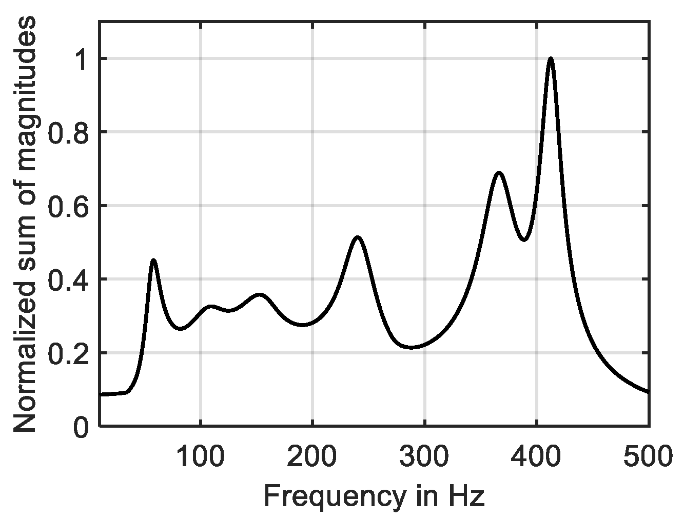
Figure 2.
Normalized mode shapes in resonance.
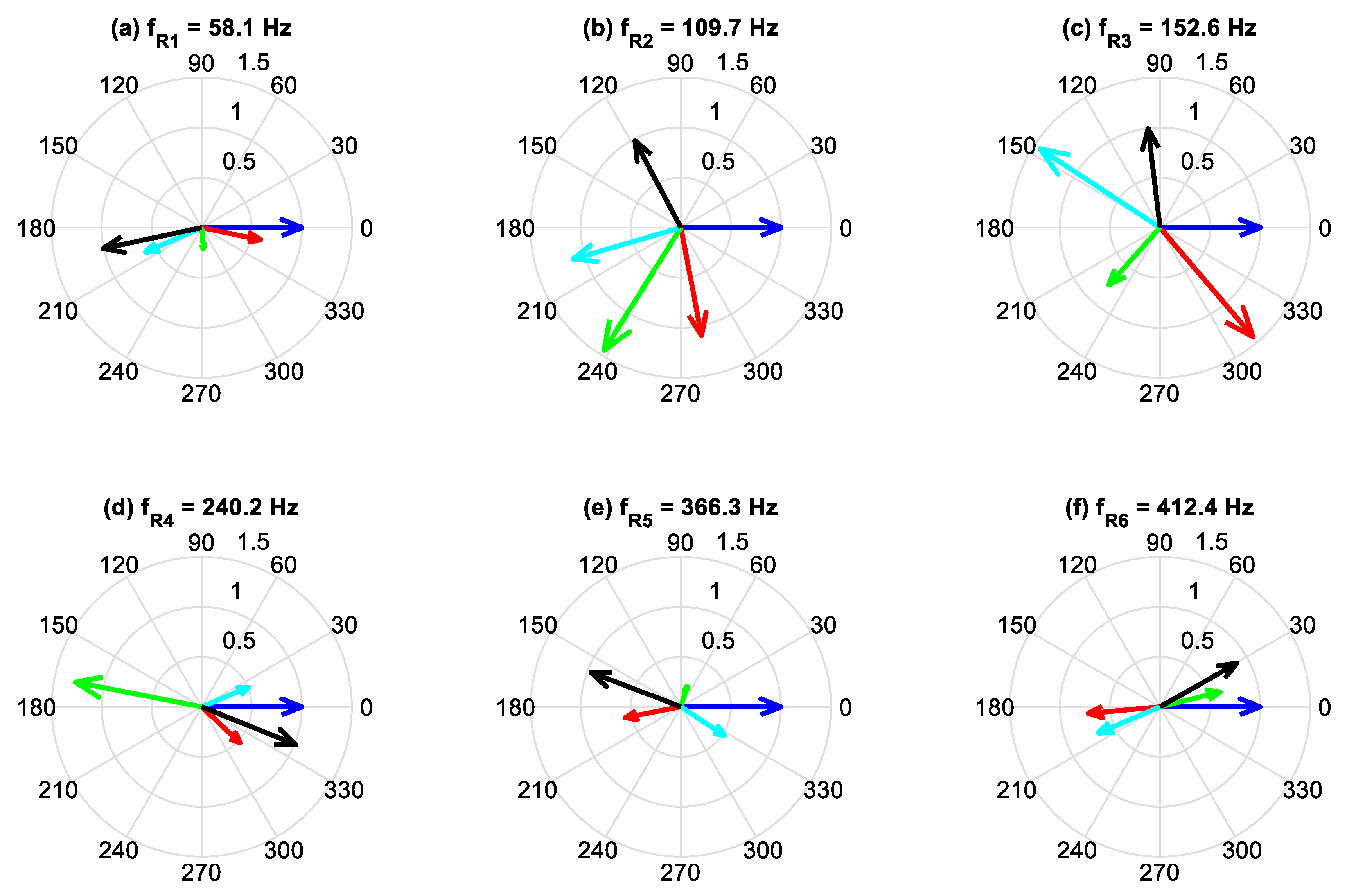
Figure 3.
System input and system output without self-adaptive control.
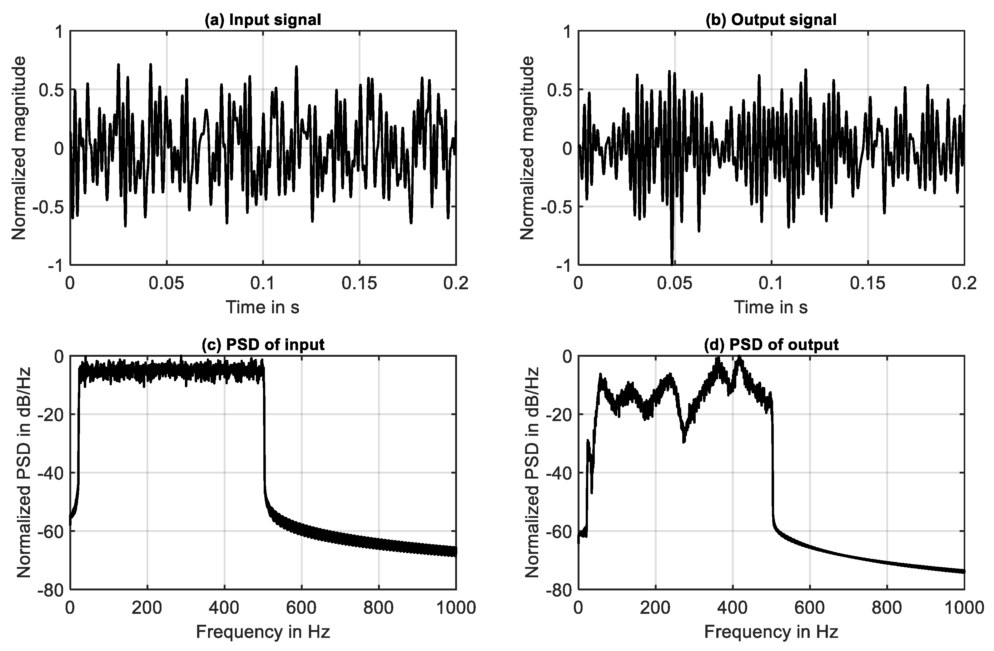
Figure 4.
IR and resonance frequencies of the uncontrolled system.
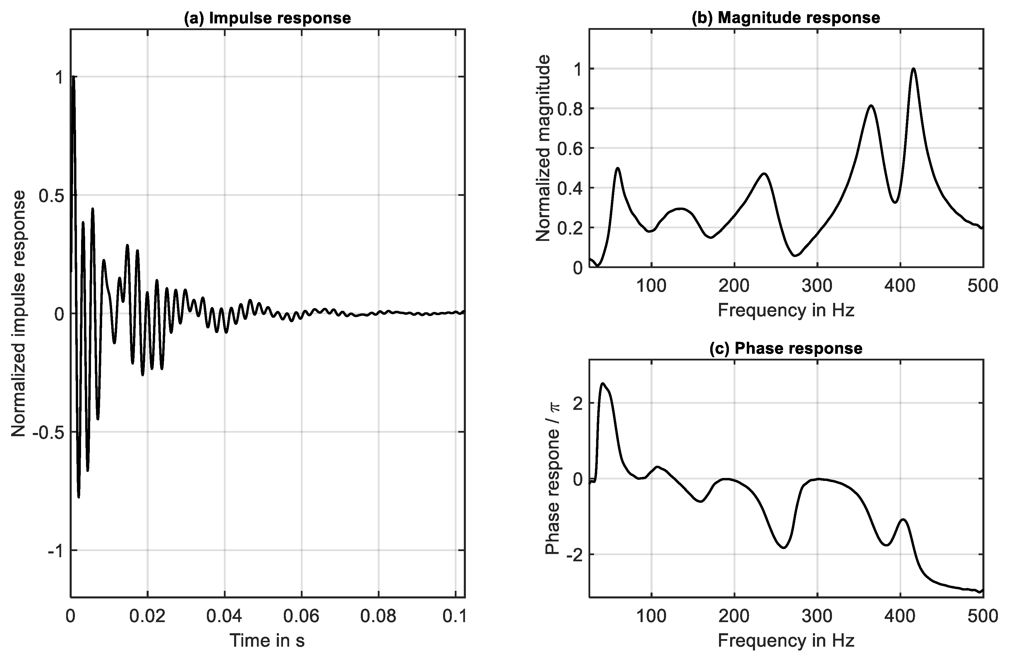
Figure 5.
Modelling of system response without active control.
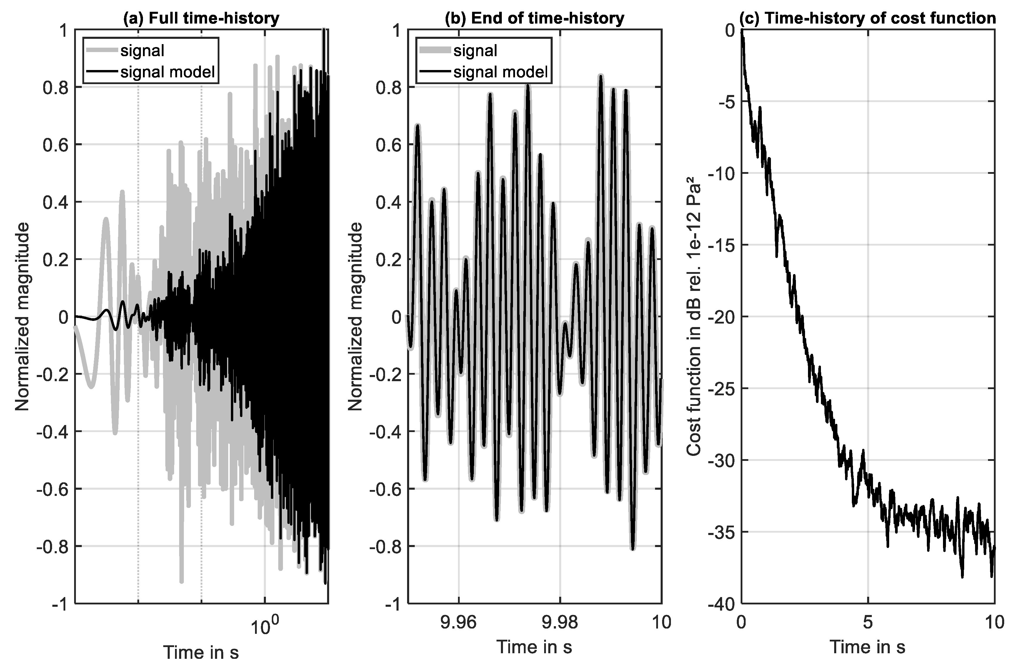
Figure 6.
Active control of local sound pressure – time-history of simulation.
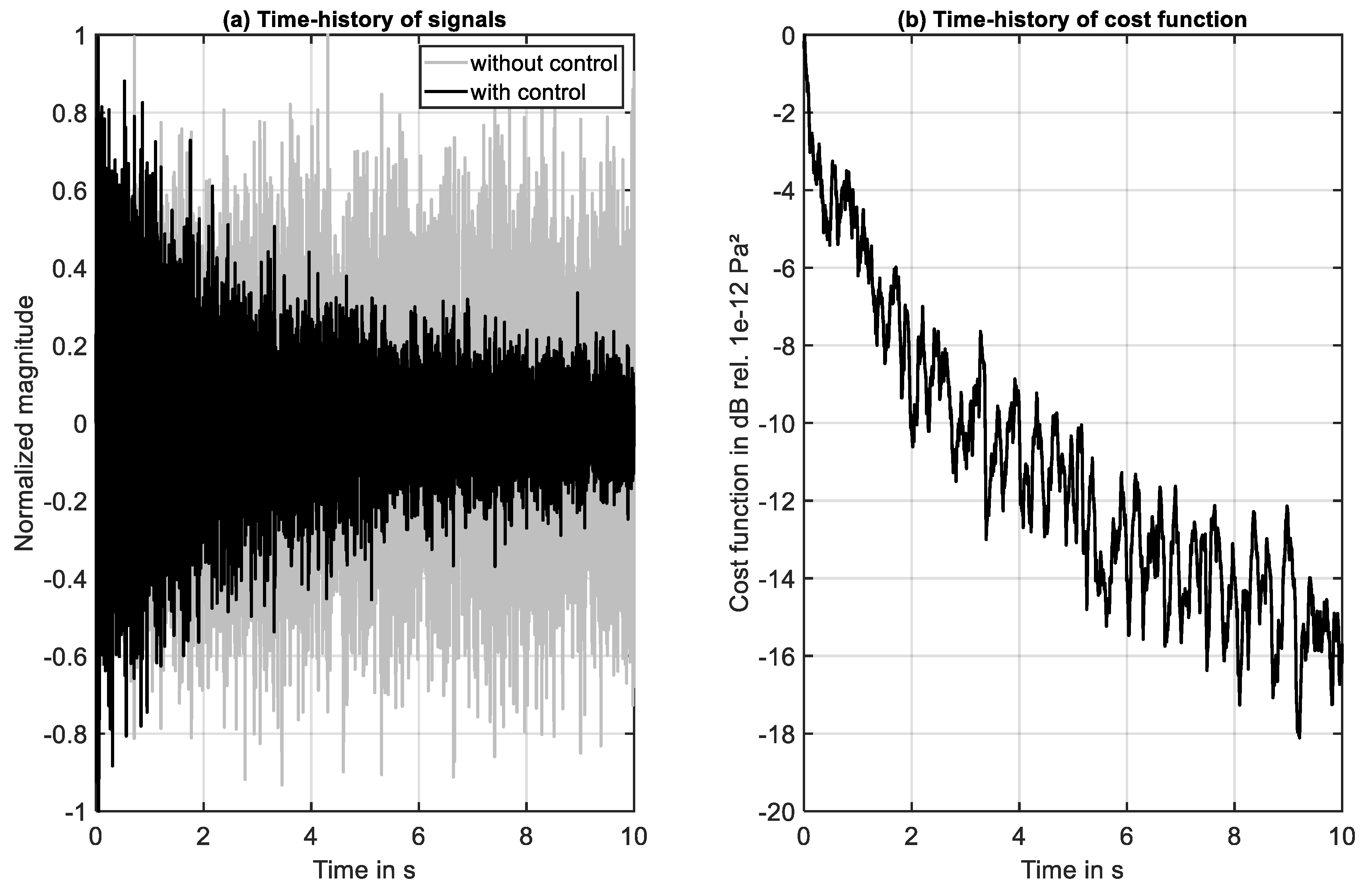
Figure 7.
Frequency domain illustration of active control of local sound pressure.
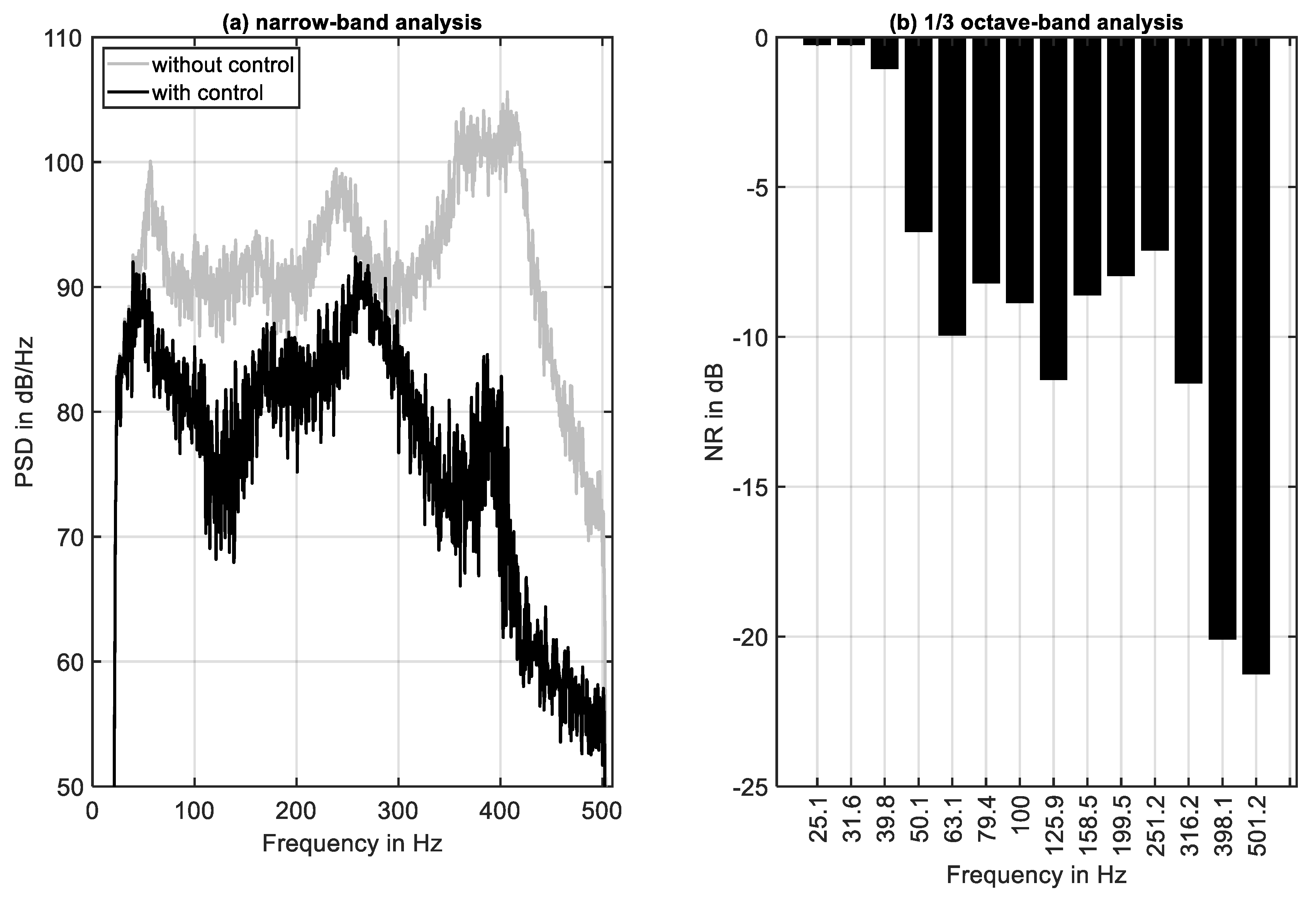
Figure 8.
Active control of local absorption – time-history of simulation.
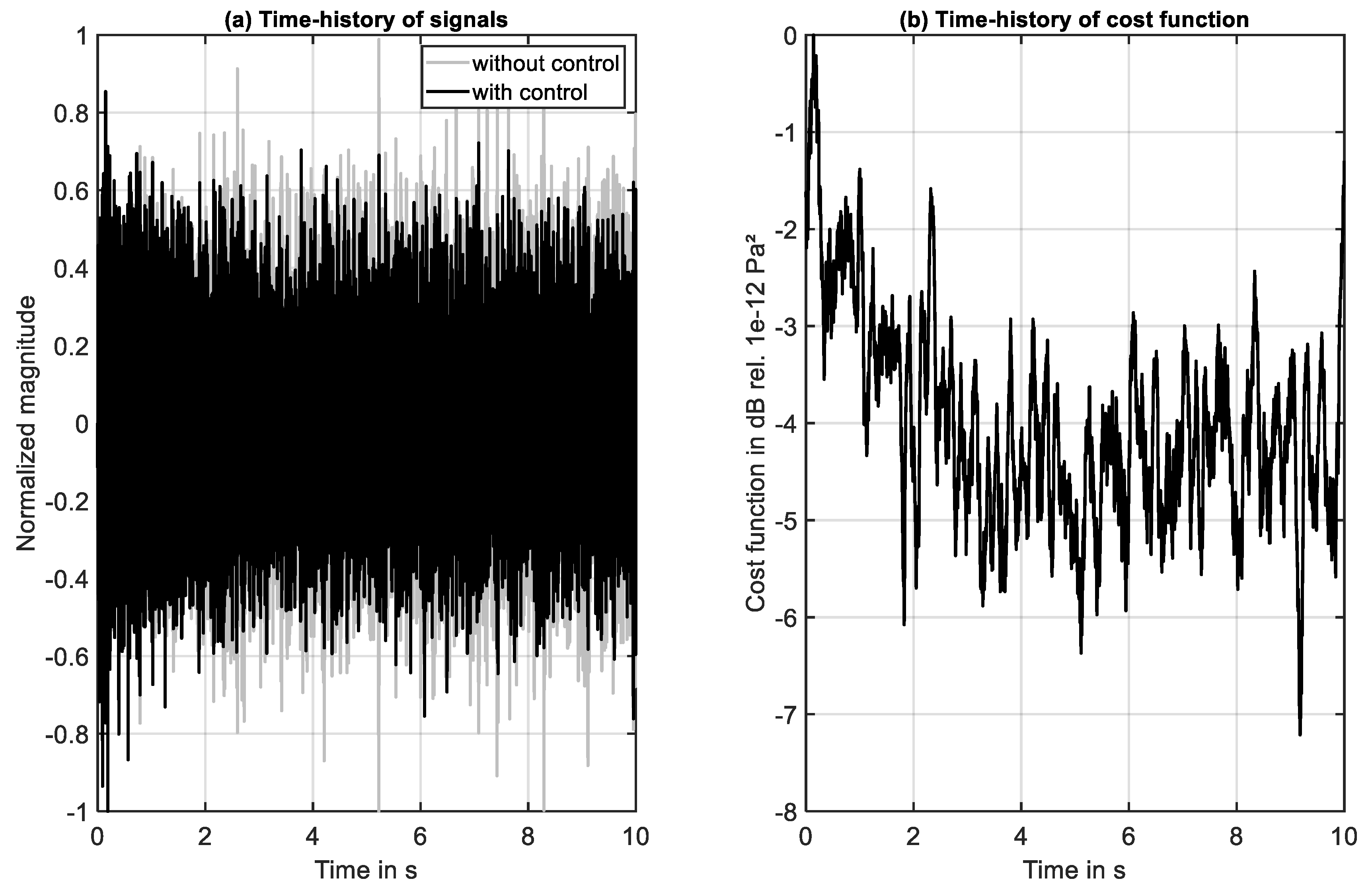
Figure 9.
Frequency domain illustration of active control of local absorption.
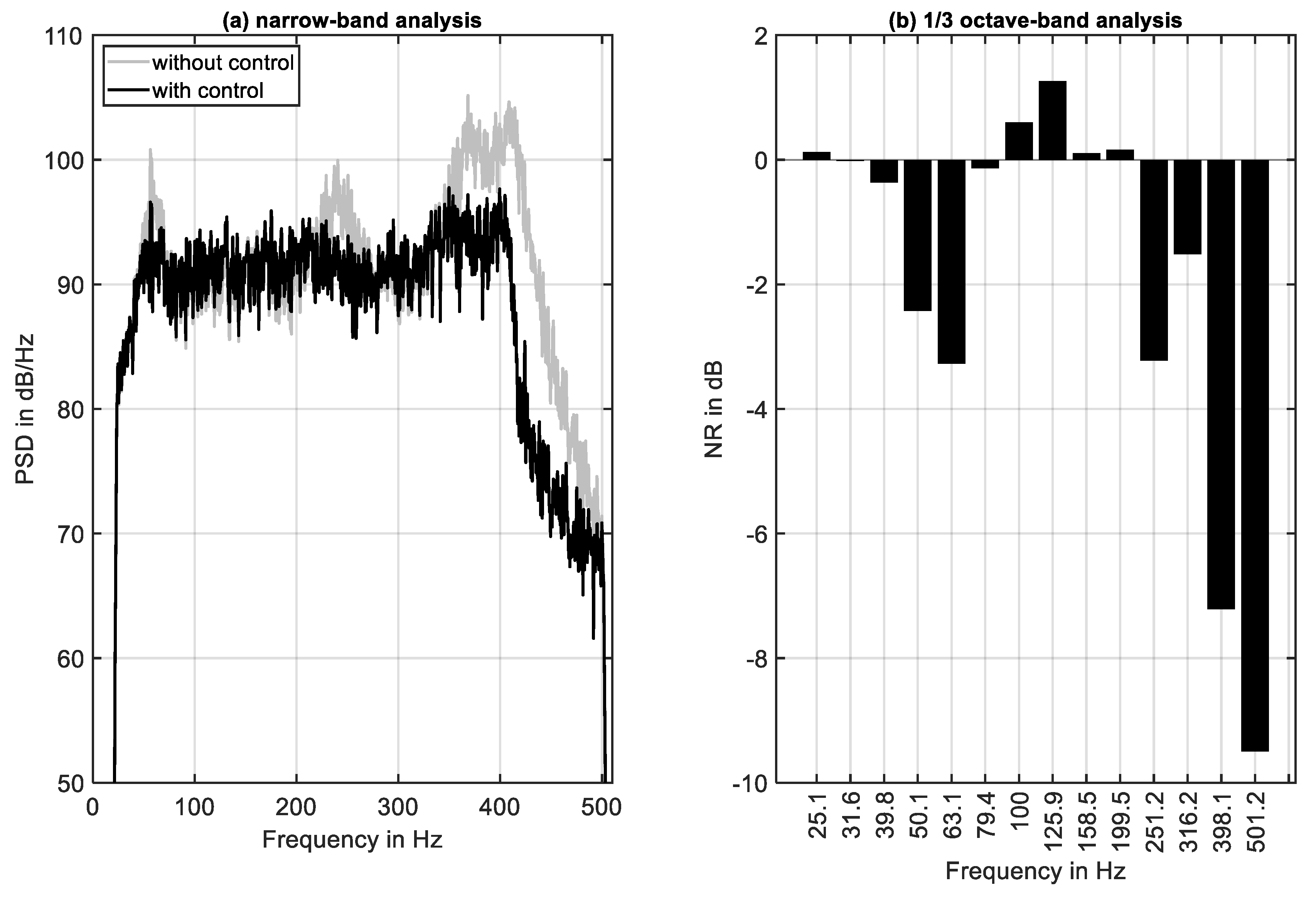

Table 1.
Parameter used for all numerical simulation.
| Parameter | Description | Value and Unit |
|---|---|---|
| Length of wave guide | 2.0 m | |
| Radius of wave guide | 0.05 m | |
| Density of air in wave guide | 1.225 kg/m3 | |
| Speed of sound in air | 343.0 m/s | |
| Viscosity of membrane | 0.43 Ns/m | |
| Stiffness of membrane | 2.45e3 N/m | |
| Mass of membrane | 4.156e-3 kg | |
| Capacitance | 0.025 F | |
| Inductance | 148.0e-6 H | |
| Resistance | 7.1 Ω | |
| Length of coil | 4.8 m | |
| Magnetic flux in coil | 0.763 T | |
| Number of time steps | 1e5 | |
| Sampling frequency | 1e4 Hz |
Table 2.
Sensor positions and color labels.
| No | Position in m | Color label |
|---|---|---|
| I | 0.0 | Blue |
| II | 0.5 | Red |
| III | 1.0 | Green |
| IV | 1.5 | Cyan |
| V | 2.0 | Black |
Table 3.
Non-zero eigenvalues, resonance frequencies, and relative error.
| No | λRe / Hz | λIm / Hz | fR / Hz | Relative deviation |
|---|---|---|---|---|
| 1 | -9.3488 | 56.776 | 58.140 | -2.3 % |
| 2 | -15.841 | 104.62 | 109.65 | -4.6 % |
| 3 | -16.115 | 156.60 | 152.55 | +2.6 % |
| 4 | -22.537 | 240.88 | 240.16 | +0.3 % |
| 5 | -19.339 | 366.05 | 366.25 | -0.1 % |
| 6 | -6.4250 | 412.69 | 412.39 | +0.1 % |
Table 4.
Normalized magnitudes at resonance frequencies.
| fR / Hz | x = 0.0 m | x = 0.5 m | x = 1.0 m | x = 1.5 m | x = 2.0 m |
|---|---|---|---|---|---|
| 58.140 | 1.00 | 0.60 | 0.21 | 0.61 | 1.00 |
| 109.65 | 1.00 | 1.10 | 1.45 | 1.12 | 0.98 |
| 152.55 | 1.00 | 1.43 | 0.77 | 1.43 | 1.00 |
| 240.16 | 1.00 | 0.53 | 1.29 | 0.51 | 1.02 |
| 366.25 | 1.00 | 0.56 | 0.22 | 0.52 | 0.96 |
| 412.39 | 1.00 | 0.72 | 0.62 | 0.67 | 0.88 |
Table 5.
Relative phase relations in grad at resonance frequencies.
| fR / Hz | x = 0.0 m | x = 0.5 m | x = 1.0 m | x = 1.5 m | x = 2.0 m |
|---|---|---|---|---|---|
| 58.140 | 0.00 | -11.78 | -85.61 | -156.5 | -168.0 |
| 109.65 | 0.00 | -79.19 | -122.0 | -163.7 | 117.8 |
| 152.55 | 0.00 | -49.61 | -131.7 | 146.7 | 96.84 |
| 240.16 | 0.00 | -43.25 | 167.0 | 22.60 | -21.91 |
| 366.25 | 0.00 | -169.0 | 73.31 | -33.36 | 159.1 |
| 412.39 | 0.00 | -174.7 | 13.87 | -156.9 | 29.61 |
Table 6.
Parameter used for plant modelling.
| Parameter | Symbol | Value |
|---|---|---|
| Non-normalized step size | 1e-2 | |
| Filter length | I | 1024 |
| Minimum signal energy | 1e-4 |
Table 7.
Parameter used for local sound pressure.
| Parameter | Symbol | Value |
|---|---|---|
| Non-normalized step size | 1e-2 | |
| Filter length | I | 1024 |
| Minimum signal energy | 1e-6 |
Table 8.
Parameter used for active control of acoustic absorption.
| Parameter | Symbol | Value |
|---|---|---|
| Non-normalized step size | 5e-3 | |
| Filter length | I | 1024 |
| Minimum signal energy | 1e-6 | |
| Time delay | 1.5e-3 s |
Disclaimer/Publisher’s Note: The statements, opinions and data contained in all publications are solely those of the individual author(s) and contributor(s) and not of MDPI and/or the editor(s). MDPI and/or the editor(s) disclaim responsibility for any injury to people or property resulting from any ideas, methods, instructions or products referred to in the content. |
© 2024 by the authors. Licensee MDPI, Basel, Switzerland. This article is an open access article distributed under the terms and conditions of the Creative Commons Attribution (CC BY) license (http://creativecommons.org/licenses/by/4.0/).
Copyright: This open access article is published under a Creative Commons CC BY 4.0 license, which permit the free download, distribution, and reuse, provided that the author and preprint are cited in any reuse.


